Variation of a Signal in Schwarzschild Spacetime
Abstract
In this paper, the variation of a signal in Schwarzschild spacetime is studied and a general equation for frequency shift parameter (FSP) is presented. It shows that FSP depends on the gravitationally-modified Doppler effects and the gravitational effects of observers. In addition, rates of time of a transmitter and a receiver may be different. When FSP is a function of the time of a receiver, FSP contributed by gravitational effect (GFSP) or gravitationally-modified Doppler effect (GMDFSP) may lead a bandlimited signal to a non-bandlimited signal. Based on the equation, FSP as a function of the time of a receiver is calculated for three scenarios: a) a spaceship moves away from a star with a constant velocity communicating with a transmitter at a fixed position; b) a spaceship moves around a star with different conic trajectories communicating with a transmitter at a fixed position; c) a signal is transmitted at a fixed position in a star system to a receiver moving with an elliptical trajectory in another star system. The studied stars are sun-like star, white dwarf and neutron star, and some numerical examples are presented to illustrate the theory.
Index Terms:
Deep space communications, general relativity, Schwarzschild spacetime, bandlimited signal, gravitationally-modified Doppler effectI Introduction
Due to the development of space technologies, human beings have sent spacecrafts to explore the space far away from Earth. After exploring the planets in the solar system, Voyager 1 of Voyager Interstellar Mission of NASA escaped the solar system and entered the interstellar medium on August 25, 2012 and is on its journey to explore the outer space [1], and Voyager 2 was at a distance of 119 AU from the sun on November 02, 2018 and is going to achieve the escape velocity to leave the solar system and explore interstellar space [2]. The success of a series of Chang’E missions inspired China to initial its first Mars Program on January 11, 2016 [3]. Focusing on deep space communications (but without considering the gravitational effect), many aspects have been discussed recently, including communication network design [3, 4, 5], channel models [6], channel coding [7], laser communications [8]. It is not hard to imagine that mankind will be able to take high-speed spaceship to explore even much deeper space in the near future. Therefore, the study of deep space communications becomes greatly important.
After Einstein field equations of general relativity were proposed [9], Schwarzschild proposed the first solution, called Schwarzschild metric[10, 11], which describes the curved spacetime around a static space object with spherical symmetry. Schwarzschild metric predicts that when an electromagnetic wave with a certain frequency at a position propagates to another position, the frequency changes as long as the gravities at the two positions are unequal. If the gravity at the latter is bigger (smaller) than that at the former, the rate of time of the latter is smaller (bigger) and the frequency blue (red) shifts. These phenomena have already been proven by a series of experiments [12, 13, 14, 15], and have been taken into account for satellite tracking [16], Global Positioning System (GPS) [17] and X-ray pulsar-based navigation by weak field approximation [18, 19, 20].
For wireless communications near the earth, Doppler effect plays an important role and communication signal frequency varies according to the relative velocity. Gravitational effect has merely been taken into account as the gravitation of Earth is not great enough to noticeably affect the spectrum of a signal. However, For wireless communications in the deep space, we will see that Doppler effect is still important (also see [21]) but should be modified, and gravitational effect becomes much more important since it may involve not only Earth but also the sun, white dwarf, neutron star or other space objects with large masses. Instead of depending on the relative velocity, the variation of frequency by gravitational effect depends on the positions of a transmitter and a receiver.
In this paper, gravitational effect on a signal is studied based on Schwarzschild metric of general relativity. The studied stars are sun-like star, white dwarf and neutron star and three different scenarios are considered: a) a spaceship moves away from a star with a constant velocity communicating with a transmitter at a fixed position; b) a spaceship moves around a star with different conic trajectories communicating with a transmitter at a fixed position; c) a signal is transmitted from a star system to another star system where the receiver is in an elliptical trajectory. The studies in this paper may help to better understand the signal models for deep space communications.
This paper is organized as follows. In Section II, a general equation for frequency shift parameter (FSP) in Schwarzshild spacetime is presented. In Section III, based on the general equation developed in Section II, the behaviors of a signal traveling in Schwarzschild spacetime are studied for the three scenarios a), b) and c) as described above. In Section IV, numerical examples for the three scenarios are presented.
: time coordinate or Newtonian time or time of a static observer at the infinity in Schwarzschild spacetime or time of a static observer in Minkowski spacetime.
: time of a static observer at in Schwarzschild spacetime.
: time of a moving observer at in Schwarzschild spacetime.
: a coordinate basis vector of partial derivative operator along direction .
a boldface English letter is a vector represented by a set of coordinate basis vectors. For example, , where is real-valued and the th component of vector (=0, time coordinate component; =1, 2, 3, space coordinate components).
: the dual vector of along direction , which is a linear operator on a vector space, i.e., , and .
: a coordinate basis tensor which is the tensor product of and and a bi-linear operator on a vector space, i.e., , and .
: Schwarzshild metric in Schwarzshild spacetime which is a bi-linear operator on a vector space and can be represented by a set of coordinate basis tensors (see (1) in the following).
: the th component of metric .
=.
=. If it is positive, is a space-like vector; if it is negative, is a time-like vector; if it is zero, is a light-like vector and vice versa. It should be noted that a time-like vector may have space coordinate components and a space-like vector may have a time coordinate component.
: is a unit space-like vector.
: is a unit time-like vector.
: Minkowski metric in Minkowski spacetime which is a bi-linear operator on a vector space and can be represented by a set of coordinate basis tensors (see (15) in the following).
II Frequency change in Schwarzschild spacetime
In Newtonian mechanics, the world is described by three dimensional space and one dimensional time with a fixed rate of time for all observers. Time and space are treated separately. A signal is a function of this time and its spectrum changes according to Doppler equation. In special relativity, the world is described by four dimensional Minkowski spacetime where a moving observer’s own time has relation with the observer’s velocity and thus time and space are mixed together. Rates of time are equal for all static observers but are different from moving observers’ rates of time. A signal is a function of its observer’s own time determined by the observer’ velocity and its spectrum changes according to the special relativity version of Doppler equation. In general relativity, the world is also described by four dimensional spacetime where time and space are mixed together as well but further take into account of gravitational effect. Rates of time may be not equal for static observers at different positions. A signal is a function of its observer’s own time determined by the observer’s velocity and position. Doppler equation should be further modified as we shall see later, and gravitational effect should be considered in calculating the change of its spectrum. Therefore, it is more complex and we will derive them next.
Schwarzschild spacetime is one solution of Einstein field equations in general relativity and describes space and time around a static object with spherical symmetry. Schwarzschild spacetime is characterized by Schwarzschild metric as follows [10, 11, 22, 23]:
| (1) | ||||
where is the gravitational constant, represents the speed of light, denotes the mass of the static object with spherical symmetry (sun, white dwarf and neutron star are regarded as static and spherically symmetric even though they may be neither static nor perfectly spherically symmetric) and are the spherical coordinates of the reference frame whose origin is the center of the object. For simplicity, we also denote and . In general, is smaller than , otherwise it is a black hole that is not discussed in this paper. Therefore, , for and for , which is the reason why the “squared length” (weighted with weights ) of a vector can be zero and even negative.
From (1), the unit vectors of four coordinates in Schwarzschild spacetime can be obtained. It should be noted that a unit time-like vector satisfies and a unit space-like vector satisfies . One unit time coordinate vector and three unit space coordinate vectors are, respectively, presented as follows:
| (2) | ||||
Note that, is not only time coordinate but also represents the time at the infinity where there is no gravitation (or Newtonian time that does not take into account of the influence of gravitation). The vector is just the unit vector of a static observer’s time direction at and the observer measures the time based on it, and is the time of the observer. The dual vector of is
| (3) |
and from the dual vector, according to [22], we can obtain:
| (4) |
where the relation between and is dependent of . It shows that if the rate of time at the infinity (or the rate of Newtonian time) is 1, the rate of time at is relatively . Therefore, rates of time are different at different , and the bigger is, the bigger rate of time is.
It is known that an electromagnetic wave is described by two parts separately: an angular frequency and a spatial wave vector . In Schwarzschild spacetime, the two parts are combined together into a four dimensional wave vector [23]:
| (5) |
where is a space-like vector and its time coordinate component is zero. In the geometrical optics approximation, is a light-like vector [23], i.e, . Z is a unit time-like vector without space coordinate component, i.e., and is a space-like vector without time coordinate component, i.e., . Thus, it is not hard to obtain:
| (6) |
When two static observers are at different positions, say , and the first observer at transmits an electromagnetic wave with angular frequency to the second observer, frequency of the received wave at obeys the following equation [23]:
| (7) |
It can be seen from (5) that angular frequency is actually the projection value after projecting along , i.e., the unit vector of a static observer’s time direction. Therefore, if the electromagnetic wave vector transmitted by a static observer at is
| (8) |
then, the electromagnetic wave vector received by a static observer at is
| (9) |
where and are unit time coordinate vector and spatial wave vector for the static observer at for , respectively. In addition, from (4) and (7), it can be seen:
| (10) |
where is the time of the static observer at for . Therefore, angular frequency is inversely proportional to rate of time if two observers are static. Obviously, if , the frequency red shifts and if , the frequency blue shifts.
Now, consider that a new observer at is not static but with four dimensional velocity (also called 4-velocity [23]):
| (11) | ||||
where
| (12) | ||||
is the spatial velocity of the new observer in Schwarzschild spacetime and is a space-like vector without time coordinate component. The second equality in (12) is according to (4) with and . Let , which is the magnitude of the spatial velocity at in Schwarzschild spacetime [23]. Then,
| (13) | ||||
where the term in the first equality is from .
It should be noted that is the unit vector of the new observer’s time direction. The new observer measures the time based on and is the time of the new observer. To be more explicit, two examples are illustrated in Fig. 1. The coordinates in Fig. 1 are combinations of three dimensional space and one dimensional time into four dimensional spacetime (only two dimensions are depicted for simplicity). A curve in the coordinates is time vs. space and called an observer’s world line which is parametrized by or characterized by tangent vector . A time-like curve means that every tangent vector of the curve is a unit time-like vector [22]. Since every observer should not be faster than light, every world line of an observer is a time-like curve, is precisely the time of the observer along the curve and is like a ruler for the observer to measure the time. In sub-figure (a), an observer at is static, the tangent vector of every position on the curve is , and thus the observer’s time is . In sub-figure (b), an observer is moving with different velocities at different positions and its tangent vector is changing all the time, but at every position of its world line, it measures the time along the curve using the tangent vector as a ruler. Since the 4-velocity is a unit time-like vector, i.e., , is a unit time-like vector without space coordinate component, and is a space-like vector without time coordinate component, we have and . Then, it is not hard to obtain:
| (14) |
For the comparison purpose, in special relativity, the four dimensional spacetime is Minkowski spacetime. The metric characterizing the Minkowski spacetime is Minkowski metric (also called flat metric) [23]:
| (15) |
and let be the spatial velocity in Minkowski spacetime. Then,
| (16) |
and the magnitude of the spatial velocity in Minkowski spacetime can be calculated:
| (17) | ||||
It can be seen from (12) and (16) that one difference of the spatial velocities in the two spacetimes is that Newtonian time (a static observer’s time at in Minkowski spacetime) in (16) is just replaced by time (a static observer’s time at in Schwarzschild spacetime) in (12), though they share the same direction. Another difference is in the magnitudes of the spatial velocities in the two spacetimes. By comparing (13) and (17), there is one more coefficient in the first equality of (13) which is derived from in , in addition to the time difference of and .
According to (14), and (4) with and , we have
| (18) |
Since the frequency at for the new observer is the component of its own time direction, it is needed to project along , i.e., the unit vector of the new observer’s time direction, and the projection value is
| (19) | ||||
where is the frequency for a static observer at who shares the same with the moving observer at but has different time direction, and . The second equality in (19) is according to (9), (11) and (14), the second last equality is according to with , and the last equality is according to . We denote
| (20) |
and is called frequency shift parameter (FSP) and is independent of angular frequency . Thus, the frequency at of the moving observer in terms of the signal frequency of the transmitter is
| (21) |
It is not hard to see that FSP in (20) can be separated into two parts. The first part is
| (22) |
which is similar to the special relativity version of the Doppler equation [23],
| (23) |
where is similar to in (14) but with replaced by , and is the intersection angle between and . When , (22) and (23) are equivalent. Furthermore, if , then and we have
| (24) |
which is the conventional version of the Doppler equation. Therefore, (22) is just a gravitationally-modified Doppler equation and is called gravitationally-modified Doppler frequency shift parameter (GMDFSP).
The second part is purely derived from gravitational effect (or called Einstein effect in [24]), and is called gravitational frequency shift parameter (GFSP):
| (25) |
Thus, FSP can be rewritten as
| (26) |
It is clear that when is much different from 1, and in (21) are much different, i.e., the signal frequency of a moving observer at and the signal frequency of a transmitter at are much different. This means that there is a large frequency shift. Since is comprised of and , the contributions from the two parts can be considered separately. If the difference of and 1 (or and 1) is large or small, gravitationally-modified Doppler effect (or gravitational effect) is significant or negligible.
When an observer at is static, (19) comes back to (7), since and , and the FSP in (20) is equal to and is constant. Also, when or in (22) changes over the time , is a function of time , and when or in (25) changes over the time , is also a function of time . As a result, in (20) and the frequency in (21) are functions of time . In addition, since , and since and , in general. Therefore, .
III A signal in Schwarzschild spacetime
After the basic principle has been established above for the FSP when an electromagnetic wave is propagating through Schwarzschild spacetime, the variation for a signal transmitted in Schwarzschild spacetime in a particular scenario is not hard to see. In this section, to be consistent with Section II, we denote the time of a transmitter at a fixed position , the time of a moving receiver at and the time at infinity as , and , respectively. Without considering noise, when a single-frequency complex exponential signal is transmitted at to a spaceship at , the received signal by the spaceship will be different, that is:
| (27) |
where , and is the FSP in (20). If is constant, . A periodical signal with fundamental angular frequency can be expanded as Fourier series:
| (28) |
and
| (29) |
Then, the received signal is
| (30) |
For a non-periodic signal, its fundamental angular frequency can be regarded as infinitesimal . Then, the transmitted signal can be expanded as [25]:
| (31) |
and
| (32) |
Then, the recieved signal is
| (33) | ||||
As , the received signal can be rewritten as
| (34) | ||||
where is the Fourier transform of .
In general, a communication signal is bandlimited and a bandlimited signal of bandwidth is
| (35) |
If is a non-zero constant, according to (34), the received signal is
| (36) |
Then, the spectrum of the received signal is broadened when , narrowed when and kept unchanged when . If is a function of time , the received signal is . Inferred from [26], if is not constant, is a non-bandlimited signal. Thus, a bandlimited signal becomes non-bandlimited when it is transmitted through Schwarzschild spacetime. Clearly, the higher the varying rate of is, the higher the non-bandlimited-ness is. The contribution to the non-bandlimited-ness consists of gravitationally-modified Doppler effect and gravitational effect. If the varying rate of (or ) is large, the non-bandlimited-ness contributed by (or ) is significant; if it is small, the non-bandlimited-ness contributed by (or ) may be negligible.
III-A Variation of a signal for straight trajectory
In this section, we consider one of the simplest cases that a receiver is moving away from a star with being constant, and a transmitter’s position , the receiver’s position and the center of the star are at the same line as shown in Fig. 2. Suppose when the receiver’s time , as a function of is zero and the receiver begins to receive a signal from the transmitter at position . At Newtonian time when the receiver’s time is ,
| (37) |
| (38) | ||||
Newtonian time as a function of can be obtained from (18), (37) and (38):
| (39) | ||||
where the relation between and depends on and , and as long as and are provided, as a function of is fixed. in (19) . Therefore, from (22), (25), (37), (38) and (39), GMDFSP and GFSP are, respectively,
| (40) | ||||
Since just depends on the coefficients and , the coefficients that FSP depends on are also and .

No speed is bigger than the speed of light, i.e., . If , then
| (41) | ||||
where is not far away from 1 in general, and can be written as
| (42) |
and
| (43) |
Since the studied stars are not black hole, , as mentioned in Section II. If , i.e., the star is far away from being a black hole, then from (42),
| (44) | ||||
and from (43),
| (45) |
Since ,
| (46) |
Furthermore, if , i.e., the flying distance of the spaceship during the time of communications is relatively short, then from (44),
| (47) | ||||
where
| (48) | ||||
and from (46),
| (49) |
where . Consequently, after a signal is transmitted at to the spaceship at , the received signal by the spaceship is
| (50) |
where . It can be seen from [26] that if is bandlimited, then is not bandlimited anymore. Is bandlimited in fractional Fourier domain [27, 28]? To answer this question, firstly consider a single-frequency signal
the received signal by the spaceship is
which is a chirp signal with initial frequncy and frequency rate . Therefore, is bandlimited in the fractional Fourier domain with frequency rate . However, if is not single-frequency, then is non-bandlimited in any fractional Fourier domain. To see this, let us consider the following signal of two single frequencies:
with . Then, the received signal by the spaceship is
Notably, and are both chirp signals but with different frequency rates; therefore it is impossible to find a common fractional domain where both fractional Fourier transforms of and are bandlimited [29]. As a consequence, is not bandlimited in fractional Fourier domain. This applies to any non-single-frequency signal.
III-B Variation of a signal for conic trajectories
In general, when moving around a star with no extra force, a spaceship may follow a conic trajectory. Therefore, it is worthwhile calculating the change of a signal when the spaceship follows such a trajectory. There are three different kinds of trajectories: ellipse, parabola and hyperbola as shown in Fig. 3. Whether it is elliptical, parabolic or hyperbolic depends on the mechanical energy of the spaceship which is equal to the sum of gravitational potential energy () and kinetic energy (). If the mechanical energy is smaller than 0, then the trajectory is elliptical. If the mechanical energy is equal to 0, then the trajectory is parabolic. If the mechanical energy is bigger than 0, then the trajectory is hyperbolic.
Consider the transmitter’s position is just a fixed position close to a star and a spaceship with the receiver aboard is moving around the star with a conic trajectory, and its radius relative to the center of the star is [30]
| (51) |
and
| (52) |
where and is the eccentricity of the trajectory (ellipse, ; parabola, ; hyperbola, ), and is the mass of the spaceship. The mechanical energy and the angular momentum are constants based on mechanical energy conservation and angular momentum conservation, respectively, is Newtonian time, and where is the mass of the star. If the semi-major axis of its orbit is known, then
| (53) |
Combining (51) and (52), the angular velocity in Newtonian time is
| (54) |
The radial velocity of the spaceship relative to the center of the star in Newtonian time is
| (55) |
Since , according to (12), (13), (51), (54) and (55),
| (56) |
and,
| (57) |
Then, according to (18), (51), (54) and (57),
| (58) | ||||
Suppose the transmitted signal approximately propagates along straight lines. Then, since , in (9), let
| (59) |
where is a parameter and is the intersection angle between and the radial direction at . From Fig. 3 (b), it is not hard to see,
| (60) | ||||
According to (6) with and , (59) and (60),
| (61) |
Then, according to (56), (59), (60) and (61), in (19) is
| (62) |
where
| (63) | ||||
As long as the initial value of and the values of and (or and ) are given, as a function of can be obtained from (51) and (58). Next, it can be seen from (51), (57) and (62) that , and are functions of ; therefore, they are also functions of . Neglecting the hindrance by the star on signals, if the spaceship does not use any extra force, according to (20), FSP as a function of is
| (64) |
and
| (65) | ||||
are the GMDFSP and GFSP, respectively.

III-C Variation of a signal for interstellar communications
Mankind may have chances to receive signals from aliens in another faraway star system who may find it not so hard to send an electromagnetic wave containing information to solar system. Besides, mankind may be able to settle on many other star systems in the future, so communications between different star systems may be frequent. Therefore, It is worth calculating the change of a signal between different star systems.
Consider a signal is transmitted from a star system A to another faraway star system B and the relative velocity between the two stars is fixed with a magnitude in Newtonian time along a fixed direction as shown in Fig. 4. Since the two stars are far away from each other, the gravitation of one star can be neglected if the signal is much closer to the other star. When the signal is near the transmitter, the gravitational effect is almost caused by star A. When the signal is near the receiver, the gravitational effect is almost caused by star B. However, when the signal is neither near star A nor star B, the gravitation can be neglected. Therefore, the whole process can be separated into two parts: a) the signal is propagating from the transmitter’s position near star A to a position which is far away from star A and star B (called the faraway position in the following) and is moving with the same velocity as star B; b) the signal is propagating from the faraway position to the receiver’s position near star B. In the process a), it is the same as that considered in Section III-A as shown in Fig.2. Set the parameter of the frequency shift as . Since the faraway position and the faraway position is moving away from transmitter position with velocity , according to (20), if the position of transmitter is fixed, then
| (66) |
where , is the mass of star A, is the radial distance of the transmitter relative to the center of star A.
In the process b), it is similar to that in Section III-B as shown in Fig. 3 (a). Set the parameter of the frequency shift as . Suppose the receiver at position follows an elliptical trajectory, according to (51)
| (67) |
where . Let be the spatial velocity of the receiver in Schwarzschild spacetime, according to (57),
| (68) |
Substituting in (62) for ,
| (69) | ||||
and according to (58),
| (70) | ||||
where is the time of the receiver and as a function of can be solved. It can be seen from (67), (68) and (69) that , and are functions of , i.e., functions of . Therefore, according to (20), as a function of is
| (71) |
Combining processes a) and b), the FSP of the whole process is
| (72) | ||||
and
| (73) | ||||
are the GMDFSP and GFSP, respectively.
III-D Variation of a signal transmitted from a moving position to a moving spaceship
In the above studies, a transmitter is at a fixed position. The above results can be easily extended to the case when the transmitter is in motion as follows.
A moving transmitter has its own 4-velocity and its frequency is just the projection value along its 4-velocity. Suppose the frequency of a signal that the moving transmitter at transmits is . Then, the relation between the frequencies of a static observer at and the moving transmitter at can be obtained by using (19) with replaced by :
| (74) |
where , is the spatial wave vector at , and is the spatial velocity of the moving transmitter in Schwarzschild spacetime and is the magnitude. Then, by using (19) again without modification, i.e., the relation between the frequencies of a moving observer at and a static observer at , the frequency of a moving receiver at is
| (75) |
where , is the spatial wave vector at , and is the spatial velocity of the moving receiver in Shwarzschild spacetime and is the magnitude. Then,
| (76) |
IV Numerical examples
In this section, we present some numerical examples to illustrate what we have studied above. The studied stars are sun-like star, white dwarf and neutron star. The mass of the sun is approximately and its radius is about [31]. The mass of the white dwarf is set as and its radius as which is nearly the radius of the earth. The mass of the neutron star is set as and its radius as or . All these settings are according to [32, 33, 34, 35, 36, 37, 38, 39].
IV-A Spaceship moving away from a star
In this section, consider transmitting a signal at a fixed position to a spaceship moving away from the sun, a white dwarf or a neutron star as shown in Fig. 2. In all examples is set as the third cosmic velocity .
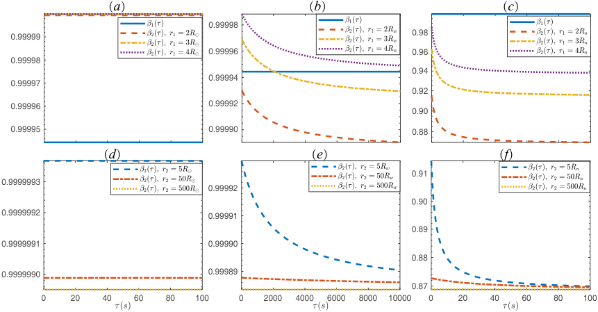
In Figs. 5 , , , the initial distances of the receiver to the centers of the sun, the white dwarf and the neutron star, when it begins to receive signals, are , and , respectively. Compared to gravitationally-modified Doppler effect , gravitational effect is negligible in the solar system since GFSP is much close to 1 in all three cases. As and are both nearly constant, the non-bandlimited-ness due to gravitationally-modified Doppler effect and gravitational effect is negligible in the solar system. In contrast, when the transmitter and the receiver are both not far from the white dwarf, gravitational effect is comparable to gravitationally-modified Doppler effect and the non-bandlimited-ness contributed by gravitational effect is noticeable. When the transmitter is close to the neutron star, compared to the gravitational effect, gravitationally-modified Doppler effect can be neglected, and the frequency rate contributed by is huge, which causes a high non-bandlimited-ness. In Figs. 5 , , , whether the communications is in the solar system, the white dwarf system or the neutron star system, when the receiver is faraway, is nearly constant (see the curves of , , ). This is because when the receiver is far away from them, the gravitation on the receiver becomes negligible. As a result, the frequency rate is very small and the non-bandlimited-ness is less noticeable.
Fig. 6 is to show the difference of gravitationally-modified Doppler effect and Doppler effect (special relativity version) , and the difference of the time of a moving receiver and Newtonian time . Since the gravitation in neutron star system is much higher than that in other star systems, these differences are much clearer in a neutron star system. Therefore, a neutron star system is chosen to show these differences. In Fig. 6 , it shows that gravitationally-modified Doppler effect is more than Doppler effect since is closer to 1, but the difference gradually tends to be zero as the receiver is far away from the neutron star. Although the Fig. 6 shows that is approximately linear to , the difference between and in Fig. 6 increases drastically in the beginning and then tends to be linear to .
In Fig. 7, to show the non-bandlimited-ness of a signal in these star systems, the FFTs of a special bandlimited signal—a single-frequency complex exponential signal transmitted in the solar system, the white dwarf system or the neutron star system during different time periods are calculated. In the solar system, the FFTs with and without gravitational effect are nearly the same during the same time periods. The bands with and without gravitational effect are both very narrow centering around centric frequency Hz. In the white dwarf system, the FFTs are close to each other, but the FFT with gravitational effect has a relative translation to the left. The bands with and without gravitational effect are both very narrow while centering around a little different frequencies. In the neutron star system, when the period of time is small, the FFT with gravitational effect spans over a broad frequency band and peaks at much smaller frequency, compared with the band without gravitational effect. However, when the period of time is large, the band with gravitational effect is narrowed.
IV-B Spaceship moving around a star with conic trajectories
In this section, we consider transmitting a signal at a fixed position to a spaceship moving around the sun, a white dwarf or a neutron star with elliptical, parabolic or hyperbolic trajectory as shown in Fig. 3.
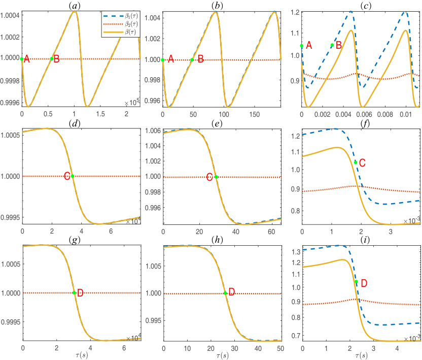
In Figs. 8 , compared to gravitationally-modified Doppler effect in all three cases, gravitational effect and the non-bandlimited-ness contributed by gravitational effect are both negligible in the solar system. In Figs. 8 , , , though small, the differences of and can be noticed in all trajectories around the white dwarf. Therefore, gravitational effect should be taken into account in the white dwarf system. However, the non-bandlimited-ness contributed by gravitational effect is negligible in all trajectories because of little variation of . In Figs. 8 , , , when the spaceship moves around the neutron star, the gravitational effect is significant. The variation of is noticeable, especially in the elliptical trajectory, and the non-bandlimited-ness contributed by gravitational effect cannot be ignored. However, the variation of is more significant. Therefore, the non-bandlimited-ness contributed by gravitationally-modified Doppler effect is more significant.
Whether the star is the sun, the white dwarf or the neutron star, the non-bandlimited-ness is mainly contributed by gravitationally-modified Doppler effect. Furthermore, in the elliptical trajectories, when the spaceship is around the position that is closest or farthest to the transmitter (see position A and position B in Fig. 3 and Fig. 8), the frequency rate derived from is high, which leads to a high non-bandlimited-ness. For parabolic and hyperbolic trajectories, when the spaceship is around the closest position to the transmitter (see position C and position D in Fig. 3 and Fig. 8), the frequency rates are also high while they are nearly zero when the spaceship is far away from the transmitter. The levels of non-bandlimited-ness in the solar system, the white dwarf system and the neutron star system are different. Obviously, the level of non-bandlimited-ness is the highest in the neutron star system, followed by the white dwarf system. In the solar system, the non-bandlimited-ness can be neglected.
Since gravitational effect in the solar system or the white dwarf system is not significant and the variation of is more significant in the elliptical trajectory, only the spectrum of a signal transmitted to a spaceship following an elliptical trajectory in the neutron star system is analyzed. In Fig. 9, when only taking gravitational effect into account, the single-frequency complex exponential signal expands over a noticeable frequency band. This confirms that gravitational effect has a contribution to the non-bandlimited-ness. When only taking gravitationally-modified Doppler effect into account, the signal expands over even more wider frequency band. The whole effect has the similar effect as gravitationally-modified Doppler effect, which confirms that the non-bandlimited-ness is mainly determined by gravitationally-modified Doppler effect.
IV-C Communications between different star systems
In this section, gravitational effect on a signal is calculated when it is transmitted from a sun-like star, a white dwarf or a neutron star system to another sun-like star, white dwarf or neutron star system as shown in Fig. 4. The receiver moves with an elliptical trajectory. The mass and the radius of the sun-like stars are the same as the sun. Suppose the communications lasts from a few seconds to a few minutes. in (72) is set as .
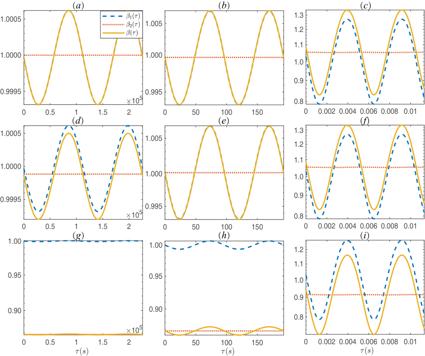
In Figs. 10 , , , a signal sent by intelligent species in another system comes to the solar system during a relatively short period of time. If the signal comes from a sun-like system, gravitational effect can be neglected. If the signal comes from the white dwarf system, gravitational effect is comparable to gravitationally-modified Doppler effect. If the signal comes from the neutron star system, gravitational effect is significant and gravitationally-modified Doppler shift is relatively small. However, whatever the signal source system is, the FSP is nearly constant during a relative small period of time. As a result, the frequency rate is nearly zero and the non-bandlimited-ness is negligible.
In Figs. 10 , , , a signal from a star system is transmitted to a white dwarf system. On one hand, if the source star system is a sun-like star system or a white dwarf system, gravitational effect can be simply neglected. On the other hand, if the source star is a neutron star, gravitational effect is significant, compared to gravitationally-modified Doppler effect. However, is nearly constant and the non-bandlimited-ness contributed by gravitationally-modified Doppler effect is dominant. Therefore, neither gravitational effect nor gravitationally-modified Doppler effect can be ignore, and gravitational effect provides large frequency shift and gravitationally-modified Doppler effect provides high non-bandlimited-ness. In any case, the frequency rate is noticeable and the non-bandlimited-ness is significant.
In Figs. 10 , , , a neutron star receives a signal from a star system. On one hand, for all three cases, gravitationally-modified Doppler effect and the non-bandlimited-ness contributed by gravitationally-modified Doppler effect are both significant. On the other hand, for all the three cases, the differences of and 1 are all large and gravitational effect is significant, but is nearly constant, compared to . Therefore, the non-bandlimited-ness is mainly contributed by gravitationally-modified Doppler effect.
V Conclusion
In this paper, the variation of a signal in Schwarzschild spacetime was studied and a general equation for frequency shift parameter (FSP), which can be divided into gravitational FSP and gravitationally-modified Doppler FSP, was presented. In addition, rates of time of a transmitter and a receiver may be different. Based on the equation for FSP, FSP as a function of the time of a receiver was calculated for scenarios a), b), and c) as described in Abstract. In scenario a), compared to gravitationally-modified Doppler effect, gravitational effect is negligible in the solar system, comparable in a white dwarf system, and more significant in a neutron star system, which suggests that for deep space missions in the solar system like Mars exploration, gravitational effect can be neglected. The non-bandlimited-ness is only contributed by gravitational effect and is more significant in a neutron star system. Furthermore, choosing a neutron star as an example, when a receiver is close to the neutron star, the difference between gravitationally-modified Doppler effect and the special relativity version of Doppler effect, and the difference between time of a moving receiver and Newtonian time are both significant. In scenario b), gravitational effect, similar to scenario a), is insignificant in the solar system, less significant in a white dwarf system and significant in a neutron star system. The non-bandlimited-ness is mainly contributed by gravitationally-modified Doppler effect in all star systems, but the non-bandlimited-ness in the neutron star system cannot be neglected. In scenario c), when communications is between a sun-like star system and another sun-like star system (or a white dwarf system and another white dwarf system), gravitational effect is negligible; when it is between a white dwarf and a sun-like star, gravitational effect is insignificant if a receiver is in a white dwarf system while significant if a receiver is in a sun-like star system; when it involves a neutron star, gravitational effect cannot be ignored and is comparable to gravitationally-modified Doppler effect. In all the cases of scenario c), the non-bandlimited-ness is mainly contributed by gravitationally-modified Doppler effect.
Although in the most of this paper, the position of a transmitter was fixed, as mentioned and studied in Section III-D, all the results can be easily extended to the case when a transmitter moves. Finally, the studies in this paper may help to better understand the signal models in deep space communications.
References
- [1] Barnes B. In a breathtaking first, NASA craft exits the solar system. New York Times, Sept 12, 2013.
- [2] Gill V. NASA’s Voyager 2 probe ‘leaves the solar system’. BBC News, Dec 10, 2018.
- [3] Zhao K, Zhang Q. Network protocol architectures for future deep-space internetworking. Sci China Inf Sci, 2018, 64(4): 040303.
- [4] Wu W, Tang Y, Zhang L, et al. Design of communication relay mission for supporting lunar-farside soft landing. Sci China Inf Sci, 2018, 64(4): 040305.
- [5] Wan P, Zhan Y, Pan X. Solar system interplanetary communication networks: architectures, technologies and developments. Sci China Inf Sci, 2018, 61(4): 040302.
- [6] Pan X, Zhan X, Wan P, et al. Review of channel models for deep space communications. Sci China Inf Sci, 2018, 61(4): 040304.
- [7] Wu S, Li S, Wang Z, et al. Novel distributed UEP rateless coding scheme for data transmission in deep space networks. Sci China Inf Sci, 2018, 61(4): 040306.
- [8] Wu W, Chen M, Zhang Z, et al. Overview of deep space laser communication. Sci China Inf Sci, 2018, 61(4)” 040301.
- [9] Einstein S. Die feldgleichungen der gravitation. Sitzungsberichte der Preussischen Akademie der Wissenschaften zu Berlin, 1915, 844–847.
- [10] Schwarzschild K. Über das gravitationsfeld eines massenpunktes nach der einsteinschen theorie. Sitzungsberichte der Deutschen Akademie der Wissenschaften zu Berlin, Klasse fur Mathematik, Physik, und Technik, 1916, 189.
- [11] Schwarzschild K. Über das gravitationsfeld einer kugel aus inkompressibler flussigkeit nach der einsteinschen theorie. Sitzungsberichte der Deutschen Akademie der Wissenschaften zu Berlin, Klasse fur Mathematik, Physik, und Technik, 1916, 424.
- [12] Pound R V, Rebka Jr G A. Gravitational red-shift in nuclear resonance. Phys Rev Lett, 1959, 3(9): 439–441.
- [13] Pound R V, Snider J L. Effect of gravity on gamma radiation. Phys Rev, 1965, 140(3B): 788-803.
- [14] Snider J L. New measurement of the solar gravitational red shift. Phys Rev Lett, 2001, 28(13): 853–856.
- [15] Turner K C, Hill H A. New experimental limit on velocity-dependent interactions of clocks and distant matter. Phys Rev, 1964, 134(1B): 252–256.
- [16] Harkins M D. The relativistic Doppler shift in satellite tracking. Radio Sci, 1979, 14(4): 671–675.
- [17] Love A W. GPS, atomic clocks and relativity. IEEE Potentials, 2002, 13(2): 11–15.
- [18] Hanson J E. Principles of X-ray navigation. Dissertation for the Doctoral Degree. Palo Alto: Stanford University, 1996.
- [19] Sheikh S I. The use of variable celestial X-ray sources for spacecraft navigation. Dissertation for the Doctoral Degree. College Park: University of Maryland, 2005.
- [20] Sheikh S I, Pines D J, Ray P S, et al. Spacecraft navigation using X-ray pulsars. J Guid. Control Dynam, 2006, 29(1): 49–63.
- [21] Oberg J. Titan calling. IEEE Spectrum, 2004, 41(10): 28–33.
- [22] Misner C W, Thorne K S, Wheeler J A. Gravitation. San Francisco: W H Freeman and Company, 1973.
- [23] Wald R M. General Relativity. Chicago: The University of Chicago Press, 1984.
- [24] Møller C. The Theory of Relativity, 2nd ed. Oxford: Clarendon Press, 1972.
- [25] Oppenheim A V, Willsky A S, Nawab S H. Signals and Systems, 2nd ed. New Jersey: Prentice-Hall, 1996.
- [26] Xia X-G, Zhang Z. On a conjecture on time-warped band-limited signals. IEEE Trans Signal Process, 1992, 40(1): 252–254.
- [27] Almeida L B. The fractional Fourier transform and time-frequency representations. IEEE Trans Signal Process, 1994, 42(11): 3084–3091.
- [28] Tao R, Li B Z, Wang Y. Spectral analysis and reconstruction for periodic nonuniformly sampled signals in fractional Fourier domain. IEEE Trans Signal Process, 2007, 55(7): 3541–3547.
- [29] Xia X-G. On bandlimited signals with fractional Fourier transform. IEEE Trans Signal Process Lett, 1996, 3(3): 72–74.
- [30] Carroll B W, Ostlie D A. An Introduction to Modern Astrophysics. Cambridge: Cambridge University Press, 2017.
- [31] Woolfson M. The origin and evolution of the solar system. Astron Geophys, 2000, 41(1): 1.12–1.19.
- [32] Shipman H L. Masses and radii of white-dwarf stars. III-results for 110 hydrogen-rich and 28 helium-rich stars. Astrophys J, 1979, 228: 240–256.
- [33] Kepler S O, Kleinman S J, Nitta A, et al. White dwarf mass distribution in the SDSS. Monthly Notices of the Royal Astronomical Society, 2007, 375(4): 1315–1324.
- [34] Özel F, Psaltis D, Narayan R, et al. On the mass distribution and birth masses of neutron stars. Astrophys J, 2012, 757(1): 55.
- [35] Chamel N, Haensel P, Zdunik J L. On the maximum mass of neutron stars. Int J Mod Phys E, 2013, 22(07): 1330018.
- [36] Antoniadis J, Freire P C, Wex N, et al. A massive pulsar in a compact relativistic binary. Sci, 2013, 340(6131): 1233232.
- [37] Hasensel P, Potekhin A Y, Yakovlev D G. Neutron Star 1: Equation of State and Structure. New York: Springer, 2007.
- [38] Steiner A W, Lattimer J M, Brown E F. The neutron star mass-radius relation and the equation of state of dense matter. Astrophys J Lett, 2013, 765(1): L5.
- [39] Zhao X F. The properties of the massive neutron star PSR J0348+0432. Int J Mod Phys D, 2015, 24(08): 1550058.