Projection based embedding theory for solving Kohn-Sham density functional theory
Abstract
Quantum embedding theories are playing an increasingly important role in bridging different levels of approximation to the many-body Schrödinger equation in physics, chemistry and materials science. In this paper, we present a linear algebra perspective of the recently developed projection based embedding theory (PET) [Manby et al, J. Chem. Theory Comput. 8, 2564, 2012], restricted to the context of Kohn-Sham density functional theory. By partitioning the global degrees of freedom into a “system” part and a “bath” part, and by choosing a proper projector from the bath, PET is an in-principle exact formulation to confine the calculation to the system part only, and hence can be performed with reduced computational cost. Viewed from the perspective of domain decomposition methods, one particularly interesting feature of PET is that it does not enforce a boundary condition explicitly, and remains applicable even when the discretized Hamiltonian matrix is dense, such as in the context of the planewave discretization. In practice, the accuracy of PET depends on the accuracy of the bath projector. Based on the linear algebra reformulation, we develop a first order perturbation correction to the projector from the bath to improve its accuracy. Numerical results for real chemical systems indicate that with a proper choice of reference system used to compute the bath projector, the perturbatively corrected PET can be sufficiently accurate even when strong perturbation is applied to very small systems, such as the computation of the ground state energy of a SiH3F molecule, using a SiH4 molecule as the reference system.
1 Introduction
Multiphysics simulation usually involves two or more physical scales. In the context of electronic structure theory, even though everything on the scale of electrons and molecules is described by the many-body Schrödinger equation, the concept behind multiphysics simulation remains valid. The direct solution to the many-body Schrödinger equation itself is prohibitively expensive, except for systems with a handful of electrons. This has led to the development of various theoretical tools in both quantum physics and quantum chemistry to find approximate solutions to the Schrödinger equation. These theories can be effectively treated as “different levels of physics” providing different levels of accuracy. However, depending on the accuracy required, the computational cost associated with such approximate theories can still be very high. So if a large quantum system can be partitioned into a “system” part containing the degrees of freedom that are of interest that need to be treated using a relatively accurate theory, and a “bath” part containing the rest of the degrees of freedom that can be treated using a less accurate theory, it becomes naturally desirable to have a numerical method that can bridge the two levels of theories. In quantum physics, such “multiscale” methods have been actively developed in the past few decades and are often called “quantum embedding theories” (see e.g., [3, 37, 8, 20, 14, 16, 12, 5, 35, 19, 38, 18, 30, 6, 25] and [33] for a recent brief review).
The projection based embedding theory (PET) [28] is a recently developed quantum embedding theory, which is a versatile method that can be used to couple a number of quantum theories together in a seamless fashion (also see recent works [26, 7]). This paper is a first step towards a mathematical understanding of PET. To make the discussions concrete, we assume that the system part is described by the widely used Kohn-Sham density functional theory (KSDFT) [15, 23], and the bath part is also described by KSDFT but solved only approximately. Although this setup is simpler than the one presented in [28], it is already interesting from the perspective of approximate solution of large scale eigenvalue problems, as to be detailed below.
After proper discretization, KSDFT can be written as the following nonlinear eigenvalue problem
| (1.1) |
where the Hamiltonian is a Hermitian matrix, and the diagonal matrix encodes the algebraically lowest eigenvalues (). is the number of degrees of freedom of the Hamiltonian operator after discretization, and is the number of electrons in the system (spin degrees of freedom omitted). The eigenvectors associated with are denoted by , and satisfies the orthonormality condition , where is the identity of size . The matrix is a spectral projector, usually called the density matrix. The Hamiltonian depends on the density matrix in a nonlinear fashion, and Eq. (1.1) needs to be solved self-consistently.
Without loss of generality, the system part can be defined as the degrees of freedom associated with a set of indices , and the bath part with a set of indices , so that . Usually . We are mostly interested in the accurate computation of physical observables associated with the system part, i.e., the matrix block of the density matrix . Since the eigenvalue problem (1.1) couples all degrees of freedom together, this task still requires a relatively accurate description of the rest of the density matrix.
In a nutshell, PET assumes the following decomposition of the density matrix
| (1.2) |
in which is the density matrix corresponding to the system part whose block corresponding to the bath part, , approximately vanishes. Similarly , called the bath projector, is the density matrix from the bath part whose block corresponding to the system part, , approximately vanishes. The decomposition of the system and bath part is performed using projectors, thus leading to the name of PET. Such a decomposition can be in-principle exact. The subscript indicates that is computed from a reference system, thus only obtained approximately. Furthermore, is constrained by according to the orthogonality condition
| (1.3) |
The condition (1.3) acts as a soft “boundary condition” for a modified Kohn-Sham problem, of which the number of eigenvectors to be computed can be much smaller than . Hence PET reduces the computational cost compared to solving (1.1) by reducing the number of eigenvectors and eigenvalues to compute.
Related works:
From a practical perspective, PET can be seamlessly integrated into many electronic structure software packages, given its alluring matrix-free nature, i.e., PET only requires matrix-vector multiplication operation of the form . Thus, it can be applicable even when is a dense matrix such as in the planewave discretization, or when explicit access to is not readily available.
This is in contrast to, e.g., the widely used Green’s function embedding methods (see, e.g., [3, 37, 35, 19, 25]), where explicit access to is usually required to compute Green’s functions of the form . In addition, when a large basis set such as a planewave discretization is used, even storing the Green’s functions can be challenging. However, when a small basis set is used, and is a sparse matrix, Green’s function embedding methods can be combined with fast algorithms [25] to yield a lower computational complexity than that of PET. It may also perform better for systems with small gaps.
Contribution:
The contribution of this paper is two-fold: First, we provide a mathematical understanding of PET from a linear algebra perspective, which can be concisely stated as an energy minimization problem with extra orthogonality constraints. The corresponding Euler-Lagrange equation from the energy minimization problem gives rise to a modified Kohn-Sham problem, and the original PET formulation can be understood as a penalty method for implementing the extra orthogonality constraint (1.3). We then extend the formalism to the nonlinear case as in KSDFT.
Second, we found that the standard perturbation analysis can not be applied directly to PET. However, through a proper choice of the basis set, it is possible to reformulate PET in a form suitable for such analysis, which allows us to compute a perturbative correction. In addition, we show that such correction only contributes to the bath part11 1 We refer readers to the main text (in particular, Section 3) for the formula of the aforementioned perturbation..
Our numerical results for real chemical systems confirm the effectiveness of the method. In particular, we find that the method can reach below the chemical accuracy (1 kcal/mol, or au) even when applied to very small systems, such as the computation of the ground state energy of a SiH3F molecule from the reference of a SiH4 molecule. We also demonstrate the accuracy of the energy and the atomic force for the PET and the perturbatively corrected PET using other molecules such as benzene and anthracene.
Organization:
This paper is organized as follows. We derive PET for linear problems in Section 2, and introduce the first order perturbative correction to PET in Section 3. We then generalize the discussion to nonlinear problems in Section 4. We discuss the strategy to evaluate the bath projector using localization methods in Section 5. We then present the numerical results in Section 6, followed by the conclusion and discussion in Section 7.
2 PET for linear problems
We first introduce PET in the context of solving a linear eigenvalue problem. Let be a Hermitian matrix, whose eigenvalues are ordered non-decreasingly as . Here we assume that there is a positive energy gap .
Consider the following energy minimization problem
| (2.1) |
where is called the energy, and the energy functional is defined as
| (2.2) |
Note that the condition requires to be a projector, with eigenvalues being either or . The trace condition ensures that there are precisely eigenvalues that are equal to . Proposition 1 states that the minimizer is attained by solving a linear eigenvalue problem. This is a well known result in linear algebra; nonetheless, we provide its proof here in order to motivate the derivation for PET later.
Proposition 1.
Let be a Hermitian matrix and assume that there is a positive gap between the -th and -th eigenvalue of . Then the variational problem (2.1) has a unique minimizer, denoted by , which is given by the solution to the following linear eigenvalue problem
| (2.3) |
Here are the lowest eigenpairs of .
Proof.
Since is a Hermitian matrix, it can be diagonalized as
| (2.4) |
Here is a diagonal matrix containing all the eigenvalues of ordered non-decreasingly, and is a unitary matrix with its first columns given by . Then
| (2.5) |
where is the density matrix with respect to the basis given by . Thus, Eq. (2.1) is equivalent to
| (2.6) |
Since , the minimizer is achieved by setting
| (2.7) |
Finally, given that is an idempotent matrix, we have that all its eigenvalues are either or . Since is a projection operator, its eigenvalues are bounded between and . Since each diagonal entry is already or , is an eigenvalue. The corresponding eigenvector is , the -th column of the identity matrix. Thus is a diagonal matrix, with ones and zeros at the main diagonal, i.e.,
| (2.8) |
This is the unique minimizer. Thus
| (2.9) |
is the unique minimizer of (2.1), where is given by the first columns of . ∎
When and are large, the solution of the linear eigenvalue problem (2.3) can be expensive. However, if we have already solved the eigenvalue problem for a reference matrix , and we would like to solve the eigenvalue problem for another matrix such that is approximately zero outside the matrix block given by the index set . In such a case, PET aims at reducing the computational cost by solving a modified eigenvalue problem that involves a much smaller number of eigenvectors.
More specifically, for a reference system , let be the minimizer of the following problem
| (2.10) |
We split the minimizer as
| (2.11) |
Here and are called system and bath projector, respectively, and are projectors themselves, i.e.,
| (2.12) |
The rank of is denoted by . Here we use the symbol instead of to emphasize that the rank of the bath projector remains the same before and after the perturbation, as will be seen in the discussion later. We assume that , and hence the rank of is much smaller than . The splitting procedure (2.11) is by no means unique; we will discuss one possible method based on localization techniques to choose in Section 5.
Together with , we have
| (2.13) |
Using Eq. (2.12), we have . Then
Since is invertible, we arrive at the orthogonality condition . It is also convenient to write
| (2.14) |
By proper rotation22 2 This can be achieved by solving the eigenvalue problem , and redefining to be . of the matrix, without loss of generality we may assume that
| (2.15) |
is a diagonal matrix. We define , with its orthogonal complement denoted by .
The main ansatz in PET is that the density matrix can be split as
| (2.16) |
where is also a projector, and is a bath projector as in (2.11). Similar to the discussion above, we arrive at the orthogonality condition (1.3). Since the rank of is already , the rank of is thus equal to , and we expect that . Note that the dimension of and must be the same, but and can be different. Thus the ranks of and can also be different. This is necessary in the context of KSDFT, where the system part can involve different numbers and/or types of atoms from that in the reference system.
With the bath projector fixed PET, solves the following constrained minimization problem only with respect to :
| (2.17) |
Compared to (2.1), we find that PET restrains the feasibility set of density matrices to those satisfying the ansatz (2.16). Hence by the variational principle provides an upper bound of the energy. Parallel to Proposition 1, the minimizer of (2.17) is uniquely obtained by a modified linear eigenvalue problem. This is given in Proposition 2.
Proposition 2 (Projection based embedding).
Let be the restriction of to the subspace , and assume that there is a positive gap between the -th and -th eigenvalue of . Then the variational problem (2.17) has a unique minimizer, denoted by , which is given by the solution to the following linear eigenvalue problem
| (2.18) |
Here are the lowest eigenpairs of .
Proof.
First, the orthogonality condition implies that all columns of should be in the subspace . Using the relation
we find that (2.17) is equivalent to the following minimization problem:
| (2.19) |
Given that is a constant, we only need to focus on the first term . The matrix , sometimes called the Huzinaga operator in the quantum chemistry literature [17], is Hermitian and is identical to when restricted to the subspace . With some abuse of notation, can be diagonalized as
| (2.20) |
Since the dimension of is , is a diagonal matrix containing all the eigenvalues of ordered non-decreasingly, and is given by orthogonal columns of an unitary matrix in the subspace . Then
Here is the matrix representation of with respect to the basis of the subspace .
Thus similar to the proof of Proposition 1, we arrive at the following minimization problem
| (2.21) |
whose minimizer is given by
| (2.22) |
and
| (2.23) |
Here are the first columns of corresponding to the lowest eigenvalues. ∎
We note that, even if and have a positive energy gap, it may not be necessarily the case for . Therefore we need to explicitly make this assumption in the proposition.
Furthermore, we point out that , the eigenvalues of , are not, in general, a subset of , the eigenvalues of . Nonetheless, according to Eq. (2.21), can be computed in terms of the trace
which yields an upper bound to the energy .
In addition, when computing , all the vectors lie in the null space of which do not belong to the range of , thus they should be avoided in the computation. This issue becomes noticeable when , and it would be incorrect to simply select the first eigenpairs of . One practical way to get around this problem is to add a negative shift , so that all the first eigenvalues of the matrix become negative.
This issue can also be automatically taken care of by applying the projector to the computed eigenvectors in an iterative solver, so that the computation is restricted to the subspace of interest .
Remark 3.
The original formulation of PET [28] can be understood as a penalty formulation to implement the orthogonality constraint, i.e.,
| (2.24) |
This advantage of the penalty formulation is that the domain of has the same form as that in Proposition 1 but with a modified energy functional. The corresponding Euler-Lagrange equation is given by the eigenvalue problem for the matrix , and is the density matrix corresponding to the first eigenpairs. Therefore by selecting the penalty to be sufficiently large (in practice it is set to or larger), the orthogonality condition is approximately enforced.
3 Perturbative correction to PET for linear problems
In the following we define,
| (3.1) |
and the PET projector,
| (3.2) |
where is given by the solution of (2.18).
3.1 Consistency
First, we would like to verify that PET is a consistent theory: when and , for any choice of the bath projector , the minimizers from (2.1) and (2.17) should yield the same density matrix. This is ensured by Proposition 4.
Proposition 4 (Consistency of PET).
When and , the solution to PET satisfies .
Proof.
By the Courant-Fischer min-max theorem,
Furthermore, when , all eigenvectors of corresponding to eigenvalues and above are in the subspace , and hence . Therefore
Again using the Courant-Fischer min-max theorem we have
| (3.3) |
Hence the gap condition of , i.e., , implies that the gap condition for Proposition 2 holds, i.e.,
Since the minimizer of PET is obtained from a constrained domain of the density matrix, we have
| (3.4) |
where already achieves the minimum. By the uniqueness of the minimizer in Proposition 2, we have . ∎
Remark 5.
The proof of Proposition 4 is not entirely straightforward. This is mainly due to the fact that is obtained through some linear combination of eigenvectors of corresponding to the lowest eigenvalues. Hence and generally do not commute even when . Nonetheless, the consistency of PET implies that PET is an in principle exact theory, given the proper choice of the reference projector .
Remark 6.
Assume , then we have that
Here we used by Proposition 4 and means the operator norm. In addition, given that has a positive energy gap, and is sufficiently small we have, by continuity, that
By the proof of Proposition 4, also has a positive gap. Using (3.2) we have that
thus resulting in
| (3.5) |
In addition, Proposition 4 states that when , there is zero-th order consistency for the energy . The we can use a standard perturbative argument coupled with the computation above, and the fact that lies in the feasible set to obtain
3.2 Perturbation
In the following discussion, we derive a perturbative correction to the density matrix when . Unfortunately, standard perturbation analysis for eigenvalue problems do not apply directly given that PET depends on the solution of two separate eigenvalue problems: one from , to determine the projector ; and other from , to compute .
In order to bypass this difficulty, though a proper choice of the basis set, the two eigenvalue problems can be formally combined into one. In this rotated basis, we use standard perturbative analysis to compute a perturbative correction. The result are then rotated back to the original basis.
Let us split the set of vectors from the eigen-decomposition (2.20) as
where corresponds the projector according to Proposition 2, and denotes the rest of the vectors. Here the subscript stands for unoccupied orbitals following the terminology of KSDFT. Correspondingly the diagonal matrix is split into the block diagonal form as
We combine and from (2.15), to form a unitary matrix
| (3.6) |
and the matrix representation of with respect to the basis , denoted by , can be written as
In the second equality, we have used the fact that all columns of belong to , and consist of eigenvectors of associated with different sets of eigenvalues. Hence the inner product vanishes. Again we note that not all off-diagonal matrix blocks vanish even when .
From this perspective, we find that PET makes two approximations: first, it discards the off-diagonal matrix blocks, so that
and second, it replaces the block corresponding to the interactions within the bath by which is equal to following (2.15). The resulting matrix,
is already diagonalized in the -basis. Assume that the first eigenvalues of include all the diagonal entries of (according to Proposition 4, this is at least valid when and ), we find that the density matrix in the -basis takes the block diagonal form
When rotated back to the standard basis, the density matrix becomes
which is the PET solution.
One advantage of the representation in the -basis is that the density matrix can be concisely written using the Cauchy contour integral formula as
| (3.7) |
Here is a contour in the complex plane surrounding only the lowest eigenvalues of .
The first order perturbative correction to PET is then given by the neglected off-diagonal matrix blocks and , and the diagonal term involving . The formula for the first order perturbation is given in Proposition 7.
Proposition 7 (First order perturbation).
The first order perturbation to the density matrix from PET is given by
| (3.8) |
where satisfies the equation
| (3.9) |
Here the projector . is the -th diagonal element of , and are the -th column of , respectively. h.c. stands for the Hermitian conjugate of the first term.
Remark 8.
Following the previous notation we may define the subspace , and is the projector on the orthogonal complement subspace . Since is separated from the spectrum of , Eq. (3.9) has a unique solution in . Eq. (3.8) suggests that the first order correction to the system part vanishes, and the correction only comes from the bath part . Furthermore, the correction is traceless due to the condition . This means that the density matrix after the first order correction preserves the trace of the projector, which is . In the context of KSDFT, this means that the first order correction preserves the number of electrons in the system.
Remark 9.
Remark 10.
The perturbative correction requires the solution of linear equations to correct the projector from the bath. It seems that this diminishes the purpose of PET which reduces the number of eigenpairs to be computed from to from a practical perspective. Hence the advantage of the perturbative correction becomes more apparent in the nonlinear setup in Section 4, where the perturbation only needs to be applied once after the self-consistency is achieved.
Remark 11.
We point out that Eq. (3.9) shares some similarities to the Sternheimer equation used in density functional perturbation theory [1]. The perturbative correction lies in the subspace orthogonal to the range of . However, unlike the Sternheimer equation, in our case is not necessarily an eigenvalue of .
Proof.
Our strategy is to derive the first order perturbation in the -basis, denoted by , and then obtain according to .
Let us first denote by
the neglected off-diagonal matrix blocks in PET. may not be small even when , but its contribution to the density matrix must vanish according to Proposition 4, and hence can be formally treated perturbatively.
Let , setting and , we have the Dyson equation
Thus using the Cauchy integral formulation we have that
By setting , the first order correction is
Since is a diagonal matrix, should have the same matrix sparsity pattern as , i.e.,
First we compute
Note that for any diagonal elements from , respectively, they are both enclosed in the contour .
On the one hand, if , then
On the other hand, if , then we would obtain an integral of the form
which vanishes since the residue for the integrand is zero.
For the term
an analogous argument can be used to show that it vanishes.
This means that the matrix blocks , , and vanish, and the only nonzero matrix blocks are and its conjugate. Moreover,
Back to the standard basis
Here
Using the projector , we find that satisfies (3.9), and we prove the proposition. ∎
We summarize the perturbatively corrected PET in Algorithm 1.
3.3 Comparison of PET with the Rayleigh-Schrödinger Perturbation Theory
Let us now have a more detailed comparison between the results from Proposition 7 with those from the standard Rayleigh-Schrödinger (RS) perturbation theory. For simplicity we consider the computation of the lowest, non-degenerate eigenpair corresponding to . The perturbation is computed with respect to the lowest, non-degenerate eigenpair corresponding to the reference matrix . We have
where the reference density matrix is . The first order correction to the eigenvalue is
and the first order correction to the lowest eigenfunction can be computed as
| (3.10) |
where projects to the subspace orthogonal to the range of . This also gives the first order correction of the density matrix as
From (3.10) we have that is orthogonal to , thus we can write
In addition, the first order correction of the eigenfunction allows us to compute the second order correction to the eigenvalue as
Let us then define
and
| (3.11) |
Here we have used .
To summarize, the RS perturbation theory states that:
| (3.12) |
It is worth remarking that does not imply . This is because the perturbed density matrix satisfies the symmetry and trace condition, but not the idempotency condition as in the feasible set of the optimization problem (2.1). Therefore, the standard squared relation between the error of the eigenvalue and the error of the eigenfunction does not hold. In fact, Eq. (3.11) suggests that the eigenvalue computed to the correct order is not equal to , but .
Motivated from Eq. (3.11), we may define the perturbed energy in the PET formulation as
| (3.13) |
where
| (3.14) |
However, the perturbation theory used in Proposition 7 differs form the RS perturbation theory, in the sense that the perturbation is performed with respect to , rather than . In particular, may not vanish even when , unless
| (3.15) |
In particular, Eq. (3.15) will be satisfied if the columns of are eigenvectors of . In such a case, the results of the perturbation theory of PET agree with those from the RS perturbation theory:
This will be confirmed by the numerical results.
However, when Eq. (3.15) is violated, may not be small even when is small, and the perturbation theory developed in Proposition 7 holds only formally. In such a case, the perturbation theory of PET does not improve the asymptotic convergence rate, and we have
Interestingly, our numerical results indicate that even when the perturbative correction is formal, the preconstant can be much reduced after the perturbation correction.
4 PET for nonlinear problems
In this section we generalize PET and the perturbative expansion to the nonlinear case as in KSDFT. First, define the energy functional
| (4.1) |
where is the linear part of the Hamiltonian, and is a given matrix derived from the discretized Laplacian operator and the electron-nuclei interaction potential. consists of the Hartree, and exchange correlation energy, and is a nonlinear functional of the density matrix . Moreover, all the information of the quantum system, including the atomic types and positions, is given by the electron-nuclei interaction in . The ground state energy of KSDFT can be obtained from the following variational problem
| (4.2) |
Analogous to Proposition 1, the corresponding Euler-Lagrange equation is
| (4.3) |
where are the lowest eigenpairs of the nonlinear Hamiltonian , and the functional derivative is called the exchange-correlation potential. This is precisely (1.1). However, we remark that the procedure of taking the lowest eigenpairs, which is called the aufbau principle in electronic structure theories, is not always valid. The aufbau principle has been found to be violated for certain model energy functionals [27], but numerical experience indicates that it generally holds in the context of KSDFT calculations for real materials. In the discussion below, we always assume the counterpart to Proposition 1 holds for the nonlinear problems under consideration.
According to the discussion in Section 2, the key ansatz of the PET is that for some reference system with a different linear part of the Hamiltonian , we have evaluated the density matrix and computed the projector . Then for the system of interest, PET evaluates the modified variational problem by restricting the feasible set of the density matrix as
| (4.4) |
Analogous to Proposition 2, by assuming the corresponding aufbau principle, PET can be solved by the following nonlinear eigenvalue problem
| (4.5) |
Here are the lowest eigenpairs of the self-consistent Hamiltonian .
The first order perturbative correction to PET is entirely analogous to Proposition 7. According to Remark 10, the effectiveness of the perturbative approach mainly lies in the fact that it only needs to be applied once after (4.5) reaches self-consistency.
Once is obtained we define the energy as
| (4.6) |
i.e., our correction of the energy is only at the linear level. We point out that (4.6) is only correct in the spinless or spin unrestricted case. For spin restricted calculations a factor needs to the included in the correction.
In addition, we note that we can compute the atomic forces for the PET solution using the Hellmann-Feynman formula, which is due to the fact that the solution satisfies a variational principle. However, for the perturbation, the resulting approximation does not satisfy any variational principle, thus we use an expensive finite difference approach to compute the forces. For the sake of consistency we use an standard second order finite difference scheme to approximate the force for both PET and the corrected approximation.
Remark 12.
In [28] the Euler-Lagrange equation takes a slightly different form from (4.5). The connection with the present formulation can be established by noting that the energy functional satisfies the identity
Then the Euler-Lagrange equation gives the Hamiltonian
restricted to the subspace . The term in the parenthesis, , is called the “embedding potential”, which can be interpreted as an external potential imposed onto the system part from the bath. For instance, in the absence of the exchange-correlation, is a linear mapping. Then is the Coulomb interaction solely due to the projector from the bath.
5 Evaluation of the bath projector
The success of PET relies on a proper choice of the reference projector . The suggestion from [28] is to compute a set of localized functions within the subspace to evaluate . For simplicity, we use the notation from the linear problem, but the procedure can be directly generalized to the nonlinear setup as well.
Simply speaking, for a class of matrices satisfying the gap condition, we may expect that the matrix elements of the density matrix decays rapidly along the off-diagonal direction. In the physics literature this is referred to as the “nearsightedness” principle [22, 31], and there is a rich literature studying the validity of such decay property (see e.g., [4, 2]). We further expect that there exists a unitary matrix , called a gauge matrix, so that each column of the rotated matrix is localized, i.e., it concentrates on a small number of elements compared to the size of the vector . We point out that efficient numerical algorithms have been developed to compute such gauge and the corresponding localized functions (see e.g., [11, 29, 9]). Once the localized functions are obtained, we may find localized functions associated with the index set for the bath denoted by . To make the discussion self-contained, we briefly introduce the recently developed selected columns of the density matrix (SCDM) method [9] below as a simple and robust localization method to generate . Other localization techniques can certainly be used as well.
The main idea of the SCDM procedure is that the localized function are obtained directly from columns of the density matrix . However, picking random columns of may result in a poorly conditioned basis. In order to choose a well conditioned set of columns, denoted we may use a QR factorization with column pivoting (QRCP) procedure [13]. More specifically, we compute
| (5.1) |
where is a permutation matrix so that is a well conditioned matrix. The set is given by the union of the nonzero row indices of the first columns of the permutation matrix . The unitary matrix is the desired gauge matrix [9, 10], and is a localized matrix. It can be seen that Eq. (5.1) directly leads to a QRCP factorization of as
and is a matrix with orthogonal columns.
Let us apply the SCDM procedure to and its eigenfunctions . With some abuse of notation, from a pre-defined bath index set , we may associate the -th column of to the bath degrees of freedom if the -th element of is in . These selected vectors, denoted by form the bath projector . Finally, the condition (2.15) can be satisfied by solving the following eigenvalue problem
| (5.2) |
and then . We summarize the procedure for computing the in Algorithm 2.
Remark 13.
We point out that after performing the localization in Alg. 2, the vectors in the resulting bath orbitals, , are not eigenvalues of . Thus, as shown in the prequel, the perturbative correction does not improve the asymptotic convergence rate; however, the preconstants are greatly reduced. In fact, as it will be shown in the numerical experiments, when the perturbation is relatively large, the perturbative correction associated with the rotated vectors has a considerable smaller error than the one associated to the eigenvectors of .
6 Numerical Examples
We present several examples to demonstrate the effectiveness of the PET method and the perturbation scheme. The numerical tests were coded in Matlab 2017b. For the solution of KSDFT in the nonlinear case, PET and the perturbative correction are implemented within the KSSOLV [36] software package. All calculations are performed in a dual socket server with Intel Xeon E5-2670 CPU’s and 386 Gb of RAM.
6.1 Linear Case
We first consider a simple Hamiltonian in 1D with zero Dirichlet boundary conditions:
| (6.1) |
Here the centers of the Gaussians . The 1D Laplacian is discretized with a standard 3- point stencil finite difference scheme with grid points.
For the reference problem, we evaluate the eigenfunctions corresponding to the lowest 3 eigenvalues. As shown in Fig. 6.2, the eigenvectors are indeed delocalized across the entire interval . After applying the SCDM algorithm (see Alg. 2), the resulting orbitals become much more localized as shown in Fig. 6.2.
We define the new Hamiltonian by changing the height of the last Gaussian function as
| (6.2) |
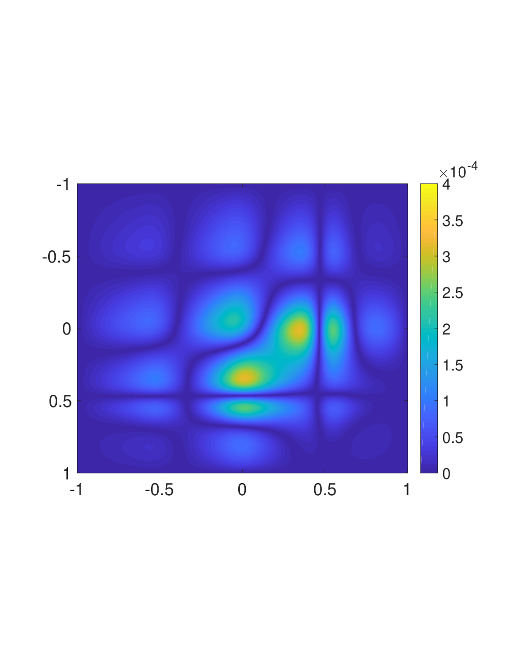
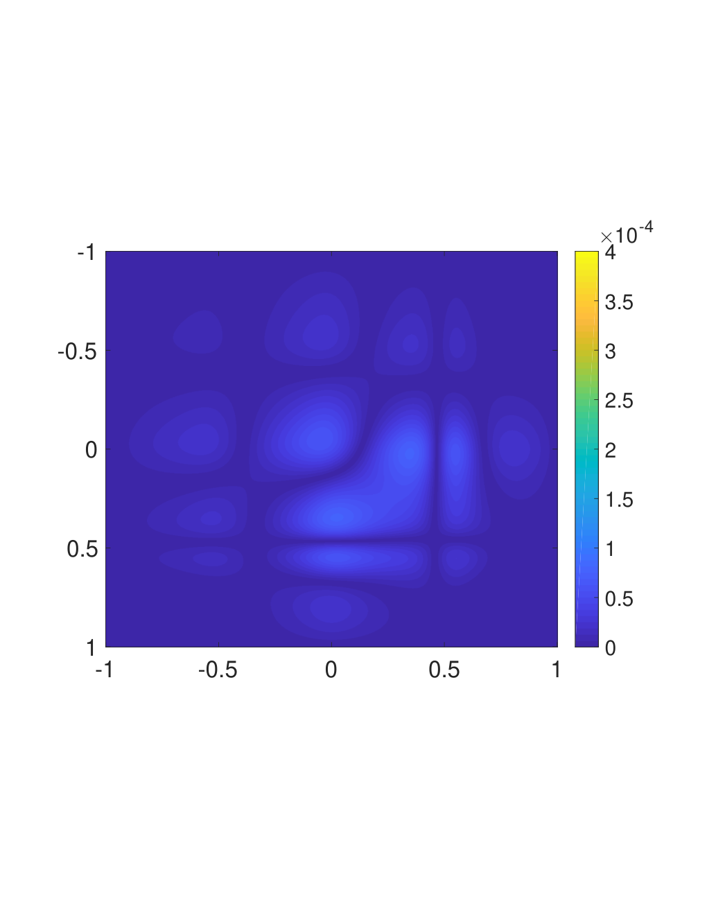
We observe that two columns in are localized far from the modified Gaussian, and we consider them as the bath orbitals. We set , this ensures . We then compute the linear PET problem to obtain , and we build the PET density matrix as shown in Fig. 6.3, which is accurate up to 3 digits in relative error. Furthermore, the error is mostly localized around the third Gaussian function as one would expect. The relative error of the energy is . We find it remarkable that for such a small system, the solution from PET is already very accurate despite the strong overlap of the system and bath orbitals.
Finally, we use Alg. 1 to compute the perturbed density matrix,, which is more accurate than the PET density matrix without the perturbation, , as depicted in Fig. 6.4. We can observe how the perturbation decreases the error in the density matrix by taking a look at the electron density, , in Fig. 6.5. In addition, the accuracy of the energy is improved, with its relative error reduced from to . If we increase the bath size from to , the accuracy of the energy is improved further to and , without and with the perturbative correction, respectively.


In order to showcase the asymptotic convergence of PET and the first order perturbation discussed at the end of Section 3, we introduce a family of perturbed Hamiltonians as
| (6.3) |
Then, in an analogous fashion as above, we compute the PET approximation and the associated perturbative correction for each Hamiltonian as . Fig. 6.6 (a) shows the error of approximation of the density matrix and the energy as the tends to zero. As discussed in Section 3, our first order perturbation is computed with respect to , which can remain to be of even if .
On the one hand, when we use localized orbitals to define the system and bath orbitals, Eq. (3.15) is not satisfied. In this case the error of the PET density matrix and energy decay as and , respectively as shown by Fig. 6.6 (a). Although, the asymptotic convergence after first order correction remains unchanged, the preconstants are significantly reduced by one to two orders of magnitude compared to the results of the PET.
On the other hand, when we use the delocalized eigenfunctions to define the system and bath orbitals, Eq. (3.15) is satisfied. In such a case, Fig. 6.6 (b) shows that the error of the approximate density matrix and energy after the perturbation correction decay as and , which agrees with results from the standard RS perturbation theory. However, the preconstants are larger than those in Fig. 6.6 (a). In particular, we can observe from Fig. 6.6 that when the perturbation is relatively large, partitioning the system with spatially localized orbitals indeed improves the accuracy of PET, specially when the perturbative correction is used.
6.2 Nonlinear Case
For KSDFT calculations, we modified the KSSOLV software package [36] to solve the PET equations (4.5) and to obtain the perturbation correction. KSSOLV uses a pseudo spectral discretization with the plane wave set. All the operators, including Hamiltonian and projection operators, are efficiently implemented in a matrix-free fashion. Within each self-consistent field iteration, we use the locally optimal block preconditioned conjugate gradient method (LOBPCG) [21] to solve the linear eigenvalue problems. For the perturbative correction, we use the GMRES [32] method with a preconditioner [34] implemented via fast Fourier transforms (FFTs).
6.2.1 Silane
We first consider a simple molecule, silane (SiH4), whose electron density in shown in Fig. 6.7 and we performed three different numerical experiments to showcase the accuracy of the method. Our reference system is the silane molecule from an equilibrium configuration. The bath-system partition is shown in Fig. 6.7, in which we can observe that we fixed three orbitals as the bath, induced by , and the system part, which is delimited by a pointed red line is considered as the forth orbital induced by . We performed three different modifications to the atom associated with the fourth orbital:


- •
we elongate one hydrogen bond by ,
- •
we replace a hydrogen atom by a chlorine atom (Cl),
- •
we replace a hydrogen atom by a fluorine atom (F).
Note that in the last two examples, the number of valence orbitals in the reference system is , while the number of valence orbitals in the perturbed systems are both . Hence the perturbation introduced by the atom substitution is very large, especially compared to the small size of the molecule under study here.
We compare the results from PET and the perturbed PET against a reference solution obtained directly by solving the system in KSSOLV. In particular, we examine the relative error of the density matrices, the relative error of the electron density, the absolute error of the energy, and the absolute error of the atomic force at the modified location. All results are reported in atomic units. In particular, the unit of the energy is hartree, and the unit of the atomic force is hartree / bohr. In this case, the energy for PET was computed using the functional in (4.4). For the perturbed solution, we used (4.6). We used a second order finite difference scheme to compute the forces at the perturbed atom.
The results for each of the experiments are shown in Tables 1 and 2. We can observe that the perturbation effectively reduces the error of the density matrix, the electron density, the energy and atomic force. The only exception is the force of SiH3F, which becomes coincidentally accurate for the PET, but the error after applying the perturbation theory is still around au. Even for such a small system, after applying the perturbation formula, the error of the energy and force already reaches chemical accuracy.
| Experiment | ||||
|---|---|---|---|---|
| Elongated | ||||
| SiH3Cl | ||||
| SiH3F |
| Experiment | ||||
|---|---|---|---|---|
| Elongated | ||||
| SiH3Cl | ||||
| SiH3F |
6.2.2 Benzene
In this example we show the performance of the method for a benzene molecule (C6H6), whose electron density is shown in Fig. 6.8 (a). We substitute one of hydrogen atoms by a fluorine atom, whose electron density is shown in Fig. 6.8 (b). The benzene molecule has a total of 15 valence orbitals. To determine the partitions, we created a sphere centered at the replaced atom and we performed the localization using Alg. 2 where we labeled the different localized orbitals depending on the position of their associated pivots (from Alg. 2). In particular, we labeled the orbitals whose pivots were within the sphere as system orbitals, and the rest as bath orbitals. The Tables 3 and 4 were generated by incrementally increasing the radius of the sphere, until obtaining system orbitals . The different partitions are depicted in Fig. 6.8, for and , in which the segmented red line indicates the boundary between the bath and system partitions. Tables 3 and 4 show the errors of the density matrix and the electron density, as well as the energy and the atomic force. We can observe a systematically decrease on the errors as the bath size decreases, i.e., , the system size increases. When the system size is , the error of the energy and force after perturbative correction is already below the chemical accuracy and is as small as and au, respectively.


| 1 | ||||
|---|---|---|---|---|
| 3 | ||||
| 5 | ||||
| 7 | ||||
| 9 |
| 1 | ||||
|---|---|---|---|---|
| 3 | ||||
| 5 | ||||
| 7 | ||||
| 9 | ||||
| 11 |
6.2.3 Anthracene
Finally we test our algorithm with the anthracene molecule (C14H10), which is composed of benzene rings positioned longitudinally. Following the same procedure as with the benzene molecule, we compute the solution to the Kohn-Sham equations, whose electron density is shown in Fig. 6.9 , and we replace one hydrogen atom in one of the extremal rings by a fluorine atom (Fig. 6.9 (b)). From the total 33 orbitals for the anthracene, we define the bath orbitals and systems orbitals following the same procedure as for the benzene molecule The partitions for and are depicted in Fig. 6.9, where the different segmented red lines indicate the boundary between the two partitions, in which they are denoted by and , for the bath and for the system respectively.
We compute the PET approximation and its perturbative correction for several different bath sizes as shown in Table 5. From Table 5 we can clearly observe the error of all quantities decrease systematically with respect to the increase of the system size, and the perturbation method significantly increases the accuracy over the PET results. In particular, when the system size is , chemical accuracy is achieved after the perturbative correction is applied.


| 1 | ||||
|---|---|---|---|---|
| 3 | ||||
| 5 | ||||
| 7 | ||||
| 9 | ||||
| 11 | ||||
| 13 | ||||
| 15 | ||||
| 19 |
| 1 | ||||
|---|---|---|---|---|
| 3 | ||||
| 5 | ||||
| 7 | ||||
| 9 | ||||
| 11 | ||||
| 13 | ||||
| 15 | ||||
| 19 |
7 Conclusion
We have studied the recently developed projection based embedding theory (PET) from a mathematical perspective. Viewed as a method to approximately solve eigenvalue problems, PET solves a deflated eigenvalue problem by taking into account the knowledge from a related reference system. This deflated eigenvalue problem can be derived from the Euler-Lagrange equation of a standard energy minimization procedure with respect to the density matrices, by with a non-standard constraint on the feasible set. From this perspective, the original formulation of PET can be seen as a penalty method for imposing the constraint. Numerical examples for linear problems as well as nonlinear problems from Kohn-Sham density functional theory calculations indicate that PET can yield accurate approximation to the density matrix, energy and atomic forces. In order to further improve the accuracy of PET, we developed a first order perturbation formula. We find that with the help of the perturbative treatment, PET can achieve chemical accuracy even for systems of relatively small sizes.
There are several immediate directions for future work. First, we have studied PET when the system and bath are treated using the same level of theory. From a physics perspective, it is more attractive to consider the case when the system part is treated with a more accurate theory than KSDFT with semi-local exchange-correlation functionals. In particular, it would be interesting to understand PET when the system part is treated using KSDFT with nonlocal functionals such as hybrid functionals, or wavefunction theories such as the coupled cluster (CC) method. It is also interesting to explore the PET in the context of solving time-dependent problems. Second, PET provides a size consistent alternative for many methods in quantum physics and chemistry to be applied to solid state systems. Some directions have already been pursued recently for using PET in the context of periodic systems [7, 26]. Third, the computation of the atomic force in PET is currently performed using the finite difference formula, which is expensive in practice. It would be desirable to develop a method with cost comparable to the Hellmann-Feynman method but without significant sacrifice of the accuracy. We note that there has been recent progress along this direction [24]. Finally, we believe that the asymptotic convergence property of PET is still dictated by the nearsightedness principle for systems satisfying the gap condition, but numerical results indicate that PET already achieves high accuracy even for system sizes that are well below the prediction from localization theories. Therefore it is worthwhile to further study the convergence properties of PET, as well as to perform further comparison with linear scaling type methods.
Acknowledgment
This work was partially supported by the Department of Energy under Grant No. DE-SC0017867, No. DE-AC02-05CH11231, the SciDAC program, and by the Air Force Office of Scientific Research under award number FA9550-18-1-0095 (L. L. and L. Z.-N.), and by the National Science Foundation under Grant No. DMS-1652330 (L. L.). We thank the Berkeley Research Computing (BRC) program at the University of California, Berkeley for making computational resources available. We thank Garnet Chan and Frederick Manby for discussions, and Joonho Lee for valuable suggestions and careful reading of the manuscript.
References
- [1] S. Baroni, S. de Gironcoli, A. Dal Corso, and P. Giannozzi, Phonons and related crystal properties from density-functional perturbation theory, Rev. Mod. Phys., 73 (2001), pp. 515–562.
- [2] M. Benzi, P. Boito, and N. Razouk, Decay properties of spectral projectors with applications to electronic structure, SIAM Rev., 55 (2013), pp. 3–64.
- [3] J. Bernholc, N. O. Lipari, and S. T. Pantelides, Self-consistent method for point defects in semiconductors: Application to the vacancy in silicon, Phys. Rev. Lett., 41 (1978), p. 895.
- [4] C. Brouder, G. Panati, M. Calandra, C. Mourougane, and N. Marzari, Exponential localization of Wannier functions in insulators, Phys. Rev. Lett., 98 (2007), p. 046402.
- [5] H. Chen and C. Ortner, QM/MM methods for crystalline defects. Part 2: Consistent energy and force-mixing, arXiv:1509.06627, (2015).
- [6] W. Chibani, X. Ren, M. Scheffler, and P. Rinke, Self-consistent Green’s function embedding for advanced electronic structure methods based on a dynamical mean-field concept, Phys. Rev. B, 93 (2016), p. 165106.
- [7] D. V. Chulhai and J. D. Goodpaster, Projection-based correlated wave function in density functional theory embedding for periodic systems, J. Chem. Theory Comput., 14 (2018), pp. 1928–1942.
- [8] P. Cortona, Self-consistently determined properties of solids without band-structure calculations, Phys. Rev. B, 44 (1991), p. 8454.
- [9] A. Damle, L. Lin, and L. Ying, Compressed representation of Kohn–Sham orbitals via selected columns of the density matrix, J. Chem. Theory Comput., 11 (2015), pp. 1463–1469.
- [10] A. Damle, L. Lin, and L. Ying, Accelerating selected columns of the density matrix computations via approximate column selection, SIAM J. Sci. Comput., 39 (2017), p. 1178.
- [11] J. M. Foster and S. F. Boys, Canonical configurational interaction procedure, Rev. Mod. Phys., 32 (1960), p. 300.
- [12] C.J. García-Cervera, J. Lu, and W. E, Asymptotics-based sub-linear scaling algorithms and application to the study of the electronic structure of materials, Commun. Math. Sci., 5 (2007), pp. 999–1024.
- [13] G. H. Golub and C. F. Van Loan, Matrix computations, Johns Hopkins Univ. Press, Baltimore, fourth ed., 2013.
- [14] J. D. Goodpaster, N. Ananth, F. R. Manby, and T. F. Miller III, Exact nonadditive kinetic potentials for embedded density functional theory, J. Chem. Phys., 133 (2010), p. 084103.
- [15] P. Hohenberg and W. Kohn, Inhomogeneous electron gas, Phys. Rev., 136 (1964), pp. B864–B871.
- [16] C. Huang, M. Pavone, and E. A. Carter, Quantum mechanical embedding theory based on a unique embedding potential, J. Chem. Phys., 134 (2011), p. 154110.
- [17] S. Huzinaga and A. A. Cantu, Theory of separability of many electron systems, J. Chem. Phys., 55 (1971), pp. 5543–5549.
- [18] A. A. Kananenka, E. Gull, and D. Zgid, Systematically improvable multiscale solver for correlated electron systems, Phys. Rev. B, 91 (2015), p. 121111.
- [19] P. J. Kelly and R. Car, Green’s-matrix calculation of total energies of point defects in silicon, Phys. Rev. B, 45 (1992), p. 6543.
- [20] G. Knizia and G. K.-L. Chan, Density matrix embedding: A strong-coupling quantum embedding theory, J. Chem. Theory Comput., 9 (2013), pp. 1428–1432.
- [21] A. V. Knyazev, Toward the optimal preconditioned eigensolver: Locally optimal block preconditioned conjugate gradient method, SIAM J. Sci. Comp., 23 (2001), pp. 517–541.
- [22] W. Kohn, Density functional and density matrix method scaling linearly with the number of atoms, Phys. Rev. Lett., 76 (1996), pp. 3168–3171.
- [23] W. Kohn and L. Sham, Self-consistent equations including exchange and correlation effects, Phys. Rev., 140 (1965), pp. A1133–A1138.
- [24] S.J.R. Lee, F. Ding, F.R. Manby, and T.F. Miller III, Analytical Gradients for Projection-Based Wavefunction-in-DFT Embedding, arXiv:1903.05830, (2019).
- [25] X. Li, L. Lin, and J. Lu, PEXSI-: A Green’s function embedding method for Kohn-Sham density functional theory, Ann. Math. Sci. Appl., 3 (2018), p. 411.
- [26] F. Libisch, M. Marsman, J. Burgdörfer, and G. Kresse, Embedding for bulk systems using localized atomic orbitals, J. Chem. Phys., 147 (2017), p. 034110.
- [27] X. Liu, Z. Wen, X. Wang, M. Ulbrich, and Y. Yuan, On the analysis of the discretized Kohn–Sham density functional theory, SIAM J. Numer. Anal., 53 (2015), pp. 1758–1785.
- [28] F. R. Manby, M. Stella, J. D. Goodpaster, and T. F. Miller III, A simple, exact density-functional-theory embedding scheme, J. Chem. Theory Comput., 8 (2012), pp. 2564–2568.
- [29] N. Marzari and D. Vanderbilt, Maximally localized generalized Wannier functions for composite energy bands, Phys. Rev. B, 56 (1997), p. 12847.
- [30] T. Nguyen, A. A. Kananenka, and D. Zgid, Rigorous ab initio quantum embedding for quantum chemistry using Green’s function theory: Screened interaction, nonlocal self-energy relaxation, orbital basis, and chemical accuracy, J. Chem. Theory Comput., (2016).
- [31] E. Prodan and W. Kohn, Nearsightedness of electronic matter, Proc. Natl. Acad. Sci., 102 (2005), pp. 11635–11638.
- [32] Y. Saad and M. H. Schultz, GMRES: A generalized minimal residual algorithm for solving nonsymmetric linear systems, SIAM J. Sci. Stat. Comput., 7 (1986), pp. 856–869.
- [33] Q. Sun and G. K.-L. Chan, Quantum embedding theories, Acc. Chem. Res., 49 (2016), pp. 2705–2712.
- [34] M.P. Teter, M.C. Payne, and D.C. Allan, Solution of Schrödinger’s equation for large systems, Phys. Rev. B, 40 (1989), p. 12255.
- [35] A. R. Williams, P. J. Feibelman, and N. D. Lang, Green’s-function methods for electronic-structure calculations, Phys. Rev. B, 26 (1982), p. 5433.
- [36] C. Yang, J. C. Meza, B. Lee, and L. W. Wang, KSSOLV–a MATLAB toolbox for solving the Kohn–Sham equations, ACM Trans. Math. Software, 36 (2009), p. 10.
- [37] R. Zeller and P. H. Dederichs, Electronic Structure of Impurities in Cu, Calculated Self-Consistently by Korringa-Kohn-Rostoker Green’s-Function Method, Phys. Rev. Lett., 42 (1979), p. 1713.
- [38] D. Zgid and G. K.-L. Chan, Dynamical mean-field theory from a quantum chemical perspective, J. Chem. Phys., 134 (2011), p. 094115.