跳到论文正文
W Papers独立论文阅读器 arXiv:1807.08697 论文正文 计算阅读时间 · 0%
引用这篇论文根据当前论文元数据生成,正式投稿前建议核对。


License: arXiv.org perpetual non-exclusive license
arXiv:1807.08697v1 [hep-ph] 23 Jul 2018

Probing the Weizs𝐚¨\ddot{{\bf a}}cker-Williams gluon Wigner distribution in p​ppp collisions

Preprint: YITP-18-67
Renaud Boussarie Affiliation: Institute of Nuclear Physics, Polish Academy of Sciences, Radzikowskiego 152, PL-31-342 Krako´\acute{o}w, Poland    Yoshitaka Hatta Affiliation: Yukawa Institute for Theoretical Physics, Kyoto University, Kyoto 606-8502, Japan    Bo-Wen Xiao Affiliation: Key Laboratory of Quark and Lepton Physics (MOE) and Institute of Particle Physics, Central China Normal University, Wuhan 430079, China Affiliation: Centre de Physique Théorique, École Polytechnique, CNRS, Université Paris-Saclay, Route de Saclay, 91128 Palaiseau, France.    Feng Yuan Affiliation: Nuclear Science Division, Lawrence Berkeley National Laboratory, Berkeley, CA 94720, USA
Abstract

We show that the diffractive forward production of two quarkonia, especially the χc​J\chi_{cJ} and ηc\eta_{c} states, in proton-proton or proton-ion collisions can access the Weizsa¨\ddot{{\rm a}}cker-Williams gluon Wigner distribution of the proton. We use the hybrid factorization approach where the collinear, double gluon PDF is applied for one of the protons and the kTk_{T}-dependent (Wigner or GTMD) distribution for the other. The production of quarkonia is treated in the NRQCD framework. A particularly concise formula is obtained for double χJ=1\chi_{J=1} production.

pacs
24.85.+p, 12.38.Bx, 14.20.Dh

I Introduction

In hadron physics research, one of the ultimate goals is to depict the colorful and kaleidoscopic multi-dimensional landscape of the internal structure of hadrons including nucleons and nucleus. In particular, in addition to the longitudinal momentum distribution of partons inside hadrons as given by the Feynman parton distributions, we also intend to learn about the transverse spatial (generalized parton distributions (GPD)) and transverse momentum (transverse momentum dependent (TMD)) distributions. The so-called quantum phase space Wigner distributions [1, 2, 3] encode all the above important informations and are viewed as the mother distributions of all. In practice, since it is rather difficult to directly measure the spatial transverse coordinates in high energy scatterings, we also normally define the generalized transverse momentum distribution (GTMD)[4, 5, 6] as the Fourier transform of the corresponding Wigner distribution for quarks and gluons.

Interestingly, as pointed out in Refs. [7, 8, 9, 10, 11], quark and gluon TMDs are not unique due to different possible structures of gauge links representing the initial and final state interactions. As far as the gluon TMDs are concerned, there are at least two nontrivial gluon distributions whose difference becomes crucial especially in the small-xx region. One is known as the dipole gluon distribution which contains the dipole-shaped configuration of gauge links, while the other is called the Weizsa¨\ddot{{\rm a}}cker-Williams (WW) gluon distribution which features either a future-pointing or past-pointing gauge link, but not both. Naturally, one expects that this kind of complication should also persist in the case of Wigner distributions and GTMDs.

Generally speaking, up to now, the HERA experiment has provided us with the most precise knowledge of Feynman parton distributions for a large range of xx region, through the inclusive deep inelastic scattering (DIS) process. Furthermore, less inclusive processes, such as the semi-inclusive DIS (SIDIS) and the deeply virtual Compton scattering (DVCS) can help us gain insights on the TMDs and GPDs, respectively. The important question here is whether one can probe the Wigner distributions or GTMDs experimentally. It is rather challenging to achieve such a goal because, obviously, one has to consider more exclusive/complicated processes than SIDIS and DVCS.

Recently, we have found that the goal of measuring the gluon Wigner distributions can be achieved at the future electron-hadron colliders [12], such as the planned electron-ion colliders (EIC) and the large hadron electron collider (LHeC) [13, 14, 15]. Specifically, the dipole gluon Wigner or GTMD can be probed in diffractive dijet process in the small-xx region at EIC [16]. Subsequently, there have been a lot of progress on this topic in the last two years [17, 18, 19, 20, 21, 22, 23, 24, 25, 26, 27, 28]. Especially, one can access and study the extremely evasive gluon orbital angular momentum with the help of the spin-dependent gluon GTMD as discussed in Refs. [29, 30, 20, 21, 23, 31, 27].

On the other hand, it has been realized already in Ref. [12] that the Weizs𝐚¨\ddot{{\bf a}}cker-Williams Wigner (WWW) distribution is more difficult to access. One possibility, as suggested in [12], was to look at a process involving two incoming photons and four outgoing jets at EIC. However, the transition rate would be too small to make it a realistic measurement. The objective of this paper is to show that it is possible to rather directly probe the WWW distribution and WW type GTMD for small-xx gluons in the production of two heavy scalar quarkonia such as χc\chi_{c} and ηc\eta_{c} in the forward rapidity region in diffractive p​ppp and p​ApA collisions p​p,p​A→χc​χc​p​Xpp,pA\to\chi_{c}\chi_{c}pX.

The rest of the paper is organized as follows. We first introduce the WW gluon GTMD and briefly describe the process we will consider in this paper, i.e., double quarkonia production in the hard diffractive processes in p​ppp and p​ApA collisions. In Sec. III, we derived the amplitude for the double quarkonia production through double gluon scattering on the nucleon/nucleus targets. These amplitudes will be converted into p​ppp/p​ApA collisions cross sections in Sec. IV by applying the double parton scattering framework for the incoming two gluons from the projectile. In Sec.III and IV, we derive the results for both η\eta and χ\chi. In particular, we will present the explicit differential cross sections on different combinations of two quarkonia states of η\eta, χ0,1,2\chi_{0,1,2}. Finally, we summarize our paper in Sec. VI.

II Weizs𝐀¨\ddot{{\bf A}}cker-Williams gluon GTMD

We start by writing down the Weizsa¨\ddot{{\rm a}}cker-Williams (WW) gluon GTMD. For the ‘target’ proton fast-moving in the negative zz-direction we define

x𝒢i​j(𝑲,𝚫)≡2∫d3​zP−​(2​π)3ei​x​P−​z+−i​𝑲⋅𝒛⟨P−Δ2|Tr[U±†F−i(z/2)U±F−j(−z/2)]|P+Δ2⟩,x\mathcal{G}^{ij}\left(\boldsymbol{K},\boldsymbol{\Delta}\right)\equiv 2\int\frac{d^{3}z}{P^{-}\left(2\pi\right)^{3}}e^{ixP^{-}z^{+}-i\boldsymbol{K}\cdot\boldsymbol{z}}\left\langle P-\frac{\Delta}{2}\left|\mathrm{Tr}\left[U^{\dagger}_{\pm}F^{-i}(z/2)U_{\pm}F^{-j}(-z/2)\right]\right|P+\frac{\Delta}{2}\right\rangle, (1)

where U±U_{\pm} is the staple-shaped fundamental Wilson line connecting the points z/2z/2 and −z/2-z/2 via light-like Wilson lines encircling x+=±∞x^{+}=\pm\infty. Boldface letters denote two-dimensional vectors. We have kept the transverse indices i,j=1,2i,j=1,2 open because this is what we shall need in later calculations. In the small-xx region, we may approximate ei​x​P−​z+≈1e^{ixP^{-}z^{+}}\approx 1 and find (c.f., [11])

x𝒢i​j(𝑲,𝚫)≈−2αs∫d2​𝒃1​d2​𝒃2(2​π)4e−i𝚫⋅𝒃1+𝒃22−i𝑲⋅(𝒃1−𝒃2)⟨P−Δ2​|Tr⁡[(∂iU𝒃1†)​U𝒃1​(∂jU𝒃2†)​U𝒃2]|​P+Δ2⟩⟨P|P⟩,x\mathcal{G}^{ij}\left(\boldsymbol{K},\boldsymbol{\Delta}\right)\approx-\frac{2}{\alpha_{s}}\int\frac{d^{2}\boldsymbol{b}_{1}d^{2}\boldsymbol{b}_{2}}{\left(2\pi\right)^{4}}e^{-i\boldsymbol{\Delta}\cdot\frac{\boldsymbol{b}_{1}+\boldsymbol{b}_{2}}{2}-i\boldsymbol{K}\cdot\left(\boldsymbol{b}_{1}-\boldsymbol{b}_{2}\right)}\frac{\left\langle P-\frac{\Delta}{2}\left|\mathrm{Tr}\left[\left(\partial^{i}U_{\boldsymbol{b}_{1}}^{\dagger}\right)U_{\boldsymbol{b}_{1}}\left(\partial^{j}U_{\boldsymbol{b}_{2}}^{\dagger}\right)U_{\boldsymbol{b}_{2}}\right]\right|P+\frac{\Delta}{2}\right\rangle}{\left\langle P|P\right\rangle}, (2)

where U𝒃U_{\boldsymbol{b}} is the lightlike Wilson line from x+=−∞x^{+}=-\infty to x+=+∞x^{+}=+\infty at fixed transverse position 𝒃\boldsymbol{b}. It is easy to check from (2) the relations 𝒢i​j​(𝑲,𝚫)=𝒢j​i​(−𝑲,𝚫)=(𝒢i​j​(−𝑲,−𝚫))∗\mathcal{G}^{ij}\left(\boldsymbol{K},\boldsymbol{\Delta}\right)=\mathcal{G}^{ji}\left(-\boldsymbol{K},\boldsymbol{\Delta}\right)=(\mathcal{G}^{ij}(-\boldsymbol{K},-\boldsymbol{\Delta}))^{*}. The general parameterization is thus11 1 Naively, there is another term proportional to the tensor structure 𝑲i​𝚫j+𝑲j​𝚫i−𝑲⋅𝚫​δi​j\boldsymbol{K}^{i}\boldsymbol{\Delta}^{j}+\boldsymbol{K}^{j}\boldsymbol{\Delta}^{i}-\boldsymbol{K}\cdot\boldsymbol{\Delta}\delta^{ij}. However, as pointed out in [32], this term is not independent and can be absorbed in 𝒢2,3{\cal G}_{2,3}. See, also, [5].

𝒢i​j​(𝑲,𝚫)≡δi​j​𝒢1+(𝑲i​𝑲j𝑲2−δi​j2)​𝑲2M2​𝒢2+(𝚫i​𝚫j𝚫2−δi​j2)​𝚫2M2​𝒢3+(𝑲i​𝚫j−𝚫i​𝑲jM2)​𝒢4,\mathcal{G}^{ij}\left(\boldsymbol{K},\boldsymbol{\Delta}\right)\equiv\delta^{ij}\mathcal{G}_{1}+\left(\frac{\boldsymbol{K}^{i}\boldsymbol{K}^{j}}{\boldsymbol{K}^{2}}-\frac{\delta^{ij}}{2}\right)\frac{\boldsymbol{K}^{2}}{M^{2}}\mathcal{G}_{2}+\left(\frac{\boldsymbol{\Delta}^{i}\boldsymbol{\Delta}^{j}}{\boldsymbol{\Delta}^{2}}-\frac{\delta^{ij}}{2}\right)\frac{\boldsymbol{\Delta}^{2}}{M^{2}}\mathcal{G}_{3}+\left(\frac{\boldsymbol{K}^{i}\boldsymbol{\Delta}^{j}-\boldsymbol{\Delta}^{i}\boldsymbol{K}^{j}}{M^{2}}\right)\mathcal{G}_{4}, (3)

where MM is the nucleon mass. 𝒢1,2,3,4{\cal G}_{1,2,3,4} are all real and depend on 𝑲2\boldsymbol{K}^{2}, 𝚫2\boldsymbol{\Delta}^{2} and (𝑲⋅𝚫)2(\boldsymbol{K}\cdot\boldsymbol{\Delta})^{2}. In the forward limit 𝚫=0\boldsymbol{\Delta}=0, 𝒢1{\cal G}_{1} and 𝒢2{\cal G}_{2} reduce to the unpolarized and linearly polarized WW gluon TMDs, respectively. The 𝑲\boldsymbol{K}-integral of 𝒢3{\cal G}_{3} is proportional to the gluon transversity GPD which in turn is related to the so-called elliptic gluon Wigner distribution [24]. From what we know about the latter distribution [12, 18, 22], we presume that 𝒢3{\cal G}_{3} is numerically small, on the order of a few percent effect compared to 𝒢1,2{\cal G}_{1,2}.

Various experimental processes have been identified to probe the WW gluon TMD [11]. On the other hand, the measurement of the GTMDs is more challenging, and most of the proposals so far concern the dipole gluon GTMD whose treatment is somewhat simpler because of its relation to the dipole S-matrix [12]. In this paper, we show that double quarkonium production in p​ppp collisions p​p→M1​M2​p​Xpp\to M_{1}M_{2}pX is a very sensitive observable for the WW gluon GTMD. This is a natural extension of the previous observation [34] (see, also, [33]) that the WW gluon TMD can be probed in single quarkonium production p​p→M​Xpp\to MX. The hard subprocess and the full process are respectively depicted in Fig. 1 and in Fig. 3. Two gluons are emitted from the projectile proton and scatter off the shockwave field created by the target proton. In the final state, we measure two quarkonia with momentum K1K_{1} and K2K_{2} in the forward region as well as the elastically scattered target with momentum transfer 𝚫=𝑲1+𝑲2\boldsymbol{\Delta}=\boldsymbol{K}_{1}+\boldsymbol{K}_{2} in the backward region. To lowest order, the shockwave consists of two gluons in the tt-channel, and we can view this diagram as the square of the g​g∗→Mgg^{*}\to M amplitude. This means that the produced quarkonia must be CC-even states, such as ηc\eta_{c} and χc​J\chi_{cJ} (and their bottomonium counterparts). We study this process in the ‘hybrid factorization’ approach (collinear gluons from one proton and non-collinear gluons from the other proton) and show that the cross section can be written as a convolution of the square of the WW gluon GTMD of the target and the double gluon PDF of the projectile.

It should be mentioned that a very similar idea came out recently in Ref. [31] where the authors proposed to measure the gluon GTMD (including its spin dependence) in doubly-diffractive double ηc\eta_{c} production p​p→p​p​ηc​ηcpp\to pp\eta_{c}\eta_{c} for moderate values of xx. Their argument is limited to the two-gluon exchange level where the difference between WW and dipole distributions becomes immaterial. Our process is single-diffractive and we do not consider spin effects. Instead, we focus on the forward, small-xx region and carefully examine the structure of the relevant Wilson lines. Our result suggests that the GTMD discussed in [31] likely becomes the WW GTMD once higher order rescattering effects are taken into account.

Refer to caption
Figure 1: Production of 2 quarkonia from 2 gluons

III Quarkonium production amplitude

III.1 Single quarkonium production

As a warm-up, we first compute the amplitude for the single quarkonium production in the hybrid factorization approach combined with the non-relativistic QCD (NRQCD) framework. Related calculations can be found in the literature, e.g., [34, 33]. The right-moving projectile proton is treated as a dilute object, i.e. partons are extracted from the projectile using regular Parton Distribution Functions, whereas the left-moving target is treated as a showckwave. The subamplitude for the open production of a massive q​q¯q\bar{q} pair from a gluon (see Fig. 2) can be straightfowardly written as, in D=d+2D=d+2 dimensions,22 2 Our notation is as follows: We define two lightlike vectors n1,n2n_{1},n_{2} such that the projectile flies along n1n_{1} and the target flies along n2n_{2}, and such that n1⋅n2=1n_{1}\cdot n_{2}=1. Lightcone coordinates are then defined as kμ\displaystyle k^{\mu} ≡\displaystyle\equiv k+​n1μ+k−​n2μ+k⟂μ,\displaystyle k^{+}n_{1}^{\mu}+k^{-}n_{2}^{\mu}+k_{\perp}^{\mu}, (4) k⋅l\displaystyle k\cdot l ≡\displaystyle\equiv k+​l−+k−​l++k⟂⋅l⟂≡k+​l−+k−​l+−(𝒌⋅𝒍).\displaystyle k^{+}l^{-}+k^{-}l^{+}+k_{\perp}\cdot l_{\perp}\equiv k^{+}l^{-}+k^{-}l^{+}-(\boldsymbol{k}\cdot\boldsymbol{l}). (5) The metric tensor will be decomposed into its longitudinal and transverse parts as gμ​ν\displaystyle g^{\mu\nu} ≡\displaystyle\equiv n1μ​n2ν+n1ν​n2μ+g⟂μ​ν.\displaystyle n_{1}^{\mu}n_{2}^{\nu}+n_{1}^{\nu}n_{2}^{\mu}+g_{\perp}^{\mu\nu}. (6)

(𝒜σ)c\displaystyle\left(\mathcal{A}_{\sigma}\right)^{c} =\displaystyle= −ig∫dDz0u¯(pq,z0)γμtbεμc​b(k,z0)v(pq¯,z0),\displaystyle-ig\int d^{D}z_{0}\bar{u}\left(p_{q},z_{0}\right)\gamma^{\mu}t^{b}\varepsilon_{\mu}^{cb}\left(k,z_{0}\right)v\left(p_{\bar{q}},z_{0}\right), (7)

where, with similar methods as in [35, 36] one can derive the effective quark, antiquark and gluon lines as obtained for example in [37, 17]:

u¯​(pq,z0)\displaystyle\bar{u}\left(p_{q},\,z_{0}\right) =\displaystyle= 12​(pq+2​π)d2​∫dd​𝒙1​ei​pq+​(z0−−(𝒙1−𝒛0)22​z0++i​0)−i​𝒑q⋅𝒙1+i​z0+2​pq+​(m2+i​0)\displaystyle\frac{1}{2}\left(\frac{p_{q}^{+}}{2\pi}\right)^{\frac{d}{2}}\int d^{d}\boldsymbol{x}_{1}e^{ip_{q}^{+}\left(z_{0}^{-}-\frac{\left(\boldsymbol{x}_{1}-\boldsymbol{z}_{0}\right)^{2}}{2z_{0}^{+}}+i0\right)-i\boldsymbol{p}_{q}\cdot\boldsymbol{x}_{1}+i\frac{z_{0}^{+}}{2p_{q}^{+}}\left(m^{2}+i0\right)}
×(iz0+)d2​u¯pq​γ+​[U𝒙1​θ​(−z0+)+θ⁡(z0+)]​(γ−−x1⟂−z0⟂z0++mpq+),\displaystyle\times\left(\frac{i}{z_{0}^{+}}\right)^{\frac{d}{2}}\bar{u}_{p_{q}}\gamma^{+}\left[U_{\boldsymbol{x}_{1}}\theta\left(-z_{0}^{+}\right)+\theta\left(z_{0}^{+}\right)\right]\left(\gamma^{-}-\frac{{\vtop{\halign{#\cr\hfil/\hfil\crcr$x$\crcr}}}_{1\perp}-{\vtop{\halign{#\cr\hfil/\hfil\crcr$z$\crcr}}}_{0\perp}}{z_{0}^{+}}+\frac{m}{p_{q}^{+}}\right),
v⁡(pq¯,z0)\displaystyle v\left(p_{\bar{q}},\,z_{0}\right) =\displaystyle= 12​(pq¯+2​π)d2​∫dd​𝒙2​ei​pq¯+​(z0−−(𝒙2−𝒛0)22​z0++i​0)−i​𝒑q¯⋅𝒙2+i​z0+2​pq¯+​(m2+i​0)\displaystyle\frac{1}{2}\left(\frac{p_{\bar{q}}^{+}}{2\pi}\right)^{\frac{d}{2}}\int d^{d}\boldsymbol{x}_{2}e^{ip_{\bar{q}}^{+}\left(z_{0}^{-}-\frac{\left(\boldsymbol{x}_{2}-\boldsymbol{z}_{0}\right)^{2}}{2z_{0}^{+}}+i0\right)-i\boldsymbol{p}_{\bar{q}}\cdot\boldsymbol{x}_{2}+i\frac{z_{0}^{+}}{2p_{\bar{q}}^{+}}\left(m^{2}+i0\right)}
×(iz0+)d2​(γ−−x2⟂−z0⟂z0+−mpq¯+)​[U𝒙2†​θ​(−z0+)+θ⁡(z0+)]​γ+​vpq¯,\displaystyle\times\left(\frac{i}{z_{0}^{+}}\right)^{\frac{d}{2}}\left(\gamma^{-}-\frac{{\vtop{\halign{#\cr\hfil/\hfil\crcr$x$\crcr}}}_{2\perp}-{\vtop{\halign{#\cr\hfil/\hfil\crcr$z$\crcr}}}_{0\perp}}{z_{0}^{+}}-\frac{m}{p_{\bar{q}}^{+}}\right)\left[U_{\boldsymbol{x}_{2}}^{\dagger}\theta\left(-z_{0}^{+}\right)+\theta\left(z_{0}^{+}\right)\right]\gamma^{+}v_{p_{\bar{q}}},
εμb​a​(k,z0)\displaystyle\varepsilon_{\mu}^{ba}\left(k,\,z_{0}\right) =\displaystyle= (k+2​π)d2​∫dd​𝒙0​e−i​k+​(z0−−(𝒙0−𝒛0)22​z0+−i​0)+i​𝒌⋅𝒙0\displaystyle\left(\frac{k^{+}}{2\pi}\right)^{\frac{d}{2}}\int d^{d}\boldsymbol{x}_{0}e^{-ik^{+}\left(z_{0}^{-}-\frac{\left(\boldsymbol{x}_{0}-\boldsymbol{z}_{0}\right)^{2}}{2z_{0}^{+}}-i0\right)+i\boldsymbol{k}\cdot\boldsymbol{x}_{0}} (18)
×(−iz0+)d2​(g⟂μ​σ+x0⟂σ−z0⟂σz0+​n2​μ)​[U𝒙0b​a​θ​(z0+)+δa​b​θ​(−z0+)]​εk⟂σ.\displaystyle\times\left(\frac{-i}{z_{0}^{+}}\right)^{\frac{d}{2}}\left(g_{\perp\mu\sigma}+\frac{x_{0\perp\sigma}-z_{0\perp\sigma}}{z_{0}^{+}}n_{2\mu}\right)\left[U_{\boldsymbol{x}_{0}}^{ba}\theta\left(z_{0}^{+}\right)+\delta^{ab}\theta\left(-z_{0}^{+}\right)\right]\varepsilon_{k\perp}^{\sigma}.

In the above, mm is the heavy quark mass and we have kept the transverse momentum of the incoming gluon 𝒌\boldsymbol{k}. UU is the Wilson line which arises after the eikonal interaction with the target field A−A^{-}

U𝒙\displaystyle U_{\boldsymbol{x}} ≡\displaystyle\equiv 𝒫​ei​g​∫−∞∞d​x+​A−​(x),\displaystyle\mathcal{P}e^{ig\int_{-\infty}^{\infty}dx^{+}A^{-}(x)}, (19)

We will use the conventions that lines with color indices as superscrispts U𝒙a​bU_{\boldsymbol{x}}^{ab} are in the adjoint representation while lines without color indices are in the fundamental representation.

Refer to caption
Figure 2: Open charm production

Integrating over the interaction point z0z_{0}, we get

(𝒜σ)c=εk⟂σ​u¯pq​ℳσc​vpq¯,\displaystyle\left(\mathcal{A}_{\sigma}\right)^{c}=\varepsilon_{k\perp}^{\sigma}\bar{u}_{p_{q}}\mathcal{M}_{\sigma}^{c}v_{p_{\bar{q}}}, (20)

where

ℳσc\displaystyle\mathcal{M}_{\sigma}^{c} =\displaystyle= −i​g2​(2​π)​δ​(pq++pq¯+−k+)​(pq+​pq¯+​k+2​π)d2\displaystyle-\frac{ig}{2}\left(2\pi\right)\delta\left(p_{q}^{+}+p_{\bar{q}}^{+}-k^{+}\right)\left(\frac{p_{q}^{+}p_{\bar{q}}^{+}k^{+}}{2\pi}\right)^{\frac{d}{2}}
×∫dd𝒙1dd𝒙2dd𝒙0e−i𝒑q⋅𝒙1−i𝒑q¯⋅𝒙2+i𝒌⋅𝒙0δ(pq+𝒙1+pq¯+𝒙2−k+𝒙0)\displaystyle\times\int d^{d}\boldsymbol{x}_{1}d^{d}\boldsymbol{x}_{2}d^{d}\boldsymbol{x}_{0}e^{-i\boldsymbol{p}_{q}\cdot\boldsymbol{x}_{1}-i\boldsymbol{p}_{\bar{q}}\cdot\boldsymbol{x}_{2}+i\boldsymbol{k}\cdot\boldsymbol{x}_{0}}\delta\left(p_{q}^{+}\boldsymbol{x}_{1}+p_{\bar{q}}^{+}\boldsymbol{x}_{2}-k^{+}\boldsymbol{x}_{0}\right)
×[1z0+​(γ⟂σ​x12⟂−2​pq¯+k+​x12⟂σ)−m​k+pq+​pq¯+​γ⟂σ]​γ+\displaystyle\times\left[\frac{1}{z_{0}^{+}}\left(\gamma_{\perp\sigma}{\vtop{\halign{#\cr\hfil/\hfil\crcr$x$\crcr}}}_{12\perp}-2\frac{p_{\bar{q}}^{+}}{k^{+}}x_{12\perp\sigma}\right)-m\frac{k^{+}}{p_{q}^{+}p_{\bar{q}}^{+}}\gamma_{\perp\sigma}\right]\gamma^{+}
×[(−i)d2∫−∞0dz0+(−z0+)−d2(U𝒙1tcU𝒙2†)ei​k+​(m2−i​0)2​pq+​pq¯+​z0+−i​pq+​pq¯+​𝒙1222​k+​1+i​0z0+\displaystyle\times\left[\left(-i\right)^{\frac{d}{2}}\int_{-\infty}^{0}dz_{0}^{+}\left(-z_{0}^{+}\right)^{-\frac{d}{2}}\left(U_{\boldsymbol{x}_{1}}t^{c}U_{\boldsymbol{x}_{2}}^{\dagger}\right)e^{i\frac{k^{+}\left(m^{2}-i0\right)}{2p_{q}^{+}p_{\bar{q}}^{+}}z_{0}^{+}-i\frac{p_{q}^{+}p_{\bar{q}}^{+}\boldsymbol{x}_{12}^{2}}{2k^{+}}\frac{1+i0}{z_{0}^{+}}}\right.
+id2∫0+∞dz0+(z0+)−d2(tdU𝒙0c​d)ei​k+​(m2+i​0)2​pq+​pq¯+​z0+−i​pq+​pq¯+​𝒙1222​k+​1−i​0z0+].\displaystyle\left.+i^{\frac{d}{2}}\int_{0}^{+\infty}dz_{0}^{+}\left(z_{0}^{+}\right)^{-\frac{d}{2}}\left(t^{d}U_{\boldsymbol{x}_{0}}^{cd}\right)e^{i\frac{k^{+}\left(m^{2}+i0\right)}{2p_{q}^{+}p_{\bar{q}}^{+}}z_{0}^{+}-i\frac{p_{q}^{+}p_{\bar{q}}^{+}\boldsymbol{x}_{12}^{2}}{2k^{+}}\frac{1-i0}{z_{0}^{+}}}\right].

Using the integrals, for Q,Z>0Q,Z>0:

∫−∞0d​z+​(−z+)−n​ei⁡(Q−i​0)​z+−i​Z+i​0z+\displaystyle\int_{-\infty}^{0}dz^{+}\left(-z^{+}\right)^{-n}e^{i\left(Q-i0\right)z^{+}-i\frac{Z+i0}{z^{+}}} =\displaystyle= 2​(−i)1−n​(ZQ)1−n​Kn−1​(2​Q​Z)\displaystyle 2\left(-i\right)^{1-n}\left(\sqrt{\frac{Z}{Q}}\right)^{1-n}K_{n-1}\left(2\sqrt{QZ}\right)
∫0+∞d​z+​(z+)−n​ei⁡(Q+i​0)​z+−i​Z−i​0z+\displaystyle\int_{0}^{+\infty}dz^{+}\left(z^{+}\right)^{-n}e^{i\left(Q+i0\right)z^{+}-i\frac{Z-i0}{z^{+}}} =\displaystyle= 2​i1−n​(ZQ)1−n​Kn−1​(2​Q​Z),\displaystyle 2i^{1-n}\left(\sqrt{\frac{Z}{Q}}\right)^{1-n}K_{n-1}\left(2\sqrt{QZ}\right),

we get

ℳσc\displaystyle\mathcal{M}_{\sigma}^{c} =\displaystyle= igδ(pq++pq¯+−k+)∫dd𝒙1dd𝒙2dd𝒙0e−i𝒑q⋅𝒙1−i𝒑q¯⋅𝒙2+i𝒌⋅𝒙0\displaystyle ig\delta\left(p_{q}^{+}+p_{\bar{q}}^{+}-k^{+}\right)\int d^{d}\boldsymbol{x}_{1}d^{d}\boldsymbol{x}_{2}d^{d}\boldsymbol{x}_{0}e^{-i\boldsymbol{p}_{q}\cdot\boldsymbol{x}_{1}-i\boldsymbol{p}_{\bar{q}}\cdot\boldsymbol{x}_{2}+i\boldsymbol{k}\cdot\boldsymbol{x}_{0}} (25)
×(2​π)​δ​(pq+​𝒙1+pq¯+​𝒙2−k+​𝒙0)​(m​(k+)22​π​|x→12|)d2​(U𝒙1​tc​U𝒙2†−td​U𝒙0c​d)\displaystyle\times\left(2\pi\right)\delta\left(p_{q}^{+}\boldsymbol{x}_{1}+p_{\bar{q}}^{+}\boldsymbol{x}_{2}-k^{+}\boldsymbol{x}_{0}\right)\left(\frac{m\left(k^{+}\right)^{2}}{2\pi\left|\vec{x}_{12}\right|}\right)^{\frac{d}{2}}\left(U_{\boldsymbol{x}_{1}}t^{c}U_{\boldsymbol{x}_{2}}^{\dagger}-t^{d}U_{\boldsymbol{x}_{0}}^{cd}\right)
×[Kd2​(m​|𝒙12|)​(γ⟂σ​x12⟂−2​pq¯+k+​x12⟂σ)−i​|𝒙12|​Kd2−1​(m​|𝒙12|)​γ⟂σ]​γ+.\displaystyle\times\left[K_{\frac{d}{2}}\left(m\left|\boldsymbol{x}_{12}\right|\right)\left(\gamma_{\perp\sigma}{\vtop{\halign{#\cr\hfil/\hfil\crcr$x$\crcr}}}_{12\perp}-2\frac{p_{\bar{q}}^{+}}{k^{+}}x_{12\perp\sigma}\right)-i\left|\boldsymbol{x}_{12}\right|K_{\frac{d}{2}-1}\left(m\left|\boldsymbol{x}_{12}\right|\right)\gamma_{\perp\sigma}\right]\gamma^{+}.

In four dimensions and after a few simple changes of variables, this can finally be rewritten as the known result:

ℳσc\displaystyle\mathcal{M}_{\sigma}^{c} =\displaystyle= imgδ(K+−k+)∫d2𝒃d2𝒓e−i(𝑲−𝒌)⋅𝒃+iq+(𝒌K+−𝒒q+)⋅𝒓(U𝒃+𝒓2tcU𝒃−𝒓2†−tdU𝒃c​d)\displaystyle img\delta(K^{+}-k^{+})\int d^{2}\boldsymbol{b}d^{2}\boldsymbol{r}e^{-i(\boldsymbol{K}-\boldsymbol{k})\cdot\boldsymbol{b}+iq^{+}(\frac{\boldsymbol{k}}{K^{+}}-\frac{\boldsymbol{q}}{q^{+}})\cdot\boldsymbol{r}}\left(U_{\boldsymbol{b}+\frac{\boldsymbol{r}}{2}}t^{c}U_{\boldsymbol{b}-\frac{\boldsymbol{r}}{2}}^{\dagger}-t^{d}U_{\boldsymbol{b}}^{cd}\right) (29)
×[γ⟂σ​r⟂−(1−2​q+K+)​r⟂σ|𝒓|​K1​(m​|𝒓|)−i​K0​(m​|𝒓|)​γ⟂σ]​γ+.\displaystyle\times\left[\frac{\gamma_{\perp\sigma}{\vtop{\halign{#\cr\hfil/\hfil\crcr$r$\crcr}}}_{\perp}-(1-2\frac{q^{+}}{K^{+}})r_{\perp\sigma}}{\left|\boldsymbol{r}\right|}K_{1}\left(m\left|\boldsymbol{r}\right|\right)-iK_{0}\left(m\left|\boldsymbol{r}\right|\right)\gamma_{\perp\sigma}\right]\gamma^{+}.

Our next step is to convolute this amplitude with the transition probability to a quarkonium in the NRQCD approach where one expands the charmonium wavefunction as a series in powers of the relative velocity of its constituents. As we have noted already, we shall be interested in CC-even quarkonia, η\eta and (χJ)J=0,1,2\left(\chi_{J}\right)_{J=0,1,2}. The corresponding projectors for the pseudoscalar n2​s+1​L0n^{2s+1}L_{0} and vector n2​s+1​L1n^{2s+1}L_{1} states are

Π0\displaystyle\Pi_{0} ≡\displaystyle\equiv 18​m3​(K2−q−m)​γ5​(K2+q+m),\displaystyle\frac{1}{\sqrt{8m^{3}}}\left(\frac{{\vtop{\halign{#\cr\hfil/\hfil\crcr$K$\crcr}}}}{2}-{\vtop{\halign{#\cr\hfil/\hfil\crcr$q$\crcr}}}-m\right)\gamma_{5}\left(\frac{{\vtop{\halign{#\cr\hfil/\hfil\crcr$K$\crcr}}}}{2}+{\vtop{\halign{#\cr\hfil/\hfil\crcr$q$\crcr}}}+m\right),
Π1ρ\displaystyle\Pi_{1}^{\rho} ≡\displaystyle\equiv 18​m3​(K2−q−m)​γρ​(K2+q+m).\displaystyle\frac{1}{\sqrt{8m^{3}}}\left(\frac{{\vtop{\halign{#\cr\hfil/\hfil\crcr$K$\crcr}}}}{2}-{\vtop{\halign{#\cr\hfil/\hfil\crcr$q$\crcr}}}-m\right)\gamma^{\rho}\left(\frac{{\vtop{\halign{#\cr\hfil/\hfil\crcr$K$\crcr}}}}{2}+{\vtop{\halign{#\cr\hfil/\hfil\crcr$q$\crcr}}}+m\right).

Then the perturbative part of the S01{}^{1}S_{0} wave and PJ3{}^{3}P_{J} wave transitions read respectively:

𝒜σ,c​(S01)\displaystyle\mathcal{A}^{\sigma,c}\left({}^{1}S_{0}\right) ≡\displaystyle\equiv [Tr⁡(Π0​(ℳσ)c)]q=0\displaystyle\left[\mathrm{Tr}\left(\Pi_{0}(\mathcal{M}^{\sigma})^{c}\right)\right]_{q=0} (52)
=\displaystyle= 2​mgδ(K+−k+)K+∫d2𝒓d2𝒃e−i(𝑲−𝒌)⋅𝒃(U𝒃+𝒓2tcU𝒃−𝒓2†−U𝒃tcU𝒃†)\displaystyle\sqrt{2m}g\delta(K^{+}-k^{+})K^{+}\int d^{2}\boldsymbol{r}d^{2}\boldsymbol{b}e^{-i(\boldsymbol{K}-\boldsymbol{k})\cdot\boldsymbol{b}}\left(U_{\boldsymbol{b}+\frac{\boldsymbol{r}}{2}}t^{c}U_{\boldsymbol{b}-\frac{\boldsymbol{r}}{2}}^{\dagger}-U_{\boldsymbol{b}}t^{c}U_{\boldsymbol{b}}^{\dagger}\right)
×ϵσ⟂​μ⟂+−​r⟂μ|𝒓|​K1​(m​|𝒓|),\displaystyle\times\epsilon^{\sigma_{\perp}\mu_{\perp}+-}\frac{r_{\perp\mu}}{\left|\boldsymbol{r}\right|}K_{1}\left(m\left|\boldsymbol{r}\right|\right),

and

𝒜σ,c​(PJ3)\displaystyle\mathcal{A}^{\sigma,c}\left({}^{3}P_{J}\right) ≡\displaystyle\equiv ε(J)ρ​μ​[dd​qρ​Tr​(Π1​μ​(ℳσ)c)]q=0\displaystyle\varepsilon_{\left(J\right)}^{\rho\mu}\left[\frac{d}{dq^{\rho}}\mathrm{Tr}\left(\Pi_{1\mu}(\mathcal{M}^{\sigma})^{c}\right)\right]_{q=0} (53)
=\displaystyle= ig2​mε(J)​ρ​μδ(K+−k+)∫d2𝒓d2𝒃e−i(𝑲−𝒌)⋅𝒃\displaystyle ig\sqrt{2m}\varepsilon_{\left(J\right)\rho\mu}\delta(K^{+}-k^{+})\int d^{2}\boldsymbol{r}d^{2}\boldsymbol{b}e^{-i(\boldsymbol{K}-\boldsymbol{k})\cdot\boldsymbol{b}}
×{r⟂αK0(m|𝒓|)(K+g⟂σ​μ−K⟂σn2μ)\displaystyle\times\Biggl\{r_{\perp\alpha}K_{0}\left(m\left|\boldsymbol{r}\right|\right)\left(K^{+}g_{\perp}^{\sigma\mu}-K_{\perp}^{\sigma}n_{2}^{\mu}\right) (54)
×[(g⟂α​ρ−k⟂αK+​n2ρ)​(U𝒃+𝒓2​tc​U𝒃−𝒓2†)−(g⟂α​ρ−K⟂αK+​n2ρ)​(U𝒃​tc​U𝒃†)]\displaystyle\times\left[\left(g_{\perp}^{\alpha\rho}-\frac{k_{\perp}^{\alpha}}{K^{+}}n_{2}^{\rho}\right)\left(U_{\boldsymbol{b}+\frac{\boldsymbol{r}}{2}}t^{c}U_{\boldsymbol{b}-\frac{\boldsymbol{r}}{2}}^{\dagger}\right)-\left(g_{\perp}^{\alpha\rho}-\frac{K_{\perp}^{\alpha}}{K^{+}}n_{2}^{\rho}\right)\left(U_{\boldsymbol{b}}t^{c}U_{\boldsymbol{b}}^{\dagger}\right)\right]
+r⟂α​K1​(m​|𝒓|)m​|𝒓|​(U𝒃+𝒓2​tc​U𝒃−𝒓2†−U𝒃​tc​U𝒃†)\displaystyle+\frac{r_{\perp\alpha}K_{1}\left(m\left|\boldsymbol{r}\right|\right)}{m\left|\boldsymbol{r}\right|}\left(U_{\boldsymbol{b}+\frac{\boldsymbol{r}}{2}}t^{c}U_{\boldsymbol{b}-\frac{\boldsymbol{r}}{2}}^{\dagger}-U_{\boldsymbol{b}}t^{c}U_{\boldsymbol{b}}^{\dagger}\right)
×[K+(g⟂ρ​σg⟂α​μ−g⟂α​ρg⟂σ​μ)+(Kμg⟂α​σ+K⟂αg⟂σ​μ−K⟂σg⟂α​μ)n2ρ\displaystyle\times\Bigl[K^{+}(g_{\perp}^{\rho\sigma}g_{\perp}^{\alpha\mu}-g_{\perp}^{\alpha\rho}g_{\perp}^{\sigma\mu})+(K^{\mu}g_{\perp}^{\alpha\sigma}+K_{\perp}^{\alpha}g_{\perp}^{\sigma\mu}-K_{\perp}^{\sigma}g_{\perp}^{\alpha\mu})n_{2}^{\rho}
+(K⟂σg⟂α​ρ−K⟂αg⟂ρ​σ−g⟂α​σm2K+n2ρ)n2μ]}.\displaystyle+(K_{\perp}^{\sigma}g_{\perp}^{\alpha\rho}-K_{\perp}^{\alpha}g_{\perp}^{\rho\sigma}-g_{\perp}^{\alpha\sigma}\frac{m^{2}}{K^{+}}n_{2}^{\rho})n_{2}^{\mu}\Bigr]\Biggr\}.

Next we use the fact that the modified Bessel functions are peaked around 0 to expand the integrand as

∫d2​𝒓​Kn​(m|𝒓)​F​(𝒓)≈∫d2​𝒓​[Kn​(m​|𝒓|)​F​(𝟎)+Kn​(m​|𝒓|)​∂⟂μ∂μF⁡(𝟎)].\displaystyle\int d^{2}\boldsymbol{r}K_{n}(m|\boldsymbol{r})F(\boldsymbol{r})\approx\int d^{2}\boldsymbol{r}\left[K_{n}(m|\boldsymbol{r}|)F(\boldsymbol{0})+K_{n}(m|\boldsymbol{r}|)\partial^{\mu}_{\perp}\partial_{\mu}F(\boldsymbol{0})\right]. (55)

and perform the d2​𝒓d^{2}\boldsymbol{r} integrals

∫d2​𝒓​K0​(m​|𝒓|)​r⟂α​r⟂ν\displaystyle\int d^{2}\boldsymbol{r}K_{0}\left(m\left|\boldsymbol{r}\right|\right)r_{\perp\alpha}r_{\perp}^{\nu} =\displaystyle= −4​πm4​g⟂αν\displaystyle-\frac{4\pi}{m^{4}}g_{\perp\alpha}^{\nu}
∫d2​𝒓​K1​(m​|𝒓|)m​|𝒓|​r⟂α​r⟂ν\displaystyle\int d^{2}\boldsymbol{r}\frac{K_{1}\left(m\left|\boldsymbol{r}\right|\right)}{m\left|\boldsymbol{r}\right|}r_{\perp\alpha}r_{\perp}^{\nu} =\displaystyle= −2​πm4​g⟂αν.\displaystyle-\frac{2\pi}{m^{4}}g_{\perp\alpha}^{\nu}.

Finally, we notice that the leading NRQCD contribution for η\eta mesons and for χJ\chi_{J} mesons are color singlet contributions for S01{}^{1}S_{0} and for PJ3{}^{3}P_{J} waves, respectively. Introducing the NRQCD long distance matrix elements (LDME’s) and the color singlet projector

δi​jNc​⟨𝒪η​(S101)⟩12,δi​jNc​⟨𝒪χJ​(PJ13)⟩12,\frac{\delta^{ij}}{N_{c}}\left\langle\mathcal{O}_{\eta}\left({}^{1}S_{0}^{1}\right)\right\rangle^{\frac{1}{2}},\qquad\frac{\delta^{ij}}{N_{c}}\left\langle\mathcal{O}_{\chi_{J}}\left({}^{3}P^{1}_{J}\right)\right\rangle^{\frac{1}{2}}, (57)

(i​jij are color indices and the second superscript ‘1’ denotes color singlet) we arrive at the gluon-to-meson transition amplitudes:

𝒜σ,c​(η)\displaystyle\mathcal{A}^{\sigma,c}(\eta) =\displaystyle= 2​g​πm32​mδ(K+−k+)∫d2𝒃e−i(𝑲−𝒌)⋅𝒃1NcTr[(∂νU𝒃†)U𝒃tc]\displaystyle\frac{2g\pi}{m^{3}}\sqrt{2m}\delta(K^{+}-k^{+})\int d^{2}\boldsymbol{b}e^{-i(\boldsymbol{K}-\boldsymbol{k})\cdot\boldsymbol{b}}\frac{1}{N_{c}}\mathrm{Tr}\left[\left(\partial_{\nu}U_{\boldsymbol{b}}^{\dagger}\right)U_{\boldsymbol{b}}t^{c}\right] (58)
×K+​ϵσ⟂​ν⟂+−​⟨𝒪η​(S101)⟩12\displaystyle\times K^{+}\epsilon^{\sigma_{\perp}\nu_{\perp}+-}\left\langle\mathcal{O}_{\eta}\left({}^{1}S_{0}^{1}\right)\right\rangle^{\frac{1}{2}}

for η\eta transitions, and

𝒜σ,c​(χJ)\displaystyle\mathcal{A}^{\sigma,c}(\chi_{J}) =\displaystyle= 2​g​πm32​mδ(K+−k+)∫d2𝒃e−i(𝑲−𝒌)⋅𝒃1NcTr[(∂αU𝒃†)U𝒃tc]\displaystyle\frac{2g\pi}{m^{3}}\sqrt{2m}\delta(K^{+}-k^{+})\int d^{2}\boldsymbol{b}e^{-i(\boldsymbol{K}-\boldsymbol{k})\cdot\boldsymbol{b}}\frac{1}{N_{c}}\mathrm{Tr}\left[\left(\partial_{\alpha}U_{\boldsymbol{b}}^{\dagger}\right)U_{\boldsymbol{b}}t^{c}\right] (59)
×im​ε(J)​ρ​μ​𝒫σ​α​ρ​μ​⟨𝒪χJ​(P1J3)⟩12,\displaystyle\times\frac{i}{m}\varepsilon_{\left(J\right)\rho\mu}\mathcal{P}^{\sigma\alpha\rho\mu}\left\langle\mathcal{O}_{\chi_{J}}\left({}^{3}P_{J}^{1}\right)\right\rangle^{\frac{1}{2}},

for χJ\chi_{J} transitions. We used the transversity condition Kρ​εJ​ρ​μ=0K^{\rho}\varepsilon_{J\rho\mu}=0 to obtain (59). The tensor structure in (59) reads

𝒫σ​α​μ​ρ\displaystyle\mathcal{P}^{\sigma\alpha\mu\rho} ≡\displaystyle\equiv K+​(g⟂σ​μ​g⟂α​ρ+g⟂α​μ​g⟂ρ​σ)−(K⟂σ​g⟂α​ρ+K⟂α​g⟂ρ​σ)​n2μ\displaystyle K^{+}(g_{\perp}^{\sigma\mu}g_{\perp}^{\alpha\rho}+g_{\perp}^{\alpha\mu}g_{\perp}^{\rho\sigma})-(K_{\perp}^{\sigma}g_{\perp}^{\alpha\rho}+K_{\perp}^{\alpha}g_{\perp}^{\rho\sigma})n_{2}^{\mu} (60)
+[(K⟂α−2​k⟂α)​g⟂σ​μ−K⟂σ​g⟂α​μ]​n2ρ+2K+​(k⟂α​K⟂σ−2​m2​g⟂α​σ)​n2μ​n2ρ.\displaystyle+\left[(K_{\perp}^{\alpha}-2k_{\perp}^{\alpha})g_{\perp}^{\sigma\mu}-K_{\perp}^{\sigma}g_{\perp}^{\alpha\mu}\right]n_{2}^{\rho}+\frac{2}{K^{+}}\left(k_{\perp}^{\alpha}K_{\perp}^{\sigma}-2m^{2}g_{\perp}^{\alpha\sigma}\right)n_{2}^{\mu}n_{2}^{\rho}.

We shall use the following compact notation which summarizes the above results

𝒜σ,c​(LJ2​S+1)\displaystyle\mathcal{A}^{\sigma,c}({}^{2S+1}L_{J}) ≡\displaystyle\equiv 2​g​πm3​2​m​δ​(K+−k+)​⟨𝒪M​(L1J2​S+1)⟩12\displaystyle\frac{2g\pi}{m^{3}}\sqrt{2m}\delta(K^{+}-k^{+})\left\langle\mathcal{O}_{M}\left({}^{2S+1}L_{J}^{1}\right)\right\rangle^{\frac{1}{2}} (61)
×∫d2𝒃e−i(𝑲−𝒌)⋅𝒃1NcTr[(∂αU𝒃†)U𝒃tc]\displaystyle\times\int d^{2}\boldsymbol{b}e^{-i(\boldsymbol{K}-\boldsymbol{k})\cdot\boldsymbol{b}}\frac{1}{N_{c}}\mathrm{Tr}\left[\left(\partial_{\alpha}U_{\boldsymbol{b}}^{\dagger}\right)U_{\boldsymbol{b}}t^{c}\right]
×𝒫σ​α​(LJ2​S+1),\displaystyle\times\mathcal{P}^{\sigma\alpha}({}^{2S+1}L_{J}),

where the tensor structures read

𝒫σ​α​(S03)\displaystyle\mathcal{P}^{\sigma\alpha}({}^{3}S_{0}) ≡\displaystyle\equiv K+​ϵσ⟂​α⟂+−,\displaystyle K^{+}\epsilon^{\sigma_{\perp}\alpha_{\perp}+-}, (62)
𝒫σ​α​(PJ3)\displaystyle\mathcal{P}^{\sigma\alpha}({}^{3}P_{J}) ≡\displaystyle\equiv im​ε(J)​ρ​μ​𝒫σ​α​ρ​μ.\displaystyle\frac{i}{m}\varepsilon_{\left(J\right)\rho\mu}\mathcal{P}^{\sigma\alpha\rho\mu}. (63)

In Appendix A, we compute the single-inclusive cross section of S03{}^{3}S_{0} and PJ3{}^{3}P_{J} states in p​ppp (or p​ApA) collisions, in order to check the compatibility our results with the single-inclusive J/ψJ/\psi production computed in [33].

III.2 Double quarkonium production

We are now ready to write down the generic diffractive amplitude for the process g​g→M1​(L1​J12​S1+1)​M2​(L2​J22​S2+1)gg\rightarrow M_{1}\left({}^{2S_{1}+1}L_{1J_{1}}\right)M_{2}\left({}^{2S_{2}+1}L_{2J_{2}}\right). We basically square the g→Mg\to M amplitude (61) and project onto the color singlet state. First let us assume that the final state consists of a c​c¯c\bar{c} quarkonium and a b​b¯b\bar{b} quarkonium. In this case the formula

Tr⁡[U𝒃1​ta​(∂α1U𝒃1†)]​Tr​[U𝒃2​ta​(∂α2U𝒃2†)]=12​Tr​[(∂α1U𝒃1†)​U𝒃1​(∂α2U𝒃2†)​U𝒃2]\displaystyle{\rm Tr}\left[U_{\boldsymbol{b}_{1}}t^{a}\left(\partial_{\alpha_{1}}U_{\boldsymbol{b}_{1}}^{\dagger}\right)\right]{\rm Tr}\left[U_{\boldsymbol{b}_{2}}t^{a}\left(\partial_{\alpha_{2}}U_{\boldsymbol{b}_{2}}^{\dagger}\right)\right]=\frac{1}{2}{\rm Tr}\left[\left(\partial_{\alpha_{1}}U_{\boldsymbol{b}_{1}}^{\dagger}\right)U_{\boldsymbol{b}_{1}}\left(\partial_{\alpha_{2}}U_{\boldsymbol{b}_{2}}^{\dagger}\right)U_{\boldsymbol{b}_{2}}\right] (64)

immediately gives the core structure of the WW GTMD (2). The full amplitude is

(𝒮σ1​σ2)​(M1,M2)\displaystyle\left(\mathcal{S}^{\sigma_{1}\sigma_{2}}\right)(M_{1},M_{2}) (65)
=\displaystyle= 4​g2​π2m15​m25δ⁡(K1+−k1+)​δ​(K2+−k2+)Nc2​(Nc2−1)∫d2𝒃1d2𝒃2e−i(𝑲1−𝒌1)⋅𝒃1−i(𝑲2−𝒌2)⋅𝒃2\displaystyle\frac{4g^{2}\pi^{2}}{\sqrt{m_{1}^{5}m_{2}^{5}}}\frac{\delta(K_{1}^{+}-k_{1}^{+})\delta(K_{2}^{+}-k_{2}^{+})}{N_{c}^{2}\left(N_{c}^{2}-1\right)}\int d^{2}\boldsymbol{b}_{1}d^{2}\boldsymbol{b}_{2}e^{-i\left(\boldsymbol{K}_{1}-\boldsymbol{k}_{1}\right)\cdot\boldsymbol{b}_{1}-i\left(\boldsymbol{K}_{2}-\boldsymbol{k}_{2}\right)\cdot\boldsymbol{b}_{2}}
×⟨PT′​|Tr⁡[(∂α1U𝒃1†)​U𝒃1​(∂α2U𝒃2†)​U𝒃2]|​PT⟩\displaystyle\times\left\langle P_{T}^{\prime}\left|\mathrm{Tr}\left[\left(\partial_{\alpha_{1}}U_{\boldsymbol{b}_{1}}^{\dagger}\right)U_{\boldsymbol{b}_{1}}\left(\partial_{\alpha_{2}}U_{\boldsymbol{b}_{2}}^{\dagger}\right)U_{\boldsymbol{b}_{2}}\right]\right|P_{T}\right\rangle
×⟨𝒪M1​(L11​J12​S1+1)⟩12​⟨𝒪M2​(L12​J22​S2+1)⟩12​𝒫σ1​α1​(M1)​𝒫σ2​α2​(M2).\displaystyle\times\left\langle\mathcal{O}_{M_{1}}\left({}^{2S_{1}+1}L_{1J_{1}}^{1}\right)\right\rangle^{\frac{1}{2}}\left\langle\mathcal{O}_{M_{2}}\left({}^{2S_{2}+1}L_{2J_{2}}^{1}\right)\right\rangle^{\frac{1}{2}}\mathcal{P}^{\sigma_{1}\alpha_{1}}(M_{1})\mathcal{P}^{\sigma_{2}\alpha_{2}}(M_{2}).

A complication arises when the pair consists of quarkonia with the same flavor. In this case, there exists an ‘exchange’ diagram in which a quark from one gluon recombines with an antiquark from the other gluon and the remaining q​q¯q\bar{q} pair forms the second quarkonium. In order for this process to occur, the two quarks and antiquarks have to be all within the distance of order 1/m1/m. We thus cannot simply Taylor-expand the Wilson line separately in each gluon wavefunction as we have done above. Instead we must go back to the original expression and find the structure

Tr⁡[U𝒙1​tc​U𝒙2†​U𝒚1​tc​U𝒚2†]\displaystyle{\rm Tr}\left[U_{\boldsymbol{x}_{1}}t^{c}U_{\boldsymbol{x}_{2}}^{\dagger}U_{\boldsymbol{y}_{1}}t^{c}U_{\boldsymbol{y}_{2}}^{\dagger}\right]
=12​Tr​[U𝒙2†​U𝒚1]​Tr​[U𝒚2†​U𝒙1]−12​Nc​Tr​[U𝒙1​U𝒙2†​U𝒚1​U𝒚2†],\displaystyle=\frac{1}{2}{\rm Tr}\left[U_{\boldsymbol{x}_{2}}^{\dagger}U_{\boldsymbol{y}_{1}}\right]{\rm Tr}\left[U_{\boldsymbol{y}_{2}}^{\dagger}U_{\boldsymbol{x}_{1}}\right]-\frac{1}{2N_{c}}{\rm Tr}\left[U_{\boldsymbol{x}_{1}}U_{\boldsymbol{x}_{2}}^{\dagger}U_{\boldsymbol{y}_{1}}U_{\boldsymbol{y}_{2}}^{\dagger}\right], (66)

which is not associated with the WW gluon distribution. While this may seem a problem, it is intuitively clear that such a contribution is negligible in the limit of large quark mass. The probability to find all the four quarks and antiquarks within a small area of order 1/m21/m^{2} is power suppressed compared to the ‘direct’ contribution (see Fig 1). However, this suppression is difficult to see in the NRQCD framework where to leading order one just multiplies the partonic cross section by the constant LDMEs. We think this is an artifact of the NRQCD approach, and the exchange diagram will be suppressed in a more complete treatment of the problem. Therefore, while (65) and similar results below are valid for the production of a different-flavor pair, strictly speaking, we think they can be also used for a same-flavor pair up to small corrections.

Before leaving this section, we should comment on the color-octet production mechanism. In NRQCD, quarkonia can be produced in a color-octet state [43]. It is well known that, in the collinear factorization framework, the color octet contribution actually dominates over the color-singlet contribution for J/ψJ/\psi production, and this is also the case for χc\chi_{c} production at large transverse momentum  [44]. In this paper, we instead focus on low transverse momentum quarkonia production pT∼mp_{T}\sim m where the color-singlet channel may actually dominate [44], although the NRQCD factorization in this region needs further investigation to clarify this issue.33 3 From our derivation we find that the color-octet contribution is not sensitive to the WWW distribution that we are after. A cleaner approach approach to avoid this problem is to consider doubly diffractive events, p​p→p​M1​M2​ppp\to pM_{1}M_{2}p as in [31] The cross section is then quartic in the proton Wigner distribution. On the other hand, it has been found that ηc\eta_{c} production is always dominated by the color-singlet channel in the whole range of transverse momentum [45, 46]. Moreover, in the kTk_{T}-factorization approach, χc\chi_{c} production is clearly dominated by the color-singlet channel [47, 48]. Indeed, in the χJ=1\chi_{J=1} production channel which will be our main focus, the subprocess g​g∗→χ1singletgg^{*}\to\chi_{1}^{\rm{singlet}} is not forbidden by the Landau-Yang theorem because one of the gluons is off-shell in the kTk_{T} and hybrid factorizations, although it is forbidden in the collinear factorization. As we are considering the forward production of quarkonia at low to moderate pTp_{T}, the use of kTk_{T} or hybrid factorization is more appropriate. We thus concentrate on the color-singlet production mechanism in this paper, and leave the color-octet case for future work.

IV Hybrid factorization with double scattering

IV.1 Double gluon PDF

The 2 gluons-to-2 quarkonia production amplitude (65) is to be squared and convoluted with the double gluon distribution of the projectile proton with momentum PPP_{P}. In doing so, one has to be careful about the fact that the Lorentz indices (σ1​σ2\sigma_{1}\sigma_{2}) of the gluons in the amplitude and the complex-conjugate amplitude can in general be different. This forces us to consider the most general double gluon PDF [49]

ℱa1​a2​(x1,x2,𝒌1,𝒌2,q)\displaystyle\mathcal{F}_{a_{1}a_{2}}\left(x_{1},x_{2},\boldsymbol{k}_{1},\boldsymbol{k}_{2},q\right) (67)
=2x1​x2​PP+​∫d2​𝒌1​d2​𝒌2​∫d​r−2​π​d​z−2​π​d2​𝒓(2​π)2​d2​𝒛(2​π)2​ei​x1​PP+​r−+i​x2​PP+​z−−i​𝒌1⋅𝒓−i​𝒌2⋅𝒛\displaystyle=\frac{2}{x_{1}x_{2}P_{P}^{+}}\int d^{2}\boldsymbol{k}_{1}d^{2}\boldsymbol{k}_{2}\int\frac{dr^{-}}{2\pi}\frac{dz^{-}}{2\pi}\frac{d^{2}\boldsymbol{r}}{\left(2\pi\right)^{2}}\frac{d^{2}\boldsymbol{z}}{\left(2\pi\right)^{2}}e^{ix_{1}P_{P}^{+}r^{-}+ix_{2}P_{P}^{+}z^{-}-i\boldsymbol{k}_{1}\cdot\boldsymbol{r}-i\boldsymbol{k}_{2}\cdot\boldsymbol{z}}
×∫d​y−​d2​𝒚​ei​𝒒⋅𝒚​⟨PP​|Πa1i​i′​G+i′​(−r2)​G+i​(r2)​Πa2j​j′​G+j′​(y−z2)​G+j​(y+z2)|​PP⟩y+=r+=z+=0,\displaystyle\times\int dy^{-}d^{2}\boldsymbol{y}\,e^{i\boldsymbol{q}\cdot\boldsymbol{y}}\left\langle P_{P}\left|\Pi_{a_{1}}^{ii^{\prime}}G^{+i^{\prime}}\left(-\frac{r}{2}\right)G^{+i}\left(\frac{r}{2}\right)\Pi_{a_{2}}^{jj^{\prime}}G^{+j^{\prime}}\left(y-\frac{z}{2}\right)G^{+j}\left(y+\frac{z}{2}\right)\right|P_{P}\right\rangle_{y^{+}=r^{+}=z^{+}=0},

where a1,2={g,Δ​g,δ​g}a_{1,2}=\{g,\Delta g,\delta g\} and Πgi​i′≡δi​i′,\Pi_{g}^{ii^{\prime}}\equiv\delta^{ii^{\prime}}, ΠΔ​gi​i′≡i​ϵi​i′,\Pi_{\Delta g}^{ii^{\prime}}\equiv i\epsilon^{ii^{\prime}}, Πδ​gi​i′≡τi​i′,l​l′≡12​(δi​l​δi′​l′+δi​l′​δi′​l−δi​i′​δl​l′)\Pi_{\delta g}^{ii^{\prime}}\equiv\tau^{ii^{\prime},ll^{\prime}}\equiv\frac{1}{2}\left(\delta^{il}\delta^{i^{\prime}l^{\prime}}+\delta^{il^{\prime}}\delta^{i^{\prime}l}-\delta^{ii^{\prime}}\delta^{ll^{\prime}}\right) are respectively the unpolarized, longitudinally polarized and linearly polarized projectors. The momentum 𝒒\boldsymbol{q} is conjugate to the relative transverse coordinate of the two gluons, and its dependence cannot be completely eliminated [49].

IV.2 Polarization sum

For unpolarized quarkonium production, we square the amplitude (65) and sum over quarkonium polarizations:

𝒫σ​α​(S03)​𝒫σ′​α′​(S03)\displaystyle\mathcal{P}^{\sigma\alpha}\left({}^{3}S_{0}\right)\mathcal{P}^{\sigma^{\prime}\alpha^{\prime}}\left({}^{3}S_{0}\right) =\displaystyle= (K+)2​ϵσ⟂​α⟂+−​ϵσ⟂′​α⟂′+−,\displaystyle\left(K^{+}\right)^{2}\epsilon^{\sigma_{\perp}\alpha_{\perp}+-}\epsilon^{\sigma_{\perp}^{\prime}\alpha_{\perp}^{\prime}+-}, (68)
𝒫σ​α​(PJ3)​𝒫σ′​α′​(PJ3)\displaystyle\mathcal{P}^{\sigma\alpha}\left({}^{3}P_{J}\right)\mathcal{P}^{\sigma^{\prime}\alpha^{\prime}}\left({}^{3}P_{J}\right) =\displaystyle= ∑p​o​lε(J)​ρ​μ​ε(J)​ρ′​μ′m2​𝒫σ​α​ρ​μ​𝒫σ′​α′​ρ′​μ′,\displaystyle\sum_{pol}\frac{\varepsilon_{\left(J\right)\rho\mu}\varepsilon_{\left(J\right)\rho^{\prime}\mu^{\prime}}}{m^{2}}\mathcal{P}^{\sigma\alpha\rho\mu}\mathcal{P}^{\sigma^{\prime}\alpha^{\prime}\rho^{\prime}\mu^{\prime}}, (69)

where the indices in the complex conjugate amplitude are denoted with a prime. This can be evaluated explicitly using the following result for PJ3{}^{3}P_{J} polarization sums:

ε(0)​ρ​μ​ε(0)​ρ′​μ′∗\displaystyle\varepsilon_{\left(0\right)\rho\mu}\varepsilon_{\left(0\right)\rho^{\prime}\mu^{\prime}}^{\ast} =\displaystyle= 13​Πρ​μ​Πρ′​μ′,\displaystyle\frac{1}{3}\Pi_{\rho\mu}\Pi_{\rho^{\prime}\mu^{\prime}},
∑ε(1)​ρ​μ​ε(1)​ρ′​μ′∗\displaystyle\sum\varepsilon_{\left(1\right)\rho\mu}\varepsilon_{\left(1\right)\rho^{\prime}\mu^{\prime}}^{\ast} =\displaystyle= 12​(Πρ​ρ′​Πμ​μ′−Πρ​μ′​Πρ′​μ),\displaystyle\frac{1}{2}\left(\Pi_{\rho\rho^{\prime}}\Pi_{\mu\mu^{\prime}}-\Pi_{\rho\mu^{\prime}}\Pi_{\rho^{\prime}\mu}\right), (70)
∑ε(2)​ρ​μ​ε(2)​ρ′​μ′∗\displaystyle\sum\varepsilon_{\left(2\right)\rho\mu}\varepsilon_{\left(2\right)\rho^{\prime}\mu^{\prime}}^{\ast} =\displaystyle= 12​(Πρ​ρ′​Πμ​μ′+Πρ​μ′​Πρ′​μ)−13​Πρ​μ​Πρ′​μ′,\displaystyle\frac{1}{2}\left(\Pi_{\rho\rho^{\prime}}\Pi_{\mu\mu^{\prime}}+\Pi_{\rho\mu^{\prime}}\Pi_{\rho^{\prime}\mu}\right)-\frac{1}{3}\Pi_{\rho\mu}\Pi_{\rho^{\prime}\mu^{\prime}},

where

Πρ​μ≡−gμ​ρ+Pμ​Pρ4​m2,\Pi_{\rho\mu}\equiv-g_{\mu\rho}+\frac{P_{\mu}P_{\rho}}{4m^{2}}, (71)

and the contractions

Πρ​μ​Πρ′​μ′​𝒦σ​α​ρ​μ​𝒦σ′​α′​ρ′​μ′\displaystyle\Pi_{\rho\mu}\Pi_{\rho^{\prime}\mu^{\prime}}\mathcal{K}^{\sigma\alpha\rho\mu}\mathcal{K}^{\sigma^{\prime}\alpha^{\prime}\rho^{\prime}\mu^{\prime}} =\displaystyle= 9​(K+)2​g⟂α​σ​g⟂α′​σ′,\displaystyle 9\left(K^{+}\right)^{2}g_{\perp}^{\alpha\sigma}g_{\perp}^{\alpha^{\prime}\sigma^{\prime}},
Πρ​ρ′​Πμ​μ′​𝒫σ​α​ρ​μ​𝒫σ′​α′​ρ′​μ′\displaystyle\Pi_{\rho\rho^{\prime}}\Pi_{\mu\mu^{\prime}}\mathcal{P}^{\sigma\alpha\rho\mu}\mathcal{P}^{\sigma^{\prime}\alpha^{\prime}\rho^{\prime}\mu^{\prime}} =\displaystyle= (K+)2​[2​g⟂α​α′​g⟂σ​σ′+2​g⟂α​σ′​g⟂α′​σ+g⟂α′​σ′​g⟂α​σ−g⟂σ​σ′​(K⟂α−k⟂α)​(K⟂α′−ℓ⟂α′)m2],\displaystyle\left(K^{+}\right)^{2}\left[2g_{\perp}^{\alpha\alpha^{\prime}}g_{\perp}^{\sigma\sigma^{\prime}}+2g_{\perp}^{\alpha\sigma^{\prime}}g_{\perp}^{\alpha^{\prime}\sigma}+g_{\perp}^{\alpha^{\prime}\sigma^{\prime}}g_{\perp}^{\alpha\sigma}-g_{\perp}^{\sigma\sigma^{\prime}}\frac{\left(K_{\perp}^{\alpha}-k_{\perp}^{\alpha}\right)\left(K_{\perp}^{\alpha^{\prime}}-\ell_{\perp}^{\alpha^{\prime}}\right)}{m^{2}}\right],
Πρ​μ′​Πρ′​μ​𝒫σ​α​ρ​μ​𝒫σ′​α′​ρ′​μ′\displaystyle\Pi_{\rho\mu^{\prime}}\Pi_{\rho^{\prime}\mu}\mathcal{P}^{\sigma\alpha\rho\mu}\mathcal{P}^{\sigma^{\prime}\alpha^{\prime}\rho^{\prime}\mu^{\prime}} =\displaystyle= (K+)2​[2​g⟂α​σ′​g⟂α′​σ+2​g⟂α​α′​g⟂σ​σ′+g⟂α​σ​g⟂α′​σ′].\displaystyle\left(K^{+}\right)^{2}\left[2g_{\perp}^{\alpha\sigma^{\prime}}g_{\perp}^{\alpha^{\prime}\sigma}+2g_{\perp}^{\alpha\alpha^{\prime}}g_{\perp}^{\sigma\sigma^{\prime}}+g_{\perp}^{\alpha\sigma}g_{\perp}^{\alpha^{\prime}\sigma^{\prime}}\right]. (72)

The result is

𝒫σ​α​(P03)​𝒫σ′​α′​(P03)\displaystyle\mathcal{P}^{\sigma\alpha}\left({}^{3}P_{0}\right)\mathcal{P}^{\sigma^{\prime}\alpha^{\prime}}\left({}^{3}P_{0}\right) =\displaystyle= 3​(K+)2m2​g⟂α​σ​g⟂α′​σ′\displaystyle 3\frac{\left(K^{+}\right)^{2}}{m^{2}}g_{\perp}^{\alpha\sigma}g_{\perp}^{\alpha^{\prime}\sigma^{\prime}}
𝒫σ​α​(P13)​𝒫σ′​α′​(P13)\displaystyle\mathcal{P}^{\sigma\alpha}\left({}^{3}P_{1}\right)\mathcal{P}^{\sigma^{\prime}\alpha^{\prime}}\left({}^{3}P_{1}\right) =\displaystyle= −(K+)22​m4​(K⟂α−k⟂α)​(K⟂α′−ℓ⟂α′)​g⟂σ​σ′\displaystyle-\frac{\left(K^{+}\right)^{2}}{2m^{4}}\left(K_{\perp}^{\alpha}-k_{\perp}^{\alpha}\right)\left(K_{\perp}^{\alpha^{\prime}}-\ell_{\perp}^{\alpha^{\prime}}\right)g_{\perp}^{\sigma\sigma^{\prime}} (73)
𝒫σ​α​(P23)​𝒫σ′​α′​(P23)\displaystyle\mathcal{P}^{\sigma\alpha}\left({}^{3}P_{2}\right)\mathcal{P}^{\sigma^{\prime}\alpha^{\prime}}\left({}^{3}P_{2}\right) =\displaystyle= 2​(K+)2m2​[g⟂α​α′​g⟂σ​σ′−g⟂α​σ​g⟂α′​σ′+g⟂α​σ′​g⟂α′​σ−(K⟂α−k⟂α)​(K⟂α′−ℓ⟂α′)4​m2​g⟂σ​σ′].\displaystyle\frac{2\left(K^{+}\right)^{2}}{m^{2}}\left[g_{\perp}^{\alpha\alpha^{\prime}}g_{\perp}^{\sigma\sigma^{\prime}}-g_{\perp}^{\alpha\sigma}g_{\perp}^{\alpha^{\prime}\sigma^{\prime}}+g_{\perp}^{\alpha\sigma^{\prime}}g_{\perp}^{\alpha^{\prime}\sigma}-\frac{\left(K_{\perp}^{\alpha}-k_{\perp}^{\alpha}\right)\left(K_{\perp}^{\alpha^{\prime}}-\ell_{\perp}^{\alpha^{\prime}}\right)}{4m^{2}}g_{\perp}^{\sigma\sigma^{\prime}}\right].

Note that we wrote these quantities with distinct incoming gluon transverse momenta in the amplitude k⟂k_{\perp} and in the complex conjugate amplitude ℓ⟂\ell_{\perp}. This is required for the proper use of the double PDF (67).

IV.3 Full cross section
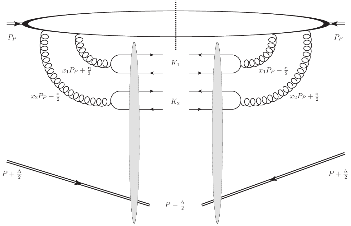
Refer to caption
Figure 3: Production of a quarkonium pair in hybrid factorization with double scattering on the projectile side

We now have all the machinery to finally compute the full differential cross section. This is straightforward but tedious, as we have to consider all possible Lorentz index structures, namely, 𝒢1,2,3,4{\cal G}_{1,2,3,4} from (3) and a1,2={g,Δ​g,δ​g}a_{1,2}=\{g,\Delta g,\delta g\} in (67). The generic result is

d​σ​(M1,M2)d​Y1​d​Y2​d2​𝚫​d2​𝑲\displaystyle\frac{d\sigma\left(M_{1},M_{2}\right)}{dY_{1}dY_{2}d^{2}\boldsymbol{\Delta}d^{2}\boldsymbol{K}} (74)
=\displaystyle= αs216​m15​m25​Nc4​(Nc2−1)2​⟨𝒪M1​(L11​J12​S1+1)⟩​⟨𝒪M2​(L12​J22​S2+1)⟩\displaystyle\frac{\alpha_{s}^{2}}{16m_{1}^{5}m_{2}^{5}N_{c}^{4}\left(N_{c}^{2}-1\right)^{2}}\left\langle\mathcal{O}_{M_{1}}\left({}^{2S_{1}+1}L_{1J_{1}}^{1}\right)\right\rangle\left\langle\mathcal{O}_{M_{2}}\left({}^{2S_{2}+1}L_{2J_{2}}^{1}\right)\right\rangle
×x1x2∫d2𝒒[δi​i′δj​j′ℱg,g(x1,x2,𝒒)−iδi​i′ϵj​j′ℱg,Δ​g(x1,x2,𝒒)+2δi​i′τj​j′,n​n′ℱg,δ​gn​n′(x1,x2,𝒒)\displaystyle\times x_{1}x_{2}\int d^{2}\boldsymbol{q}\left[\delta^{ii^{\prime}}\delta^{jj^{\prime}}\mathcal{F}_{g,g}\left(x_{1},x_{2},\boldsymbol{q}\right)-i\delta^{ii^{\prime}}\epsilon^{jj^{\prime}}\mathcal{F}_{g,\Delta g}\left(x_{1},x_{2},\boldsymbol{q}\right)+2\delta^{ii^{\prime}}\tau^{jj^{\prime},nn^{\prime}}\mathcal{F}_{g,\delta g}^{nn^{\prime}}\left(x_{1},x_{2},\boldsymbol{q}\right)\right.
−i​ϵi​i′​δj​j′​ℱΔ​g,g​(x1,x2,𝒒)−ϵi​i′​ϵj​j′​ℱΔ​g,Δ​g​(x1,x2,𝒒)−2​i​ϵi​i′​τj​j′,n​n′​ℱΔ​g,δ​gn​n′​(x1,x2,𝒒)\displaystyle-i\epsilon^{ii^{\prime}}\delta^{jj^{\prime}}\mathcal{F}_{\Delta g,g}\left(x_{1},x_{2},\boldsymbol{q}\right)-\epsilon^{ii^{\prime}}\epsilon^{jj^{\prime}}\mathcal{F}_{\Delta g,\Delta g}\left(x_{1},x_{2},\boldsymbol{q}\right)-2i\epsilon^{ii^{\prime}}\tau^{jj^{\prime},nn^{\prime}}\mathcal{F}_{\Delta g,\delta g}^{nn^{\prime}}\left(x_{1},x_{2},\boldsymbol{q}\right)
+2δj​j′τi​i′,m​m′ℱδ​g,gm​m′(x1,x2,𝒒)−2iϵj​j′τi​i′,m​m′ℱδ​g,Δ​gm​m′(x1,x2,𝒒)+4τj​j′,n​n′τi​i′,m​m′ℱδ​g,δ​gm​m′,n​n′(x1,x2,𝒒)]\displaystyle\left.+2\delta^{jj^{\prime}}\tau^{ii^{\prime},mm^{\prime}}\mathcal{F}_{\delta g,g}^{mm^{\prime}}\left(x_{1},x_{2},\boldsymbol{q}\right)-2i\epsilon^{jj^{\prime}}\tau^{ii^{\prime},mm^{\prime}}\mathcal{F}_{\delta g,\Delta g}^{mm^{\prime}}\left(x_{1},x_{2},\boldsymbol{q}\right)+4\tau^{jj^{\prime},nn^{\prime}}\tau^{ii^{\prime},mm^{\prime}}\mathcal{F}_{\delta g,\delta g}^{mm^{\prime},nn^{\prime}}\left(x_{1},x_{2},\boldsymbol{q}\right)\right]
×Π1i​i′,k​k′(M1)Π2j​j′,ℓ​ℓ′(M2)x𝒢k​ℓ(𝑲−𝒒2,𝚫)x𝒢k′ℓ′∗(𝑲+𝒒2,𝚫),\displaystyle\times\Pi_{1}^{ii^{\prime},kk^{\prime}}\left(M_{1}\right)\Pi_{2}^{jj^{\prime},\ell\ell^{\prime}}\left(M_{2}\right)x\mathcal{G}^{k\ell}\left(\boldsymbol{K}-\frac{\boldsymbol{q}}{2},\boldsymbol{\Delta}\right)x\mathcal{G}^{k^{\prime}\ell^{\prime}\ast}\left(\boldsymbol{K}+\frac{\boldsymbol{q}}{2},\boldsymbol{\Delta}\right),

where xi≡Ki+PP+,x_{i}\equiv\frac{K_{i}^{+}}{P_{P}^{+}}, 𝚫≡𝑲1+𝑲2,\boldsymbol{\Delta}\equiv\boldsymbol{K}_{1}+\boldsymbol{K}_{2}, and from now on, 𝑲≡𝑲1−𝑲22\boldsymbol{K}\equiv\frac{\boldsymbol{K}_{1}-\boldsymbol{K}_{2}}{2}. YiY_{i} the rapidity of meson MiM_{i}, and the hard subparts Π1,2\Pi_{1,2} are given by

Π1i​i′,k​k′​(η)\displaystyle\Pi_{1}^{ii^{\prime},kk^{\prime}}\left(\eta\right) =\displaystyle= δi​i′​δk​k′−δi​k′​δi′​k,\displaystyle\delta^{ii^{\prime}}\delta^{kk^{\prime}}-\delta^{ik^{\prime}}\delta^{i^{\prime}k},
Π1i​i′,k​k′​(χ0)\displaystyle\Pi_{1}^{ii^{\prime},kk^{\prime}}\left(\chi_{0}\right) =\displaystyle= 3​δi​k​δi′​k′m12,\displaystyle 3\frac{\delta^{ik}\delta^{i^{\prime}k^{\prime}}}{m_{1}^{2}}, (75)
Π1i​i′,k​k′​(χ1)\displaystyle\Pi_{1}^{ii^{\prime},kk^{\prime}}\left(\chi_{1}\right) =\displaystyle= (𝑲k+𝚫k−𝒒k2)​(𝑲k′+𝚫k′+𝒒k′2)2​m14​δi​i′,\displaystyle\frac{\left(\boldsymbol{K}^{k}+\frac{\boldsymbol{\Delta}^{k}-\boldsymbol{q}^{k}}{2}\right)\left(\boldsymbol{K}^{k^{\prime}}+\frac{\boldsymbol{\Delta}^{k^{\prime}}+\boldsymbol{q}^{k^{\prime}}}{2}\right)}{2m_{1}^{4}}\delta^{ii^{\prime}},
Π1i​i′,k​k′​(χ2)\displaystyle\Pi_{1}^{ii^{\prime},kk^{\prime}}\left(\chi_{2}\right) =\displaystyle= 2m12​[δi​i′​δk​k′−δi​k​δi′​k′+δi′​k​δi​k′+(𝑲k+𝚫k−𝒒k2)​(𝑲k′+𝚫k′+𝒒k′2)4​m12​δi​i′],\displaystyle\frac{2}{m_{1}^{2}}\left[\delta^{ii^{\prime}}\delta^{kk^{\prime}}-\delta^{ik}\delta^{i^{\prime}k^{\prime}}+\delta^{i^{\prime}k}\delta^{ik^{\prime}}+\frac{\left(\boldsymbol{K}^{k}+\frac{\boldsymbol{\Delta}^{k}-\boldsymbol{q}^{k}}{2}\right)\left(\boldsymbol{K}^{k^{\prime}}+\frac{\boldsymbol{\Delta}^{k^{\prime}}+\boldsymbol{q}^{k^{\prime}}}{2}\right)}{4m_{1}^{2}}\delta^{ii^{\prime}}\right],

for meson 1 and

Π2j​j′,ℓ​ℓ′​(η)\displaystyle\Pi_{2}^{jj^{\prime},\ell\ell^{\prime}}\left(\eta\right) =\displaystyle= δj​j′​δℓ​ℓ′−δj​ℓ′​δj′​ℓ,\displaystyle\delta^{jj^{\prime}}\delta^{\ell\ell^{\prime}}-\delta^{j\ell^{\prime}}\delta^{j^{\prime}\ell},
Π2j​j′,ℓ​ℓ′​(χ0)\displaystyle\Pi_{2}^{jj^{\prime},\ell\ell^{\prime}}\left(\chi_{0}\right) =\displaystyle= 3​δj​ℓ​δj′​ℓ′m22,\displaystyle 3\frac{\delta^{j\ell}\delta^{j^{\prime}\ell^{\prime}}}{m_{2}^{2}}, (76)
Π2j​j′,ℓ​ℓ′​(χ1)\displaystyle\Pi_{2}^{jj^{\prime},\ell\ell^{\prime}}\left(\chi_{1}\right) =\displaystyle= (𝑲ℓ−𝚫ℓ−𝒒ℓ2)​(𝑲ℓ′−𝚫ℓ′+𝒒ℓ′2)2​m24​δj​j′,\displaystyle\frac{\left(\boldsymbol{K}^{\ell}-\frac{\boldsymbol{\Delta}^{\ell}-\boldsymbol{q}^{\ell}}{2}\right)\left(\boldsymbol{K}^{\ell^{\prime}}-\frac{\boldsymbol{\Delta}^{\ell^{\prime}}+\boldsymbol{q}^{\ell^{\prime}}}{2}\right)}{2m_{2}^{4}}\delta^{jj^{\prime}},
Π2j​j′,ℓ​ℓ′​(χ2)\displaystyle\Pi_{2}^{jj^{\prime},\ell\ell^{\prime}}\left(\chi_{2}\right) =\displaystyle= 2m22​[δj​j′​δℓ​ℓ′−δj​ℓ​δj′​ℓ′+δj′​ℓ​δj​ℓ′+(𝑲ℓ−𝚫ℓ−𝒒ℓ2)​(𝑲ℓ′−𝚫ℓ′+𝒒ℓ′2)4​m22​δj​j′],\displaystyle\frac{2}{m_{2}^{2}}\left[\delta^{jj^{\prime}}\delta^{\ell\ell^{\prime}}-\delta^{j\ell}\delta^{j^{\prime}\ell^{\prime}}+\delta^{j^{\prime}\ell}\delta^{j\ell^{\prime}}+\frac{\left(\boldsymbol{K}^{\ell}-\frac{\boldsymbol{\Delta}^{\ell}-\boldsymbol{q}^{\ell}}{2}\right)\left(\boldsymbol{K}^{\ell^{\prime}}-\frac{\boldsymbol{\Delta}^{\ell^{\prime}}+\boldsymbol{q}^{\ell^{\prime}}}{2}\right)}{4m_{2}^{2}}\delta^{jj^{\prime}}\right],

for meson 2. Interestingly, the intrinsic momentum 𝒒\boldsymbol{q} of the double PDF enters the argument of the WW GTMD. Physically, 𝒒\boldsymbol{q} is conjugate to the relative distance of the two quarkonia. More precisely, it is conjugate to 𝒃1+𝒃1′2−𝒃2+𝒃2′2\frac{\boldsymbol{b}_{1}+\boldsymbol{b}^{\prime}_{1}}{2}-\frac{\boldsymbol{b}_{2}+\boldsymbol{b}^{\prime}_{2}}{2} where 𝒃1,2\boldsymbol{b}_{1,2} is as in (65) and 𝒃1,2′\boldsymbol{b}^{\prime}_{1,2} are the corresponding coordinates in the complex-conjugate amplitude.

V Explicit cross sections

In the following, we will assume that |𝑲|≫|𝒒|\left|\boldsymbol{K}\right|\gg\left|\boldsymbol{q}\right|. The dependence on 𝒒\boldsymbol{q} is then completely absorbed in the projectile Double PDF. We will thus define the integrated double PDFs

ℱa1,a2​(x1,x2)≡∫d2​𝒒​ℱa1,a2​(x1,x2,𝒒).\mathcal{F}_{a_{1},a_{2}}\left(x_{1},x_{2}\right)\equiv\int d^{2}\boldsymbol{q}\mathcal{F}_{a_{1},a_{2}}\left(x_{1},x_{2},\boldsymbol{q}\right). (77)

At this point, we can already cancel some contributions. Indeed the symmetry and tracelessness properties of the (a1=g,a2=δ​g)(a_{1}=g,a_{2}=\delta g) double PDF allows one to write it as:

ℱg,δ​gm​n​(x1,x2,𝒒)=(𝒒m​𝒒n𝒒2−δm​n2)​𝒒2MP2​ℋg,δ​g​(x1,x2,𝒒2),\mathcal{F}_{g,\delta g}^{mn}\left(x_{1},x_{2},\boldsymbol{q}\right)=\left(\frac{\boldsymbol{q}^{m}\boldsymbol{q}^{n}}{\boldsymbol{q}^{2}}-\frac{\delta^{mn}}{2}\right)\frac{\boldsymbol{q}^{2}}{M_{P}^{2}}\mathcal{H}_{g,\delta g}\left(x_{1},x_{2},\boldsymbol{q}^{2}\right), (78)

where MPM_{P} is the projectile’s mass. It is then easy to show that the integral given in 77 cancels for this integrated double PDF. Similarly, we can cancel the (a1=δ​g,a2=g)(a_{1}=\delta g,a_{2}=g) integrated double PDF.

It will also be useful to write the (a1,a2)=(δ​g,δ​g)(a_{1},a_{2})=(\delta g,\delta g) integrated double PDF as

ℱδ​g,δ​gm​m′,n​n′​(x1,x2)≡12​(δm​n​δm′​n′+δm​n′​δm′​n−δm​m′​δn​n′)​ℋδ​g,δ​g​(x1,x2).\mathcal{F}_{\delta g,\delta g}^{mm^{\prime},nn^{\prime}}\left(x_{1},x_{2}\right)\equiv\frac{1}{2}\left(\delta^{mn}\delta^{m^{\prime}n^{\prime}}+\delta^{mn^{\prime}}\delta^{m^{\prime}n}-\delta^{mm^{\prime}}\delta^{nn^{\prime}}\right)\mathcal{H}_{\delta g,\delta g}\left(x_{1},x_{2}\right). (79)

V.1 χ1​χ1\chi_{1}\chi_{1} cross section

We find that the most concise formula is obtained for the double χJ=1\chi_{J=1} production. It is given by

d​σ​(χf1​1,χf2​1)d​Y1​d​Y2​d2​𝚫​d2​𝑲\displaystyle\frac{d\sigma\left(\chi_{f_{1}1},\chi_{f_{2}1}\right)}{dY_{1}dY_{2}d^{2}\boldsymbol{\Delta}d^{2}\boldsymbol{K}} =\displaystyle= x1​x2​ℱg,g​(x1,x2)64​m19​m29​Nc4​(Nc2−1)2​αs4​⟨𝒪χf1​1​(P113)⟩​⟨𝒪χf2​1​(P113)⟩\displaystyle\frac{x_{1}x_{2}\mathcal{F}_{g,g}\left(x_{1},x_{2}\right)}{64m_{1}^{9}m_{2}^{9}N_{c}^{4}\left(N_{c}^{2}-1\right)^{2}}\alpha_{s}^{4}\left\langle\mathcal{O}_{\chi_{f_{1}1}}\left({}^{3}P_{1}^{1}\right)\right\rangle\left\langle\mathcal{O}_{\chi_{f_{2}1}}\left({}^{3}P_{1}^{1}\right)\right\rangle (80)
×|(𝑲i+𝚫i2)​(𝑲j−𝚫j2)​x​𝒢i​j​(𝑲,𝚫)|2,\displaystyle\times\left|\left(\boldsymbol{K}^{i}+\frac{\boldsymbol{\Delta}^{i}}{2}\right)\left(\boldsymbol{K}^{j}-\frac{\boldsymbol{\Delta}^{j}}{2}\right)x\mathcal{G}^{ij}\left(\boldsymbol{K},\boldsymbol{\Delta}\right)\right|^{2},

with f1,2f_{1,2} the meson flavors. To check that the right hand side has the correct dimensions, we note that dim​𝒢=−2{\rm dim}\,{\cal G}=-2, dim​ℱ=2{\rm dim}\,{\cal F}=2, and dim​⟨Oχ⟩=5{\rm dim}\,\langle O_{\chi}\rangle=5 (dim​⟨Oη⟩=3{\rm dim}\,\langle O_{\eta}\rangle=3). Explicitly, the second line of (80) reads

|(𝑲i+𝚫i2)​(𝑲j−𝚫j2)​x​𝒢i​j​(𝑲,𝚫)|2\displaystyle\left|\left(\boldsymbol{K}^{i}+\frac{\boldsymbol{\Delta}^{i}}{2}\right)\left(\boldsymbol{K}^{j}-\frac{\boldsymbol{\Delta}^{j}}{2}\right)x\mathcal{G}^{ij}\left(\boldsymbol{K},\boldsymbol{\Delta}\right)\right|^{2} (81)
=\displaystyle= 𝑲4|(1−𝚫24​𝑲2)𝒢1+(1−(𝑲⋅𝚫)22​𝑲4+𝚫24​𝑲2)𝑲22​M2𝒢2\displaystyle\boldsymbol{K}^{4}\left|\left(1-\frac{\boldsymbol{\Delta}^{2}}{4\boldsymbol{K}^{2}}\right)\mathcal{G}_{1}+\left(1-\frac{\left(\boldsymbol{K}\cdot\boldsymbol{\Delta}\right)^{2}}{2\boldsymbol{K}^{4}}+\frac{\boldsymbol{\Delta}^{2}}{4\boldsymbol{K}^{2}}\right)\frac{\boldsymbol{K}^{2}}{2M^{2}}\mathcal{G}_{2}\right.
−(𝚫22​M2−(𝑲⋅𝚫)2𝑲2​M2+𝚫48​𝑲2​M2)𝒢3−(𝚫2M2−(𝑲⋅𝚫)2𝑲2​M2)𝒢4|2\displaystyle\left.-\left(\frac{\boldsymbol{\Delta}^{2}}{2M^{2}}-\frac{\left(\boldsymbol{K}\cdot\boldsymbol{\Delta}\right)^{2}}{\boldsymbol{K}^{2}M^{2}}+\frac{\boldsymbol{\Delta}^{4}}{8\boldsymbol{K}^{2}M^{2}}\right)\mathcal{G}_{3}-\left(\frac{\boldsymbol{\Delta}^{2}}{M^{2}}-\frac{\left(\boldsymbol{K}\cdot\boldsymbol{\Delta}\right)^{2}}{\boldsymbol{K}^{2}M^{2}}\right)\mathcal{G}_{4}\right|^{2}
≈\displaystyle\approx 𝑲4​(𝒢1+𝑲22​M2​𝒢2)2,\displaystyle\boldsymbol{K}^{4}\left({\cal G}_{1}+\frac{\boldsymbol{K}^{2}}{2M^{2}}{\cal G}_{2}\right)^{2}, (82)

where the last line is obtained by assuming |𝑲|≫|𝚫||\boldsymbol{K}|\gg|\boldsymbol{\Delta}|. Remarkably, the cross section is directly proportional to the WW GTMD squared, without any convolution in momentum.

V.2 All averaged cross sections

We will now present all the full cross sections for our (M1,M2)(M_{1},M_{2}) process, for Mi∈{η,χ0,χ1,χ2}M_{i}\in\{\eta,\chi_{0},\chi_{1},\chi_{2}\}. In order to get rid of the contributions with a longitudinally polarized double PDF, we will take the average w.r.t. the angle between 𝐊\mathbf{K} and 𝚫\mathbf{\Delta}. This allows to keep only ℱg,g​(x1,x2)\mathcal{F}_{g,g}(x_{1},x_{2}) and ℋδ​g,δ​g​(x1,x2)\mathcal{H}_{\delta g,\delta g}(x_{1},x_{2}) as the non-perturbative distributions on the projectile side, since our goal is to focus rather on the non-perturbative effects on the target side.

V.2.1 (χ1​χ1)\left(\chi_{1}\chi_{1}\right)

∫02​πd​ϕ2​π​d​σ​(χf1​1,χf2​1)d​Y1​d​Y2​d2​𝑲​d​𝚫2\displaystyle\quad\quad\int_{0}^{2\pi}\frac{d\phi}{2\pi}\frac{d\sigma\left(\chi_{f_{1}1},\chi_{f_{2}1}\right)}{dY_{1}dY_{2}d^{2}\boldsymbol{K}d\boldsymbol{\Delta}^{2}}
=αs4​x2​𝑲432​m19​m29​Nc4​(Nc2−1)2​x1​x2​ℱg,g​(x1,x2)​⟨𝒪χf1​1​(P113)⟩​⟨𝒪χf2​1​(P113)⟩\displaystyle=\frac{\alpha_{s}^{4}x^{2}\boldsymbol{K}^{4}}{32m_{1}^{9}m_{2}^{9}N_{c}^{4}\left(N_{c}^{2}-1\right)^{2}}x_{1}x_{2}\mathcal{F}_{g,g}\left(x_{1},x_{2}\right)\left\langle\mathcal{O}_{\chi_{f_{1}1}}\left({}^{3}P_{1}^{1}\right)\right\rangle\left\langle\mathcal{O}_{\chi_{f_{2}1}}\left({}^{3}P_{1}^{1}\right)\right\rangle (83)
×[(𝒢1+𝑲22​M2​𝒢2)2−𝚫22​𝑲2​(𝒢1+𝑲22​M2​𝒢2)​(𝒢1+2​𝑲2M2​𝒢4)].\displaystyle\times\left[\left(\mathcal{G}_{1}+\frac{\boldsymbol{K}^{2}}{2M^{2}}\mathcal{G}_{2}\right)^{2}-\frac{\boldsymbol{\Delta}^{2}}{2\boldsymbol{K}^{2}}\left(\mathcal{G}_{1}+\frac{\boldsymbol{K}^{2}}{2M^{2}}\mathcal{G}_{2}\right)\left(\mathcal{G}_{1}+2\frac{\boldsymbol{K}^{2}}{M^{2}}\mathcal{G}_{4}\right)\right].

V.2.2 (χ1​χ0)\left(\chi_{1}\chi_{0}\right)

∫02​πd​ϕ2​π​d​σ​(χ1,χ0)d​Y1​d​Y2​d2​𝑲​d​𝚫2\displaystyle\quad\quad\int_{0}^{2\pi}\frac{d\phi}{2\pi}\frac{d\sigma\left(\chi_{1},\chi_{0}\right)}{dY_{1}dY_{2}d^{2}\boldsymbol{K}d\boldsymbol{\Delta}^{2}}
=3​αs4​x2​𝑲232​m19​m27​Nc4​(Nc2−1)2​x1​x2​ℱg,g​(x1,x2)​⟨𝒪χ1​(P113)⟩​⟨𝒪χ0​(P103)⟩\displaystyle=\frac{3\alpha_{s}^{4}x^{2}\boldsymbol{K}^{2}}{32m_{1}^{9}m_{2}^{7}N_{c}^{4}\left(N_{c}^{2}-1\right)^{2}}x_{1}x_{2}\mathcal{F}_{g,g}\left(x_{1},x_{2}\right)\left\langle\mathcal{O}_{\chi_{1}}\left({}^{3}P_{1}^{1}\right)\right\rangle\left\langle\mathcal{O}_{\chi_{0}}\left({}^{3}P_{0}^{1}\right)\right\rangle
×[(𝒢1+𝑲22​M2​𝒢2)2+𝚫24​𝑲2​(𝒢12+𝑲44​M4​(𝒢22−8​𝒢2​𝒢4+8​𝒢42))]\displaystyle\times\left[\left(\mathcal{G}_{1}+\frac{\boldsymbol{K}^{2}}{2M^{2}}\mathcal{G}_{2}\right)^{2}+\frac{\boldsymbol{\Delta}^{2}}{4\boldsymbol{K}^{2}}\left(\mathcal{G}_{1}^{2}+\frac{\boldsymbol{K}^{4}}{4M^{4}}\left(\mathcal{G}_{2}^{2}-8\mathcal{G}_{2}\mathcal{G}_{4}+8\mathcal{G}_{4}^{2}\right)\right)\right] (84)

V.2.3 (χ1​χ2)\left(\chi_{1}\chi_{2}\right)

∫02​πd​ϕ2​π​d​σ​(χ1,χ2)d​Y1​d​Y2​d2​𝑲​d​𝚫2\displaystyle\quad\quad\int_{0}^{2\pi}\frac{d\phi}{2\pi}\frac{d\sigma\left(\chi_{1},\chi_{2}\right)}{dY_{1}dY_{2}d^{2}\boldsymbol{K}d\boldsymbol{\Delta}^{2}}
=αs4​𝑲2​x28​m17​m27​Nc4​(Nc2−1)2​⟨𝒪χ1​(P113)⟩​⟨𝒪χ2​(P123)⟩\displaystyle=\frac{\alpha_{s}^{4}\boldsymbol{K}^{2}x^{2}}{8m_{1}^{7}m_{2}^{7}N_{c}^{4}\left(N_{c}^{2}-1\right)^{2}}\left\langle\mathcal{O}_{\chi_{1}}\left({}^{3}P_{1}^{1}\right)\right\rangle\left\langle\mathcal{O}_{\chi_{2}}\left({}^{3}P_{2}^{1}\right)\right\rangle (85)
×x1x2ℱg,g(x1,x2){(1+𝑲24​m22)(𝒢1+𝑲22​M2𝒢2)2\displaystyle\times x_{1}x_{2}\mathcal{F}_{g,g}\left(x_{1},x_{2}\right)\left\{\left(1+\frac{\boldsymbol{K}^{2}}{4m_{2}^{2}}\right)\left(\mathcal{G}_{1}+\frac{\boldsymbol{K}^{2}}{2M^{2}}\mathcal{G}_{2}\right)^{2}\right.
+𝚫24​𝑲2[(1+𝑲2m22)𝒢12+3​𝑲44​m22​M2𝒢1𝒢2+𝑲44​M4(1+𝑲22​m22)𝒢22−2𝑲4M4(𝒢2−𝒢4)𝒢4]}\displaystyle\left.+\frac{\boldsymbol{\Delta}^{2}}{4\boldsymbol{K}^{2}}\left[\left(1+\frac{\boldsymbol{K}^{2}}{m_{2}^{2}}\right)\mathcal{G}_{1}^{2}+\frac{3\boldsymbol{K}^{4}}{4m_{2}^{2}M^{2}}\mathcal{G}_{1}\mathcal{G}_{2}+\frac{\boldsymbol{K}^{4}}{4M^{4}}\left(1+\frac{\boldsymbol{K}^{2}}{2m_{2}^{2}}\right)\mathcal{G}_{2}^{2}-2\frac{\boldsymbol{K}^{4}}{M^{4}}\left(\mathcal{G}_{2}-\mathcal{G}_{4}\right)\mathcal{G}_{4}\right]\right\}

V.2.4 (χ1​η)\left(\chi_{1}\eta\right)

12​π​∫02​πd​ϕ​d​σ​(χ1,η)d​Y1​d​Y2​d​𝚫2​d2​𝑲\displaystyle\quad\quad\frac{1}{2\pi}\int_{0}^{2\pi}d\phi\frac{d\sigma\left(\chi_{1},\eta\right)}{dY_{1}dY_{2}d\boldsymbol{\Delta}^{2}d^{2}\boldsymbol{K}} (86)
=\displaystyle= αs4​x2​𝑲232​m17​m25​Nc4​(Nc2−1)2​x1​x2​ℱg,g​(x1,x2)​⟨𝒪χ1​(P113)⟩​⟨𝒪η​(S101)⟩\displaystyle\frac{\alpha_{s}^{4}x^{2}\boldsymbol{K}^{2}}{32m_{1}^{7}m_{2}^{5}N_{c}^{4}\left(N_{c}^{2}-1\right)^{2}}x_{1}x_{2}\mathcal{F}_{g,g}\left(x_{1},x_{2}\right)\left\langle\mathcal{O}_{\chi_{1}}\left({}^{3}P_{1}^{1}\right)\right\rangle\left\langle\mathcal{O}_{\eta}\left({}^{1}S_{0}^{1}\right)\right\rangle
×[(𝒢1+𝑲22​M2​𝒢2)2+𝚫24​𝑲2​(𝒢12+𝑲44​M4​(𝒢22−8​𝒢2​𝒢4+8​𝒢42))]\displaystyle\times\left[\left(\mathcal{G}_{1}+\frac{\boldsymbol{K}^{2}}{2M^{2}}\mathcal{G}_{2}\right)^{2}+\frac{\boldsymbol{\Delta}^{2}}{4\boldsymbol{K}^{2}}\left(\mathcal{G}_{1}^{2}+\frac{\boldsymbol{K}^{4}}{4M^{4}}\left(\mathcal{G}_{2}^{2}-8\mathcal{G}_{2}\mathcal{G}_{4}+8\mathcal{G}_{4}^{2}\right)\right)\right]

V.2.5 (χ0​χ0)\left(\chi_{0}\chi_{0}\right)

∫02​πd​ϕ2​π​d​σ​(χf1​0,χf2​0)d​Y1​d​Y2​d2​𝑲​d​𝚫2\displaystyle\quad\quad\int_{0}^{2\pi}\frac{d\phi}{2\pi}\frac{d\sigma\left(\chi_{f_{1}0},\chi_{f_{2}0}\right)}{dY_{1}dY_{2}d^{2}\boldsymbol{K}d\boldsymbol{\Delta}^{2}}
=9​αs4​x216​m17​m27​Nc4​(Nc2−1)2​⟨𝒪χf1​0​(P103)⟩​⟨𝒪χf2​0​(P103)⟩\displaystyle=\frac{9\alpha_{s}^{4}x^{2}}{16m_{1}^{7}m_{2}^{7}N_{c}^{4}\left(N_{c}^{2}-1\right)^{2}}\left\langle\mathcal{O}_{\chi_{f_{1}0}}\left({}^{3}P_{0}^{1}\right)\right\rangle\left\langle\mathcal{O}_{\chi_{f_{2}0}}\left({}^{3}P_{0}^{1}\right)\right\rangle
×{x1x2ℱg,g(x1,x2)(𝒢12+𝑲44​M4𝒢22+𝑲2​𝚫22​M4𝒢42)\displaystyle\times\left\{x_{1}x_{2}\mathcal{F}_{g,g}\left(x_{1},x_{2}\right)\left(\mathcal{G}_{1}^{2}+\frac{\boldsymbol{K}^{4}}{4M^{4}}\mathcal{G}_{2}^{2}+\frac{\boldsymbol{K}^{2}\boldsymbol{\Delta}^{2}}{2M^{4}}\mathcal{G}_{4}^{2}\right)\right. (87)
+4x1x2ℋδ​g,δ​g(x1,x2)[𝒢12−2𝚫2M2(𝒢1𝒢3−𝑲24​M2𝒢42)]}\displaystyle\left.+4x_{1}x_{2}\mathcal{H}_{\delta g,\delta g}\left(x_{1},x_{2}\right)\left[\mathcal{G}_{1}^{2}-2\frac{\boldsymbol{\Delta}^{2}}{M^{2}}\left(\mathcal{G}_{1}\mathcal{G}_{3}-\frac{\boldsymbol{K}^{2}}{4M^{2}}\mathcal{G}_{4}^{2}\right)\right]\right\}

V.2.6 (χ0​χ2)\left(\chi_{0}\chi_{2}\right)

∫02​πd​ϕ2​π​d​σ​(χ0,χ2)d​Y1​d​Y2​d2​𝑲​d​𝚫2\displaystyle\quad\quad\int_{0}^{2\pi}\frac{d\phi}{2\pi}\frac{d\sigma\left(\chi_{0},\chi_{2}\right)}{dY_{1}dY_{2}d^{2}\boldsymbol{K}d\boldsymbol{\Delta}^{2}}
=3​αs4​x216​m17​m27​Nc4​(Nc2−1)2​x1​x2​ℱg,g​(x1,x2)​⟨𝒪χ0​(P103)⟩​⟨𝒪χ2​(P123)⟩\displaystyle=\frac{3\alpha_{s}^{4}x^{2}}{16m_{1}^{7}m_{2}^{7}N_{c}^{4}\left(N_{c}^{2}-1\right)^{2}}x_{1}x_{2}\mathcal{F}_{g,g}\left(x_{1},x_{2}\right)\left\langle\mathcal{O}_{\chi_{0}}\left({}^{3}P_{0}^{1}\right)\right\rangle\left\langle\mathcal{O}_{\chi_{2}}\left({}^{3}P_{2}^{1}\right)\right\rangle
×[4𝒢12+𝑲4M4𝒢22+𝑲22​m22(𝒢1+𝑲22​M2𝒢2)2\displaystyle\times\left[4\mathcal{G}_{1}^{2}+\frac{\boldsymbol{K}^{4}}{M^{4}}\mathcal{G}_{2}^{2}+\frac{\boldsymbol{K}^{2}}{2m_{2}^{2}}\left(\mathcal{G}_{1}+\frac{\boldsymbol{K}^{2}}{2M^{2}}\mathcal{G}_{2}\right)^{2}\right. (88)
+𝚫28​M2(M2m22𝒢12+16𝑲2M2𝒢42+𝑲44​m22​M2(𝒢22+8𝒢2𝒢4+8𝒢42))]\displaystyle\left.+\frac{\boldsymbol{\Delta}^{2}}{8M^{2}}\left(\frac{M^{2}}{m_{2}^{2}}\mathcal{G}_{1}^{2}+16\frac{\boldsymbol{K}^{2}}{M^{2}}\mathcal{G}_{4}^{2}+\frac{\boldsymbol{K}^{4}}{4m_{2}^{2}M^{2}}\left(\mathcal{G}_{2}^{2}+8\mathcal{G}_{2}\mathcal{G}_{4}+8\mathcal{G}_{4}^{2}\right)\right)\right]

V.2.7 (χ0​η)\left(\chi_{0}\eta\right)

∫02​πd​ϕ2​π​d​σ​(χ0,η)d​Y1​d​Y2​d2​𝑲​d​𝚫2\displaystyle\quad\quad\int_{0}^{2\pi}\frac{d\phi}{2\pi}\frac{d\sigma\left(\chi_{0},\eta\right)}{dY_{1}dY_{2}d^{2}\boldsymbol{K}d\boldsymbol{\Delta}^{2}}
=3​αs4​x216​m17​m25​Nc4​(Nc2−1)2​⟨𝒪χ0​(P103)⟩​⟨𝒪η​(S101)⟩\displaystyle=\frac{3\alpha_{s}^{4}x^{2}}{16m_{1}^{7}m_{2}^{5}N_{c}^{4}\left(N_{c}^{2}-1\right)^{2}}\left\langle\mathcal{O}_{\chi_{0}}\left({}^{3}P_{0}^{1}\right)\right\rangle\left\langle\mathcal{O}_{\eta}\left({}^{1}S_{0}^{1}\right)\right\rangle
{x1x2ℱg,g(x1,x2)(𝒢12+𝑲44​M4𝒢22+𝑲2​𝚫22​M4𝒢42)\displaystyle\left\{x_{1}x_{2}\mathcal{F}_{g,g}\left(x_{1},x_{2}\right)\left(\mathcal{G}_{1}^{2}+\frac{\boldsymbol{K}^{4}}{4M^{4}}\mathcal{G}_{2}^{2}+\frac{\boldsymbol{K}^{2}\boldsymbol{\Delta}^{2}}{2M^{4}}\mathcal{G}_{4}^{2}\right)\right. (89)
−4x1x2ℋδ​g,δ​g(x1,x2)[𝒢12−2𝚫2M2(𝒢1𝒢3−𝑲24​M2𝒢42)]}\displaystyle\left.-4x_{1}x_{2}\mathcal{H}_{\delta g,\delta g}\left(x_{1},x_{2}\right)\left[\mathcal{G}_{1}^{2}-2\frac{\boldsymbol{\Delta}^{2}}{M^{2}}\left(\mathcal{G}_{1}\mathcal{G}_{3}-\frac{\boldsymbol{K}^{2}}{4M^{2}}\mathcal{G}_{4}^{2}\right)\right]\right\}

V.2.8 (χ2​χ2)\left(\chi_{2}\chi_{2}\right)

∫02​πd​ϕ2​π​d​σ​(χf1​2,χf2​2)d​Y1​d​Y2​d2​𝑲​d​𝚫2\displaystyle\quad\quad\int_{0}^{2\pi}\frac{d\phi}{2\pi}\frac{d\sigma\left(\chi_{f_{1}2},\chi_{f_{2}2}\right)}{dY_{1}dY_{2}d^{2}\boldsymbol{K}d\boldsymbol{\Delta}^{2}}
=αs4​x28​m17​m27​Nc4​(Nc2−1)2​x1​x2​ℱg,g​(x1,x2)​⟨𝒪χf1​2​(P123)⟩​⟨𝒪χf2​2​(P123)⟩\displaystyle=\frac{\alpha_{s}^{4}x^{2}}{8m_{1}^{7}m_{2}^{7}N_{c}^{4}\left(N_{c}^{2}-1\right)^{2}}x_{1}x_{2}\mathcal{F}_{g,g}\left(x_{1},x_{2}\right)\left\langle\mathcal{O}_{\chi_{f_{1}2}}\left({}^{3}P_{2}^{1}\right)\right\rangle\left\langle\mathcal{O}_{\chi_{f_{2}2}}\left({}^{3}P_{2}^{1}\right)\right\rangle
×{8(𝒢12+𝑲44​M4𝒢22)+(𝑲2m12+𝑲2m22+𝑲44​m12​m22)(𝒢1+𝑲22​M2𝒢2)2\displaystyle\times\left\{8\left(\mathcal{G}_{1}^{2}+\frac{\boldsymbol{K}^{4}}{4M^{4}}\mathcal{G}_{2}^{2}\right)+\left(\frac{\boldsymbol{K}^{2}}{m_{1}^{2}}+\frac{\boldsymbol{K}^{2}}{m_{2}^{2}}+\frac{\boldsymbol{K}^{4}}{4m_{1}^{2}m_{2}^{2}}\right)\left(\mathcal{G}_{1}+\frac{\boldsymbol{K}^{2}}{2M^{2}}\mathcal{G}_{2}\right)^{2}\right.
+𝚫232​m12​m22​[8​𝒢12​(𝑲2+m12+m22)+6​𝑲2​𝑲2M2​𝒢1​𝒢2+𝑲4M4​(𝑲2+2​m12+2​m22)​𝒢22]\displaystyle+\frac{\boldsymbol{\Delta}^{2}}{32m_{1}^{2}m_{2}^{2}}\left[8\mathcal{G}_{1}^{2}\left(\boldsymbol{K}^{2}+m_{1}^{2}+m_{2}^{2}\right)+6\boldsymbol{K}^{2}\frac{\boldsymbol{K}^{2}}{M^{2}}\mathcal{G}_{1}\mathcal{G}_{2}+\frac{\boldsymbol{K}^{4}}{M^{4}}\left(\boldsymbol{K}^{2}+2m_{1}^{2}+2m_{2}^{2}\right)\mathcal{G}_{2}^{2}\right] (90)
+𝚫22​m12​m22𝑲2M2[(m12−m22)𝑲2M2𝒢2𝒢4+(𝑲2​m12M2+𝑲2​m22M2+8m12​m22M2)𝒢42]}\displaystyle\left.+\frac{\boldsymbol{\Delta}^{2}}{2m_{1}^{2}m_{2}^{2}}\frac{\boldsymbol{K}^{2}}{M^{2}}\left[\left(m_{1}^{2}-m_{2}^{2}\right)\frac{\boldsymbol{K}^{2}}{M^{2}}\mathcal{G}_{2}\mathcal{G}_{4}+\left(\frac{\boldsymbol{K}^{2}m_{1}^{2}}{M^{2}}+\frac{\boldsymbol{K}^{2}m_{2}^{2}}{M^{2}}+8\frac{m_{1}^{2}m_{2}^{2}}{M^{2}}\right)\mathcal{G}_{4}^{2}\right]\right\}

V.2.9 (χ2​η)\left(\chi_{2}\eta\right)

∫02​πd​ϕ2​π​d​σ​(χ2,η)d​Y1​d​Y2​d2​𝑲​d​𝚫2\displaystyle\quad\quad\int_{0}^{2\pi}\frac{d\phi}{2\pi}\frac{d\sigma\left(\chi_{2},\eta\right)}{dY_{1}dY_{2}d^{2}\boldsymbol{K}d\boldsymbol{\Delta}^{2}}
=αs4​x216​m17​m25​Nc4​(Nc2−1)2​⟨𝒪χ2​(P123)⟩​⟨𝒪η​(S101)⟩\displaystyle=\frac{\alpha_{s}^{4}x^{2}}{16m_{1}^{7}m_{2}^{5}N_{c}^{4}\left(N_{c}^{2}-1\right)^{2}}\left\langle\mathcal{O}_{\chi_{2}}\left({}^{3}P_{2}^{1}\right)\right\rangle\left\langle\mathcal{O}_{\eta}\left({}^{1}S_{0}^{1}\right)\right\rangle (91)
×x1x2ℱg,g(x1,x2)[4(𝒢12+𝑲44​M4𝒢22)+𝑲22​m12(𝒢1+𝑲22​M2𝒢2)2\displaystyle\times x_{1}x_{2}\mathcal{F}_{g,g}\left(x_{1},x_{2}\right)\left[4\left(\mathcal{G}_{1}^{2}+\frac{\boldsymbol{K}^{4}}{4M^{4}}\mathcal{G}_{2}^{2}\right)+\frac{\boldsymbol{K}^{2}}{2m_{1}^{2}}\left(\mathcal{G}_{1}+\frac{\boldsymbol{K}^{2}}{2M^{2}}\mathcal{G}_{2}\right)^{2}\right.
+𝚫28​m12(𝒢12+𝑲44​M4(𝒢22−8𝒢2𝒢4+8𝒢42)+16𝑲2M2m12M2𝒢42)]\displaystyle\left.+\frac{\boldsymbol{\Delta}^{2}}{8m_{1}^{2}}\left(\mathcal{G}_{1}^{2}+\frac{\boldsymbol{K}^{4}}{4M^{4}}\left(\mathcal{G}_{2}^{2}-8\mathcal{G}_{2}\mathcal{G}_{4}+8\mathcal{G}_{4}^{2}\right)+16\frac{\boldsymbol{K}^{2}}{M^{2}}\frac{m_{1}^{2}}{M^{2}}\mathcal{G}_{4}^{2}\right)\right]

V.2.10 (η​η)\left(\eta\eta\right)

∫02​πd​ϕ2​π​d​σ​(ηf1,ηf2)d​Y1​d​Y2​d2​𝑲​d​𝚫2\displaystyle\quad\quad\int_{0}^{2\pi}\frac{d\phi}{2\pi}\frac{d\sigma\left(\eta_{f_{1}},\eta_{f_{2}}\right)}{dY_{1}dY_{2}d^{2}\boldsymbol{K}d\boldsymbol{\Delta}^{2}}
=αs4​x216​m15​m25​Nc4​(Nc2−1)2​⟨𝒪ηf1​(S101)⟩​⟨𝒪ηf2​(S101)⟩\displaystyle=\frac{\alpha_{s}^{4}x^{2}}{16m_{1}^{5}m_{2}^{5}N_{c}^{4}\left(N_{c}^{2}-1\right)^{2}}\left\langle\mathcal{O}_{\eta_{f_{1}}}\left({}^{1}S_{0}^{1}\right)\right\rangle\left\langle\mathcal{O}_{\eta_{f_{2}}}\left({}^{1}S_{0}^{1}\right)\right\rangle
×{x1x2ℱg,g(x1,x2)(𝒢12+𝑲44​M4𝒢22+𝑲2​𝚫22​M4𝒢42)\displaystyle\times\left\{x_{1}x_{2}\mathcal{F}_{g,g}\left(x_{1},x_{2}\right)\left(\mathcal{G}_{1}^{2}+\frac{\boldsymbol{K}^{4}}{4M^{4}}\mathcal{G}_{2}^{2}+\frac{\boldsymbol{K}^{2}\boldsymbol{\Delta}^{2}}{2M^{4}}\mathcal{G}_{4}^{2}\right)\right. (92)
+4x1x2ℋδ​g,δ​g(x1,x2)[𝒢12−2𝚫2M2(𝒢1𝒢3−𝑲24​M2𝒢42)]}.\displaystyle\left.+4x_{1}x_{2}\mathcal{H}_{\delta g,\delta g}\left(x_{1},x_{2}\right)\left[\mathcal{G}_{1}^{2}-2\frac{\boldsymbol{\Delta}^{2}}{M^{2}}\left(\mathcal{G}_{1}\mathcal{G}_{3}-\frac{\boldsymbol{K}^{2}}{4M^{2}}\mathcal{G}_{4}^{2}\right)\right]\right\}.

VI Conclusions

In summary, in this paper we derive the diffractive double quarkonia production in p​ppp and p​ApA collisions to probe the WW gluon GTMDs. In particular, we applied the double parton scattering mechanism from the projectile, where the two gluons scatter off the nucleon/nucleus target diffractively to produce the final state two quarkonium states. The amplitudes are found to be sensitive to the WW gluon GTMDs.

More importantly, we found that the differential cross sections can be much simplified if we integrate out the transverse momenta of the gluons from the projectile. The explicit expressions show that the cross sections can be written as squared of the WW gluon GTMDs from the target.

Our result is a first example of direct access to the WW gluon GTMDs in hard diffractive processes. Experimentally, this process may be a challenge to measure. We hope that our derivations will stimulate further theoretical developments to explore the physics of GTMD and possibility to measure them in experiments.

Acknowledgements.
This work is supported by the National Science Center, Poland, grant No. 2015/17/B/ST2/01838. It is also partially supported by the Natural Science Foundation of China (NSFC) under Grant Nos. 11575070 and by the U.S. Department of Energy, Office of Science, Office of Nuclear Physics, under contract number DE-AC02-05CH11231.

Appendix A Gluon to S01{}^{1}S_{0} and PJ3{}^{3}P_{J} waves transition in the hybrid formalism

For completeness, here we write down the cross section for the single-inclusive quarkonium production g​p→M​Xgp\to MX for S01{}^{1}S_{0} and PJ3{}^{3}P_{J} waves. Squaring (63) and using the projectors (68)–(72), we find

d​σg​(M)d​K+​d2​𝑲\displaystyle\frac{d\sigma_{g}(M)}{dK^{+}d^{2}\boldsymbol{K}} =\displaystyle= αs2​m5​Nc​(Nc2−1)​δ​(K+−k+)​∫d2​𝒃​d2​𝒃′(2​π)2​ei​𝑲⋅(𝒃′−𝒃)\displaystyle\frac{\alpha_{s}}{2m^{5}N_{c}\left(N_{c}^{2}-1\right)}\delta(K^{+}-k^{+})\int\frac{d^{2}\boldsymbol{b}d^{2}\boldsymbol{b}^{\prime}}{\left(2\pi\right)^{2}}e^{i\boldsymbol{K}\cdot(\boldsymbol{b}^{\prime}-\boldsymbol{b})}
×⟨1NcTr[U𝒃†(∂iU𝒃)U𝒃′†(∂jU𝒃′)]⟩φi​j(2​S+1LJ)⟨𝒪M(2​S+1LJ1)⟩12,\displaystyle\times\left\langle\frac{1}{N_{c}}\mathrm{Tr}\left[U_{\boldsymbol{b}}^{\dagger}(\partial_{i}U_{\boldsymbol{b}})U_{\boldsymbol{b}^{\prime}}^{\dagger}(\partial_{j}U_{\boldsymbol{b}^{\prime}})\right]\right\rangle\varphi^{ij}(^{2S+1}L_{J})\left\langle{\cal O}_{M}(^{2S+1}L_{J}^{1})\right\rangle^{\frac{1}{2}},

where

φi​j(1S0)\displaystyle\varphi^{ij}(^{1}S_{0}) =\displaystyle= δi​j,\displaystyle\delta^{ij},
φi​j(3P0)\displaystyle\varphi^{ij}(^{3}P_{0}) =\displaystyle= 3​δi​jm2,\displaystyle\frac{3\delta^{ij}}{m^{2}}, (93)
φi​j(3P1)\displaystyle\varphi^{ij}(^{3}P_{1}) =\displaystyle= Ki​Kjm4,\displaystyle\frac{K^{i}K^{j}}{m^{4}},
φi​j(3P2)\displaystyle\varphi^{ij}(^{3}P_{2}) =\displaystyle= 4m2​(δi​j+Ki​Kj4​m2),\displaystyle\frac{4}{m^{2}}\left(\delta^{ij}+\frac{K^{i}K^{j}}{4m^{2}}\right),

and the brackets denote the forward matrix element ⟨P|…|P⟩⟨P|P⟩\frac{\langle P|...|P\rangle}{\langle P|P\rangle}, or equivalently the CGC averaging.
Taking the case where M=J/ψM=J/\psi and taking the small-dipole limit in the collinear limit of results described in [33] shows full compatibility of the present results with previous calculations.

References

  • [1] X. d. Ji, Phys. Rev. Lett. 91, 062001 (2003) [hep-ph/0304037].
  • [2] A. V. Belitsky, X. d. Ji and F. Yuan, Phys. Rev. D 69, 074014 (2004) [hep-ph/0307383].
  • [3] C. Lorce and B. Pasquini, Phys. Rev. D 84, 014015 (2011) doi:10.1103/PhysRevD.84.014015 [arXiv:1106.0139 [hep-ph]].
  • [4] S. Meissner, A. Metz and M. Schlegel, JHEP 0908, 056 (2009) [arXiv:0906.5323 [hep-ph]].
  • [5] C. Lorce and B. Pasquini, JHEP 1309, 138 (2013) [arXiv:1307.4497 [hep-ph]].
  • [6] M. G. Echevarria, A. Idilbi, K. Kanazawa, C. Lorcé, A. Metz, B. Pasquini and M. Schlegel, Phys. Lett. B 759, 336 (2016) [arXiv:1602.06953 [hep-ph]].
  • [7] P. J. Mulders and J. Rodrigues, Phys. Rev. D 63, 094021 (2001) [arXiv:hep-ph/0009343].
  • [8] C. J. Bomhof, P. J. Mulders and F. Pijlman, Eur. Phys. J. C 47, 147 (2006).
  • [9] B. W. Xiao and F. Yuan, Phys. Rev. Lett. 105, 062001 (2010) [arXiv:1003.0482 [hep-ph]].
  • [10] F. Dominguez, B. W. Xiao and F. Yuan, Phys. Rev. Lett. 106, 022301 (2011) [arXiv:1009.2141 [hep-ph]].
  • [11] F. Dominguez, C. Marquet, B. W. Xiao and F. Yuan, Phys. Rev. D 83, 105005 (2011) [arXiv:1101.0715 [hep-ph]].
  • [12] Y. Hatta, B. W. Xiao and F. Yuan, Phys. Rev. Lett. 116, no. 20, 202301 (2016) [arXiv:1601.01585 [hep-ph]].
  • [13] D. Boer et al., arXiv:1108.1713 [nucl-th].
  • [14] J. L. Abelleira Fernandez et al. [LHeC Study Group Collaboration], J. Phys. G 39, 075001 (2012).
  • [15] A. Accardi et al., Eur. Phys. J. A 52, no. 9, 268 (2016), arXiv:1212.1701 [nucl-ex].
  • [16] E. C. Aschenauer et al., arXiv:1708.01527 [nucl-ex].
  • [17] R. Boussarie, A. V. Grabovsky, L. Szymanowski and S. Wallon, JHEP 1611, 149 (2016) [arXiv:1606.00419 [hep-ph]].
  • [18] Y. Hagiwara, Y. Hatta and T. Ueda, Phys. Rev. D 94, no. 9, 094036 (2016) [arXiv:1609.05773 [hep-ph]].
  • [19] J. Zhou, Phys. Rev. D 94, no. 11, 114017 (2016) [arXiv:1611.02397 [hep-ph]].
  • [20] X. Ji, F. Yuan and Y. Zhao, Phys. Rev. Lett. 118, no. 19, 192004 (2017) [arXiv:1612.02438 [hep-ph]].
  • [21] Y. Hatta, Y. Nakagawa, F. Yuan, Y. Zhao and B. Xiao, Phys. Rev. D 95, no. 11, 114032 (2017) [arXiv:1612.02445 [hep-ph]].
  • [22] Y. Hagiwara, Y. Hatta, B. W. Xiao and F. Yuan, Phys. Lett. B 771, 374 (2017) [arXiv:1701.04254 [hep-ph]].
  • [23] S. Bhattacharya, A. Metz and J. Zhou, Phys. Lett. B 771, 396 (2017) [arXiv:1702.04387 [hep-ph]].
  • [24] Y. Hatta, B. W. Xiao and F. Yuan, Phys. Rev. D 95, no. 11, 114026 (2017) [arXiv:1703.02085 [hep-ph]].
  • [25] Y. Hagiwara, Y. Hatta, R. Pasechnik, M. Tasevsky and O. Teryaev, Phys. Rev. D 96, no. 3, 034009 (2017) [arXiv:1706.01765 [hep-ph]].
  • [26] J. More, A. Mukherjee and S. Nair, Eur. Phys. J. C 78, no. 5, 389 (2018) doi:10.1140/epjc/s10052-018-5858-1 [arXiv:1709.00943 [hep-ph]].
  • [27] A. Rajan, M. Engelhardt and S. Liuti, arXiv:1709.05770 [hep-ph].
  • [28] Y. Hagiwara, Y. Hatta, B. W. Xiao and F. Yuan, arXiv:1801.00087 [hep-ph].
  • [29] Y. Hatta, Phys. Lett. B 708, 186 (2012) doi:10.1016/j.physletb.2012.01.024 [arXiv:1111.3547 [hep-ph]].
  • [30] Y. Zhao, K. F. Liu and Y. Yang, Phys. Rev. D 93, no. 5, 054006 (2016) [arXiv:1506.08832 [hep-ph]].
  • [31] S. Bhattacharya, A. Metz, V. K. Ojha, J. Y. Tsai and J. Zhou, arXiv:1802.10550 [hep-ph].
  • [32] D. Boer, T. Van Daal, P. J. Mulders and E. Petreska, arXiv:1805.05219 [hep-ph].
  • [33] Z. B. Kang, Y. Q. Ma and R. Venugopalan, JHEP 1401, 056 (2014) doi:10.1007/JHEP01(2014)056 [arXiv:1309.7337 [hep-ph]].
  • [34] J. W. Qiu, P. Sun, B. W. Xiao and F. Yuan, Phys. Rev. D 89, no. 3, 034007 (2014) [arXiv:1310.2230 [hep-ph]].
  • [35] L. D. McLerran and R. Venugopalan, Phys. Rev. D 50, 2225 (1994) doi:10.1103/PhysRevD.50.2225 [hep-ph/9402335].
  • [36] I. Balitsky, Nucl. Phys. B 463, 99 (1996) doi:10.1016/0550-3213(95)00638-9 [hep-ph/9509348].
  • [37] R. Boussarie, A. V. Grabovsky, L. Szymanowski and S. Wallon, JHEP 1409, 026 (2014) [arXiv:1405.7676 [hep-ph]].
  • [38] A. Metz and J. Zhou, Phys. Rev. D 84, 051503 (2011) doi:10.1103/PhysRevD.84.051503 [arXiv:1105.1991 [hep-ph]].
  • [39] F. Dominguez, J. W. Qiu, B. W. Xiao and F. Yuan, Phys. Rev. D 85, 045003 (2012) [arXiv:1109.6293 [hep-ph]].
  • [40] P. Sun, B. W. Xiao and F. Yuan, Phys. Rev. D 84, 094005 (2011) [arXiv:1109.1354 [hep-ph]].
  • [41] D. Boer, W. J. den Dunnen, C. Pisano, M. Schlegel and W. Vogelsang, Phys. Rev. Lett. 108, 032002 (2012).
  • [42] A. Dumitru, T. Lappi and V. Skokov, Phys. Rev. Lett. 115, no. 25, 252301 (2015) [arXiv:1508.04438 [hep-ph]].
  • [43] G. T. Bodwin, E. Braaten and G. P. Lepage, Phys. Rev. D51, 1125 (1995); Erratum, Phys. Rev. D 55, 5853(E) (1997) [arXiv:9407339 [hep-ph]].
  • [44] H. S. Shao, Y. Q. Ma, K. Wang and K. T. Chao, Phys. Rev. Lett. 112, no. 18, 182003 (2014) doi:10.1103/PhysRevLett.112.182003 [arXiv:1402.2913 [hep-ph]].
  • [45] H. Han, Y. Q. Ma, C. Meng, H. S. Shao and K. T. Chao, Phys. Rev. Lett. 114, no. 9, 092005 (2015) doi:10.1103/PhysRevLett.114.092005 [arXiv:1411.7350 [hep-ph]].
  • [46] M. Butenschoen, Z. G. He and B. A. Kniehl, Phys. Rev. Lett. 114, no. 9, 092004 (2015) doi:10.1103/PhysRevLett.114.092004 [arXiv:1411.5287 [hep-ph]].
  • [47] P. Hagler, R. Kirschner, A. Schafer, L. Szymanowski and O. V. Teryaev, Phys. Rev. Lett. 86, 1446 (2001) doi:10.1103/PhysRevLett.86.1446 [hep-ph/0004263].
  • [48] S. P. Baranov, A. V. Lipatov and N. P. Zotov, Phys. Rev. D 93, no. 9, 094012 (2016) doi:10.1103/PhysRevD.93.094012 [arXiv:1510.02411 [hep-ph]].
  • [49] M. G. A. Buffing, M. Diehl and T. Kasemets, JHEP 1801, 044 (2018) doi:10.1007/JHEP01(2018)044 [arXiv:1708.03528 [hep-ph]].