∎
Tracking Mobile Intruders in an Art Gallery: Guard Deployment Strategies, Fundamental Limitations, and Performance Guarantees
Abstract
This paper addresses the problem of tracking mobile intruders in a polygonal environment. We assume that a team of diagonal guards is deployed inside the polygon to provide mobile coverage. First, we formulate the problem of tracking a mobile intruder inside a polygonal environment as a multi-robot task allocation (MRTA) problem. Leveraging on guard deployment strategies in art gallery problems for mobile coverage, we show that the problem of finding the minimum speed of guards to persistently track a single mobile intruder is NP-hard. Next, for a given maximum speed of the intruder and the guards, we propose a technique to partition a polygon, and compute a feasible allocation of guards to the partitions. We prove the correctness of the proposed algorithm, and show its completeness for a specific class of inputs. We classify the guards based on the structural properties of the partitions allocated to them. Based on the classification, we propose motion strategy for the guards to track the mobile intruder when it is located in the partition allocated to the guard. Finally, we extend the proposed technique to address guard deployment and allocation strategies for non-simple polygons and multiple intruders.
Keywords:
Target tracking, Mobile coverage, Art gallery, Multi-robot task allocation, Sliding cameras1 Introduction
Security is an important concern in infrastructure systems. For decades, autonomous mobile robots have been utilized as surveillance [1][2] and crime-fighting agents for barrier assessments [3][4], intruder detection [5][6], building virtual terrains or maps [7][8], neutralizing explosives [9][10], and recognizing abnormal human behaviors [11][12]. Such robots have been designed with the ability to counter threats, limit risks to personnel, and reduce manpower requirements in hazardous environments [13][14][3]. Deployment of these surveillance platforms in teams has given rise to challenging problems in collaborative sensing and decision-making. Motivated from recent surge in interest in autonomous surveillance, we address an asset protection problem in which a team of mobile sensors collaborate to track suspicious mobile entities to secure an environment.
Although advanced electronic and biometric techniques can be used to secure facilities, vision-based monitoring is widely used for persistent surveillance. The idea is to visually cover the environment in order to obtain sufficient information so that appropriate measures can be taken to secure the area in case of any suspicious/malicious activity. The general formulation of a tracking problem consists of a team of autonomous sensing platforms, called observers, that visually track mobile entities, called targets. In this work, we consider the aforementioned formulation in the presence of features in the environment that can occlude the targets from the observers, for example, presence of reflex vertices on the boundary of the environment and obstacles. Precocious planning and coordination between observers can prevent the intruders from escaping the visual footprint of the observers around such occlusions.
Deploying a network of autonomous sensing platforms has been an active area of research in multi-robot systems (MRS). Multi-robot systems have emerged as an important area of research in robotics due to their potential applications in several areas, for example, autonomous sensor networks [15], building surveillance [16], transportation of large objects [17], air and underwater pollution monitoring [18], forest fire detection [19], transportation systems [20], or search and rescue after large-scale disasters [21]. Even problems that can be handled by a single multi-skilled robot may benefit from the alternative usage of a robot team, since robustness and reliability can often be increased by combining several robots which are individually less robust and reliable. In case of target tracking, multiple points of view from multiple robots add extra information on the target resulting in a better estimate of its position. However, the uncertainty in the future actions of the target, and the tight coupling between sensing, coordination and control within the team of mobile observers gives rise to challenging problems in multi-robot motion planning.
A simple solution to the tracking problem in bounded environments is to cover the environment with sufficient number of observers. This leads to the art gallery problem, a well-studied topic in computational geometry. In the classical art gallery problem, the goal is to determine the number of guards needed to visually cover a bounded polygon [22]. A guard can only see the portion of the polygon unobstructed by the boundary of the polygon or by internal obstacles. Over the years several variants of the problem have been studied based on the shape of the polygon (orthogonal [23, 24, 25, 26], monotone [27], etc), the type of guards employed (static [28, 23, 29, 30, 31], mobile [32, 33, 34, 35]), and the notion of visibility (-transmitters [36], multi-guarding [37, 38] etc). Stationary guards can either be point guards (placed anywhere inside the polygon) or vertex guards (restrict them only to the vertices of the polygon). It has been shown that the problem of computing the minimum number of stationary guards required to cover a simply connected polygon is NP-hard [39]. In [28], it is shown that static guards with omni-directional field-of-view is sufficient, and sometimes necessary to cover the entire polygon, where is the number of vertices of the polygon representing the environment. Efforts to obtain a bound on the minimum number of guards required to cover a polygon for special cases include approximation [40] and heuristic techniques [41].
The notion of mobile guards was first introduced by Toussaint [33] where each guard can travel back and forth along a segment inside the polygon, and every point in the polygon must be seen by at least one guard at some point of time along its path. Since the guards do not visually cover the entire polygon at all times, this notion of coverage is called mobile coverage. In [32] it is proved that diagonal guards are sufficient to provide mobile coverage. Therefore, if the guards have sufficient speed, at most of them are required to track a mobile intruder in a polygonal environment. This naturally leads to the following question: What is the minimum speed required for the diagonal guards to track a mobile intruder in the environment with known maximum speed? The answer depends on the coordination and control strategy used by the guards.
The need for coordination arises in multi-robot systems (MRS) when individual agents work together to complete a common task [42]. Depending on the communication scheme adopted by the MRS, coordination can be explicit or implicit. As the name suggests, explicit communication requires the presence of an on-board communication module on each robot of the MRS. On the other hand, implicit communication is generally contextual, based on the sensor data available to a robot regarding its teammates. Due to significant improvements in mobile communication hardware, the coordination scheme prevalent in current MRSs is predominantly explicit in nature. In this work, we propose an explicit coordination scheme for the team of observers. Our scheme explicitly relies on the location of the observers relative to each other thereby building a connection between the geometric aspects of the team formation, and communication topology required for persistent tracking.
In this work, we formulate the tracking problem as a multi-robot task allocation problem (MTAP) [43]. The allocation tries to balance the workload among the observers thereby minimizing the speed required to ensure tracking. The main contributions of this work are as follows:
- 1.
We investigate a variant of the multi-robot target tracking problem in which observers are constrained to move along diagonals of the polygonal environment. We leverage guard deployment strategies proposed for mobile coverage [32] to design deployment and tracking strategies for multiple observers. To the best of our knowledge, our work is the first to build a connection between the well known art gallery problem which deals with coverage and multi-robot tracking.
- 2.
We propose an algorithm that jointly partitions a polygon, and allocates observers to track a target inside the partition. The algorithm is a solution to a resource allocation problem in which the observers are resources for tracking that need to be assigned to partitions of the polygon. The joint partitioning and allocation algorithm is based on the triangulation of the polygon, and therefore, can be extended to polygon with holes. Under the restriction that a single observer can be allocated to each partition, we show that the problem of finding the minimum observer speed required to track an intruder is NP-hard.
- 3.
We present a taxonomy of the observers based on their task allocation, and the level of cooperation needed from other members of the team to perform the tracking task. We introduce the notion of critical curves to construct activation strategies for the mobile observers.
- 4.
We derive the maximum number of targets that can be tracked using the deployment and partitioning algorithm proposed in this work.
The paper is organized as follows. Section 2 presents a brief description of the related work. Section 3 presents the problem formulation and a deployment strategy for the guards. Section 4 formulates the tracking problem as a multi-robot task allocation problem. Section 5 presents a partitioning technique for the polygon, and an allocation algorithm to assign the partitions to the guards to track a single intruder in the environment. Section 6 addresses the case of non-simple polygons. Section 7 extends the proposed deployment and allocation algorithm to address the case of multiple intruders in the environment. Section 8 presents the conclusions and future work.
2 Related Work
The multi-robot target-tracking problem was originally introduced by Parker and Emmons in [44]. The authors proposed the framework of Cooperative Multi-robot Observation of Multiple Moving Targets (CMOMMT) for a team of observers that simultaneously maximize the number of targets under observation, and the duration of observation of each target. It is shown that the CMOMMT problem is NP-hard. Consequently, several variants of CMOMMT have been studied to propose implementable solutions, for example, Approximate CMOMMT [45], personality-CMOMMT [46], behavioral-CMOMMT [47, 48], formation-CMOMMT [49], to name a few. Alternate formulations of the CMOMMT based on particle filtering [50] and mixed non-linear integer programming formulation [51] have also been proposed in the past. These frameworks lead to a numerical approach for generating the trajectory of the observers.
In the past, several variants of the original tracking problem posed in [44] have been addressed. In [52], the authors analyze the focus of attention problem [53] for specific formations of the observers, and provide approximation algorithms for optimal target allocation. Dames et al. address the problem of detecting, localizing and tracking a team of targets with unknown and time-varying cardinality [54]. In [55], the authors address the cooperative control of a team of UAVs that try to solve the joint problem of self localization and tracking with on-board sensors. In [56], a region-based coarse approach is proposed to simultaneously observe several mobile targets. The observers use a local method to maximize the number of observed targets. The proposed technique does not require any communication among the robots. In [57], CMOMMT is addressed for cooperative targets. The targets are able to communicate which allows active cooperation through sharing data. Thus the average observation time is minimized through a force field approach. In [58], a team of winged UAVs tries to minimize the average time elapsed between two consecutive observations of each member of a group of targets. An optimal control scheme is used to obtain the motion strategy of the observers.
In this work, we formulate the problem of tracking as a multi-robot task allocation problem. Multi-robot task allocation (MRTA) can be considered as an instance of the well-known optimal assignment problem. In [59], algorithms to solve the matching problem for weighted bipartite multi-graphs are used to solve MTAP. In [60] a domain-independent taxonomy of multi-robot task allocation problems is presented. They also analyzed and compared some iterated assignment architectures: ALLIANCE [61], BLE [49], and M+ [62] and some on-line assignment architectures: MURDOCH (auction-based MRTA) [63], first-price auctions (market-based MRTA) [64] and dynamic role assignment [65], for MRTA, respectively. In [66], the authors present a mathematical modeling and analysis of the collective behavior of dynamic task allocation. In [67], a lightweight and robust multi-robot task allocation approach based on trade rules in market economy is presented. Other strategies are based on vacancy chains [68], auction-based mechanisms [69] and distributed market-based coordination [70].
In this work, we assume that the observers are omni-directional cameras that slide along the diagonals of the polygon. In [24], the authors introduce the problem of placing sliding cameras on the boundary of the polygon for mobile coverage. Unlike the standard pin-hole camera model, a sliding camera in [24] can see a point inside the environment if there exists a point along its trajectory such that the segment is perpendicular to the trajectory of the guard and is fully contained in the environment [71]. The objective in [24] is to find the minimum number of sliding cameras that can provide mobile coverage, referred to as the minimum sliding camera (MSC) problem. This problem is a variant of the art gallery problem which is NP-hard even for orthogonal polygons [72]. However, it has been proven to be APX-hard on simple polygons [73]. Polynomial time approximation algorithms have been developed for orthogonal polygons [24, 25, 26]. In [71], it is shown that MSC is NP-hard for non-simple polygons. For monotone orthogonal polygons, a linear time solution to MSC is presented in [27]. In [71], the minimum length sliding camera problem is introduced. The objective is to find a set of sliding cameras that minimizes the total length of the trajectory while providing mobile coverage [74]. A polynomial time solution for orthogonal polygons with holes is presented in [71]. Some variants include the concept of cameras with -transmitters, introduced in [36], which allows the cameras to see through boundary walls of the polygon. In [36], the problem is shown to be NP-complete, and the authors present a -approximation algorithm.
3 Problem Statement
Let be a simple -vertex polygon representing a closed polygonal environment. First, we consider the case of a single unpredictable target , referred to as intruder, inside . In Section 7, we extend our analysis to address multiple intruders inside the polygon. Let and denote the maximum speed of the intruder and its location respectively at time . In order to track the mobile intruder, a team of mobile observers, referred to as guards, is deployed inside the polygon. Let denote the set of all guards. Each guard is equipped with an omni-directional camera with infinite range. The objective of the guards is to ensure that is visible to at least one guard at all times. The guards have knowledge of . Each guard has a maximum speed and the speed ratio between the guards and the intruders is defined as .
Next, we define some graph-theoretic concepts associated with a polygon and its partitioning. A triangulation of is defined as a partition of into a set of disjoint triangles, such that the vertices of the triangles are vertices of the polygon. In general, the triangulation of a polygon is non-unique. The edges of the triangles of the triangulation are called diagonals [32], and they can be segments inside (internal diagonals) or edges of . Thus, the triangulation of is trivially represented as a planar graph called triangulation graph. We assume that a triangulation of is given. Let denote the vertex set of (corresponds to the vertices of ), denote the edge set of (corresponds to the diagonals of the triangulation of ), and (triangle set of ) denote the faces of . Clearly, there is a bijection between the set of vertices of and . Also, there is a bijection between the set of diagonals of the triangulation of and . Hence, we do not make any distinction between the following pairs: (i) vertices of and the vertices in (ii) diagonals of the triangulation of and the edges in (iii) triangles of the triangulation of and the faces in . Let be the dual graph of . Each vertex in corresponds to a face in . An edge exists between a pair of vertices in if the triangles in that correspond to such pair of vertices share an edge. Since is simply connected, is a tree.
The objective is to keep the intruder in the line-of-sight of at least one guard at all times, which is ensured if the triangle in which the intruder is located is covered11 1 In this work, we define a triangle to be covered if and only if there is a guard located at the boundary of the triangle. by at least one guard. Each is a diagonal guard i.e., it is constrained to move along a unique diagonal , where . Let be the length of . The endpoints of are denoted as and . Guards and are neighboring guards if and are incident22 2 We say that a guard is incident to triangle if at least one of the endpoints of is a vertex of . to the same triangle. We define as the set of guards incident to .
In this paper, the distance between two points is defined as the length of the shortest path between and on the visibility graph33 3 A visibility graph of a polygon is a graph whose nodes corresponds to the vertices of the polygon, and there is an edge between any two vertices if the segment joining them is contained inside the polygon. constructed using the vertices of (and the vertices of internal obstacles), and . It is denoted as . The distance between and a set is defined as . The distance between two sets of points is defined as .
Note: Appendix C contains a list of important variables, and their definitions.
In the next section, we describe the deployment of the guards inside the polygon.
3.1 Selection of Dominating Diagonals
In [32], it is shown that at most diagonals are sufficient to dominate44 4 A triangulation graph is said to be dominated by a set of diagonals if at least one vertex of each triangle in is an endpoint of a diagonal in . . Hence, diagonal guards are sufficient to provide mobile coverage. In this section, we describe the strategy proposed in [28] to identify at most dominating diagonals 55 5 A set of dominating diagonals is any set of diagonals that dominate a triangulation graph. of a polygon’s triangulation. In [28], it is shown that there exists a set of dominating diagonals of size in every triangulation graph of a polygon with . The correctness of the strategy is based on the following results [28]: (i) For any triangulation graph of a simple polygon with edges, it is always possible to find a diagonal that partitions into subgraphs and such that is the triangulation graph of a hexagon, heptagon, octagon or nonagon (we call these basic polygons). (ii) Any triangulation graph of a heptagon (or any polygon with fewer sides) has one dominating diagonal, and any triangulation graph of an octagon or nonagon has two dominating diagonals.
Algorithm 1 recursively partitions into triangulation subgraphs of basic polygons. At each iteration, the algorithm searches for a diagonal that separates a triangulation subgraph of a basic polygon (denoted as ) such that there is no other diagonal in (edge set of ) that can separate a subgraph of a smaller basic polygon. Additionally, for each subgraph obtained, a minimal set of diagonals is found such that the diagonals in the set can dominate all the triangles66 6 A triangle is said to be dominated if at least one of its vertices is an endpoint of a diagonal in . in (set of faces of ) that are still not dominated. The process is repeated until the remaining non-partitioned subgraph has vertices or less. The first while cycle (Line ) finds a diagonal that partitions into a pair of triangulation subgraphs, such that one of those subgraphs () corresponds to a basic polygon and such that there is no other diagonal in (edge set of ) that can separate a subgraph of a smaller basic polygon. This can be completed in time by traversing (dual graph of ).
(Line ) is a tree such that each is associated with each subgraph found in Line , and one vertex corresponds to the remaining subgraph after Line . An edge exists between vertices that correspond to a pair of triangulation subgraphs that share a common diagonal . In the second while loop the minimum set of diagonals that can cover the triangles in that are not dominated by other diagonals is found (set of appropriate diagonals, Line ). The second While loop takes time by using . Hence, Algorithm 1 takes time.
We call a deployment of the guards, since each is assigned to a diagonal (it is deployed along the diagonal). In the next section, we address the problem of finding the minimum speed of the guards that can ensure tracking.
4 A Multi-robot Task Allocation Problem
A sufficient condition to track the intruder is to cover at all times the triangle in which it lies. In the previous section, we described an algorithm to select at most diagonals of a polygon that can dominate the triangles of the triangulation of a polygon. Given sufficient speed, the guards assigned to the diagonals in can move back and forth on their diagonals to cover the triangle in which the mobile intruder lies. This gives rise to a MRTA problem in which the task for each robot is to cover the triangles allocated to it whenever the intruder lies inside them.
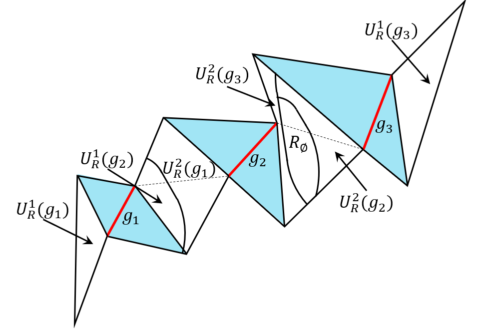
First, we consider the case in which a single guard is allocated to a triangle of the triangulation. An allocation maps each guard to a subset of triangles in the triangulation of the polygon. Let denote the set of all possible allocations. We say that an allocation is complete if there is no triangle with no guard allocated to it. Next, we classify the triangles of the triangulation of (the triangles in ) based on the number of incident guards and their position relative to the triangles. Refer to Figure 1. The red segments in the figure represent the diagonals on which the guards move. In the subsequent figures, those diagonals are labeled as instead.
- 1.
Safe Triangle: A triangle is called safe if covers at all times regardless of the location of . Clearly, if there is a guard deployed on one of the edges of , the triangle is a safe one. We use to denote the set of safe triangles. In Figure 1, safe triangles are shaded in blue.
- 2.
Unsafe Triangle: A triangle is called unsafe if , where is the cardinality operator. In Figure 1, unsafe triangles are shaded in orange.
- 3.
Regular Triangle: A triangle is regular if it is neither safe nor unsafe. In Figure 1, regular triangles are shaded in white.

Let denote the set of triangles that are incident to the endpoint of (). Also, let denote the set of non-safe (RegularUnsafe) triangles in and denote the set of non-safe triangles that are incident to . By definition, is always covered by for every allocation . We want to assign a to every so that can cover when the intruder lies in it. Clearly, only the guards in can be assigned to . The deployment strategy proposed in Section 3.1 guarantees that for every . Therefore, an allocation that assigns a guard to each triangle in exists. Moreover, every unsafe triangle can only be assigned to the single guard incident to it.
Given an allocation , there are two possibilities for each :
- 1.
All the non-safe triangles assigned to are in . In this case, is static, and can cover all the triangles assigned to it from regardless of the speed ratio .
- 2.
There are triangles assigned to in and . This implies that needs to be at () when the intruder lies in (). Therefore, has to move from one endpoint of to the other depending on . Assume that is initially located in any triangle assigned to , and moves to a triangle also assigned to . As a result, the guard , initially located at , moves to . Therefore, should reach before the intruder can reach . If the aforementioned condition is satisfied for every and every assigned to , then can track when it is inside any triangle allocated to it.
To summarize the above discussion, an allocation should satisfy the following conditions:
- 1.
is complete.
- 2.
Unsafe triangles are allocated to the single guard incident to them.
- 3.
, where are the sets of triangles allocated to that correspond to and respectively.
An allocation is called feasible if it satisfies the above conditions. Given the constraint that a single guard can be allocated to a non-safe triangle, we pose the following problem:
Problem 1: Given , what is the minimum value of and the corresponding allocation for which the intruder can be persistently tracked?
encodes the adjacency between faces of based on common diagonals. Analogous to a dual graph, we define a Guard Adjacency Graph (GAG), denoted as , which encodes the adjacency between faces of the triangulation graph based on common guards. For a given triangulation graph of the polygon and deployment of the guards, is constructed as follows. Each vertex of corresponds to an non-safe triangle in . An edge exists between vertices and in if there exists a guard such that and . The weight of the edge is given by .
Next, we define terms related to allocation of guards to triangles. Given an allocation , let be the set of triangles assigned to . Then we define the cost of the allocation of as . The overall cost of the allocation for is defined as . Based on these definitions, Problem can be formulated as the following problem on :
UNIALLOC: Find a feasible allocation for which is minimized.
In order to prove the above theorem, first we define a set of representatives from . For each non-safe triangle , we define a set . is a collection of disjoint sets. For any and with and guards , define as follows:
| (1) |
for models the fact that and can cover and , respectively, by staying static at the corresponding endpoints. If and , and are are located at opposite ends of . In this case, should have a minimum speed of to cover triangles and if the intruder moves between them along the shortest path between them. Finally, and implies that and are incident to the same endpoint of . Since can cover both triangles from that endpoint, it can remain static. Therefore, in that case.
We say that a set is a set of representatives if for all . Based on the definition of a set of representatives, we define the following problem which is equivalent to UNIALLOC:
MAXREP: Find the set for which is minimized.
The following problem casts MAXREP as a decision problem:
GAMMAREP: Given , does there exist a set of representatives of size such that for all with ?
The next lemma proves that GAMMAREP is NP-hard which in turn implies that MAXREP is at least NP-hard.
Lemma 1
GAMMAREP is NP-hard.
Proof
We reduce the problem of finding a -clique [75] in a graph (a NP-hard problem [76]) to GAMMAREP. Consider a graph without self-loops such that . The problem of finding a -clique in is NP-hard [77]. For each , we define a set . For a pair of vertices , we define the following cost function:
| (2) |
Given sets and the cost function stated above, we prove that a -clique in exists if and only if a set of representatives such that can be found.
( First, assume that there exists such a but there is no -clique in . By definition, for each pair , , and ( implies that has a self-loop which is not possible). Therefore, each is associated to a different . Since there is no -clique in , the subgraph induced by the vertices associated with is not complete. Therefore, there is at least one pair such that there is no edge shared between and in which implies (a contradiction). Therefore, if there exists of size such that for all then a -clique in exists.
() Now assume that there is no which meets the aforementioned constraints, but there is a -clique in . Since contains a -clique, there is a subset of vertices such that its induced subgraph is complete. Since is complete, choosing for each as an element of implies that for any , an edge exists between and in . Therefore, for every which contradicts the assumption that there is no of size such that for all . Therefore, if there exists a -clique in then there is of size such that for all , and the reduction can be done in polynomial time. Thus, we have a polynomial-time reduction from -clique to GAMMAREP.
Based on the above discussion, we can state the following theorem.
Theorem 4.1
UNIALLOC is NP-hard.
Proof
The proof follows from the fact UNIALLOC is equivalent to MAXREP which is at least NP-hard.
4.1 Suboptimal Algorithm for Computing Approximate minimum speed ratio
MAXCLIQUE refers to the problem of finding the maximum-sized clique in a graph. MAXCLIQUE is NP-hard [78]. An approximation algorithm for MAXCLIQUE can be used to obtain a suboptimal solution for Problem 1. The procedure is as follows. Let be a graph such that . Recall that for all . Since (), and , . Therefore, . Additionally, let . Each edge has an associated weight defined as follows:
| (3) |
We define as a subgraph of such that and . Therefore, consists of edges in with weights less than or equal to . We can use any approximation algorithm for MAXCLIQUE to find a clique in for a given . Since , we perform the aforementioned check for values of that correspond to the weights of the edges in . The suboptimal allocation corresponds to the minimum value of for which a clique is found in the graph . If no such is found, is equal to the minimum . Each vertex in the clique corresponds to a distinct triangle in , and each one of them corresponds to a which is the guard assigned to . This gives an approximate optimal allocation for each .
It has also been shown that approximating the MAXCLIQUE within a factor of for some is NP-hard [79, 80]. In the past, probabilistic techniques [81, 82, 83, 78] have been proposed in the literature to find largest cliques without any guarantees on the optimality. [84] presents an approximation algorithm that finds a clique with an approximation ratio of when the size of the maximum clique is between and . Since , where is the number of vertices of the polygon, the performance ratio in our case is .
Next, we consider the case in which more than one guard can be assigned to each non-safe triangle. In this case, we partition into disjoint regions, each covered by a unique guard (incident on ). The problem of computing the minimum guard speed () when multiple guards can be assigned to a single triangle is as hard as UNIALLOC which itself is NP-hard.
In the next section, we address the problem of allocating guards to triangles for a given maximum speed of the intruder and the guards.
5 Computing a Feasible Allocation for Known Guard Speed
In the previous section, we proved that the problem of finding the minimum speed of the guards that can ensure tracking is NP-hard. In this section, we propose a technique to search and compute a feasible allocation for given maximum speed of the intruder and guards. Therefore, the speed ratio is known. We address the general allocation problem in which multiple guards can be assigned to cover an unsafe triangle in the polygon. Specifically, we focus on techniques that partition the polygon, and activate guards to track an intruder located in its allocated partition.
Let denote the region inside triangle assigned to the guard incident to vertex (). We define as the set of regions assigned to that can be covered from . We define as the union of the regions belonging to . Let denote the region assigned to . The cost associated with an assignment is defined as .
In this section, we address the following problem:
Problem 2: For the deployment of guards inside a polygon described in Section 3.1 and a given , determine for each such that , and the region in which the intruder lies can be covered by the guard allocated to it.
Since ,, for all . Let denote the maximum distance traveled by the intruder during the time in which can travel from one endpoint of to the other.
In the next section, we present the procedure to find .
5.1 Sequential computation of partitions
The allocation algorithm proposed in the next section sequentially computes for each guard . The end point of at which is computed first gets the label . Subsequently, is computed at the other end point of which is assigned the label .
From the definition of , it is clear that must be defined for every for computing . Based on the classification of , we can have the following scenarios:
- 1.
If every is an unsafe triangle, by definition since can only be covered by . In this case, .
- 2.
If is a regular triangle, can be computed only if the region allocated to other guards incident to is known. In this case, , where is the complement of .
The following equation allows computing from :
| (4) |
where is an open ball (using the metric defined in Section 1) of radius centered at , and is its complement. Also, is the region inside that has not yet been assigned to a guard. In the absence of obstacles between and :
| (5) |
where is an open ball in , denotes the Minkowski sum, and is the complement of the Minkowski sum. The set is called the offset of . The offset of a set bounded by a polyline curve (line-segments/arcs of circle) is a set bounded by polyline curve [85]. Appendix A shows that and are sets bounded by polyline curves even in the presence of obstacles. From and , we can compute using the equation .
In Figure 2, there are three guards, , , and . All the non-safe triangles incident to one endpoint of the diagonals of and are unsafe triangles. Therefore, and are as shown in the figure. However, that is not the case for . In order to define , either or needs to have a region assigned to it in the triangles shared between it and . In Figure 2, (which is obtained from (4)) is used to define , which in turn is used to define using (4). Once that all the guards in have been assigned to a region , it is possible to determine if no allocation was found for the given . By definition, a region inside ensures that every location within the triangle is assigned to a guard in . However, that may not hold if all the regions allocated to the guards in are . Every is constructed using (4), thereby, guaranteeing that is assigned to the largest possible region within such that . Otherwise, there is no guarantee to keep track of the intruder if it follows the shortest path between and . Clearly, an allocation cannot be found by the above process if there is a region inside the triangle that is not assigned to any guard in after every is defined for . In Figure 2, there is a region inside the regular triangles shared by and that cannot be assigned to those guards. The existence of a region implies that an allocation that guarantees successful tracking was not found. The blue shaded triangles correspond to safe triangles, which by definition are covered all the time.
5.2 Guard Allocation
In this section, we present an allocation algorithm that respects the constraints in Problem 2. Algorithm 2 presents the pseudocode of the allocation technique. Given a triangulation graph and the speed ratio as the input, Algorithm 2 provides a partition of the polygon , and an allocation of the guards to the partitions. The initialization, update and termination step of Algorithm 2 are as follows:
- •
Initialization:
- –
Initialize two queues: .
- –
If there is a such that has an endpoint at which all the non-safe triangles incident to it are unsafe triangles, then is added to .
- –
If no guard satisfies the previous criteria, . A guard is selected using Algorithm 4, and all the triangles incident to one of its endpoints are assigned to it.
- –
- •
Update:
- –
If there is a guard such that for each , the regions are already defined and allocated for all . is called the preferential endpoint of , and is labeled as .
- –
A guard is selected. Algorithm 3 is used to compute and .
- –
- –
- •
Termination: The algorithm can terminate in two ways described as follows.
- –
Algorithm 3 finds a region inside a non-safe triangle . Since the region cannot be assigned to any guard, the algorithm terminates. Therefore, no allocation is found.
- –
Each is partitioned, and each partition is assigned to a guard. In this case a feasible allocation is found.
- –
Figure 3 (a) shows a polygonal environment with () edges and () guards. There are safe and non-safe triangles. The corresponding graph is shown in Figure 3 (c). The orientation of the edges of illustrates a partial order in which the vertices of are allocated by the algorithm. has vertices, each one associated with an non-safe triangle. Edges exist between vertices that correspond to triangles incident to opposite endpoints of the diagonal of a guard. For example, and are incident to one endpoint of and is incident to the other. Hence, edges in that correspond to are and . In Algorithm 2, once a is chosen (and is obtained by Algorithm 3), the endpoints of its diagonal can be labeled as and .
In the example shown in Figure 3, when the algorithm starts, . meets the definition of the queue since all the non-safe triangles incident to one endpoint of are unsafe triangles ( and ). The same is true for one endpoint of ( is an unsafe triangle). Next, is selected and its corresponding preferential endpoint is named . Algorithm 3 is called. It uses the procedure to compute from Section 5.1 for a given . Thus, and , and . Edges , , and become outgoing edges of , and edges , , and become outgoing edges of . Next, the regions that correspond to the endpoint are computed. They are , , and which is the region inside assigned to shown in Figure 3 (b). Finally, the algorithm searches for the existence of any region with . Since it is not found, the process returns to Algorithm 2 where (which contains all guards that have been allocated) and are updated to and . In the second iteration, is selected, and the same process is repeated. . Edges and become outgoing edges of edges of . and (the region inside assigned to shown in Figure 3 (b)) are obtained. At the end of the iteration, and . The algorithm continues until the end of the fourth iteration at which point and . The allocation of all the regions of the environment is shown in Figure 3 (b), and the resulting directed graph is illustrated in Figure 3 (c). Notice that Line of Algorithm 3 is only reached when all the edges incident to a vertex in are incoming edges. Thus, the regions and for each guard are already defined. Therefore, the algorithm checks whether the triangle is completely covered by the regions allocated to the guards or there is a region inside the triangle that cannot be assigned to guards. In the example, the aforementioned check is performed for triangles , , , , and . We can see that for all the other vertices, there are outgoing edges incident to them, and those edges are associated with a single guard. According to the definition of , at each iteration Algorithm 2 selects a guard such that the regions of the other guards that can cover the triangles in are already defined. It follows that Algorithm 4 selects the vertices that correspond to the triangles in and orients all the edges incident to them that correspond to as outgoing edges of those vertices. Since all the other guards that can cover those triangles had their regions defined, it means that Algorithm 4 was called before to orient their edges so all of those edges are outgoing edges of other vertices. Hence, they are incoming edges of the vertices associated with the triangles in . This explains why either all the edges incident to a vertex in become incoming edges, or only the edges associated to one guard become outgoing edges.


If and (Line ), Algorithm 2 calls Algorithm 4 to allocate the guards in . It happens when the iterative procedure cannot find a unique allocation for the non-safe triangles that can be covered by the guards in the set . Let denote the triangles that can be covered by the guards in such that they contain regions that have not yet been assigned. Let be the set of vertices in that correspond to the triangles in . Triangles in contain regions that can be assigned to more than one guard, and hence, it is not possible to determine a unique partition. Thus, for each there are at least two guards with non-oriented edges incident to .


Figure 4 shows such a scenario involving guards and non-safe triangles. If Algorithm 3 was executed, it could find or , or also or . The presence of the regular triangles and prevents Algorithm 3 to find and . There is no region that has initially been assigned to any of the guards inside and which can be used to construct the region of the other guard. Therefore, and . Let be the subgraph induced by . We know that there are at least two guards with non-oriented edges incident to each . Since the number of vertices of is finite ( cannot be a tree with an infinite length path), each is inside a cycle involving the diagonal of guards in . Otherwise, if there is a with only one neighbor in , there is only one guard with a non-oriented edge incident to it which implies . In Figure 4 (c), is the graph induced by and . It is a cycle of length with edges and .
Algorithm 4 resolves the aforementioned deadlock in . It arbitrarily selects a and an endpoint of . Subsequently, it assigns to all the unassigned regions that it can cover from the selected endpoint. Thus, the edges of the other guards in that can cover those regions are deleted from . Consequently, meets the requirement to get added to which in turn allows Algorithm 2 to continue. In the example of Figure 4, Algorithm 4 arbitrarily selects and the endpoint that is a vertex of is chosen as . Thus, the edges and are deleted from , and , so Algorithm 2 can continue. Next is chosen, and Algorithm 3 finds , , and . Thus, edges and become outgoing edges of , and and become outgoing edges of . It follows that and is the region inside assigned to shown in Figure 4 (b). At the end of this iteration, and . At the end of the second iteration all the regions of the environment have been assigned as shown in Figure 4 (b). The resulting directed graph is illustrated in Figure 4 (c) in which the edges deleted by Algorithm 4 are shown as dotted segments.
Since the number of edges in that can be associated to a given guard is upper bounded by , the time complexity of Algorithm 3 is . Also, since the total number of edges that can be deleted is upper bounded by , the time complexity of Algorithm 4 is . At each iteration of Algorithm 2, one guard enters and Algorithm 3 is called. It follows that the time complexity of Algorithm 2 is .
5.3 Completeness and Correctness of GENALLOC
The following lemma proves that Algorithm 2 terminates.
Lemma 2
Algorithm 2 terminates in a finite number of steps.
Proof
The next lemma states a condition under which Algorithm 2 is complete.
Lemma 3
If is a forest, Algorithm 2 is complete.
Proof
The proof is by contradiction. Consider a polygonal environment for which is a forest, and Algorithm 2 fails to find a feasible allocation of guards even though one exists. From hereon, any variable with a symbol on top of it is associated with the feasible allocation. For example, denotes a region in assigned to based on the feasible allocation. Since Algorithm 4 cannot find a feasible allocation in , it terminates at Line . Hence, there is a vertex such that all the edges incident to are incoming edges, and the triangle has a region which by definition cannot be assigned to any guard by Algorithm 4. Since a feasible allocation exists, every point inside can be assigned to a guard in . Let denote the region that can be covered by a guard in the feasible allocation. Therefore, exists such that and . For the feasible allocation, . Since , . By definition, . Therefore, a region exists such that and . Therefore, . Hence, there exists a guard and a region such that and . Therefore, we can find a sequence of vertices and guards in such that , and corresponding regions such that and . The sequence terminates if in which case is an unsafe triangle. Since does not exist . Since and , we arrive at a contradiction. If the sequence does not terminate, then there exist and such that since the number of vertices in are finite. This implies the existence of a cycle in . Therefore, we arrive at a contradiction since is a forest.
In the appendix (Lemma 8), we prove a more general result which shows that Algorithm 2 is complete if Algorithm 4 is never called during execution. Figure 5 shows an example in which does not contain cycles. In Figure 5 (a), a simple polygonal environment is shown along with the deployment of guards. There are four non-safe triangles , , and . and can be covered by . and can be covered by . In Figure 5 (b), the corresponding graph is shown. is a forest that consists of two paths. Lemma 3 states that Algorithm 2 will always find the feasible allocation for this environment.


5.4 Classification of Guards
In this section, we present a classification of the guards. It is based on the regions constructed from Algorithm 2.
- 1.
Type guard: These are guards for which either or . Since the region allocated to a type guard can be covered from one endpoint of its diagonal, it is a static guard.
- 2.
Type guard: There are guards for which all the non-safe triangles allocated to the guard incident to one endpoint are unsafe triangles. Notice that each edge in that corresponds to a type guard is an outgoing edge of a vertex such that . Clearly, if for each , then is a type guard.
- 3.
Type guard: Any guard which is neither Type nor Type is a Type 2 guard.
Consider the example shown in Figure 6. Assume , and are the only non-safe triangles incident to , and respectively. Algorithm 2 selects the non-safe triangle to be assigned to the only guard that can cover it (). Since , is a type guard. Once is computed after a few steps, Algorithm 2 selects the non-safe triangle and allocates the unshaded region to . Besides , can also be covered by and . Regions and are known. Consequently, and are also computed. It follows that the unshaded region in is labeled as . Moreover, since , . It follows that is an example of a type guard.

In Algorithm 4 an unassigned guard is arbitrarily chosen to cover the unassigned regions inside the triangles incident to one of the endpoints of its diagonal. is arbitrarily chosen since Algorithm 2 failed to find a unique partition of such regions. It implies that cannot be constructed unlike in the case of a type , a type nor a type guard. However, the arbitrary allocation in Algorithm 4 assigns those regions to . As a result, is converted to a type or a type guard.
5.5 Motion strategy for the Guards
In this section, we present a motion strategy for the guards to move on their diagonals. We introduce the concept of critical curves to propose activation strategies for type and type guards.
From the discussion in the previous section, is the region assigned to a type or type guard . Therefore, it is the responsibility of to cover the triangles incident to when the intruder lies in .
We define an internal critical curve, denoted by , as the boundary of . Corresponding to an internal critical curve, we define an external critical curve as follows:
| (6) |
Comparing the definition of to the definition of (see Equation (4)), we can conclude that a part of the boundary of can belong to . We define a critical region associated with the guard as follows:
| (7) |
where is the interior of . Note that, by definition, the boundary of contains both curves and , and since , it is clear that .
Figure 7 shows the region for the guard . The neighboring guards are not shown for the sake of simplicity. , the boundary of , is represented as blue segments and arcs that form the boundary of the regions , and . Since triangles and are safe triangles (they have as an edge), there is no internal critical curve inside them. The green segments and curves denote , and the unshaded region inside is . The boundary of is formed by , and edges of the environment. The dark colored regions represent and which are part of .

For an intruder located in , the following equation maps the position of the intruder () to the position of (denoted as ) along its diagonal:
| (8) |
where is the location of vertex (). If , remains static at . Otherwise, if , remains static at .
By definition, while . Hence, (8) guarantees that will always cover the regions assigned to it when the intruder is located in them.
Consider the case of a guard such that is incident to at a vertex . The motion strategy proposed in (8) ensures that is covered if there is an intruder inside . However, if the intruder is located in , where is the interior of , cannot cover because can only be located at when the intruder is outside according to (8). Now, consider the case when is incident to at a vertex labeled . Since is a vertex of , will be covered by if there is an intruder inside it according to (8). However, if the intruder lies outside , then is not covered by since is not located at according to (8). Consequently, for each , there exists a region which prevents to cover when the intruder lies inside it. This region, denoted by , is called the extended critical region. It is given by the following expression:
| (9) |
Based on the concept of extended critical regions, Lemma 4 presents a necessary and sufficient condition for the guards to cover a non-safe triangle when an intruder lies in it.
Lemma 4
For the guards in (), (8) guarantees that the triangle is covered when an intruder is located in it if and only if .
Proof
() Assume that , and is not covered when the intruder lies in . It implies that there is a location inside for the intruder that prevents every to cover . According to (8), such a region must belong to which contradicts our assumption.
() Next, assume that and is covered when the intruder is located in it. Since when , there is no guard covering according to (8), which is a contradiction. The lemma follows.
6 Polygons with Holes
In this section, we assume that has polygonal holes which represent obstacles inside the polygon. Let represent the set of polygonal holes. Let denote the total number of vertices of , where is the number of vertices of the hole and . Figure 8 shows a polygonal environment with an internal polygonal hole . In Theorem of [28], it is shown that one can find an internal diagonal of the triangulation of between any two holes (or between a hole and the outer boundary) which merges two holes (or the hole with the boundary) if a wall of thickness is placed on the diagonal. This reduces the value of by . See Figure 8 where is merged with the outer boundary through the diagonal shared by triangles and . Therefore, for any polygon with vertices and internal polygonal holes, we can construct a simply-connected polygon with vertices. We can apply all techniques proposed in the previous sections for deploying guards, and allocating them to triangles of the triangulation of for tracking the intruder.

7 Tracking Multiple intruders
In this section, we analyze the performance of the proposed algorithm for multiple intruders. We assume that all the intruders have the same maximum speed . We use the symbol to denote the set of intruders, and the vector to denote their positions inside the polygon. We assume that the deployment of the guards and the allocation of the different regions of the environment are obtained using the techniques presented in sections 3.1 and 4, respectively.
In Section 5.5, a motion strategy for the guards was proposed for a single intruder. (8) is a reactive motion strategy that depends on the location of the intruder. It ensures that each guard can cover when the intruder is inside it. In the presence of multiple intruders, the priority for each is to cover as long as there is an intruder inside it. Hence, the motion strategy only needs to consider the intruder closer to , i.e. if there is an intruder inside , stays at regardless of the positions of other intruders. Therefore, the motion strategy of the guard in this case is given by (10), wherein is replaced by defined as follows:
| (10) |
In Section 5.5, we showed that an intruder inside each associated to will prevent anon-safe triangle from being covered by any guard incident to it. Therefore, intruders are sufficient to keep uncovered. However, if for example, there are two guards such that , a single intruder lying inside the intersection will prevent and from covering . Therefore, fewer than intruders can prevent from being covered by any guard incident to it if there are non-empty intersections between the extended critical regions corresponding to distinct guards that can cover .
Consider the power set of all guards incident to . Let be a collection of all sets for which the extended critical regions of the guards belonging to have a non-empty intersection. The problem of finding the minimum number of intruders that can be placed at the intersection of extended critical regions to uncover is equivalent to the problem of finding the minimum cover of .
Let denote the maximum number of intruders that can be tracked by the guards incident to without uncovering when there is an intruder inside it. The following lemma relates to .
Lemma 5
Let .
| (11) |
where
Proof
intruders, each placed in a distinct , are sufficient to prevent all guards incident to from covering it when an intruder is located inside . If , the intruder inside the cannot lie inside any . Therefore, in this case. Otherwise, the intruder located inside can cover an . Therefore, in this case.
Since is the minimum set cover of , intruders cannot prevent from being covered by at least one guard . Therefore, . The theorem follows.
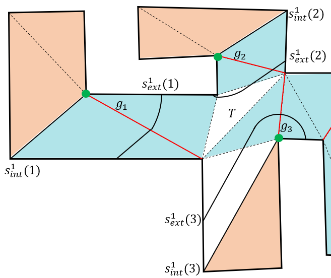
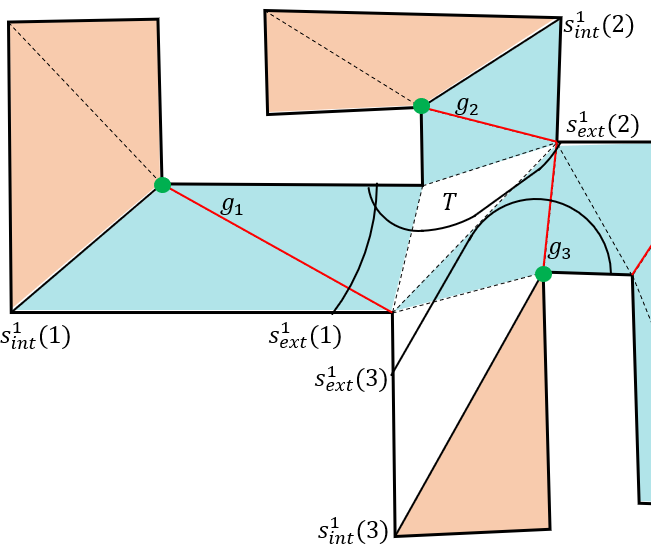
In Figure 9 9(a), two type guards and , and a type guard are shown with their corresponding external and internal critical curves. The corresponding endpoints are shown with a green disc. The regions are shaded in orange, and the safe triangles are shaded in blue. is a regular triangle that can be covered by , and . Therefore, the set consists of the external critical regions and has cardinality . Since there is no intersection between any region in and then . Figure 9 9(b), shows the same case but for a smaller value of . . This implies that consists of the extended critical region of and the intersection of the extended critical regions of and . In this case, consists of and , so it has cardinality . Since none of the regions in intersects with , then .
Theorem 7.1
The minimum number of intruders that can be tracked based on the strategy proposed in (10) is .
Proof
The set cover problem is NP-complete [75]. Several polynomial time approximation schemes (PTAS) for the set cover problem have been proposed in the literature [86, 87, 88, 89, 90, 91]. Better approximation ratios can be obtained at the expense of computational complexity slightly higher than a PTAS [92]. For example, it has been shown that any - approximation algorithm for the set cover problem must run in time at least for some small constants [93]. [94, 95] present some efforts to tighten the running time by reducing the value of in . We can use either of the aforementioned approaches to obtain . For a problem instance of large size, one might prefer a PTAS, whereas a moderately exponential algorithm is more preferable when the number of guards covering each is small enough.
8 Conclusion
In this work, we addressed the problem of tracking mobile intruders in a polygonal environment using a team of diagonal guards. Leveraging on deployment strategies for mobile coverage in art gallery problems, we proposed control and coordination strategies for the guards to track intruders inside a polygonal environment. At first, we formulated the tracking problem as a multi-robot task assignment problem on the triangulation graph of a polygon. We classified the guards based on their position with respect to the triangles of the triangulation. Next, we showed that the problem of finding the minimum speed of the guards to cover the triangles of the triangulation under the constraint that each triangle can only be covered by a single guard is NP-hard. Given the maximum speed of the intruder, we proposed an algorithm to find a feasible allocation of guards to the triangles of the triangulation when multiple guards are allowed to cover the triangle. We proved the correctness of the proposed algorithm, and its completeness for a specific set of inputs. Based on the task allocated to a guard, we proposed control laws for the guards to move along their diagonals. Finally, we extended the algorithm to address deployment and allocation strategies for non-simple polygons and multiple intruders.
We believe that our paper is a first step towards MRS deployment for persistent tracking with provable guarantees. An important direction of future research is to address the tracking problem for guards with sensing and motion constraints, for example, edge guards, which are more constrained in their motion, or line guards, which are less constrained than diagonal guards. Another future research direction is to study the tracking problem for special polygons, for example, orthogonal polygons, monotone polygons etc. For these polygons, it has been shown that fewer guards are required for coverage. Finally, the problem of tracking with mixed team of guards (static and mobile) is an interesting direction of future research.
References
- [1] S. Mittal and J. K. Rai. Wadoro: An autonomous mobile robot for surveillance. In Proceedings of IEEE International Conference on Power Electronics, Intelligent Control and Energy Systems, pages 1–6, July 2016.
- [2] S. Witwicki, J. C. Castillo, J. Messias, J. Capitan, F. S. Melo, P. U. Lima, and M. Veloso. Autonomous surveillance robots: A decision-making framework for networked multiagent systems. IEEE Robotics Automation Magazine, 24(3):52–64, Sept 2017.
- [3] T. Theodoridis and H. Hu. Toward intelligent security robots: A survey. IEEE Transactions on Systems, Man, and Cybernetics, Part C (Applications and Reviews), 42(6):1219–1230, Nov 2012.
- [4] D. Ciccimaro, H. Everett, G. Gilbreath, and T. Tran. Automated security response robot, 1999.
- [5] G. Tuna, C. Tasdemir, K. Gulez, T. V. Mumcu, and V. C. Gungor. Autonomous intruder detection system using wireless networked mobile robots. In Proceedings of IEEE Symposium on Computers and Communications, pages 1–5, July 2012.
- [6] Piotr Bazydło, Janusz Kacprzyk, and Krzysztof Lasota. Global path planning for a specialized autonomous robot for intrusion detection in wireless sensor networks (wsns) using a new evolutionary algorithm. In Wojciech Mitkowski, Janusz Kacprzyk, Krzysztof Oprzkedkiewicz, and Paweł Skruch, editors, Trends in Advanced Intelligent Control, Optimization and Automation, pages 503–513. Springer International Publishing, 2017.
- [7] G. Oriolo, G. Ulivi, and M. Vendittelli. Real-time map building and navigation for autonomous robots in unknown environments. IEEE Transactions on Systems, Man, and Cybernetics, Part B (Cybernetics), 28(3):316–333, Jun 1998.
- [8] Michael Montemerlo and Sebastian Thrun. Large-scale robotic 3-d mapping of urban structures. In Marcelo H. Ang and Oussama Khatib, editors, Experimental Robotics IX, pages 141–150, Berlin, Heidelberg, 2006. Springer Berlin Heidelberg.
- [9] N. Wright M. Majerus, R. Vanaman. Autonomous mine detection system (amds) neutralization payload module, 2010.
- [10] J. D. Nicoud and M. K. Habib. The Pemex-B autonomous demining robot: Perception and navigation strategies. In Proceedings of IEEE/RSJ International Conference on Intelligent Robots and Systems. Human Robot Interaction and Cooperative Robots, volume 1, pages 419–424 vol.1, Aug 1995.
- [11] Fahimeh Rezazadegan, Sareh Shirazi, Ben Upcrofit, and Michael Milford. Action recognition: From static datasets to moving robots. In Proceedings of IEEE International Conference on Robotics and Automation, pages 3185–3191, 2017.
- [12] O. P. Popoola and K. Wang. Video-based abnormal human behavior recognition; a review. IEEE Transactions on Systems, Man, and Cybernetics, Part C (Applications and Reviews), 42(6):865–878, Nov 2012.
- [13] Cheong Hee Lee, Soo Hyun Kim, Sung Chul Kang, Mun Sang Kim, and Yoon Keun Kwak. Double-track mobile robot for hazardous environment applications. Advanced Robotics, 17(5):447–459, 2003.
- [14] S. Yamamoto. Development of inspection robot for nuclear power plant. In Proceedings of IEEE International Conference on Robotics and Automation, pages 1559–1566 vol.2, May 1992.
- [15] Pradipta Ghosh, Andrea Gasparri, Jiong Jin, and Bhaskar Krishnamachari. Robotic wireless sensor networks. arXiv preprint arXiv:1705.05415, 2017.
- [16] Donato Di Paola, Annalisa Milella, Grazia Cicirelli, and Arcangelo Distante. An autonomous mobile robotic system for surveillance of indoor environments. International Journal of Advanced Robotic Systems, 7(1):8, 2010.
- [17] T. Sakuyama, J. Figueroa, Y. Miyazaki, and J. Ota. Transportation of a large object by small mobile robots using hand carts. In Proceedings of IEEE International Conference on Robotics and Biomimetics, pages 2108–2113, Dec 2012.
- [18] M. Dunbabin and L. Marques. Robots for environmental monitoring: Significant advancements and applications. IEEE Robotics Automation Magazine, 19(1):24–39, March 2012.
- [19] H. Afzaal and N. A. Zafar. Robot-based forest fire detection and extinguishing model. In Proceedings of International Conference on Robotics and Artificial Intelligence, pages 112–117, Nov 2016.
- [20] N. Matsuhira, F. Ozaki, S. Tokura, T. Sonoura, T. Tasaki, H. Ogawa, M. Sano, A. Numata, N. Hashimoto, and K. Komoriya. Development of robotic transportation system - shopping support system collaborating with environmental cameras and mobile robots -. In Proceedings of International Symposium on Robotics, pages 1–6, June 2010.
- [21] A. W. Y. Ko and H. Y. K. Lau. Intelligent robot-assisted humanitarian search and rescue system. International Journal of Advanced Robotic Systems, 6(2):12, 2009.
- [22] Steve Fisk. A short proof of Chvátal’s Watchman Theorem. Journal of Combinatorial Theory, Series B, 24(3):374, 1978.
- [23] J. Kahn, M. Klawe, and D. Kleitman. Traditional galleries require fewer watchmen. SIAM Journal on Algebraic Discrete Methods, 4(2):194–206, 1983.
- [24] Stephane Durocher, Omrit Filtser, Robert Fraser, Ali D. Mehrabi, and Saeed Mehrabi. Guarding orthogonal art galleries with sliding cameras. Computational Geometry, 65:12 – 26, 2017.
- [25] Stephane Durocher, Omrit Filtser, Robert Fraser, Ali D. Mehrabi, and Saeed Mehrabi. A (7/2)-approximation algorithm for guarding orthogonal art galleries with sliding cameras. In Alberto Pardo and Alfredo Viola, editors, LATIN 2014: Theoretical Informatics, pages 294–305, Berlin, Heidelberg, 2014. Springer Berlin Heidelberg.
- [26] Stephane Durocher and Saeed Mehrabi. A 3-approximation algorithm for guarding orthogonal art galleries with sliding cameras. In Kratochvíl Jan, Mirka Miller, and Dalibor Froncek, editors, Combinatorial Algorithms, pages 140–152, Cham, 2015. Springer International Publishing.
- [27] Mark de Berg, Stephane Durocher, and Saeed Mehrabi. Guarding monotone art galleries with sliding cameras in linear time. Journal of Discrete Algorithms, 44:39 – 47, 2017.
- [28] Joseph O’Rourke. Art gallery theorems and algorithms. Oxford University Press, New York, NY, 1987.
- [29] Frank Hoffmann. On the rectilinear art gallery problem. In Michael S. Paterson, editor, Automata, Languages and Programming: Proceedings of 17th International Colloquium Warwick University, England, pages 717–728. Springer Berlin Heidelberg, Berlin, Heidelberg, 1990.
- [30] J. Czyzowicz, E. Rivera-Campo, N. Santoro, J. Urrutia, and J. Zaks. Guarding rectangular art galleries. Discrete Applied Mathematics, 50(2):149 – 157, 1994.
- [31] Jorge Urrutia. Art gallery and illumination problems. In Handbook of Computational Geometry, pages 973–1027. North-Holland, 2000.
- [32] Joseph O’Rourke. Galleries need fewer mobile guards: A variation on Chvátal’s theorem. Geometriae Dedicata, 14(3):273–283, 1983.
- [33] Godfried T. Toussaint. Computational geometric problems in pattern recognition. In Josef Kittler, King Sun Fu, and Louis-François Pau, editors, Pattern Recognition Theory and Applications, pages 73–91, Dordrecht, 1982. Springer Netherlands.
- [34] Paul Colley, Henk Meijer, and David Rappaport. Motivating lazy guards. In Proceedings of the Canadian Conference on Computational Geometry, pages 121–126, 1995.
- [35] David C. Kay and Merle D. Guay. Convexity and a certain property Pm. Israel Journal of Mathematics, 8(1):39–52, Mar 1970.
- [36] Salma Sadat Mahdavi, Saeed Seddighin, and Mohammad Ghodsi. Covering orthogonal polygons with sliding k-transmitters. In Proceedings of the Canadian Conference on Computational Geometry. Citeseer, 2014.
- [37] Pooyan Fazli, Alireza Davoodi, Philippe Pasquier, and Alan K Mackworth. Fault-tolerant multi-robot area coverage with limited visibility. In Proceedings of the Workshop on Search and Pursuit/Evasion in the Physical World: Efficiency, Scalability, and Guarantees, 2010.
- [38] P. Fazli, A. Davoodi, P. Pasquier, and A. K. Mackworth. Complete and robust cooperative robot area coverage with limited range. In Proceedings of IEEE/RSJ International Conference on Intelligent Robots and Systems, pages 5577–5582, Oct 2010.
- [39] D. Lee and A. Lin. Computational complexity of art gallery problems. IEEE Transactions on Information Theory, 32(2):276–282, Mar 1986.
- [40] Subir Kumar Ghosh. Approximation algorithms for art gallery problems in polygons. Discrete Applied Mathematics, 158(6):718 – 722, 2010.
- [41] Yoav Amit, Joseph S. B. Mitchel, and Eli Packer. Locating guards for visibility coverage of polygons. International Journal of Computational Geometry and Applications, 20(5):601–630, 2010.
- [42] D. P. Barnes and J. O. Gray. Behaviour synthesis for co-operant mobile robot control. In Proceedings of International Conference on Control, volume 2, pages 1135–1140, March 1991.
- [43] Brian P. Gerkey and Maja J. Mataria. A formal analysis and taxonomy of task allocation in multi-robot systems. The International Journal of Robotics Research, 23(9):939–954, 2004.
- [44] L. E. Parker and B. A. Emmons. Cooperative multi-robot observation of multiple moving targets. In Proceedings of IEEE International Conference on Robotics and Automation, volume 3, pages 2082–2089 vol.3, Apr 1997.
- [45] Lynne E Parker. Distributed algorithms for multi-robot observation of multiple moving targets. Autonomous robots, 12(3):231–255, 2002.
- [46] P.
- [47] A. Kolling and S. Carpin. Multirobot cooperation for surveillance of multiple moving targets - a new behavioral approach. In IEEE International Conference on Robotics and Automation, pages 1311–1316, 2006.
- [48] A. Kolling and S. Carpin. Cooperative observation of multiple moving targets: An algorithm and its formalization. The International Journal of Robotics Research, 29(9):935–953, 2007.
- [49] B. B. Werger and M. J. Matarić. Broadcast of local eligibility for multi-target observation. In Distributed autonomous robotic systems 4, pages 347–356. Springer, 2000.
- [50] J. R. Spletzer and C. J. Taylor. Dynamic sensor planning and control for optimally tracking targets. The International Journal of Robotics Research, 22(1):7–20, 2003.
- [51] Z. Xu, R. Fitch, J. Underwood, and S. Sukkarieh. Decentralized coordinated tracking with mixed discrete-continuous decisions. Journal of Field Robotics, 30(5):717–740, 2013.
- [52] Volkan Isler, Sanjeev Khanna, John Spletzer, and Camillo J. Taylor. Target tracking with distributed sensors: The focus of attention problem. Computer Vision and Image Understanding, 100(1):225 – 247, 2005.
- [53] D. Goossens, S. Polyakovskiy, F. Spieksma, and G. J. Woeginger. The focus of attention problem. Algorithmica, 74(2):559–573, 2016.
- [54] Philip Dames, Pratap Tokekar, and Vijay Kumar. Detecting, localizing, and tracking an unknown number of moving targets using a team of mobile robots. The International Journal of Robotics Research, 36(13-14):1540–1553, 2017.
- [55] Karol Hausman, Jörg Müller, Abishek Hariharan, Nora Ayanian, and Gaurav S Sukhatme. Cooperative multi-robot control for target tracking with onboard sensing. The International Journal of Robotics Research, 34(13):1660–1677, 2015.
- [56] Boyoon Jung and Gaurav S. Sukhatme. Tracking anonymous targets using a robotics sensor network. In Proceedings of Association for the Advancement of Artificial Intelligence Spring Symposium. AAAI Press, 2002.
- [57] S. Markov and S. Carpin. A cooperative distributed approach to target motion control in multirobot observation of multiple targets. In Proceedings of IEEE/RSJ International Conference on Intelligent Robots and Systems, pages 931–936, Oct 2007.
- [58] Zhijun Tang and Umit Ozguner. Motion planning for multitarget surveillance with mobile sensor agents. IEEE Transactions on Robotics, 21(5):898–908, 2005.
- [59] C. Nam and D. A. Shell. Assignment algorithms for modeling resource contention and interference in multi-robot task-allocation. In Proceedings of IEEE International Conference on Robotics and Automation, pages 2158–2163, May 2014.
- [60] B. P. Gerkey and M. J. Mataric. Multi-robot task allocation: Analyzing the complexity and optimality of key architectures. In Proceedings of IEEE International Conference on Robotics and Automation, volume 3, pages 3862–3868, Sept 2003.
- [61] Lynne E. Parker. Cooperative robotics for multi-target observation. Intelligent Automation & Soft Computing, 5(1):5–19, 1999.
- [62] S. C. Botelho and R. Alami. M+: A scheme for multi-robot cooperation through negotiated task allocation and achievement. In Proceedings of IEEE International Conference on Robotics and Automation, volume 2, pages 1234–1239, 1999.
- [63] Brian P. Gerkey and Maja J. Matarić. Principled communication for dynamic multi-robot task allocation. In Daniela Rus and Sanjiv Singh, editors, Experimental Robotics VII, pages 353–362, Berlin, Heidelberg, 2001. Springer Berlin Heidelberg.
- [64] Anthony Stentz and M Bernardine Dias. A free market architecture for coordinating multiple robots. Technical Report CMU-RI-TR-99-42, Carnegie Mellon University, Pittsburgh, PA, December 1999.
- [65] L. Chaimowicz, M. F. M. Campos, and V. Kumar. Dynamic role assignment for cooperative robots. In Proceedings of IEEE International Conference on Robotics and Automation, volume 1, pages 293–298, 2002.
- [66] Kristina Lerman, Chris Jones, Aram Galstyan, and Maja J Matarić. Analysis of dynamic task allocation in multi-robot systems. The International Journal of Robotics Research, 25(3):225–241, 2006.
- [67] Zhi Yan, Nicolas Jouandeau, and Arab Ali Chérif. Multi-robot decentralized exploration using a trade-based approach. In Proceedings of International Conference on Informatics in Control, volume 2, Jan 2011.
- [68] Torbjarn S. Dahl, Maja Mataria, and Gaurav S. Sukhatme. Multi-robot task allocation through vacancy chain scheduling. Robotics and Autonomous Systems, 57(6):674 – 687, 2009.
- [69] H. Hanna. Decentralized approach for multi-robot task allocation problem with uncertain task execution. In Proceedings of IEEE/RSJ International Conference on Intelligent Robots and Systems, pages 535–540, Aug 2005.
- [70] N. Michael, M. M. Zavlanos, V. Kumar, and G. J. Pappas. Distributed multi-robot task assignment and formation control. In Proceedings of IEEE International Conference on Robotics and Automation, pages 128–133, May 2008.
- [71] Stephane Durocher and Saeed Mehrabi. Guarding orthogonal art galleries using sliding cameras: Algorithmic and hardness results. In Krishnendu Chatterjee and Jirí Sgall, editors, Mathematical Foundations of Computer Science 2013, pages 314–324, Berlin, Heidelberg, 2013. Springer Verlag.
- [72] Dietmar Schuchardt and Hans-Dietrich Hecker. Two NP-hard art-gallery problems for ortho-polygons. Mathematical Logic Quarterly, 41(2):261–267, 1995.
- [73] Stephan Eidenbenz. Inapproximability results for guarding polygons without holes. In Kyung-Yong Chwa and Oscar H. Ibarra, editors, Algorithms and Computation, pages 427–437, Berlin, Heidelberg, 1998. Springer Berlin Verlag.
- [74] Mohammad AlMahmud et al. Algorithms for minimum length sliding camera problem. Master’s thesis, Bangladesh University of Engineering and Technology, 2016.
- [75] Richard M. Karp. Reducibility among combinatorial problems, pages 85–103. Springer US, Boston, MA, 1972.
- [76] Jianer Chen, Benny Chor, Mike Fellows, Xiuzhen Huang, David Juedes, Iyad A. Kanj, and Ge Xia. Tight lower bounds for certain parameterized NP-hard problems. Information and Computation, 201(2):216 – 231, 2005.
- [77] Michael R Garey and David S Johnson. Computers and intractability, volume 29. W. H. Freeman New York, 41 Madison Avenue. New York. NY, 2002.
- [78] Panos M Pardalos and Jue Xue. The maximum clique problem. Journal of Global Optimization, 4(3):301–328, 1994.
- [79] Sanjeev Arora, Carsten Lund, Rajeev Motwani, Madhu Sudan, and Mario Szegedy. Proof verification and the hardness of approximation problems. Journal of the ACM (JACM), 45(3):501–555, 1998.
- [80] Johan Håstad. Clique is hard to approximate withinn1- . Acta Mathematica, 182(1):105–142, 1999.
- [81] Luitpold Babel. Finding maximum cliques in arbitrary and in special graphs. SIAM Journal on Computing, 46(4):321–341, 1991.
- [82] Egon Balas and Jue Xue. Weighted and unweighted maximum clique algorithms with upper bounds from fractional coloring. Algorithmica, 15(5):397–412, 1996.
- [83] David R Wood. An algorithm for finding a maximum clique in a graph. Operations Research Letters, 21(5):211–217, 1997.
- [84] Uriel Feige. Approximating maximum clique by removing subgraphs. SIAM Journal on Discrete Mathematics, 18(2):219–225, 2004.
- [85] Xu-Zheng Liu, Jun-Hai Yong, Guo-Qin Zheng, and Jia-Guang Sun. An offset algorithm for polyline curves. Computers in Industry, 58(3):240 – 254, 2007.
- [86] V. Chvátal. A greedy heuristic for the set-covering problem. Mathematics of Operations Research, 4(3):233–235, August 1979.
- [87] Rajiv Gandhi, Eran Halperin, Samir Khuller, Guy Kortsarz, and Aravind Srinivasan. An improved approximation algorithm for vertex cover with hard capacities. Journal of Computer and System Sciences, 72(1):16 – 33, 2006.
- [88] Olivier Goldschmidt, Dorit S. Hochbaum, and Gang Yu. A modified greedy heuristic for the set covering problem with improved worst case bound. Information Processing Letters, 48(6):305 – 310, 1993.
- [89] David S. Johnson. Approximation algorithms for combinatorial problems. Journal of Computer and System Sciences, 9(3):256 – 278, 1974.
- [90] L. Lovász. On the ratio of optimal integral and fractional covers. Discrete Mathematics, 13(4):383 – 390, 1975.
- [91] Petr Slavák. A tight analysis of the greedy algorithm for set cover. Journal of Algorithms, 25(2):237 – 254, 1997.
- [92] N. Bourgeois, B. Escoffier, and V.Th. Paschos. Efficient approximation of min set cover by moderately exponential algorithms. Theoretical Computer Science, 410(21):2184 – 2195, 2009.
- [93] Dana Moshkovitz. The projection games conjecture and the NP-hardness of ln n-approximating set-cover. In Anupam Gupta, Klaus Jansen, José Rolim, and Rocco Servedio, editors, Approximation, Randomization, and Combinatorial Optimization. Algorithms and Techniques, pages 276–287, Berlin, Heidelberg, 2012. Springer Berlin Verlag.
- [94] Marek Cygan, Lukasz Kowalik, Marcin Pilipczuk, and Mateusz Wykurz. Exponential-time approximation of hard problems. Computing Research Repository, abs/0810.4934, 2008.
- [95] Marek Cygan, Lukasz Kowalik, and Mateusz Wykurz. Exponential-time approximation of weighted set cover. Information Processing Letters, 109(16):957 – 961, 2009.
- [96] Ron Wein. Exact and approximate construction of offset polygons. Computer-Aided Design, 39(6):518 – 527, 2007.
- [97] Kurt Mehlhorn and Stefan Näher. LEDA: A Platform for Combinatorial and Geometric Computing. Cambridge University Press, 1999.
- [98] B.K. Choi and S.C. Park. A pair-wise offset algorithm for 2d point-sequence curve. Computer-Aided Design, 31(12):735 – 745, 1999.
- [99] Jian-She Li and Xue-Jun Ye. Offset of planar curves based on polylines. Journal of Institute of Command and Technology, 1:1–9, 2001.
Appendix A Construction of and
Obtaining all the regions yields the set and the region .
We claim that in general, the boundary of any region , denoted by , consists of arcs of circle. Let be the set of arcs of circle of . For each , we also define as the center of the circle generating (center at infinite in the case of a line segment), as its radius. We define the expanded boundary of as . Lemma 6 shows that consists only of arcs of circle grouped in a set , and Lemma 7 shows that the boundary of and consist of arcs of circle.
It is important to make this remark since most of the computational geometry libraries include segments and circle arcs as basic classes, which are required to build regions and . Some computational geometry libraries such as CGAL [96] and [97], include the implementation of approximation techniques to compute offset curves of polygons. For the case of offsets of polylines there are some approximation algorithms [85, 98, 99] which may be implemented using the aforementioned libraries with their line segment and circle classes. For this paper we used the LEDA library in the simulations.
Lemma 6
Given , its corresponding consists of arcs of circle.
Proof
Trivially, if there are no obstacles between and , is the offset of (with as the offset distance). Therefore, must be a polyline curve [85].
The presence of obstacles between and implies that the shortest path from some points in to is a chain of connected line segments instead of a line segment, as in the case where there are no obstacles between and . In Figure 10 a region is shown as an orange triangle, its corresponding is a black dotted segment, is represented as a dotted curve divided into four arcs of circle. illustrates the case of points in such that the shortest path between them and is a line segment. Now consider the presence of an obstacle implies that for all the points in , such as the one illustrated as a black circle, the shortest path between and consists of two connected line segments, one with endpoints in and vertex and other with as an endpoint and the other at . Also, for the points in , the shortest path between and consists of three connected line segments, one from to , another from to and the last one from to . Consider the points for which the shortest path between them and is not a line segment due to the presence of reflex vertices of the environment. As we can see in Figure 10, for any of such points, the shortest path from to must visit first a reflex vertex ( or for instance) of the environment. Clearly, the union of such points for which the first segment of the shortest path between them and has as an endpoint, is a subset of the union of all points in the plane that are equidistant to . Thus, they form an arc of circle, which is centered at with radius , where is the length of the shortest path between and . Therefore, every point in belongs to an arc of circle, so is the union of a set of arcs of circle.

Lemma 7
Every and is bounded by arcs of circle.
Proof
Assume that is bounded by arcs of circle. According to (4), where , is the intersection of and the complement of the region enclosed by and . Hence the boundary of consists of arcs of circle in and the edges of (arcs of circle with center at infinity). Since the boundary of consists of arcs of circle, it follows that also consists of arcs of circle from the definition of . Consider the base case where is the union of unsafe triangles. is then a set of line segments, and the lemma holds. Consider the case of an unassigned guard such that all the guards have their regions and defined for each , where . We assume that the result holds for the regions of those guards . Since the regions of those guards are defined, then and each can be defined. Recall that , where . Each is an intersection of regions which are bounded by arcs of circle. Hence, the intersection region is also bounded by arcs of circle, which trivially implies that also consists of arcs of circle. And according to the first part of this proof, it follows that consists of arcs of circle.
Appendix B Generalization of Lemma 3
Lemma 8
Proof
The proof is by contradiction. We assume that Algorithm 2 does not find a feasible allocation but there exists one. Additionally, we assume that Algorithm 4 is never called during execution. In the proof of Lemma 3, we show the existence of a sequence of vertices and guards in such that and such that and . It is also stated that the sequence terminates if in which case is an unsafe triangle. The problem of finding the existence of an allocation that works when Algorithm 2 fails is reduced to the problem of showing that the aforementioned sequence of vertices and guards in does not terminate. Since the number of vertices in is finite, the sequence is stuck in a cycle of vertices of . According to the definition of there should be a cycle in involving the vertices and the guards of the cycle in the sequence. Now we prove that such a cycle cannot exist unless Algorithm 4 was called. First, we show that for the first vertex of the cycle that appears in the sequence, , the pair of edges in incident to it are both incoming edges. If is the vertex that corresponds to the triangle where Algorithm 4 determined that it could not find an allocation, the claim is trivially proved since all edges incident to are incoming edges. Otherwise, if is no such a vertex, then it corresponds to a vertex where all the incident edges are incoming edges excepting the edges that correspond to guard . Notice that the sequence follows a direction opposite to the orientation of the edges. Therefore, when the sequence is in , the next guard cannot be . It implies that both edges of incident to do not correspond to , so they are by definition incoming edges. The sequence then continues with a different guard followed by a vertex . By definition, the edge in incident to that corresponds to is an outgoing edge, so the next edge in corresponds to a different guard and its corresponding edge in is an incoming edge of . Clearly, every vertex in has an outgoing and an incoming edge. Since is a cycle, vertex is eventually reached. However, it does not have an incoming and an outgoing edge in (both are incoming edges), which is not possible. Therefore, such a cycle does not exist in . This contradicts the initial definition of . Thus, at least one edge of was removed during the execution of Algorithm 2. This implies that Line of Algorithm 4 was reached, which is impossible since Algorithm 4 was never called. The result follows.
Appendix C List of Variables
| Variable | Definition |
|---|---|
| Polygon | |
| Number of vertices of | |
| Maximum speed of intruder | |
| Location of intruder | |
| Time | |
| Set of guards | |
| Maximum speed of guards | |
| Triangulation graph | |
| Vertex set of graph | |
| Edge set of graph | |
| Faces of graph | |
| Set of diagonals | |
| Guard | |
| Length of | |
| Endpoint of | |
| Set of guards incident to | |
| Distance function | |
| Non-safe triangles allocated to | |
| Allocation of all non-safe triangles | |
| Set of all | |
| Set of non-safe triangles incident to | |
| Set of non-safe triangles | |
| Guard adjacency graph | |
| Edge of | |
| Weight of | |
| Set of representatives of | |
| Region inside assigned to incident to | |
| Set of regions | |
| Region allocated to | |
| Union of regions | |
| Cost of | |
| Region inside that has not been assigned | |
| Region inside that cannot be assigned | |
| Set of guards ready to be allocated | |
| Set of allocated guards | |
| Set of guards that cannot be allocated | |
| Set of vertices corresponding to non-safe triangles that can be covered by guards in | |
| Internal critical curve | |
| External critical curve | |
| Critical region | |
| Extended critical region | |
| Set of intruders |