What is not where: the challenge of integrating spatial representations into deep learning architectures

John D. Kelleher Affiliation: ADAPT Centre for Digital Content Technology Affiliation: Dublin Institute of Technology, Ireland Email: john.d.kelleher@dit.ie Simon Dobnik Affiliation: CLASP and FLOV Affiliation: University of Gotenburg, Sweden Email: simon.dobnik@gu.se

Abstract

This paper examines to what degree current deep learning architectures for image caption generation capture spatial language. On the basis of the evaluation of examples of generated captions from the literature we argue that systems capture what objects are in the image data but not where these objects are located: the captions generated by these systems are the output of a language model conditioned on the output of an object detector that cannot capture fine-grained location information. Although language models provide useful knowledge for image captions, we argue that deep learning image captioning architectures should also model geometric relations between objects.

1 Introduction

There is a long-traditional in Artificial Intelligence (AI) of developing computational models that integrate language with visual information, see inter alia.: Winograd (1973); McKevitt (1995); Kelleher (2003); Gorniak and Roy (2004); Kelleher and Kruijff (2005a); Brenner et al. (2007); Dobnik (2009); Tellex (2010); Sjöö (2011); Dobnik and Kelleher (2016); Schütte et al. (2017). The goal of this paper is to situate and critically examine recent advances in computational models that integrate visual and linguistic information. One of the most exciting developments in AI in recent years has been the development of deep learning (DL) architectures LeCun et al. (2015); Schmidhuber (2015). Deep learning models are neural network models that have multiple hidden layers. The advantage of these architectures is that these models have the potential to learn high-level useful features from raw data. For example, Lee et al. (2009) report how their convolutional deep belief network “learns useful high-level visual features, such as object parts, from unlabelled images of objects and natural scenes”. In brief, Lee et al. show how a deep network trained to perform face recognition learns a hierarchical sequence of feature abstractions: neurons in the early layers in the network learn to act as edge detectors, neurons in later layers react to the presence of meaningful parts of a face (e.g., nose, eye, etc.), and the neurons in the last layers of the network react to sensible configurations of body parts (e.g., nose and eyes and sensible (approximate) offsets between them).

Deep learning models have improved on the start-of-the-art across a range of image and language modelling tasks. The typical deep learning architecture for image modelling is a convolutional neural network (CNN) Lecun et al. (1998) and for language modelling is a recurrent neural network (RNN), often using long short-term memory (LSTM) units Hochreiter and Schmidhuber (1997). However, from the perspective of research into the interface between language and vision perhaps the most exciting aspect of deep learning is the fact that all of these models (both language and vision processing architectures) use a vector based representation. A consequence of this is that deep learning models have the potential to learn multi-modal representations that integrate linguistic and visual information. Indeed, inspired by sequence-to-sequence neural machine translation research Sutskever et al. (2014), deep learning image captioning systems have been developed that use a CNN to process and encode image data and then pass this vector based encoding of the image to an RNN that generates a caption for the image. Figure 1 illustrates the components and flow of data in an encoder-decoder CNN-RNN image captioning architecture.

Refer to caption — Figure 1: A schematic of a typical encoder-decoder deep learning image captioning architecture in Xu et al. (2015). The photo is different from but similar to the photo in this example. The current photo is by Jerry Kirkhart (originally posted to Flickr as Osprey Hunting) and is sourced via Wikimedia Commons. It is used here under the Creative Commons Attribution 2.0 generic licence.

The performance of these deep learning image captioning systems is impressive. However, the question posed by this paper is whether these systems are actually grounding the semantics of the entire linguistic caption in the image, and in particular whether these systems ground the semantics of spatial relations in the image. The rest of the paper is structured as follows: Section 2 introduces the components of deep learning image captioning architecture in more detail; following this, Section 3 reviews the challenges of grounding language in perception, with a particular focus on spatial language; the paper concludes in Section 5 by posing the question of whether deep learning image captioning architectures as currently constituted are capable of doing justice to the complexity and diversity of factors that affect the production and interpretation of spatial language in visually situated dialogues.

2 The Standard DL Image Captioning Architecture

As mentioned in Section 1 there are two major components within current standard deep-learning image captioning systems, a CNN that processes the image input and encodes some of the information from the image as a vector, and an RNN that takes the vector representation of the image as an input and generates a caption for the image. This section provides an explanation for how each of these components works: Section 2.1 introduces the basic architecture of a CNN and Section 2.2 introduces the basic architecture of an RNN and explains how they can be used to create visually grounded language models.

2.1 Convolutional Neural Networks

CNNs are specifically designed for image recognition tasks, such as handwritten digit recognition Le Cun (1989). A well-recognised approach to image recognition is to extract local visual features and combine these features to form higher-order features. A local feature is a feature whose extent within a image is constrained to a small set of neighbouring pixels. For example, for face recognition a system might first learn to identify features such as patches of line or curve segments, and then learn patterns across these low level features that correspond to features such as eyes or a mouth, and finally learn how to combine these body-part features to identify a face.

A key challenge in image recognition is creating a model that is able to recognise if a visual feature has occurred in the image irrespective of the location of the feature in the image:

“it seems useful to have a set of feature detectors that can detect a particular instance of a feature anywhere on the input plane. Since the precise location of a feature is not relevant to the classification, we can afford to loose some position information in the process” (Le Cun, 1989, p.14)

For example, a face recognition network should recognise the shape of an eye whether the eye is in the top right corner of the image or in the centre of the image. CNNs achieve this translation invariant detection of local visual features using two techniques:

1.

weight (parameter) sharing and
2.

pooling.

Recall that each neuron in a network learns a function that maps from a set of inputs to an output activation. The function is defined by the set of weights the neuron applies to the inputs it receives and learning the function involves updating the weights from a set of random initialised values to a set of values that define a function that the network found useful during training in terms of predicting the correct output value. In the context of image recognition a function can be understood as a feature detector which takes a set of pixel values as input and outputs a high-activation score if the visual feature is present in the set of input pixels and a low-activation score if the feature is not present. Furthermore, neurons that share (or use) the same weights implement the same function and hence implement that same feature detector.

Given that a set of weights for a neuron defines a feature detector and that neurons with the same weights implement the same feature detector, it is possible to design a network to check whether a visual feature occurs anywhere in an image by making multiple neurons share the same set of weights but have each of these neurons inspect different portions of the image in such a way so that together the neurons cover the whole image.

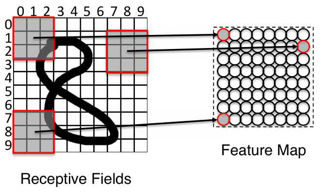
For example, imagine we wish to train a network to identify digits in images of $10\times 10$ pixels. In this scenario we may design a network so that one of the neurons in the network inspects the pixels in the top-left corner of the figure to check if a visual feature is present. The image at the top of Figure 2 illustrates such a neuron. This neuron inspects the pixels $(0,0),\dots,(2,2)$ and applies the function defined by the weight vector $<w_{0},\dots,w_{8}>$ . This neuron will return a high activation if the appropriate pixel pattern is present in the pixels input to the function and low otherwise. We can now create a copy of this neuron that uses the same weights $<w_{0},\dots,w_{8}>$ but which inspects a different set of pixels in the image: the image at the bottom of Figure 2 illustrates such a neuron, this particular neuron inspects the pixels $(0,1),\dots,(2,3)$ . If the visual feature that the function defined by the weight vector $<w_{0},\dots,w_{8}>$ occurs in either of the image patches inspected by these two neurons, then one of the neurons will fire.

Extending the idea of a set of neurons with shared weights inspecting a full image results in the concept of a feature map. In a CNN a feature map consists of a group of neurons that share the same set of weights on their inputs. This means that each group of neurons that share their weights learns to identify a particular visual feature and each neuron in the group acts as a detector for that feature. In a CNN the neurons within each group are arranged so that each neuron examines a different local region in the image. The set of pixels that each neuron in the feature map inspects is known as the receptive field of that neuron. The neurons and the related receptive fields are arranged so that together the receptive fields cover the entire input image. Consequently, if the visual feature the group detects occurs anywhere in the image one of the neurons in the group will identify it. Figure 3 illustrates a feature map and how each neuron in the feature map has a different receptive field and how the neurons and fields are organised so that taken together the receptive fields of the feature map cover the entire input image. Note that the receptive fields of neighbouring neurons typically overlap. In the architecture illustrated in Figure 3 the receptive fields of neighbouring neurons will overlap by either two columns (for horizontal neighbours) or by two rows (for vertical neighbours). However, an alternative organisation would be to reduce the number of neurons in the feature map and reduce the amount of overlap in the receptive fields. For example, if the receptive fields only overlapped by one row or one column then we would only need half the number of neurons in the feature map to cover the entire input image. This would of course result in a “two-to-one under-sampling in each direction” Le Cun (1989).

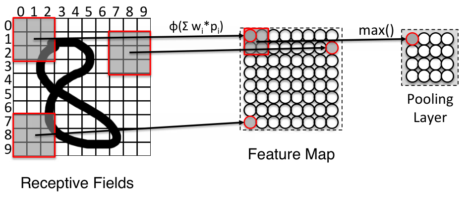
The idea of applying the same function repeatedly across an input space by defining a set of neurons where each neuron applies the function to a different part of the input is very general and can be used irrespective of the type of function being applied. CNNs networks often use the same technique to under-sample the output from a feature map. The motivation for under-sampling is to discard locational information in favour of generalising the network’s ability to identify visual features in a shift invariant manner. The standard way to implement under-sampling on the output of a feature map is to use a pooling layer, so called as it pools information from a number of neurons in a feature map. Each neuron in a pooling layer inspects the outputs of a subset of the neurons in a feature map, in a very similar way to the way the neuron in the feature map each has a receptive field in the input. Often the function used by neurons in a pooling layer is the max function. Essentially, a max pooling neuron outputs the maximum activation value of any of the neurons in the preceding layer that it inspects. Figure 4 illustrates the extension of the feature map in Figure 3 with a pooling layer. The output of the highlighted neuron in the pooling layer is simply the highest activation across the 4 neurons in the feature map that it inspects. Pooling obviously discards locational information at a local level, after pooling the network knows that a visual feature occurred in a region of the image but does not know where precisely within the region the feature occurred.

A CNN network is not restricted to only one feature map or one pooling layer. A CNN network can consist of multiple feature maps and pooling layers working in parallel where the outputs of these different streams of processing are finally merged to one or more fully connected layers (see Figure 5). Furthermore, these basic building blocks of feature maps and pooling layers can be sequenced in many different ways: the output of one feature map layer can be used as the input to another feature map layer, and the output of a pooling layer may be the input to a feature map layer. Consequently, a CNN architecture is very flexible and can be composed of multiple layers of feature maps and pooling layers. For example, a CNN could include a feature map that is fed into a pooling layer which in turn acts as the input for a second feature map layer which itself is down-sampled using another pooling layer, and so on, until the outputs of a layer are eventually fed into a fully-connected feed-forward layer where the final prediction is calculated: feature map $\rightarrow$ pooling $\rightarrow$ feature map $\rightarrow$ pooling $\rightarrow$ $dots$ $\rightarrow$ fully-connected layer. Obviously with each extra layer of pooling the network discards more and more location information.

2.2 Recurrent Neural Network Language Models

Recurrent Neural Networks (RNN)¹¹ 1 This introduction to Recurrent Neural Networks is based on Kelleher (2016). are an ideal neural network architecture for processing sequential data such as language. Generally, RNN models are created by extending a feed-forward neural network that has just one hidden layer with a memory buffer, as shown in Figure 6(a).

RNNs process sequential data one input at a time. In an RNN the outputs of the neurons in the hidden layer of the network for one input are feed back into the network as part the next input. Each time an input from a sequence is presented to the network the output from the hidden units for that input are stored in the memory buffer overwriting whatever was in the memory (Figure 6(b)). At the next time step when the next data point in the sequence is considered, the data stored in the memory buffer is merged with the input for that time step (Figure 6(c)). Consequently, as the network moves through the sequence there is a recurrent cycle of storing the state of the network and using that state at the next time step (Figure 6(d)).

(a) Adding a memory buffer to a feed-forward neural network with one hidden layer

(b) Writing the activation of the hidden layer to the memory buffer after processing the input at time

t

t+1

(d) The cycle of writing to memory and merging with the next input as the network processes a sequence

Figure 6: The flow of data between the memory buffer and the hidden layer in a recurrent neural network

In order to simplify the following figures we do not draw the individual neurons and connections but represent each layer of neurons as a rounded box and show the flow of information between layers with arrows. Also, we refer to the input layer as $x_{t}$ , the hidden layer as $h_{t}$ , the output layer as $y_{t}$ , and the memory layer as $h_{t-1}$ . Figure 7a illustrates the use of this schematic representation of layers of neurons and the flow of information through an RNN and Figure 7b shows the same network using the shorter naming convention.

(a)

(b)

Figure 7: Recurrent Neural Network (RNN)

Figure 8 demonstrates the flow of information through an RNN as it processes a sequence of inputs. An interesting thing to note is that there is a path connecting each $h$ (the hidden layer for each input) to all the previous $h$ s. Thus, the hidden layer in an RNN at each point in time is dependent on its past. In other words, the network has a memory so that when it is making a decision at time step $t$ it can remember what it has seen previously. This allows the model to take into account data that depends on previous data, for example in sequences. This is the reason why an RNN is useful for language processing: having a memory of the previous words that have been observed in a sequence of a sentence is predictive of the words that follow them.

Figure 8: An RNN unrolled in time

A language model is a computational model that takes a sequence of words as input and returns a probability distribution from which the probability of each vocabulary word being the next word in the sequence can be predicted. An RNN language model can be trained to predict the next word in a sequence. Figure 9 illustrates how information flows through an RNN language model as it processes a sequence of words and attempts to predict the next word in the sequence after each input. The * indicates the next word as predicted by the system. All going well $*Word_{2}=Word_{2}$ but if the system makes a mistake this will not be the case.

Figure 9: RNN language model unrolled in time

When we have trained a language model we can make it to “hallucinate” or generate language by giving it an initial word and then inputting the word that the language model predicts as the most likely next word as the following input word into the model, etc. Figure 10 shows how we can use an RNN language model to generate text by feeding the words the language model predicts back into the model.

Figure 10: Using an RNN language model to generate a word sequence

3 Grounding Spatial Language in Perception

The symbol grounding problem is the problem of how the meaning of a symbol can be grounded in anything other than other meaningless symbols. Harnad (1990) argues the symbolic representations must be grounded bottom-up from two forms of non-symbolic sensor representations: iconic representations which can be understood as sensory experience of objects and events, and categorial representations which are feature detectors that are triggered by invariant features of objects and events within these sensory experiences. Given these two foundational non-symbolic representations, a grounded symbolic system can be built up with the elementary symbols of this system being the symbolic names or labels of the object and event categories that are distinguished within the categorical representations of the agent. Essentially, the meaning of an elementary symbol is the categorisation of sensor grounded experience.

The description “meaningless” in the definition above (originally made by Harnad (1990)) should be discussed in relation to the work in distributional semantics Turney et al. (2010) which has been used very successfully for computational representation of meaning. The reason why distributional semantic representations work is that word contexts capture indirectly latent situations that co-occuring words are all referring to. Distributional semantic models are built from grounded language (which is therefore not “meaningless”) it is only that grounded representations are not included in the model. Grounding is expressed indirectly through word co-occurrences.

Roy (2005) extends Harnad’s approach by setting out a framework of semiotic schemas that ground symbolic meaning in a causal-predictive cycle of action and perception. Within Roy’s framework meaning is ultimately grounded in schemas where each schema is a belief network that connects action, perception, attention, categorisation, inference, and prediction. These schemas can be understood as the interface between the external world (reached through the action and perception components of the schemas) and the agents internal cognitive processes (attention, categorisation, inference, and prediction).

Spatial language is an interesting case study in grounding language in perception because linguistic descriptions of perceived spatial relations between objects are intrinsically about the world and as such should be grounded within an agent’s perception of that world Dobnik (2009); Kelleher and Costello (2009). The most common form of spatial language discussed in the literature is a locative expression. A locative expression is composed of a noun phrase modified by a prepositional phrase that specifies the location of the referent of the noun phrase relative to another object. We will use the word target object to refer to the object whose position is being described and the term landmark object to refer to the object that the target object’s location is described relative to²² 2 The literature on locative expressions uses uses a variety of terms to describe the target and the landmark objects, for a review see Kelleher (2003); Dobnik (2009). Other terms found in the literature for the target object include: trajector, local object, and figure object. Other terms used to describe the landmark object include: reference object, relatum, and ground., the annotations on the following example locative expression illustrates this terminology:

$\underbrace{\underbrace{\underbrace{The~big~red~book}_{Target}~\underbrace{on~\underbrace{the~table}_{Landmark}}_{\begin{subarray}{c}Prepositional\\ Phrase\end{subarray}}}_{Noun~Phrase}}_{Locative~Expression}$

Previous work on spatial language has revealed a range of factors that impinge on the interpretation of locative expressions. An obvious component in the grounding of a spatial description is the scene geometry and the size and shape of region described by the spatial term within that geometry. The concept of a spatial template is used to describe these regions and several experiments have revealed how these templates vary across spatial terms and languages, e.g., Logan and Sadler (1996); Kelleher and Costello (2005); Dobnik and Åstbom (2017).

It has also been shown that the geometry of a spatial template for a given preposition is affected by a number cognitive and contextual factors, including:

•

perceptual attention Regier and Carlson (2001); Burigo and Knoeferle (2015); Kluth and Schultheis (2014),
•

the viewer’s perspective on the landmark(s) Kelleher and van Genabith (2006),
•

object occlusion Kelleher et al. (2011),
•

frame of reference ambiguity and alignment between the landmark object and reference frames Carlson-Radvansky and Logan (1997); Burigo and Coventry (2004); Kelleher and Costello (2005),
•

the location of other distractor objects in the scene Kelleher and Kruijff (2005b); Costello and Kelleher (2006); Kelleher et al. (2006),
•

and the richness of the perceptual context Dobnik and Åstbom (2017).

The last point is related to the fact that factors affecting semantics of spatial descriptions go beyond scene geometry and include the functional relationships between the target and the landmark Coventry (1998); Coventry et al. (2001); Coventry and Garrod (2004) and force dynamics within the scene Coventry et al. (2005); Sjöö (2011). These functional relations can be captured as meanings induced from word distributions Dobnik and Kelleher (2013); Dobnik and Kelleher (2014). Another important factor of (projective) spatial descriptions is their contextual underspecification in terms of the assigned frame of reference which is coordinated through dialogue interaction between conversational participants Dobnik et al. (2015). It is therefore based on their coordinated intentions in their interaction.

The research in spatial language semantics highlights its multifaceted nature. Spatial language draws upon (i) geometric concepts, (ii) world knowledge (i.e., an understanding of functional relationships and force dynamics), and (iii) perceptual and discourse cues. Thus in order for a computational system to adequately model spatial language semantics it should accommodate all or most of these factors.

4 Spatial Language in DL

The question that this paper addresses is whether deep learning image captioning architectures as currently constituted are capable of grounding spatial language within the images they are captioning. The outputs of these systems are impressive and often include spatial descriptions. Figure 1 (based on an example from Xu et al. (2015)) provides an indicative example of the performance of these systems. The generated caption in this case is accurate and what is particularly interesting is that it includes a spatial description: over water. Indeed, the vast majority of generated captions listed in Xu et al. (2015) include spatial descriptions, some of which include:³³ 3 The emphasis on the spatial descriptions were added here.

•

“A woman is throwing a frisbee in a park”
•

“A dog is standing on a hardwood floor”
•

“A group of people sitting on a boat in the water”.

The fact that these example captions include spatial descriptions and that the captions are often correct descriptions of the input image begs the question of whether image captioning systems are actually learning to ground the semantics of these spatial terms in the images. The nature of neural network systems makes it difficult to directly analyse what a system is learning, however there are a number of reasons why it would be surprising to find that these systems were grounding spatial language. First, recall from the review of grounding in Section 3 that spatial language draws on a variety of information, including:

•

scene geometry,
•

perceptual cues such as object occlusion,
•

world knowledge including functional relationships and force dynamics,
•

and coordinated intentions of interacting agents.

Considering only scene geometry, these image captioning systems use CNNs to encode the representation of the input image. Recall from Section 2.1 that CNNs discard locational information through the (down-sampling) pooling mechanism and that such down-sampling may be applied several times within a CNN pipeline. Although it is possible that the encoding generated by a CNN may capture rough relative positions of objects within a scene, it is likely that this encoding is too rough to accommodate the level of sensitivity of spatial descriptions to location that experimental studies of spatial language have found to be relevant (cf. the changes in acceptability ratings in Logan and Sadler (1996); Kelleher and Costello (2005); Dobnik and Åstbom (2017) as a target object moved position relative to the landmark). The architecture of CNNs also points to the fact that these systems are unlikely to be modelling perceptual cues. CNNs essentially work by identifying what an object is through a hierarchical merging of local visual features that are predictive of the object type. These local visual features are likely to be features that are parts of the object and therefore frequently co-occur with the object label. Consequently, CNNs are unlikely to learn to identify an object type via context and viewpoint dependent cues such as occlusion. Finally, neither a CNN nor an RNN as currently used in the image description tasks provide mechanisms to learn force-dynamics or functional relationships between objects (cf. Coventry et al. (2005); Battaglia et al. (2013)) nor do they take into account agent interaction. Viewed in this light the current image captioning systems appear to be missing most of the key factors necessary to ground spatial language. And, yet they do appear to generate reasonably accurate captions that include spatial descriptions.

There are a number of factors that may be contributing to this apparent ability. First, an inspection of the spatial descriptions used in the generated captions reveals that they tend to include topological rather than projective spatial prepositions (e.g., on and in rather than to the left of and above): in a forest, in a park, in a field, in the field with trees, in the background, on a bed, on a road, on a skateboard, at a table. These spatial descriptions are more underspecified with regard to the location of the target object relative to the landmark object than projective descriptions which also require grounding of direction within a frame of reference. Topological descriptions are semantically adequate already if the target is just proximal to the landmark and hence it is more likely that a caption will be acceptable. Furthermore, it is frequently the case that given a particular label for a landmark it is possible to guess the appropriate preposition irrespective of the image and/or the target object type or location. Essentially the task posed to these systems is to fill the blanks with one of at, on, in:

•

TARGET a field,
•

TARGET the background,
•

TARGET a road,
•

TARGET a table.

Although the system may get some of the blanks wrong it is likely to get many of them right. This is because the system can use distributional knowledge of words which captures some grounding indirectly as discussed in Section 3. Indeed, recent research has shown that co-occurrence of nouns with a preposition within a corpus of spatial descriptions can reveal functional relations between objects referred to by the nouns Dobnik and Kelleher (2013); Dobnik and Kelleher (2014). Word co-occurrence is thus highly predictive of the correct preposition. Consequently, language models trained on image description corpora indirectly model partially grounded functional relations, at least within the scope of the co-occurrence likelihood of prepositions and nouns.

The implication of this is that current image captioning systems do not ground spatial descriptions in the images they take as input. Instead, the apparent ability of these systems to frequently correctly use spatial prepositions to describe spatial relations within the image is the result of the RNN language model learning to predict the most likely preposition to be used given the target and landmark nouns where these nouns are predicted from the image by the CNN.

There is a negative and a positive side to this conclusion. Let’s start with the negative side. The distinction between cognitive representations of what something is versus where something is has a long tradition in spatial language and spatial cognition research Landau and Jackendoff (1993). These image captioning systems would appear to be learning representations that allow them to ground the semantics of what. But they are not learning representations that enable them to ground the semantics of where. Instead, they rely on the RNN language model to make good guesses of the appropriate spatial terms to use based on word distributions. The latter point introduces the positive side. It is surprising how much and how robustly semantic information can be captured by distributional language models. Of course, language models cannot capture the geometric relations between objects, for example they are not able to distinguish successfully the difference in semantics between the chair is to the left of the table and the chair is to the right of the table as left and right would occur in exactly the same word contexts. However, as we argued in Section 3 spatial language is not only spatial but also affected by other sources of knowledge that leave an imprint in the word distributions which capture relations between higher-level categorical representations built upon the elementary grounded symbols Harnad (1990). It follows that some categorical representations will be closer to and therefore more grounded in elementary symbols, something that has been shown for spatial language Coventry (1998); Coventry et al. (2001); Coventry and Garrod (2004); Dobnik and Kelleher (2013); Dobnik and Kelleher (2014). In conclusion, it follows that successful computational models of spatial language require both kinds of knowledge.

5 Conclusions

In this paper we examined the current architecture for generating image captions with deep learning and argued that in its present setup they fail to ground the meaning of spatial descriptions in the image but nonetheless achieve a good performance in generating spatial language which is surprising given the constraints of the architecture that they are working with. The information that they are using to generate spatial descriptions is not spatial but distributional, based on word co-occurrence in a sequence as captured by a language model. While such information is required to successfully predict spatial language, it is not sufficient. We see at least two useful areas of future work. On one hand, it should be possible to extend the deep learning configurations for image description to take into account and specialise to learn geometric representations of objects, just as the current deep learning configurations are specialised to learn visual features that are indicative of objects. The work on modularity of neural networks such as Andreas et al. (2016); Johnson et al. (2017) may be relevant in this respect. On the other hand, we want to study how much information can be squeezed out of language models to successfully model spatial language and what kind of language models can be built to do so.

Acknowledgements

The research of Kelleher was supported by the ADAPT Research Centre. The ADAPT Centre for Digital Content Technology is funded under the SFI Research Centres Programme (Grant 13/RC/2106) and is co-funded under the European Regional Development Funds.

The research of Dobnik was supported by a grant from the Swedish Research Council (VR project 2014-39) for the establishment of the Centre for Linguistic Theory and Studies in Probability (CLASP) at Department of Philosophy, Linguistics and Theory of Science (FLoV), University of Gothenburg.

References

Andreas et al. (2016) Jacob Andreas, Marcus Rohrbach, Trevor Darrell, and Dan Klein. 2016. Learning to compose neural networks for question answering. CoRR abs/1601.01705:1–10.
Battaglia et al. (2013) Peter W. Battaglia, Jessica B. Hamrick, and Joshua B. Tenenbaum. 2013. Simulation as an engine of physical scene understanding. Proceedings of the National Academy of Sciences 110(45):18327–18332.
Brenner et al. (2007) Michael Brenner, Nick Hawes, John D. Kelleher, and Jeremy L. Wyatt. 2007. Mediating between qualitative and quantitative representations for task-orientated human-robot interaction. In Proceedings of the International Joint Conference on Artificial Intelligence (IJCAI). AAAI, pages 2072–2077.
Burigo and Coventry (2004) Michele Burigo and Kenny Coventry. 2004. Reference frame conflict in assigning direction to space. In International Conference on Spatial Cognition. Springer, pages 111–123.
Burigo and Knoeferle (2015) Michele Burigo and Pia Knoeferle. 2015. Visual attention during spatial language comprehension. PloS one 10(1):e0115758.
Carlson-Radvansky and Logan (1997) L.A. Carlson-Radvansky and G.D. Logan. 1997. The influence of reference frame selection on spatial template construction. Journal of Memory and Language 37:411–437.
Costello and Kelleher (2006) Fintan Costello and John D. Kelleher. 2006. Spatial prepositions in context: The semantics of Near in the presense of distractor objects. In Proceedings of the 3rd ACL-Sigsem Workshop on Prepositions. pages 1–8.
Coventry et al. (2005) Kenny R. Coventry, Angelo Cangelosi, Rohanna Rajapakse, Alison Bacon, Stephen Newstead, Dan Joyce, and Lynn V. Richards. 2005. Spatial prepositions and vague quantifiers: Implementing the functional geometric framework. In Christian Freksa, Markus Knauff, Bernd Krieg-Brückner, Bernhard Nebel, and Thomas Barkowsky, editors, Spatial Cognition IV. Reasoning, Action, Interaction, Springer Berlin Heidelberg, volume 3343 of Lecture Notes in Computer Science, pages 98–110.
Coventry et al. (2001) Kenny R. Coventry, Mercè Prat-Sala, and Lynn Richards. 2001. The interplay between geometry and function in the apprehension of Over, Under, Above and Below. Journal of Memory and Language 44(3):376–398.
Coventry (1998) K.R. Coventry. 1998. Spatial prepositions, functional relations, and lexical specification. In P. Olivier and K.P. Gapp, editors, Representation and Processing of Spatial Expressions, Lawrence Erlbaum Associates, pages 247–262.
Coventry and Garrod (2004) K.R. Coventry and S. Garrod. 2004. Saying, Seeing and Acting. The Psychological Semantics of Spatial Prepositions. Essays in Cognitive Psychology Series. Lawrence Erlbaum Associates.
Dobnik (2009) Simon Dobnik. 2009. Teaching mobile robots to use spatial words. Ph.D. thesis, University of Oxford: Faculty of Linguistics, Philology and Phonetics and The Queen’s College, Oxford, United Kingdom. 289 pages. http://www.dobnik.net/simon/documents/thesis.pdf.
Dobnik and Åstbom (2017) Simon Dobnik and Amelie Åstbom. 2017. (Perceptual) grounding as interaction. In Volha Petukhova and Ye Tian, editors, Proceedings of Saardial – Semdial 2017: The 21st Workshop on the Semantics and Pragmatics of Dialogue. Saarbrücken, Germany, pages 17–26.
Dobnik et al. (2015) Simon Dobnik, Christine Howes, and John D. Kelleher. 2015. Changing perspective: Local alignment of reference frames in dialogue. In Christine Howes and Staffan Larsson, editors, Proceedings of goDIAL – Semdial 2015: The 19th Workshop on the Semantics and Pragmatics of Dialogue. Gothenburg, Sweden, pages 24–32.
Dobnik and Kelleher (2013) Simon Dobnik and John D. Kelleher. 2013. Towards an automatic identification of functional and geometric spatial prepositions. In Proceedings of PRE-CogSsci 2013: Production of referring expressions – bridging the gap between cognitive and computational approaches to reference. Berlin, Germany, pages 1–6.
Dobnik and Kelleher (2014) Simon Dobnik and John D Kelleher. 2014. Exploration of functional semantics of prepositions from corpora of descriptions of visual scenes. In Anja Belz, Marie-Francine Moens, and Alan F. Smeaton, editors, Proceedings of the 1st Technical Meeting of the European Network on Integrated Vision and Language (V&L Net) a Workshop at the 25th International Conference on Computational Linguistics (COLING). Association of Computational Lingustics, Dublin, Ireland, pages 33–37.
Dobnik and Kelleher (2016) Simon Dobnik and John D. Kelleher. 2016. A model for attention-driven judgements in type theory with records. In Julie Hunter, Mandy Simons, and Matthew Stone, editors, JerSem: The 20th Workshop on the Semantics and Pragmatics of Dialogue. New Brunswick, NJ USA, volume 20, pages 25–34.
Gorniak and Roy (2004) Peter Gorniak and Deb Roy. 2004. Grounded semantic composition for visual scenes. Journal of Artificial Intelligence Research 21:429–470.
Harnad (1990) Stevan Harnad. 1990. The symbol grounding problem. Physica D 42:335–346.
Hochreiter and Schmidhuber (1997) Sepp Hochreiter and Jürgen Schmidhuber. 1997. Long short-term memory. Neural Computation 9(8):1735–1780.
Johnson et al. (2017) Justin Johnson, Bharath Hariharan, Laurens van der Maaten, Judy Hoffman, Fei-Fei Li, C. Lawrence Zitnick, and Ross B. Girshick. 2017. Inferring and executing programs for visual reasoning. CoRR abs/1705.03633(n):n.
Kelleher (2003) John D. Kelleher. 2003. A Perceptually Based Computational Framework for the Interpretation of Spatial Language. Ph.D. thesis, Dublin City University.
Kelleher (2016) John D. Kelleher. 2016. Fundamentals of machine learning for neural machine translation. In Proceedings of the Translating Europen Forum 2016: Focusing on Translation Technologies (doi:10.21427/D78012). European Commission Directorate-General for Translation.
Kelleher and Costello (2005) John D. Kelleher and Fintan Costello. 2005. Cognitive representations of projective prepositions. In Proceedings of the Second ACL-Sigsem Workshop of The Linguistic Dimensions of Prepositions and their Use in Computational Linguistic Formalisms and Applications..
Kelleher and Costello (2009) John D. Kelleher and Fintan J. Costello. 2009. Applying computational models of spatial prepositions to visually situated dialog. Computational Linguistics 35(2):271–306.
Kelleher and Kruijff (2005a) John D. Kelleher and Geert-Jan M. Kruijff. 2005a. A context-dependent algorithm for generating locative expressions in physically situated environments. In Proceedings of the Tenth European Workshop on Natural Language Generation (ENLG-05).
Kelleher and Kruijff (2005b) John D. Kelleher and Geert-Jan M. Kruijff. 2005b. A context-dependent model of proximity in physically situated environments. In Proceedings of the 2nd ACL-SIGSEM Workshop on The Linguistic Dimensions of Prepositions and their Use in Computational Linguistics Formalisms and Applications, Colchester, UK.
Kelleher et al. (2006) John D. Kelleher, Geert-Jan M. Kruijff, and Fintan Costello. 2006. Proximity in context: an empricially grounded computation model of proximity for processing topological spatial expressions. In Proceedings ACL/Coling 2006. Sydney, Australia.
Kelleher et al. (2011) John D. Kelleher, Robert J. Ross, Colm Sloan, and Brian Mac Namee. 2011. The effect of occlusion on the semantics of projective spatial terms: A case study in grounding language in perception. Cognitive Processing 12(1):95–108.
Kelleher and van Genabith (2006) John D. Kelleher and Josef van Genabith. 2006. A computational model of the referential semantics of projective prepositions. In P. Saint-Dizier, editor, Syntax and Semantics of Prepositions, Kluwer Academic Publishers, Dordrecht, The Netherlands, Speech and Language Processing.
Kluth and Schultheis (2014) Thomas Kluth and Holger Schultheis. 2014. Attentional distribution and spatial language. In International Conference on Spatial Cognition. Springer, pages 76–91.
Landau and Jackendoff (1993) Barbara Landau and Ray Jackendoff. 1993. ”What” and ”where” in spatial language and spatial cognition. Behavioral and Brain Sciences 16:217–265.
Le Cun (1989) Yann Le Cun. 1989. Generalization and network design strategies. Technical Report CRG-TR-89-4, University of Tronoto Connectionist Research Group.
Lecun et al. (1998) Y. Lecun, L. Bottou, Y. Bengio, and P. Haffner. 1998. Gradient-based learning applied to document recognition. Proceedings of the IEEE 86(11):2278–2324.
LeCun et al. (2015) Yann LeCun, Yoshua Bengio, and Geoffrey Hinton. 2015. Deep learning. Nature 521(7553):436–444.
Lee et al. (2009) Honglak Lee, Roger Grosse, Rajesh Ranganath, and Andrew Y. Ng. 2009. Convolutional deep belief networks for scalable unsupervised learning of hierarchical representations. In Proceedings of the 26th Annual International Conference on Machine Learning. ACM, New York, NY, USA, ICML ’09, pages 609–616.
Logan and Sadler (1996) G.D. Logan and D.D. Sadler. 1996. A computational analysis of the apprehension of spatial relations. In M. Bloom, P.and Peterson, L. Nadell, and M. Garrett, editors, Language and Space, MIT Press, pages 493–529.
McKevitt (1995) P. McKevitt, editor. 1995. Integration of Natural Language and Vision Processing (Vols. I-IV). Kluwer Academic Publishers, Dordrecht, The Netherlands.
Regier and Carlson (2001) T Regier and L. Carlson. 2001. Grounding spatial language in perception: An empirical and computational investigation. Journal of Experimental Psychology: General 130(2):273–298.
Roy (2005) Deb Roy. 2005. Semiotic schemas: A framework for grounding language in action and perception. Artificial Intelligence 167(1-2):170–205.
Schmidhuber (2015) Jürgen Schmidhuber. 2015. Deep learning in neural networks: An overview. Neural Networks 61:85 – 117.
Schütte et al. (2017) Niels Schütte, Brian Mac Namee, and John D. Kelleher. 2017. Robot perception errors and human resolution strategies in situated human–robot dialogue. Advanced Robotics 31(5):243–257.
Sjöö (2011) Kristoffer Sjöö. 2011. Functional understanding of space: Representing spatial knowledge using concepts grounded in an agent’s purpose. Ph.D. thesis, KTH, Computer Vision and Active Perception (CVAP), Centre for Autonomous Systems (CAS), Stockholm, Sweden.
Sutskever et al. (2014) Ilya Sutskever, Oriol Vinyals, and Quoc V Le. 2014. Sequence to sequence learning with neural networks. In Advances in neural information processing systems. pages 3104–3112.
Tellex (2010) Stefanie Tellex. 2010. Natural language and spatial reasoning. Ph.D. thesis, Massachusetts Institute of Technology.
Turney et al. (2010) Peter D Turney, Patrick Pantel, et al. 2010. From frequency to meaning: Vector space models of semantics. Journal of artificial intelligence research 37(1):141–188.
Winograd (1973) T. Winograd. 1973. A procedural model of language understanding. In R.C. Schank and K.M. Colby, editors, Computer Models of Thought and Language, W. H. Freeman and Company, pages 152–186.
Xu et al. (2015) Kelvin Xu, Jimmy Ba, Ryan Kiros, Kyunghyun Cho, Aaron Courville, Ruslan Salakhudinov, Rich Zemel, and Yoshua Bengio. 2015. Show, attend and tell: Neural image caption generation with visual attention. In International Conference on Machine Learning. pages 2048–2057.