Study on the mapping of halo clustering from real space to redshift space

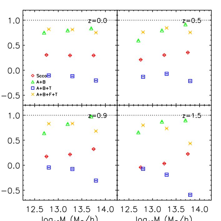
The measurements of real space power spectra and higher order polynomials in eq. (8) require the sampling of volume-weighted halo velocity field. However, halos are sparsely and inhomogeneously distributed, thus the sampled velocity field is severely contaminated by the sampling artifact even at the linear scales of $k\sim 0.1\,h\,{\rm Mpc}^{-1}$ [114, 115]. As shown in eq. (23), [105] developed a novel strategy to overcome this sampling artifact problem and proposed an accurate fitting formula for $b_{v}(k,z)$ at $k\leqslant 0.25\,h\,{\rm Mpc}^{-1}$. We estimate the halo velocity bias by substituting the linear halo density biases in Table 2 to eq. (23). Figure 1 shows the calculated velocity biases. In figure 1, curves with different colors and line-styles represent $b_{v}$ of different halo mass bins, and from top to bottom, lines correspond to $b_{v}$ calculations at $z=(0.0,\,0.5,\,0.9,\,1.5)$ respectively. Most of the estimated velocity biases have no bigger than $1\%$ deviation from unity at $k\lesssim 0.2\,h\,{\rm Mpc}^{-1}$. Thus it is safe to set $b_{v}=1$ for theoretical calculations of $P_{\delta_{h}\theta_{h}}$ and $P_{\theta_{h}\theta_{h}}$ in eq. (8) hereafter.

However, the effect of $b_{v}$ on higher order terms is a bit more complicated. Higher order terms are expressed as integrals of power spectra, bispectra, trispectra, etc. The integration interval includes small scales of $k>0.2\,h\,{\rm Mpc}^{-1}$, where the halo velocity bias could significantly deviate from unity. To this point, it is not straightforward to predict the actual influence of halo velocity bias on RSD effect. To overcome this complexity, we construct an estimator, analogous to the estimator for studying the multi-streaming effect in [120], that is

in which

In this estimator, $P_{h,v_{DM}}^{\rm(S)}(k,\mu)$ is evaluated by substituting the sampled halo density field and dark matter velocity field into eq. (25). Referring to eq. (2), it is easy to find that $A_{b_{v}}$ fully quantifies the influence of halo velocity bias on the RSD effect, except that the small scale (smaller than grid size) dark matter velocity dispersion is omitted in calculating $P_{h,v_{DM}}^{\rm(S)}(k,\mu)$. In [120], this grid effect is used to study the multi-streaming effect of dark matter RSD, while for the halo case here, since halo velocity averages over the dark matter velocity inside a halo, the multi-streaming effect is already very much suppressed in $P_{h,v_{DM}}^{\rm(S)}(k,\mu)$. Therefore, under the assumption of negligible multi-streaming effect, we consider $A_{b_{v}}$ as a robust estimator in quantifying the systematic effect of halo velocity bias, and the results are shown in figure 2.

In general, for the halo mass bins whose velocity biases are lower than unity, we see that $A_{b_{v}}$ is greater than 1, indicating that $P_{h}^{\rm(S)}$ is less damped than that induced by dark matter velocity field. The systematic error, as quantified by $A_{b_{v}}$, could be as large as $10\%$ for large halos at $k\mu=0.2\,h\,{\rm Mpc}^{-1}$. Figure 2 falsifies the usual assumption that we could represent halo velocity field by dark matter velocity field. Furthermore, $A_{b_{v}}$ is not a pure function of $k\mu$. It shows obvious $k$ and $\mu$ dependence separately. The detailed modelling of $A_{b_{v}}$ is beyond this paper’s scope. We will assume $A_{b_{v}}$ is a only function of $k\mu$ and approximate it with three FoG functional forms.

The fitted $\alpha^{\rm velb}_{z,h}$ is shown on the top left corner of each panel.

Since $A_{b_{v}}$ fully quantifies the halo velocity bias effect, from now on we replace $\theta_{h}$ with $\theta$, the volume–weighted dark matter velocity fields. The dark matter velocity fields are computed by the nearest particle method (NP method) [89]. In other words, the velocity of the nearest dark matter particle to each grid is assigned to this grid for computing $\theta$. The dark matter particles have much higher number density than that of halos. The sampling artifact is controlled to be less than $1\%$ in our simulations at $k\leqslant 0.2\,h\,{\rm Mpc}^{-1}$ [120]. In practice, $P_{\delta_{h}\theta_{h}}$ and $P_{\theta_{h}\theta_{h}}$ are replaced by $P_{\delta_{h}\theta}$ and $P_{\theta\theta}$ in our test. The same treatment is applied to higher order polynomial measurements, which are computed by combining fields such as of $u_{z}(\mbox{\boldmath$r$})$, $\nabla_{z}u_{z}(\mbox{\boldmath$r$})$, $\delta_{h}u_{z}(\mbox{\boldmath$r$})$ and $u_{z}\nabla_{z}u_{z}(\mbox{\boldmath$r$})$. The detailed methodology of higher order polynomial calculation is explained in [96] with dark matter particles as an example. The key strategy is that we compute these various field combinations in the configuration space, and transform them into the Fourier space, where we complete all two–point statistical measurements and derive $P_{{\rm perturbed},h}$. With the measured $P_{h}^{\rm(S)}(k,\mu)$ and $P_{{\rm perturbed},h}$ on hand, we could test the accuracy of eq. (8) by fitting the FoG term through the least-$\chi^{2}$ method. The fitting range of $k$ is chosen to be $0.035-0.205\,h\,{\rm Mpc}^{-1}$, with bin size $\Delta k=0.01\,h\,{\rm Mpc}^{-1}$.

As pointed out in [88, 96], the FoG term is an exponential function whose index contains indefinite orders of terms to be formulated in the closed form. It was verified in [89, 96] that this FoG term could be effectively formulated with a simple Gaussian function, as the leading order term dominates in our interesting range of scales. It was also verified in [89] that the bulk flow component of peculiar velocity field dominates the FoG term, and figure 1 indicates that halo and dark matter have similar bulk flow components. Hence we expect the Gaussian function will still be a good FoG approximation, which is proved in figure 3.

In our test, we define $D^{\rm FoG}_{\rm res}$, the measured residual FoG term, as $P_{h}^{\rm(S)}(k,\mu)/P_{{\rm perturbed},h}$. If the perturbed term $P_{{\rm perturbed},h}$ is correctly estimated, the residual FoG will be well represented by the single Gaussian function in terms of $k\mu$, regardless of different $k$. Figure 3 shows the fractional difference between the measured $P_{h}^{\rm(S)}$ and our model with Gaussian FoG function for three halo mass bins at 4 redshifts. It is effectively the fractional difference between $D^{\rm FoG}_{\rm res}$ and the best fitted Gaussian FoG function. Our RSD mapping formula is proven to be accurate within $1\sim 2\%$ at $k\lesssim 0.2\,h\,{\rm Mpc}^{-1}$, depending on halo bins with different masses and redshifts. In addition, we compare the best fitted Lorentzian FoG model (dashed line) and Lorentzian2 FoG model (dot-dashed line) with the best fitted Gaussian model. The corresponding reduced $\chi^{2}$/dof and best fitted velocity dispersion $\sigma^{2}_{z,h}$ of three FoG forms listed in each panel. With different best fitted $\sigma^{2}_{z,h}$ three FoG functions do not show much difference and Gaussian function is verified to be a good FoG approximation.

We further compare the effects of different higher order term combinations in our model in figure 4. We present the various combinations of higher order polynomials from the left to the right. “Scoccimarro” denotes the model proposed in [70] where no higher order polynomials are considered, as $P_{{\rm perturbed},h}=P_{\delta_{h}\delta_{h}}+2\mu^{2}P_{\delta_{h}\theta_{h}}+\mu^{4}P_{\theta_{h}\theta_{h}}$. It certainly unfits to the measurements. Conventionally, only $A+B$ combinations are adapted for most RSD data analysis, which shows the good fit only at $k\lesssim 0.1\,h\,{\rm Mpc}^{-1}$. When all combinations of $A_{h}+B_{h}+F_{h}+T_{h}$ are used, the fitting has the lowest $\chi^{2}$/dof and the residual deviates from the simple Gaussian function within $1\sim 2\%$ accuracy at $k\lesssim 0.2\,h\,{\rm Mpc}^{-1}$.

In eq. (24), we define an estimator, $A_{v_{b}}$, which fully quantifies the systematic from the halo velocity bias. Therefore, the redshift space 2D halo density power spectrum, $P_{h}^{\rm(S)}$, could be expressed as

Here we describe $A_{b_{v}}$ by a Gaussian function as an example, which is supported by figure 2. In figure 2 it also shows that $A_{b_{v}}$ could be either higher or lower than unity, meaning that $\alpha^{\rm velb}_{z,h}$ could be either negative or positive. The full understanding of $A_{b_{v}}$ calls for understanding how halo velocity bias plays its role in RSD effect, and we would like to address this issue in the future.

We go on the analyze $P_{h,v_{\rm DM}}^{\rm(S)}(k,\mu)$. It is now fully constructed by dark matter velocity field, and its FoG effect is naturally controlled by the dark matter velocity dispersion.

As a result, the fitted velocity dispersion, $\sigma_{z,h}^{2}$, has two components, $\sigma_{z,h}^{2}=\alpha^{\rm velb}_{z,h}+\sigma^{2}_{\rm DM}$. It is $\sigma^{2}_{z}=\sigma_{z,h}^{2}-\alpha^{\rm DM}_{z,h}$ which will be fairly compared to the measured dark matter velocity dispersion in figure 5.

The ratios of $\sigma^{2}_{z}$ and $\sigma^{2}_{z,\rm DM}$ are shown in figure 5. Different colors and symbols represent different combinations of higher order terms. All ratios are all below unity, in particular, $A+B+T$ model results in a negative $\sigma^{2}_{z}$ and invalidates it as a robust RSD model. $\sigma^{2}_{z}/\sigma^{2}_{z,\rm DM}\approx 1$ is expected if the expansion in terms of $j_{1}$ converges and the convergence will possibly be improved if we include higher order of $j_{1}$ terms, e.g. $j_{1}^{3}$ and $j_{1}^{4}$ terms. The results will be published in a companion paper.

We have halos with limited number density, which undergo through nonlinear evolution and have discrete and stochastic distribution. The resultant shot noise or stochastic influence needs to be controlled. For a more precise test, this uncertainty due to the stochastic term needs to be removed from the measured halo density fields.

If halos are distributed by Poisson process, the shot noise term is a constant, simply given by the inverse of halo number density, $1/\bar{n}_{h}$. However in reality, the measured shot noise at large scales exhibits the scale dependence due to the halo exclusion and nonlinear enhancement of clustering outside the exclusion scale [121]. This scale dependent shot noise term should be taken into account in our test.

First we describe the way to calculate the stochastic term. The measured halo density fluctuations $\tilde{\delta}_{h}(\mbox{\boldmath$k$})$ can be decomposed into two components, the determinent halo density fluctuations $\delta_{h}(\mbox{\boldmath$k$})$ and the stochastic uncertainty $\epsilon(\mbox{\boldmath$k$})$ [122, 123],

By definition, the dark matter density fluctuations $\delta(\mbox{\boldmath$k$})$ does not correlate with the halo stochastic noise field $\epsilon(\mbox{\boldmath$k$})$, $<\epsilon(\mbox{\boldmath$k$})\delta^{\ast}(\mbox{\boldmath$k$})>=0$. Here $b(k)$ is the deterministic halo density bias, and it can be measured by

The measured halo density bias $b(k)$ are plotted as data points in the left panel of Fig. 6. The error bars are estimated by 100 realizations of simulations. Generally it shows that, the bias becomes more non-linear, and its scale dependence becomes larger with increasing redshift and halo mass.

Next, the stochastic power spectrum $P_{\epsilon\epsilon}$ can be calculated by

We compare the measurement of $P_{\epsilon\epsilon}$ with $1/\bar{n}_{h}$ of Poisson shot noise power spectrum in the right panel of Fig. 6. The measured stochastic terms show visible scale dependence even at linear scales. The scale dependent variation of $P_{\epsilon\epsilon}$ could reach $10\%$ in some cases, invalidating a constant parametrization for $P_{\epsilon\epsilon}$. Meanwhile, the $P_{\epsilon\epsilon}$ amplitudes of two halo mass bins show opposite trends. From $z=0.0$ to $z=1.5$, that of heavy bin increases from sub-Poissonian to super-Poissonian while that of light bin decreases from super-Poissonian to sub-Poissonian. Furthermore, both evolving trends are not purely monotonic.

Compared to a Poisson random point field, halo distribution consists of two extra properties, the halo exclusion and nonlinear clustering enhancement outside the exclusion scale [121]. On one hand, halos have finite sizes. Within its radius, it is forbidden to randomly sample another halo from the dark matter density field. This halo exclusion breaks the Poisson assumption and causes a sub-Poissonian shot noise term. On the other hand, the nonlinear enhancement of clustering outside the exclusion scale will lead to a positive stochasticity correction of $P_{\epsilon\epsilon}$. The competition of these two factors results in the complicated $P_{\epsilon\epsilon}$ behavior as shown in figure 6.

In our RSD model test, we will directly use the measured shot noise term for the fitting. The modelling of this stochastic term is beyond the scope of this paper. In realistic galaxy RSD analysis, the shot noise could be dramatically reduced by weighting halos with different masses [122] or robustly modelled by proper fitting formula (e.g. [121, 124, 125, 126]).

In this subsection, the accuracy of halo density bias model is tested in detail. The velocity bias keeps to be set $b_{v}=1$, and halo density fields are described by the model. Thus the cross–power spectrum $P_{\delta_{h}\theta_{h}}(k)$ is given by,

where eq. (16) is applied. For the auto–power spectrum $P_{\delta_{h}\delta_{h}}$, we substitute eq. (17) into eq. (18), which leads to,

To be emphasized, here we are effectively modelling the cross–power spectrum $P_{\delta_{h}\delta}$, not directly the auto–power spectrum. We directly measure the $P_{\delta\theta}$ and $P_{\delta\delta}$ from simulations, and evaluate other power spectra in these two formulas by linear perturbation theory as described in Appendix A. Then we fit two free parameters, $b_{1}$ and $b_{2}$, to test the accuracy of eqs. (35) and (34) in figures 7 and 8 respectively. In the left panels of figures, the triangles with error bars are simulation measurements, and the dotted lines are the fitted models. The fitted $b_{1}$ and $b_{2}$ are written besides the power spectra. In the right panels of the figures, the fractional differences between the measurements and models are plotted. We see that for all halo mass bins and redshifts, the adopted halo density bias model reaches $1\%$ accuracy and its uncertainty will not be a major systematic error in our RSD model test. Furthermore, the fitted $b_{1}$ from $P_{\delta_{h}\delta_{h}}$ and $P_{\delta_{h}\theta_{h}}$ are consistent with each other, showing the consistency of the halo density bias model.

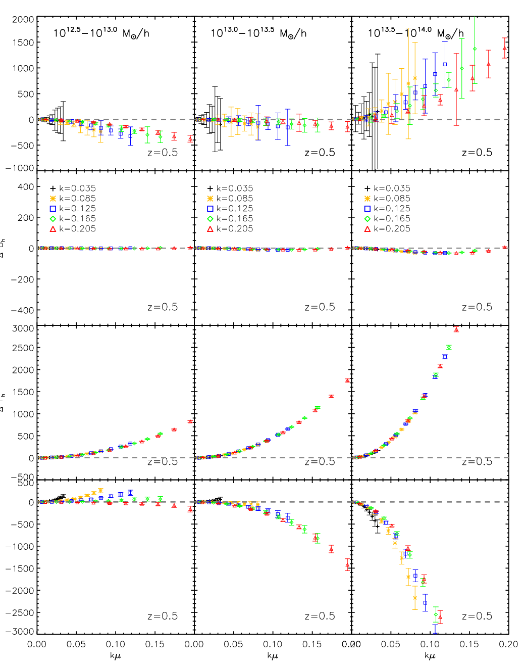
Next, the accuracy of higher order polynomial measurements under bias model are tested. It is still not clearly understood what should be the precise bias models for higher order terms, particularly for $T_{h}$, the trispectrum-related one. Considering these higher order terms are not leading contributions in comparison to $P_{\delta_{h}\delta_{h}}$, $P_{\delta_{h}\theta_{h}}$ and $P_{\theta_{h}\theta_{h}}$, we simply approximate them with linear density bias here, as explained from eq. (19) to eq. (22) and in appendix A . In figure 9, from top to bottom, the differences between model predictions and measurements are respectively shown for $A_{h}$, $B_{h}$, $F_{h}$, $T_{h}$ terms at $z=0.5$. Except $B_{h}$ term, $A_{h}$, $F_{h}$, and $T_{h}$ terms could not be well predicted by the linear bias model. The differences are evident and the heavy halo mass bin presents larger deviations. Since heavy bin has more nonlinear density bias (e.g. larger fitted $b_{2}$ parameter), this deviation indicates the necessity of including higher order bias parameters in the modelling of higher order terms. Instead of implicitly including higher order bias parameters into calculation, we first check the model uncertainty of $A_{h}+B_{h}+F_{h}+T_{h}$ combination in figure 10.

Here we define the model uncertainty of $A_{h}+B_{h}+F_{h}+T_{h}$ combination as $\Delta P_{\rm h.o.t}$ (“$\rm h.o.t$” denotes “higher order terms”),

References

- (1) A. G. Riess, A. V. Filippenko, P. Challis, A. Clocchiatti, A. Diercks, P. M. Garnavich et al., Observational Evidence from Supernovae for an Accelerating Universe and a Cosmological Constant, AJ 116 (Sept., 1998) 1009–1038, [astro-ph/9805201].
- (2) S. Perlmutter, G. Aldering, G. Goldhaber, R. A. Knop, P. Nugent, P. G. Castro et al., Measurements of and from 42 High-Redshift Supernovae, APJ 517 (June, 1999) 565–586, [astro-ph/9812133].
- (3) A. Lue, The phenomenology of Dvali Gabadadze Porrati cosmologies, Physics reports 423 (Jan., 2006) 1–48, [astro-ph/0510068].
- (4) J. A. Frieman, M. S. Turner and D. Huterer, Dark Energy and the Accelerating Universe, Annual Review of Astronomy and Astrophysics 46 (Sept., 2008) 385–432, [0803.0982].
- (5) M. Li, X.-D. Li, S. Wang and Y. Wang, Dark Energy, Communications in Theoretical Physics 56 (Sept., 2011) 525–604, [1103.5870].
- (6) T. Clifton, P. G. Ferreira, A. Padilla and C. Skordis, Modified gravity and cosmology, Physics reports 513 (Mar., 2012) 1–189, [1106.2476].
- (7) A. Joyce, L. Lombriser and F. Schmidt, Dark Energy Versus Modified Gravity, Annual Review of Nuclear and Particle Science 66 (Oct., 2016) 95–122, [1601.06133].
- (8) K. Koyama, Cosmological tests of modified gravity, Reports on Progress in Physics 79 (Apr., 2016) 046902, [1504.04623].
- (9) S. Nojiri, S. D. Odintsov and V. K. Oikonomou, Modified gravity theories on a nutshell: Inflation, bounce and late-time evolution, Physics reports 692 (June, 2017) 1–104, [1705.11098].
- (10) K. Arun, S. B. Gudennavar and C. Sivaram, Dark matter, dark energy, and alternate models: A review, Advances in Space Research 60 (July, 2017) 166–186, [1704.06155].
- (11) S. Wang, Y. Wang and M. Li, Holographic dark energy, Physics reports 696 (June, 2017) 1–57, [1612.00345].
- (12) P. Brax, What makes the Universe accelerate? A review on what dark energy could be and how to test it, Reports on Progress in Physics 81 (Jan., 2018) 016902.
- (13) M. Ishak, Testing general relativity in cosmology, Living Reviews in Relativity 22 (Dec., 2019) 1, [1806.10122].
- (14) L. Amendola, C. Quercellini and E. Giallongo, Constraints on perfect fluid and scalar field dark energy models from future redshift surveys, MNRAS 357 (Feb., 2005) 429–439, [arXiv:astro-ph/0404599].
- (15) K. Yamamoto, B. A. Bassett and H. Nishioka, Dark Energy Reflections in the Redshift-Space Quadrupole, Physical Review Letters 94 (Feb., 2005) 051301, [arXiv:astro-ph/0409207].
- (16) P. Zhang, M. Liguori, R. Bean and S. Dodelson, Probing Gravity at Cosmological Scales by Measurements which Test the Relationship between Gravitational Lensing and Matter Overdensity, Physical Review Letters 99 (Oct., 2007) 141302, [0704.1932].
- (17) P. Zhang, R. Bean, M. Liguori and S. Dodelson, Weighing the spatial and temporal fluctuations of the dark universe, ArXiv e-prints (Sept., 2008) , [0809.2836].
- (18) E. V. Linder, Redshift distortions as a probe of gravity, Astroparticle Physics 29 (June, 2008) 336–339, [0709.1113].
- (19) B. Jain and P. Zhang, Observational tests of modified gravity, PRD 78 (Sept., 2008) 063503, [0709.2375].
- (20) Y. Wang, Differentiating dark energy and modified gravity with galaxy redshift surveys, JCAP 5 (May, 2008) 21, [0710.3885].
- (21) W. J. Percival and M. White, Testing cosmological structure formation using redshift-space distortions, MNRAS 393 (Feb., 2009) 297–308, [0808.0003].
- (22) Y.-S. Song and W. J. Percival, Reconstructing the history of structure formation using redshift distortions, JCAP 10 (Oct., 2009) 4, [0807.0810].
- (23) M. White, Y.-S. Song and W. J. Percival, Forecasting cosmological constraints from redshift surveys, MNRAS 397 (Aug., 2009) 1348–1354, [0810.1518].
- (24) Y.-S. Song, Coherent combination of baryon acoustic oscillation statistics and peculiar velocity measurements from redshift surveys, PRD 83 (May, 2011) 103009, [1009.2753].
- (25) Y. Wang, W. Percival, A. Cimatti, P. Mukherjee, L. Guzzo, C. M. Baugh et al., Designing a space-based galaxy redshift survey to probe dark energy, MNRAS 409 (Dec., 2010) 737–749, [1006.3517].
- (26) R. Reyes, R. Mandelbaum, U. Seljak, T. Baldauf, J. E. Gunn, L. Lombriser et al., Confirmation of general relativity on large scales from weak lensing and galaxy velocities, Nature 464 (Mar., 2010) 256–258, [1003.2185].
- (27) Y.-C. Cai and G. Bernstein, Combining weak-lensing tomography and spectroscopic redshift surveys, MNRAS 422 (May, 2012) 1045–1056, [1112.4478].
- (28) E. Gaztañaga, M. Eriksen, M. Crocce, F. J. Castander, P. Fosalba, P. Marti et al., Cross-correlation of spectroscopic and photometric galaxy surveys: cosmology from lensing and redshift distortions, MNRAS (May, 2012) 2931, [1109.4852].
- (29) T. Okumura, C. Hikage, T. Totani, M. Tonegawa, H. Okada, K. Glazebrook et al., The Subaru FMOS galaxy redshift survey (FastSound). IV. New constraint on gravity theory from redshift space distortions at , ArXiv e-prints (Nov., 2015) , [1511.08083].
- (30) J. C. Jackson, A critique of Rees’s theory of primordial gravitational radiation, MNRAS 156 (1972) 1P.
- (31) W. L. W. Sargent and E. L. Turner, A statistical method for determining the cosmological density parameter from the redshifts of a complete sample of galaxies, ApJL 212 (Feb., 1977) L3–L7.
- (32) P. J. E. Peebles, The large-scale structure of the universe. 1980.
- (33) N. Kaiser, Clustering in real space and in redshift space, MNRAS 227 (July, 1987) 1–21.
- (34) J. A. Peacock and S. J. Dodds, Reconstructing the Linear Power Spectrum of Cosmological Mass Fluctuations, MNRAS 267 (Apr., 1994) 1020, [arXiv:astro-ph/9311057].
- (35) W. E. Ballinger, J. A. Peacock and A. F. Heavens, Measuring the cosmological constant with redshift surveys, MNRAS 282 (Oct., 1996) 877, [arXiv:astro-ph/9605017].
- (36) J. A. Peacock, S. Cole, P. Norberg, C. M. Baugh, J. Bland-Hawthorn, T. Bridges et al., A measurement of the cosmological mass density from clustering in the 2dF Galaxy Redshift Survey, Nature 410 (Mar., 2001) 169–173, [arXiv:astro-ph/0103143].
- (37) M. Tegmark, A. J. S. Hamilton and Y. Xu, The power spectrum of galaxies in the 2dF 100k redshift survey, MNRAS 335 (Oct., 2002) 887–908, [arXiv:astro-ph/0111575].
- (38) M. Tegmark, M. R. Blanton, M. A. Strauss, F. Hoyle, D. Schlegel, R. Scoccimarro et al., The Three-Dimensional Power Spectrum of Galaxies from the Sloan Digital Sky Survey, APJ 606 (May, 2004) 702–740, [arXiv:astro-ph/0310725].
- (39) L. Samushia, W. J. Percival and A. Raccanelli, Interpreting large-scale redshift-space distortion measurements, MNRAS 420 (Mar., 2012) 2102–2119, [1102.1014].
- (40) L. Guzzo, M. Pierleoni, B. Meneux, E. Branchini, O. Le Fèvre, C. Marinoni et al., A test of the nature of cosmic acceleration using galaxy redshift distortions, Nature 451 (Jan., 2008) 541–544, [0802.1944].
- (41) C. Blake, S. Brough, M. Colless, C. Contreras, W. Couch, S. Croom et al., The WiggleZ Dark Energy Survey: the growth rate of cosmic structure since redshift z=0.9, MNRAS 415 (Aug., 2011) 2876–2891, [1104.2948].
- (42) C. Blake, S. Brough, M. Colless, C. Contreras, W. Couch, S. Croom et al., The WiggleZ Dark Energy Survey: joint measurements of the expansion and growth history at z 1, MNRAS 425 (Sept., 2012) 405–414, [1204.3674].
- (43) F. A. Marín, F. Beutler, C. Blake, J. Koda, E. Kazin and D. P. Schneider, The BOSS-WiggleZ overlap region - II. Dependence of cosmic growth on galaxy type, MNRAS 455 (Feb., 2016) 4046–4056, [1506.03901].
- (44) F. Beutler, H.-J. Seo, S. Saito, C.-H. Chuang, A. J. Cuesta, D. J. Eisenstein et al., The clustering of galaxies in the completed SDSS-III Baryon Oscillation Spectroscopic Survey: Anisotropic galaxy clustering in Fourier-space, ArXiv e-prints (July, 2016) , [1607.03150].
- (45) H. Gil-Marín, W. J. Percival, J. R. Brownstein, C.-H. Chuang, J. N. Grieb, S. Ho et al., The clustering of galaxies in the SDSS-III Baryon Oscillation Spectroscopic Survey: RSD measurement from the LOS-dependent power spectrum of DR12 BOSS galaxies, MNRAS 460 (Aug., 2016) 4188–4209, [1509.06386].
- (46) S. Satpathy, S. Alam, S. Ho, M. White, N. A. Bahcall, F. Beutler et al., BOSS DR12 combined galaxy sample: The clustering of galaxies in the completed SDSS-III Baryon Oscillation Spectroscopic Survey: On the measurement of growth rate using galaxy correlation functions, ArXiv e-prints (July, 2016) , [1607.03148].
- (47) G.-B. Zhao, Y. Wang, S. Saito, H. Gil-Marín, W. J. Percival, D. Wang et al., The clustering of the SDSS-IV extended Baryon Oscillation Spectroscopic Survey DR14 quasar sample: a tomographic measurement of cosmic structure growth and expansion rate based on optimal redshift weights, ArXiv e-prints (Jan., 2018) , [1801.03043].
- (48) J. Zheng, G.-B. Zhao, J. Li, Y. Wang, C.-H. Chuang, F.-S. Kitaura et al., The clustering of galaxies in the completed SDSS-III Baryon Oscillation Spectroscopic Survey: a tomographic measurement of structure growth and expansion rate from anisotropic galaxy clustering in Fourier space, ArXiv e-prints (June, 2018) , [1806.01920].
- (49) H.-J. Seo and D. J. Eisenstein, Probing Dark Energy with Baryonic Acoustic Oscillations from Future Large Galaxy Redshift Surveys, APJ 598 (Dec., 2003) 720–740, [arXiv:astro-ph/0307460].
- (50) D. J. Eisenstein, I. Zehavi, D. W. Hogg, R. Scoccimarro, M. R. Blanton, R. C. Nichol et al., Detection of the Baryon Acoustic Peak in the Large-Scale Correlation Function of SDSS Luminous Red Galaxies, APJ 633 (Nov., 2005) 560–574, [arXiv:astro-ph/0501171].
- (51) C. Blake, E. A. Kazin, F. Beutler, T. M. Davis, D. Parkinson, S. Brough et al., The WiggleZ Dark Energy Survey: mapping the distance-redshift relation with baryon acoustic oscillations, MNRAS 418 (Dec., 2011) 1707–1724, [1108.2635].
- (52) L. Anderson, E. Aubourg, S. Bailey, D. Bizyaev, M. Blanton, A. S. Bolton et al., The clustering of galaxies in the SDSS-III Baryon Oscillation Spectroscopic Survey: baryon acoustic oscillations in the Data Release 9 spectroscopic galaxy sample, MNRAS 427 (Dec., 2012) 3435–3467, [1203.6594].
- (53) E. A. Kazin, J. Koda, C. Blake, N. Padmanabhan, S. Brough, M. Colless et al., The WiggleZ Dark Energy Survey: improved distance measurements to z = 1 with reconstruction of the baryonic acoustic feature, MNRAS 441 (July, 2014) 3524–3542, [1401.0358].
- (54) Y.-S. Song, T. Okumura and A. Taruya, Broadband Alcock-Paczynski test exploiting redshift distortions, PRD 89 (May, 2014) 103541, [1309.1162].
- (55) L. Anderson, É. Aubourg, S. Bailey, F. Beutler, V. Bhardwaj, M. Blanton et al., The clustering of galaxies in the SDSS-III Baryon Oscillation Spectroscopic Survey: baryon acoustic oscillations in the Data Releases 10 and 11 Galaxy samples, MNRAS 441 (June, 2014) 24–62, [1312.4877].
- (56) H. Gil-Marín, W. J. Percival, A. J. Cuesta, J. R. Brownstein, C.-H. Chuang, S. Ho et al., The clustering of galaxies in the SDSS-III Baryon Oscillation Spectroscopic Survey: BAO measurement from the LOS-dependent power spectrum of DR12 BOSS galaxies, ArXiv e-prints (Sept., 2015) , [1509.06373].
- (57) G.-B. Zhao, Y. Wang, A. J. Ross, S. Shandera, W. J. Percival, K. S. Dawson et al., The extended Baryon Oscillation Spectroscopic Survey: a cosmological forecast, MNRAS 457 (Apr., 2016) 2377–2390, [1510.08216].
- (58) F. Zhu, N. Padmanabhan, A. J. Ross, M. White, W. J. Percival, R. Ruggeri et al., The clustering of the SDSS-IV extended Baryon Oscillation Spectroscopic Survey DR14 quasar sample: Measuring the anisotropic Baryon Acoustic Oscillations with redshift weights, ArXiv e-prints (Jan., 2018) , [1801.03038].
- (59) D. Wang, G.-B. Zhao, Y. Wang, W. J. Percival, R. Ruggeri, F. Zhu et al., The clustering of the SDSS-IV extended Baryon Oscillation Spectroscopic Survey DR14 quasar sample: anisotropic Baryon Acoustic Oscillations measurements in Fourier-space with optimal redshift weights, MNRAS 477 (June, 2018) 1528–1535, [1801.03077].
- (60) C. Alcock and B. Paczynski, An evolution free test for non-zero cosmological constant, Nature 281 (Oct., 1979) 358.
- (61) X.-D. Li, C. Park, C. G. Sabiu, H. Park, D. H. Weinberg, D. P. Schneider et al., Cosmological Constraints from the Redshift Dependence of the Alcock-Paczynski Effect: Application to the SDSS-III BOSS DR12 Galaxies, APJ 832 (Dec., 2016) 103, [1609.05476].
- (62) X.-D. Li, C. G. Sabiu, C. Park, Y. Wang, G.-b. Zhao, H. Park et al., Cosmological Constraints from the Redshift Dependence of the AlcockPaczynski Effect: Dynamical Dark Energy, APJ 856 (Apr., 2018) 88, [1803.01851].
- (63) K. B. Fisher, On the Validity of the Streaming Model for the Redshift-Space Correlation Function in the Linear Regime, APJ 448 (Aug., 1995) 494, [arXiv:astro-ph/9412081].
- (64) A. F. Heavens, S. Matarrese and L. Verde, The non-linear redshift-space power spectrum of galaxies, MNRAS 301 (Dec., 1998) 797–808, [arXiv:astro-ph/9808016].
- (65) M. White, The redshift-space power spectrum in the halo model, MNRAS 321 (Feb., 2001) 1–3, [arXiv:astro-ph/0005085].
- (66) U. Seljak, Redshift-space bias and from the halo model, MNRAS 325 (Aug., 2001) 1359–1364, [arXiv:astro-ph/0009016].
- (67) X. Kang, Y. P. Jing, H. J. Mo and G. Börner, An analytical model for the non-linear redshift-space power spectrum, MNRAS 336 (Nov., 2002) 892–900, [arXiv:astro-ph/0201124].
- (68) J. L. Tinker, D. H. Weinberg and Z. Zheng, Redshift-space distortions with the halo occupation distribution - I. Numerical simulations, MNRAS 368 (May, 2006) 85–108, [arXiv:astro-ph/0501029].
- (69) J. L. Tinker, Redshift-space distortions with the halo occupation distribution - II. Analytic model, MNRAS 374 (Jan., 2007) 477–492, [arXiv:astro-ph/0604217].
- (70) R. Scoccimarro, Redshift-space distortions, pairwise velocities, and nonlinearities, PRD 70 (Oct., 2004) 083007, [arXiv:astro-ph/0407214].
- (71) T. Matsubara, Resumming cosmological perturbations via the Lagrangian picture: One-loop results in real space and in redshift space, PRD 77 (Mar., 2008) 063530, [0711.2521].
- (72) T. Matsubara, Nonlinear perturbation theory with halo bias and redshift-space distortions via the Lagrangian picture, PRD 78 (Oct., 2008) 083519, [0807.1733].
- (73) V. Desjacques and R. K. Sheth, Redshift space correlations and scale-dependent stochastic biasing of density peaks, PRD 81 (Jan., 2010) 023526, [0909.4544].
- (74) A. Taruya, T. Nishimichi and S. Saito, Baryon acoustic oscillations in 2D: Modeling redshift-space power spectrum from perturbation theory, PRD 82 (Sept., 2010) 063522, [1006.0699].
- (75) A. Taruya, T. Nishimichi and F. Bernardeau, Precision modeling of redshift-space distortions from a multipoint propagator expansion, PRD 87 (Apr., 2013) 083509, [1301.3624].
- (76) T. Matsubara, Nonlinear perturbation theory integrated with nonlocal bias, redshift-space distortions, and primordial non-Gaussianity, PRD 83 (Apr., 2011) 083518, [1102.4619].
- (77) T. Okumura and Y. P. Jing, Systematic Effects on Determination of the Growth Factor from Redshift-space Distortions, APJ 726 (Jan., 2011) 5, [1004.3548].
- (78) T. Okamura, A. Taruya and T. Matsubara, Next-to-leading resummation of cosmological perturbations via the Lagrangian picture: 2-loop correction in real and redshift spaces, JCAP 8 (Aug., 2011) 12, [1105.1491].
- (79) M. Sato and T. Matsubara, Nonlinear biasing and redshift-space distortions in Lagrangian resummation theory and N-body simulations, PRD 84 (Aug., 2011) 043501, [1105.5007].
- (80) E. Jennings, C. M. Baugh and S. Pascoli, Modelling redshift space distortions in hierarchical cosmologies, MNRAS 410 (Jan., 2011) 2081–2094, [1003.4282].
- (81) B. A. Reid and M. White, Towards an accurate model of the redshift-space clustering of haloes in the quasi-linear regime, MNRAS 417 (Nov., 2011) 1913–1927, [1105.4165].
- (82) U. Seljak and P. McDonald, Distribution function approach to redshift space distortions, JCAP 11 (Nov., 2011) 39, [1109.1888].
- (83) T. Okumura, U. Seljak, P. McDonald and V. Desjacques, Distribution function approach to redshift space distortions. Part II: N-body simulations, JCAP 2 (Feb., 2012) 10, [1109.1609].
- (84) T. Okumura, U. Seljak and V. Desjacques, Distribution function approach to redshift space distortions. Part III: halos and galaxies, JCAP 11 (Nov., 2012) 14, [1206.4070].
- (85) J. Kwan, G. F. Lewis and E. V. Linder, Mapping Growth and Gravity with Robust Redshift Space Distortions, APJ 748 (Apr., 2012) 78, [1105.1194].
- (86) E. Jennings, C. M. Baugh, B. Li, G.-B. Zhao and K. Koyama, Redshift space distortions in f(R) gravity, ArXiv e-prints (May, 2012) , [1205.2698].
- (87) B. Li, W. A. Hellwing, K. Koyama, G.-B. Zhao, E. Jennings and C. M. Baugh, The non-linear matter and velocity power spectra in f(R) gravity, MNRAS 428 (Jan., 2013) 743–755, [1206.4317].
- (88) P. Zhang, J. Pan and Y. Zheng, Peculiar velocity decomposition, redshift space distortion, and velocity reconstruction in redshift surveys: The methodology, PRD 87 (Mar., 2013) 063526, [1207.2722].
- (89) Y. Zheng, P. Zhang, Y. Jing, W. Lin and J. Pan, Peculiar velocity decomposition, redshift space distortion, and velocity reconstruction in redshift surveys. II. Dark matter velocity statistics, PRD 88 (Nov., 2013) 103510, [1308.0886].
- (90) T. Ishikawa, T. Totani, T. Nishimichi, R. Takahashi, N. Yoshida and M. Tonegawa, On the systematic errors of cosmological-scale gravity tests using redshift-space distortion: non-linear effects and the halo bias, MNRAS 443 (Oct., 2014) 3359–3367, [1308.6087].
- (91) M. White, B. Reid, C.-H. Chuang, J. L. Tinker, C. K. McBride, F. Prada et al., Tests of redshift-space distortions models in configuration space for the analysis of the BOSS final data release, MNRAS 447 (Feb., 2015) 234–245, [1408.5435].
- (92) E. Jennings, R. H. Wechsler, S. W. Skillman and M. S. Warren, Disentangling redshift-space distortions and non-linear bias using the 2D power spectrum, MNRAS 457 (Mar., 2016) 1076–1088, [1508.01803].
- (93) D. Bianchi, M. Chiesa and L. Guzzo, Improving the modelling of redshift-space distortions - I. A bivariate Gaussian description for the galaxy pairwise velocity distributions, MNRAS 446 (Jan., 2015) 75–84, [1407.4753].
- (94) D. Bianchi, W. Percival and J. Bel, Improving the modelling of redshift-space distortions - II. A pairwise velocity model covering large and small scales, ArXiv e-prints (Feb., 2016) , [1602.02780].
- (95) F. Simpson, C. Blake, J. A. Peacock, I. K. Baldry, J. Bland-Hawthorn, A. F. Heavens et al., Galaxy and mass assembly: Redshift space distortions from the clipped galaxy field, PRD 93 (Jan., 2016) 023525, [1505.03865].
- (96) Y. Zheng and Y.-S. Song, Study on the mapping of dark matter clustering from real space to redshift space, JCAP 8 (Aug., 2016) 050, [1603.00101].
- (97) Y.-S. Song, Y. Zheng, A. Taruya and M. Oh, Hybrid modeling of redshift space distortions, ArXiv e-prints (Jan., 2018) , [1801.04950].
- (98) J. Kuruvilla and C. Porciani, On the streaming model for redshift-space distortions, MNRAS (June, 2018) , [1710.09379].
- (99) Z. Zhai, J. L. Tinker, M. R. Becker, J. DeRose, Y.-Y. Mao, T. McClintock et al., The Aemulus Project III: Emulation of the Galaxy Correlation Function, ArXiv e-prints (Apr., 2018) , [1804.05867].
- (100) V. Desjacques, D. Jeong and F. Schmidt, The Galaxy Power Spectrum and Bispectrum in Redshift Space, ArXiv e-prints (June, 2018) , [1806.04015].
- (101) DESI Collaboration, A. Aghamousa, J. Aguilar, S. Ahlen, S. Alam, L. E. Allen et al., The DESI Experiment Part I: Science,Targeting, and Survey Design, ArXiv e-prints (Oct., 2016) , [1611.00036].
- (102) L. Amendola, S. Appleby, D. Bacon, T. Baker, M. Baldi, N. Bartolo et al., Cosmology and Fundamental Physics with the Euclid Satellite, Living Reviews in Relativity 16 (Dec., 2013) 6, [1206.1225].
- (103) M. Takada, R. S. Ellis, M. Chiba, J. E. Greene, H. Aihara, N. Arimoto et al., Extragalactic science, cosmology, and Galactic archaeology with the Subaru Prime Focus Spectrograph, PASJ 66 (Feb., 2014) R1, [1206.0737].
- (104) Y. Zheng, P. Zhang and Y. Jing, Determination of the large scale volume weighted halo velocity bias in simulations, PRD 91 (June, 2015) 123512, [1410.1256].
- (105) J. Chen, P. Zhang, Y. Zheng, Y. Yu and Y. Jing, Accurate Determination of Halo Velocity Bias in Simulations and Its Cosmological Implications, APJ 861 (July, 2018) 58, [1803.00728].
- (106) V. Desjacques, D. Jeong and F. Schmidt, Large-scale galaxy bias, Physics reports 733 (Feb., 2018) 1–193, [1611.09787].
- (107) P. McDonald and U. Seljak, How to evade the sample variance limit on measurements of redshift-space distortions, JCAP 10 (Oct., 2009) 7, [0810.0323].
- (108) P. McDonald and A. Roy, Clustering of dark matter tracers: generalizing bias for the coming era of precision LSS, JCAP 8 (Aug., 2009) 020, [0902.0991].
- (109) H. Gil-Marín, J. Noreña, L. Verde, W. J. Percival, C. Wagner, M. Manera et al., The power spectrum and bispectrum of SDSS DR11 BOSS galaxies - I. Bias and gravity, MNRAS 451 (July, 2015) 539–580, [1407.5668].
- (110) F. Beutler, S. Saito, H.-J. Seo, J. Brinkmann, K. S. Dawson, D. J. Eisenstein et al., The clustering of galaxies in the SDSS-III Baryon Oscillation Spectroscopic Survey: testing gravity with redshift space distortions using the power spectrum multipoles, MNRAS 443 (Sept., 2014) 1065–1089, [1312.4611].
- (111) T. Baldauf, U. Seljak, V. Desjacques and P. McDonald, Evidence for quadratic tidal tensor bias from the halo bispectrum, PRD 86 (Oct., 2012) 083540, [1201.4827].
- (112) K. C. Chan, R. Scoccimarro and R. K. Sheth, Gravity and large-scale nonlocal bias, PRD 85 (Apr., 2012) 083509, [1201.3614].
- (113) S. Saito, T. Baldauf, Z. Vlah, U. Seljak, T. Okumura and P. McDonald, Understanding higher-order nonlocal halo bias at large scales by combining the power spectrum with the bispectrum, PRD 90 (Dec., 2014) 123522, [1405.1447].
- (114) P. Zhang, Y. Zheng and Y. Jing, Sampling artifact in volume weighted velocity measurement. I. Theoretical modeling, PRD 91 (Feb., 2015) 043522, [1405.7125].
- (115) Y. Zheng, P. Zhang and Y. Jing, Sampling artifact in volume weighted velocity measurement. II. Detection in simulations and comparison with theoretical modeling, PRD 91 (Feb., 2015) 043523, [1409.6809].
- (116) V. Springel, The cosmological simulation code GADGET-2, MNRAS 364 (Dec., 2005) 1105–1134, [arXiv:astro-ph/0505010].
- (117) Planck Collaboration, P. A. R. Ade, N. Aghanim, M. Arnaud, M. Ashdown, J. Aumont et al., Planck 2015 results. XIII. Cosmological parameters, ArXiv e-prints (Feb., 2015) , [1502.01589].
- (118) M. Crocce, S. Pueblas and R. Scoccimarro, Transients from initial conditions in cosmological simulations, MNRAS 373 (Nov., 2006) 369–381, [astro-ph/0606505].
- (119) P. S. Behroozi, R. H. Wechsler and H.-Y. Wu, The ROCKSTAR Phase-space Temporal Halo Finder and the Velocity Offsets of Cluster Cores, APJ 762 (Jan., 2013) 109, [1110.4372].
- (120) Y. Zheng, P. Zhang and M. Oh, Quantification of the multi-streaming effect in redshift space distortion, JCAP 5 (May, 2017) 030, [1611.09075].
- (121) T. Baldauf, U. Seljak, R. E. Smith, N. Hamaus and V. Desjacques, Halo stochasticity from exclusion and nonlinear clustering, PRD 88 (Oct., 2013) 083507, [1305.2917].
- (122) U. Seljak, N. Hamaus and V. Desjacques, How to Suppress the Shot Noise in Galaxy Surveys, Physical Review Letters 103 (Aug., 2009) 091303, [0904.2963].
- (123) T. Nishimichi and A. Taruya, Baryon acoustic oscillations in 2D. II. Redshift-space halo clustering in N-body simulations, PRD 84 (Aug., 2011) 043526, [1106.4562].
- (124) Z. Vlah, U. Seljak, T. Okumura and V. Desjacques, Distribution function approach to redshift space distortions. Part V: perturbation theory applied to dark matter halos, JCAP 10 (Oct., 2013) 053, [1308.6294].
- (125) M. Vakili, F.-S. Kitaura, Y. Feng, G. Yepes, C. Zhao, C.-H. Chuang et al., Accurate halo-galaxy mocks from automatic bias estimation and particle mesh gravity solvers, MNRAS 472 (Dec., 2017) 4144–4154, [1701.03765].
- (126) D. Ginzburg, V. Desjacques and K. C. Chan, Shot noise and biased tracers: A new look at the halo model, PRD 96 (Oct., 2017) 083528, [1706.08738].