Coarse-Graining Simulation Approaches for Polymer Melts: Range of Potential and Computational Efficiency
Abstract
The integral equation coarse-graining (IECG) approach is a promising high-level coarse-graining (CG) method for polymer melts, with variable resolution from soft spheres to multi CG sites, which preserves the structural and thermodynamical consistencies with the related atomistic simulations. When compared to the atomistic description, the procedure of coarse-graining results in smoother free energy surfaces, longer-ranged potentials, a decrease in the number of interaction sites for a given polymer, and more. Because these changes have competing effects on the computational efficiency of the CG model, care needs to be taken when studying the effect of coarse-graining on the computational speed-up in CG molecular dynamics simulations. For instance, treatment of long-range CG interactions requires the selection of cutoff distances that include the attractive part of the effective CG potential and force. In particular, we show how the complex nature of the range and curvature of the effective CG potential, the selection of a suitable CG timestep, the choice of the cutoff distance, the molecular dynamics algorithms, and the smoothness of the CG free energy surface affect the efficiency of IECG simulations. By direct comparison with the atomistic simulations of relatively short chain polymer melts, we find that the overall computational efficiency is highest for the highest level of CG (soft spheres), with an overall improvement of the computational efficiency being about for various CG levels/resolutions. Therefore, the IECG method can have important applications in molecular dynamics simulations of polymeric systems. Finally, making use of the standard spatial decomposition algorithm, the parallel scalability of the IECG simulations for various levels of CG is presented. Optimal parallel scaling is observed for a reasonably large number of processors.
1 Introduction
The properties of polymeric liquids develop on such an extended range of time- and lengthscales that they cannot be directly explored by standard atomistic Molecular Dynamics (MD) simulations. While MD simulations are useful in providing a microscopic picture of the mechanisms that determine the macroscopic properties measured experimentally,2; 3; 4 the computational efficiency of atomistic simulations for polymeric liquids still doesn’t allow the direct comparison with experimental data.5 It has been shown that by simplifying the molecular description, thus reducing the degrees of freedom, MD simulations are able to afford a considerable computational speed-up, opening the way to extended simulation studies in time- and lengthscales never covered before.6; 7; 5; 8 This computational speed-up is a consequence of the many effects of this coarse-graining (CG) procedure on the potential, which are complex and sometimes competing. To the best of our knowledge, a comprehensive and detailed analysis of the effects of coarse-graining on the computational efficiency of CG-MD has not yet been performed. We aim at addressing this point through a careful study of the effects of coarse-graining on the computational efficiency of CG-MD simulations, starting from the Integral Equation Coarse-Graining (IECG) method.8; 9; 10 The IECG-MD simulations have the advantage of predicting, among other properties, quantitatively consistent radial distribution function and pressure with the related atomistic simulations.11; 12; 13; 10 Furthermore, the IECG potential has been analytically solved for liquids of long polymer chains, and low granularity coarse-grained description.14; 15; 11; 9; 16 Density-dependent studies of the IECG method have proved transferability of the potential through mapping on the Carnahan-Starling equation of state.12; 10; 17
Extensive CG methods have been developed in recent years.18; 19; 20; 21; 22 In general, a CG procedure involves averaging a number of local details into an effective CG site through a mapping scheme. This gives an effective CG potential that is a free energy of the system and as such, is state dependent. Even at the thermodynamic sate of calibration, most CG models fail to simultaneously reproduce all properties accurately, which is known as the representability problem. In addition, the CG parameters optimized for a set of thermodynamic states do not usually apply to other thermodynamic conditions, which is known as the transferability problem. It is often the case that a trial function is used in the CG simulation and the parameters in this function are optimized numerically to reproduce a target atomistic property. The target property can be defined in atomistic simulations that need to be performed at the start, in the so-called bottom-up approaches, 7; 23; 24; 25; 26; 27; 5 or from experimental data in top-down CG models.28; 29 Hybrid approaches, which combine both bottom-up and top-down strategies have also been developed.30
The IECG method approaches coarse-graining from a first-principles perspective, as this formalism is rooted on liquid-state theory and on the solution of the Ornstein-Zernike equation.14; 11; 9; 12; 10; 8 This model has the advantage of depending only on one non-trivial parameter, the direct correlation function at zero wavevector (), which can be determined either from a bottom-up or a top-down procedure. This direct correlation function follows the proper equation of state making the IECG potential transferable. In this work, we focus on the bottom-up IECG approach to assess and optimize its computational efficiency; therefore, the IECG simulations are compared with the underlying atomistic simulations in the same thermodynamic conditions. While analytical solution of structural and thermodynamical properties, as well as IECG MD simulations have shown quantitative agreement, within numerical error for IECG-MD, with the atomistic MD simulations for radial distribution functions, equation of state, and free energy,12; 10; 13 in this study, we specifically focus on the pair correlation functions and on the pressure, for which direct comparison of atomistic and IECG simulations from a bottom-up approach perspective is a reasonable test.
As a consequence of coarse-graining, a number of monomeric sites becomes represented by a single CG interaction site. Choosing the granularity of this description depends on the amount of molecular details the CG model should retain to investigate the physical problem of interest.31; 7; 12; 10 The range of the effective CG potential depends on the extent of CG. The analytical solution of the IECG potential for polymer melts shows that the range of the effective CG potential, expressed in units of the CG size, scales with the number of monomers inside the CG unit (level of CG) as a power of .11 One should expect that fine-graining models are relatively more long-ranged than the atomistic ones23; 5 but less long-ranged than the effective CG potential in the IECG method, which involves coarse-graining to a higher degree.11 However, care must be taken in constructing short-ranged CG potentials for highly coarse-grained systems, because the range and curvature of the effective CG potential can have complex effects on the efficiency of various levels of CG and the accuracy of the physical properties measured in the CG-MD simulation.
In addition, the fastest motions of the CG system are substantially slower in their characteristic correlation times than the atomistic bond fluctuations, thus making possible the use of much larger timesteps in the CG-MD simulations than in the atomistic simulations. More importantly, the CG potential becomes softer and longer-ranged as the extent of CG becomes larger. The range of the effective CG potential being significantly larger than the atomistic one leads to important implications in the computational efficiency, as we discuss in detail in this paper. In general, averaging the related degrees of freedom in the CG process results in a relatively smoother CG free energy surface, with the dynamics of the CG system significantly enhanced.32; 33; 34; 35; 36; 37 Therefore, the computational efficiency for a given CG approach may be determined by considering the relative number of pairwise interactions and timestep for atomistic and CG simulations, as well as the dynamical enhancement in CG simulations, as quantified by eq 6 and discussed in Section 4.
One final aspect that we will address in this paper is the relevance of the MD algorithms on the efficiency of the IECG method.3; 4; 38; 39; 40 Since the seminal paper by Verlet,41 the Verlet neighbor list has been used extensively to reduce the computational time in MD simulations. Chialvo and Debenedetti42 performed a thorough study of the optimum neighbor list radius and update frequency for atomic Lennard-Jones systems and linear rigid triatomics at various timesteps, system sizes, temperatures, and densities. Their simulation results showed that the optimum neighbor list radius increases with temperature and MD timestep and decreases with density. They reported optimum neighbor list radii ranging from to at various state points, where is the intermolecular separation for which the potential energy is zero. The more complex nature of the CG interactions than the ones for simple atomistic systems indicates the need to investigate the optimum values of the neighborhood list radii, which is required in performing IECG-MD simulations.
Although the comparison with atomistic simulations is reasonable when studying many structural and thermodynamical properties via molecular simulations, in the case of phase transitions43; 44, where finite size effects45 are extremely important, atomistic simulations become problematic. While the IECG method can explore more extended regions of time and space,46 in those conditions a direct test of CG methods against atomistic simulations would not be possible and an evaluation of the computational speed-up is not feasible.
Finally, while we notice that the IECG is a theory specific for CG of polymeric liquids, the effects of coarse-graining on the efficiency of CG-MD simulations presented here are general and should hold qualitatively, albeit not quantitatively, for any CG model of molecular liquids.
The paper is organized as follows: In Section 2 the IECG theory is briefly discussed to define the properties relevant to this study, while Section 3 illustrates the procedure used in performing atomistic and IECG simulations. The calculation of the efficiency and the factors that determine its value are discussed in Section 4. This section consists of a number of subsections that contain: a brief introduction to the equation defining the computational efficiency (Section 4.1); the evaluation of the number of pairwise interactions and the role of the range of the effective CG potential in determining this number (Section 4.2); the determination of the proper CG timestep as a function of the level of CG (Section 4.3); and the effects of the enhancement of the dynamics, due to coarse-graining, on computational efficiency (Section 4.4). Section 4.5 presents the overall computational efficiency of the IECG simulations for various levels of CG, from the soft spheres to multi CG site models, as directly compared with the related atomistic simulations. Finally, the parallel scalability of the IECG simulations are presented in the last section. A brief discussion concludes the paper.
2 Theoretical Background
The IECG method is a theoretical approach to coarse-grain polymer liquids, based on the solution of the Ornstein-Zernike integral equation theory.47 IECG is an implementation in the coarse-graining framework of the PRISM approach48; 49 by Schweizer and Curro, which is an extension to polymeric liquids of the RISM approach by Chandler and Andersen.50 While atomistic MD simulations provide useful information in the temporal trajectory of the space and momentum coordinates, from which all the structural, thermodynamics, and dynamic quantities can be calculated, they are limited to the range of length- and timescales that they can cover when simulating polymeric liquids, and rarely reach the conditions typically sampled experimentally. On the other hand, the PRISM approach has no significant limitations in the range of lengthscales that it can cover, and has been validated for a wide number of polymeric systems,51; 14; 52; 53 but it provides information only at the level of the pair distribution functions, and their Fourier transforms, analogous to a scattering experiment. Thus, the IECG method addresses a much needed niche in the study of complex polymeric liquids, because it connects the flexibility and accuracy of the PRISM theory to the convenient representation of the temporal evolution of the system through space coordinate and velocity trajectories. Furthermore, the IECG-MD simulations have been shown to produce pair distribution functions, pressure, equation of state, and excess free energies in quantitative agreement with the atomistic simulations,9; 12; 10; 13 while further extending the time- and lengthscales that can be simulated. Thus, the IECG method is an ideal complementary technique to atomistic simulations of polymeric systems.

In the IECG model, each polymer is represented by one or more CG sites, (see Figure 1), where each site consists of a large enough number of monomers that Gaussian statistics applies for the intramolecular correlations (the lengthscale of a site has to be larger than the polymer persistence length). Given a liquid of polymers in a volume , the chain density is , while the monomer density is , with the number of monomers in a chain. When a chain is partitioned in sites, such that the number of monomers in a site is , the site density is . For each polymer is represented as a soft sphere. Considering the CG units as auxiliary sites, the total correlation function between the CG units for a system consisting of the monomeric and CG sites in reciprocal space, , is obtained as a combination of intramolecular, , and monomeric total intermolecular, correlation functions as
| (1) |
where is the index of the CG unit and is the index of the monomeric (atomistic) unit. Making use of the Ornstein-Zernike (OZ) equation and the PRISM approach, the monomer total intermolecular correlation function, , is given in Fourier space by
| (2) |
where is the monomer-monomer direct correlation function, which can be approximated by its behavior at large values of distance or small values of such as the limit of zero wavevector , . The value of may be determined from the pressure values obtained from the atomistic simulations, , via
| (3) |
where is the Boltzmann constant, is the temperature, and the aforementioned equation of state is derived in previous works.11; 13; 10 Therefore, making use of eq 1 one can get the total correlation function between CG units. The direct correlation functions between CG sites, , are then determined by solving the OZ equation for a system consisting of the CG sites only, and the effective CG potential is then generated using the appropriate closure, such as the HyperNetted Chain (HNC) closure:54 (also see our previous work for more details). 15; 11; 9; 12; 10 In addition, the IECG Python-based programs and usage instructions as well as related knowledgebase materials are presented on a dedicated documentation Web site 55.
The IECG-MD simulations can be used as an efficient way to investigate large-scale molecular mechanisms of interest in polymeric systems. The results obtained from the IECG simulations have been shown to be structurally and thermodynamically consistent with the atomistic ones.9; 12; 10; 13 Figure 2 illustrates the structural and thermodynamical consistencies for a polymer melt with a degree of polymerization of at a given state point. Note that an incorrect construction of the potential by using incompatible intramolecular distributions and intermolecular closures can lead to the breaking of the correlation between the pair distribution function and the thermodynamic properties, with the consequent loss of consistency with atomistic properties.13

It follows, that once combined with the atomistic simulations in a multiscale modeling procedure, the IECG approach is able to cover a wide range of lengthscales of interest.56 Furthermore, by making use of appropriate equation of states the IECG method can be applied to other state points, which makes the method transferable. 15; 11; 9; 12; 10
In the limit of a liquid of long-polymer chains, for which the distribution of CG sites in the polymer chain follows the Markovian statistics, the IECG potential has been solved analytically, providing a clear connection between the range of the potential and the physical properties of the system coarse-grained. The solution shows that the leading term in the range of the potential normalized by increases with the number of monomers in the CG site as , indicating that the range of the potential increases with increasing level of CG. This effect can have complex and competing consequences on the computational efficiency of the IECG simulations, as discussed in the upcoming sections.11
3 Simulation Details
3.1 Atomistic Simulation Details
The molecular dynamics (MD) software program LAMMPS38 was used for all simulations. All simulations were performed in canonical NVT ensemble with 3-dimensional boundary conditions, Nos-Hoover thermostat, and standard velocity-Verlet integrator. The TraPPE united atom force field57, which used a harmonic potential for adjacent intramolecular sites, was used for the MD simulations. See Table 1 for more details. A cutoff distance of Å were used and both potential and force were required to go smoothly to zero at the cutoff distance by multiplying the potential by the Mei-Davenport-Fernando (MDF) taper function58
| (4) |
where is the cutoff distance and we used an value of Å and is given by
| (5) |
| Bond potential: | ||
| CH2–CH2 | , kcal mol-1 Å-2 | , Å |
| Angle potential: | ||
| CH2–CH2–CH2 | , kcal mol-1 rad-2 | , deg |
| Dihedral potential: | ||
| CH2–CH2–CH2–CH2 | , kcal mol-1 | |
| Non-bonded potential: | ||
| CH2–CH2–CH2–CH2 | , kcal mol-1 | , Å |
The atomistic simulations were performed for the polymers with degrees of polymerizations, , of , , and at a monomer density of sites Å-3 at K, where the system sizes consisting of , , and polymer chains were used. To investigate the effect of density on the relevant aspects of the computational efficiency, atomistic simulations were also performed at K at monomer densities of , , and Å-3. Similarly, the atomistic simulations were also performed at a monomer density of Å-3 at , , and K to investigate the temperature dependence. For all atomistic MD simulations, polymer chains were randomly generated, and overlapping chains in the initial configuration were slowly pushed apart by a soft repulsive potential. Next, the full non-bonded potential was switched on with a small timestep, and the system was run for an additional ns while ramping up the timestep to fs. Subsequently, chains were allowed to equilibrate before final production runs were used with a timestep of fs and a neighbor skin distance of Å. The production periods consisted of , , and ns for the polymer melts with of , , and , respectively. The square root of average square end-to-end distance, , from atomistic simulations for of , , and were obtained as , , and Å, respectively.
3.2 IECG Simulation Details
Unless mentioned all IECG-MD simulations were performed with the following simulation protocol: the canonical ensemble was used with the Nos-Hoover thermostat and standard velocity-Verlet integrator. Periodic boundary conditions were applied in all three dimensions. Intra and inter molecular effective IECG potentials, as described in ref (10) were adopted, noting that in the multi-site CG models the nonbonded intrachain effective CG potential involves intramolecular CG sites that are separated more than two apart. Details about using various timesteps, cutoff distances (), and neighbor skin distances () for different approaches are presented in the following as needed. The combined Verlet neighbor list and the link-cell binning algorithm were used to build the Verlet neighbor list, which was updated every 10 steps.3 This algorithm has been used to obtain practical CG timesteps for various levels of CG considering the curvature and range of the effective CG potential (see Section 4.3). The spatial decomposition of simulation domain was used for studying the parallel scalability, where the Verlet neighbor list was updated every step and the parallel IECG simulations were performed, making use of the standard frequency of writing the output files and trajectory files, which include the positions of particles. Note that in the parallel atomistic MD simulations the same standard frequency of the IECG-MD simulations was used for writing the output files and trajectory files.
4 Calculation of the IECG Simulation Efficiency
4.1 Definition of Efficiency
Given the discussions presented in the previous sections, the computational efficiency of a CG approach at a given density and temperature can be quantified by the following equation:
| (6) |
where is the ratio of the total number of pairwise interactions in the atomistic simulations to the ones in the CG simulations, is the ratio of the timesteps used in the CG simulations to the ones used in the atomistic simulations, and is the dynamical scaling factor, which corresponds to the speed-up of the dynamics due to coarse-graining. Note that the CG particles can undergo large displacements due to the increase in the diffusion constants, which has implications in the selection of the appropriate neighbor skin distance, , and the appropriate timestep. Therefore, the optimum values of and for the IECG simulations also depend on the MD algorithms such as the Verlet neighbor list algorithm: in this work, we choose values such that one can use reasonable timesteps with standard frequency of updates of the Verlet neighbor list for CG simulations as discussed in Section 4.3. This is because the choice of and values can depend on the choice of the timestep in MD simulations and also on the curvature of the effective CG potential close to the value. In the following, we present the results about the effects on the computational efficiency of , , and .
4.2 The Relative Number of Pair Interactions ()
4.2.1 Range and Shape of the Nonbonded Effective CG Potential
MD simulations involve calculating interactions, and the related forces, between pairs of particles within the range of the potential. In the IECG model the total effective intermolecular (nonbonded) CG potential, , is given by
| (7) |
where , , , are the number of polymers, number of CG sites, the effective intermolecular CG potential, and the distance between the CG sites on two different polymers, respectively: the Greek indices in eq 7 are used to label the number of a CG site along a chain. The range of the effective CG potential is important because interactions beyond the lengthscales in which the effective CG potential goes to zero are irrelevant and the calculation of the forces can be avoided, thus improving the computational efficiency of the method.
In the simple-minded approach, one defines the radius of a spherical volume, the so-called cutoff distance, , beyond which forces are not calculated.3 However, at each MD step, a loop over all pairs of CG particles in the system is required to calculate the interparticle distances, which scales as . The Verlet list algorithm41 further saves CPU time by defining a layer sphere, called "skin", around the potential cutoff sphere. While in an initial step a list of neighborhood particles is constructed inside the sphere defined by the cutoff distance plus the skin neighbor distance, , in the following few steps distances are only calculated for pairs present in this list. After a time interval, shorter than the time required for an outside molecule to traverse the skin region and get into the range of the potential, the neighbor list is reconstructed and the procedure repeated.
The values of the cutoff and neighbor skin distances at a given state point are a function of the range of the intermolecular nonbonded potential, which is an important variable in the study of the CG efficiency. Note that in the CG simulations, the nonbonded potential is a free energy; therefore, the cutoff distance is state dependent, which is different from the atomistic simulations, where the cutoff distance is not state dependent and usually an intrinsic parameter of the related force field. Furthermore, in the CG simulations, as the level of CG increases, the range of the effective CG potential increases, which has important effects on the selection of the size of the simulation box. Finally, the number of pairwise interactions necessary to compute forces in the MD simulations is determined by the and values.3 A reasonable choice of value in the IECG simulations is given by determining the first extremum of the effective CG potential (the first zero of the force) over the range of , or . Here we select a cutoff distance of , which allows partial sampling of the attractive part of the effective CG potential in MD simulations and ensures optimal stability of the MD simulations (see below). An illustration of these effects is presented in Figure 3, which shows the effective CG potential for a polymer with monomers, as the level of CG resolution decreases from a ten CG site representation to the soft sphere model (). The inset of Figure 3 shows the effective CG force for the same system while zooming in on the attractive component of the effective CG force.

As the level of CG decreases, the effective CG potential at become more repulsive and its range decreases such that for the aforementioned polymer melt the value for ten CG site model is about six times less than the value of the soft sphere model, but it is still about to times larger than the standard values used in atomistic simulations.
In addition, from the analytical solution of the effective CG potential, it is known that the effective CG potential is bound and its magnitude at contact decreases with increasing the level of CG. Furthermore, the range of the potential, normalized by , increases with increasing the number of monomers inside the CG unit as .11 This scaling behavior can be explained by considering a random walk on the network of interpenetrating CG polymers in the space defined by the lengthscale of CG site-CG site interpenetration. In fact, considering the range of the effective CG potential, the analytical estimations of its range are in good agreement with the numerical ones that are listed in Table 2. Our calculations show that the percentage difference range from to for the soft sphere to ten CG site models.
4.2.2 Theoretical Calculation of
It is important to note that coarse-graining has competitive effects on the number of pairwise interactions. Considering a liquid of polymers, the number of pairwise interactions between two molecules significantly decreases when increasing the extent of CG. On the other hand, the range of the effective CG potential increases significantly as the level of CG increases, which in turn alters the neighbor skin distances and increases the cutoff distances and thus the number of polymers interacting.
Given the cutoff and neighbor skin distances, it is possible to theoretically calculate the total number of nonbonded pair interactions used in a given simulation as
| (8) |
where is the volume of the simulation box, is the site density, and is directly related to the total number of neighbors in a given MD simulation. Direct calculations of from simulations, which are reported in Table 2 as normalized by the number of sites in the simulation, show that the theoretical predictions are in quantitative agreement with the simulation results, indicating that the number of nonbonded pair interactions are well represented by eq 8. An analogous quantity is then calculated for the related atomistic (AT) simulation, , which is also found to be in quantitative agreement with simulation results. It is worth mentioning that for the atomistic MD simulations, the standard cutoff distance of Å and neighbor skin distance of Å are used with appropriate system sizes, which have negligible finite size effects for the structural and thermodynamical properties such as pressure and radial distribution functions (RDFs). Therefore, the speed-up in CG simulations due to the relative number of pairwise non-bonded interactions, which enters eq 6, can be directly estimated as . Thus, eq 8 is a reliable estimate of the speed-up in efficiency resulting from the change in the number of pairwise interactions following coarse-graining.
The legend in Figure 3 shows the number of pairwise interactions when cutoff distances of (see next section) and different values are used for various CG resolutions, where the number of pairwise interactions is largest for the soft sphere model, which is the highest level of CG for this polymer melt. A more detailed analysis of the relation between the , and the number of pairwise interactions in the IECG simulations is presented in Table 2, which lists the values of , , , , suitable system sizes, the number of interaction sites, and the number of pairwise interactions in the IECG and atomistic simulations of polymer melts with degrees of polymerizations of , , and .
| IECG simulations | ||||||||||
| /Å | / | / | ||||||||
| Atomistic simulations | ||||||||||
| /Å | /Å | /Å | ||||||||
| The subscripts in the values of indicate statistical uncertainties in the final digit. | ||||||||||
| The location of the second zero of the force at a distance range greater than zero: . | ||||||||||
Care is required to estimate when one goes to high-resolution CG models because as the effective CG potential becomes steeper, the force and the particle displacement become larger, so that relatively larger values of the neighbor skin distance should be used. Table 2 shows that indeed the values for a polymer with increases when the CG resolution changes from the four site model to the six site model due to increase in the value. However, by performing MD simulations we found empirically that the values of work reasonably well for the highest multi-site resolutions of the polymer melt with using appropriate timesteps and frequency of updates of Verlet neighbor list as discussed in Section 4.3; therefore, the values decreases when the CG resolution changes from the six site model to ten site model as shown in Table 2. Given the complex nature of the curvature of the effective CG potential for various levels of CG, we speculate that there is a regime in which relatively small values are not suitable for simulations of high-resolution multi-site CG models (see the results in Table 2 for the polymer melt with ).
Furthermore, Table 2 reports the total number of interactions normalized by the number of sites. The theoretical estimation is given by
| (9) |
which does not depend on the volume and/or the simulation boxlength. Table 2 compares the theoretical estimations with the MD simulation results, , where excellent agreement is observed between and . It is important to note that for the atomistic simulations of polymers with various degrees of polymerizations at a given monomer density, the total number of interactions normalized by the number of sites is almost constant because the cutoff and neighbor skin distances remain the same. However, one can use different appropriate system sizes to simulate the polymer melts, which determine the efficiency of the atomistic simulations. On the other hand, in the CG simulations varies for various levels of CG because the cutoff and neighbor skin distances, as well as the CG site density change, but the computational efficiency of the CG simulations still depends on the system sizes. Therefore, the total number of interactions, , for the atomistic and CG simulations are used to compute the ratios of the number of pairwise interactions in the atomistic simulations to the ones in the CG simulations, .
Interestingly, the higher the gain in the number of pairwise interactions from atomistic to coarse-graining, the more convenient the adoption of the CG representation. However, the level of CG has competing effects on because increased level of CG implies longer ranged potentials, and larger simulation boxes, which can lead to a decrease of with increasing level of CG. This is illustrated in Figure 4, which shows as the degree of polymerization increases when the polymers are represented by soft spheres. Making use of the standard CG system sizes, the left panel of Figure 4 shows that the total number of interactions in the CG simulations is comparable to the total number of interactions in the atomistic level. In addition, as discussed before, the range of the effective CG potential for higher CG resolutions is less long-ranged, which allows using relatively smaller system sizes for the problem of interest.
The right panel in Figure 4 shows for , which is the highest for ten site model although the ten site model has more CG units than the soft sphere models. This also shows the significance of the range of the effective CG potential in multi-site models, as also reported in Table 2 where one can see that the range of the effective CG potential is largest for the soft sphere models of polymer melts. Interestingly, this trend becomes opposite at even smaller levels of CG, because in the limit of the atomistic resolution (where ) it is evident that has to be recovered.

Table 2 also reports how the values of for various degrees of polymerizations and/or CG resolutions increase by an order of magnitude or less when the effective CG potential is truncated at the second zero of the force, , which can significantly decrease the computational efficiency. Therefore, it is important to address what values of are suitable to enhance the computational efficiency, which is addressed in more detail in the next section.
4.2.3 Optimization of the Cutoff and Neighbor Skin Distances
Using standard MD simulation parameters, it is observed that truncating the effective CG potential at at various state points can introduce significant artifacts especially for the multi-site models (results not shown); therefore, to report the efficiency while making sure the MD simulations results are accurate, the effective CG potential is truncated at greater distances than , () to allow exploration of the attractive part of the effective CG potential.
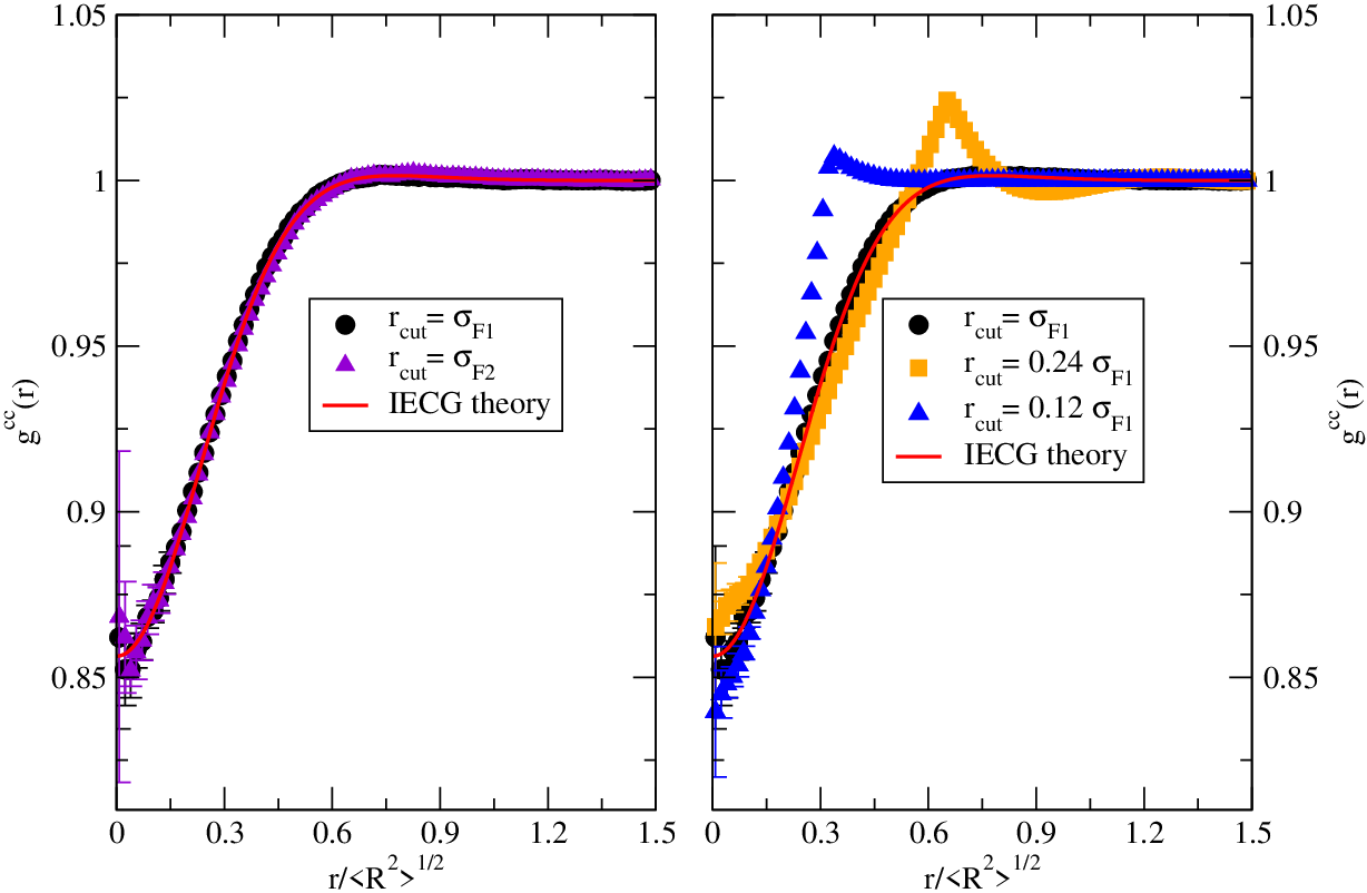
The left panel of Figure 5 shows consistent RDFs for the polymer melts with represented by soft spheres at K at a monomer density of Å-3 when the IECG effective potential is truncated at and , both of which are consistent with the IECG theory predictions. It is worth mentioning that the RDFs calculated for the given samples are consistent with the atomistic simulations.10 The right panel of Figure 5 shows that the inaccurate truncation of the IECG effective potential can result in significant errors in RDFs. The blue triangles show the RDF when the effective CG potential is truncated at a distance of about , which results in significant deviations in the correlation holes as compared to the accurate RDF. The deviations in the correlation hole is less pronounced when the effective CG potential is truncated at a distance of about (orange squares), but artificial peak and minimum appear in the RDF. Making use of a distance of about to truncate the potential still introduces an artificial peak but less pronounced than the red squares (results not shown).
Note that for the homogeneous systems studied in this work, the long-ranged CG corrections10 can be used to accurately compute the properties of interest such as pressure. In fact, the tail CG corrections turn out to work reasonably well for the estimation of the pressure obtained from various truncation of the effective CG potential when the MD simulations are stable. For instance, the values of pressure corrected with the CG long-range contributions for the relevant data presented in Figure 5 are about atm, which are in agreement with the atomistic simulation results (See Figure 2). This advancement in treating the long-range CG interactions in the IECG simulations reasonably results in the consistencies of various levels of CG with the atomistic simulation results in properties such as RDF and pressure.
In addition, Table 2 shows that larger values of are used for the IECG simulations of high-resolution multi-site CG models than for the soft sphere model, for a polymer melt with . This is because as the level of CG decreases and the range of the effective CG potential decreases, the curvature of the repulsive part of the effective CG potential becomes sharper such that relatively larger values of are required to avoid the failure of the MD algorithm. As discussed in Section 4.2.4, for a polymer melt represented by a given CG resolution, the curvature of the effective CG potential alters significantly less with varying density and temperature. This suggests that the optimum values do not change considerably for a polymer melt at a given degree of polymerization, in the range of temperature and density studied here.
Note that the system sizes in the standard IECG simulations is determined from the appropriate and . If one is not interested in problems that require large-scale simulations as discussed above, the boxlength in the IECG simulation can be set to be somewhat greater than twice as much as , which suggests that the number of pairwise interactions would be highest for the soft sphere models. In Table 2 the values of the box length are reported as . As the CG resolution increases, the range of potential decreases and at a given CG resolution one may use the system sizes close to the system sizes in the atomistic simulations such as the ten CG site model of polymer melt with as shown in Table 2 and Figure 4.
It is worth noting that a relatively small value of is required when the effective CG potential is truncated at larger distances, such as at the second zero of the force . This is mainly due to the large volume accessible to store the Verlet neighbor list when the effective CG potential is truncated at large distances and also the change in the curvature of the effective CG potential close to .
4.2.4 Density and Temperature Dependence: Range of the Effective CG Potential
Noting that the effective IECG potential is in fact a free energy, as the density and temperature increases for a given polymer melt, the first zero of the force, , increases in the IECG approach (see our previous work for the details10). Figure 6 illustrates this for a polymer melt with , when it is represented by soft sphere and six CG site models. This has implications on the computational efficiency of the IECG simulations. Making use of eq 8 and estimating the standard volume of the simulation box as and the and values and , respectively, the number of nonbonded pairwise interactions can be calculated as follows:
| (10) |
where , and is the site density.

Therefore, at a given temperature as the site density and consequently increases, the number of pairwise interactions in an IECG simulation can increase. This increase is more pronounced for the soft sphere models than the six CG site models. Similarly, at a given density, as the temperature increases so does ; therefore, the number of pairwise interactions in an IECG simulation can increase. It is worth noting that the curvature of the IECG effective potential slightly changes at various temperatures and densities, which allows one to use the close values to the optimum neighbor skin distances reported in Table 2.
4.3 Timestep ()
The equation of motions in MD simulations are integrated using finite difference algorithms, such as the Verlet integration algorithm3, which can lead to errors if the suitable timestep is not chosen, because making use of very large timesteps can cause numerical instabilities. Meanwhile, the larger the timestep, the more rapid sampling of the phase space, and the longer the timescale reached by the simulation. The MD timestep may be selected to be one or two orders of magnitude smaller than the characteristic timescale,, of the fastest motion of the system. In atomistic simulations, it is typical to adopt a timestep of femtoseconds, as will be discussed below. Similarly, the timestep in a given CG-MD simulation should be smaller than the fastest motion in the CG system.
Different CG models afford different timesteps, depending on the level of resolution of the CG model. We compare the IECG models in soft sphere and multi-site representations to other models of polymers, including the united atom models,60; 21 the MARTINI CG models,61 and the CG model by Grest and coworkers.5 Starting from all atom MD simulations of simple polymeric systems, where the shortest lengthscale is the atomistic lengthscale of nm, the fastest motions of the system involve C-H vibrations, which restricts one to use timesteps of fs.62; 63 In the united atom models, the fast vibrations of the C-H bonds are averaged out, and the CH, CH2 and CH3 atomic groups are treated as single rigid particles, allowing one to have access to about nm lengthscale resolutions and to use a timestep of fs in standard MD simulations.21 It is worth mentioning that multiple timestep methods such as Reversible REference System Propagator Algorithm (RESPA)64 can yield times speed-up in MD of all atom or united atom simulations, but they are less efficient in parallel MD simulations due to CPU communication. Neglecting the hydrogen atoms and on average representing four heavy atoms by a single interaction site, the MARTINI force field,65; 61; 66; 67; 68 developed to study biomolecular systems, allows for timesteps of fs in MD simulations, when an appropriate update of the Verlet neighbor lists is adopted. Recently, Grest et al. developed a CG model, which groups from two to up to six CH2 units into one CG unit, giving access to timesteps ranging from to fs in their MD simulations.5 Compared to the IECG models, the aforementioned CG models are low-level CG models.
In the IECG simulations, the appropriate timesteps may be estimated from the characteristic timescales as . For the soft sphere models, the characteristic timescale is given as
| (11) |
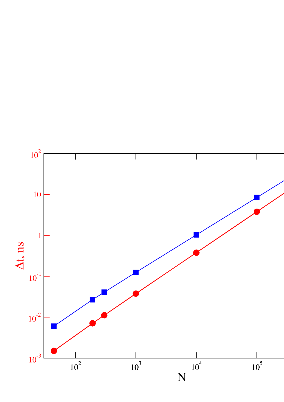
where is the mass of soft sphere and is the mean-square end-to-end polymer distance. This time is related to the mean time between soft sphere collisions. Depending on the degree of polymerization () and the level of molecular CG, this characteristic timescale for soft sphere models may range from picosecond for to microsecond for ; therefore, as shown in Figure 7, appropriate theoretical timesteps may range from hundreds of femtoseconds to tens of nanoseconds in the IECG simulations. This is another advantage of the IECG method in comparison with the high-resolution CG methods discussed above, where the timestep usually does not exceed tens of femtosecond.
In the practical application of MD simulations, one has to carefully consider the Verlet neighbor list updates to set up the appropriate timesteps, which should obey the following relationship:
| (12) |
where is the number of timesteps between two consecutive updates, is the velocity of a given CG site, which directly depends on the temperature.
Considering the frequency of updating the Verlet neighbor lists, CG timesteps larger than the characteristic timescale will result in the traveling of soft particles through distances larger than the (sub)domain, in a time prior to the (sub)domain calculation, which distorts the trajectory in phase space of the system, and affects the properties calculated from time averages. In other words, when the Verlet lists and the subdomains are built, for instance in the combined Verlet list and link-cell algorithms, particles may be lost if a large timestep is used and a particle travels a long distance before the list is updated. Therefore, the suitable timestep also depends on the sizes of the subdomain, which is related to the and values (see eq 12).
In addition, truncating the potential at short leads to a more repulsive potential, so that in the given timestep the high repulsive forces can make the particles travel unphysically long distances, with consequent failure of the MD algorithm. Therefore, in similar conditions, as the value increases and the contribution of the attractive part of the potential is properly taken into account in the IECG method, a larger CG timestep can be used with less likelihood of the failure of the MD algorithms.
Our MD simulations suggest that an value of allows one to use the appropriate CG timesteps () using the standard update of the Verlet neighbor list in the IECG simulations. To assess the accuracy of the suitable timestep, a series of IECG-MD simulations were performed starting from the same equilibrated liquid configurations using the Nos-Hoover thermostat.
Pressure, RDFs, and mean-square displacements were tested. Figure 8 shows consistencies in the RDFs and mean square displacements when relatively small and large timesteps have been used in the IECG simulations of polymer melts with degrees of polymerization of at K and the monomer density of Å-3 with the polymer represented as one soft sphere. In addition, the IECG simulations result in the pressure value of atm, kinetic energy per particle of kcal mol-1, potential energy per particle of kcal mol-1, and temperature of K when timesteps less than ps and reasonable values of are used. Therefore, the IECG simulations show that making use of larger timesteps up to ps is possible for a polymer melt with when represented by soft spheres, with the caveat that one has to use reasonable values of and Nos-Hoover thermostat parameters. Note that other common thermostats such as Berendsen thermostat may also be used in the IECG simulations. It is worth mentioning that in cases where common thermostats are not efficient, a simple velocity rescaling method can allow one to get reasonable results (not shown here) while saving computational time due to the simplicity of the algorithm. This is because all ensembles in the thermodynamic limit should give consistent results.

In the multi-site CG model, the characteristic timescale corresponds to the highest frequency motion of the CG bond vibrations, where the effective bond potential in the IECG method for a given polymer melt, , is then given by
| (13) |
with the number of CG sites in which the polymer chain is partitioned, the bond length between CG sites, and the correction term that enforces the correct distributions between adjacent CG sites.
Approximating the force constant of the multi-site bond vibrations by the first term in eq 13, i.e., treating the effective potential as a harmonic oscillator, gives a relaxation time for the fastest modes of vibration, , which theoretically scales as
| (14) |
Note that in the IECG simulations, the bonded sites are given a bond potential derived from the direct Boltzmann inversion of the probability distribution of the effective bond length, where the details are discussed in our previous works.9; 12 Therefore, treating the effective potential as the harmonic oscillator, the relaxation times of the fastest modes of vibration, , theoretically scales as . However, in practice the choice of appropriate timestep also involves the range of the effective CG potential, the cutoff distances, the neighbor skin distances, and the frequency of updating the Verlet list. Therefore, it is useful to evaluate if the theoretical scaling is recovered directly from MD simulations.

The effect of CG resolutions on the timestep was empirically investigated for multi-site models in the IECG simulations using the update frequency mentioned in Section 3.2. Making use of the combined Verlet neighbor list and link-cell algorithms38, the maximum CG timesteps that don’t lead to numerical instability are observed in MD simulations for various levels of CG, while using one processor. Figure 9 shows the effect of the CG resolutions on this empirical CG timestep for the multi-site models of polymer melts with at a given state point. Making use of the standard cutoff distances and neighbor skin distances presented in Table 2, the empirical timestep is found to obey the theoretical scaling with the number of CG sites (eq. 14).
4.4 Dynamical Scaling Factor ()
In principle, the CG procedure results in relatively much smoother free energy surfaces than the atomistic description because local degrees of freedom are averaged out during coarse-graining. In addition, coarse-graining on various levels results in various shapes of CG units with different hydrodynamic radii and friction coefficients.33; 34; 36 Both contributions speed up the dynamics, which significantly enhance sampling of the phase space for a given system.
Starting from the first-principle Liouville equation and applying the Mori-Zwanzig projection operator technique,69 we derived Generalized Langevin Equations (GLE) for the atomistic and for the IECG representation.33; 34; 36 The two GLEs differ in the linear term, which contains the entropic contribution due to the smoothing of the free energy landscape following CG, and in the memory function, which leads to different site friction coefficients. Both corrections are essential to reconstruct the atomistic dynamics from the IECG-MD simulation.
When accurate GLE formalisms are not formulated for the atomistic and CG representations, it is common practice to calculate empirically a numerical scaling factor by directly comparing dynamical quantities such as the mean square displacement (MSD), or diffusion coefficients, in the CG and atomistic simulations.32; 35; 5 Note that this empirical procedure doesn’t properly account for the physical motivation of the different dynamics that appear at varying levels of CG. However, given that we are interested only in determining the numerical gain following coarse-graining, we adopt this simple procedure to calculate the speed-up factors.
This requires running relatively long atomistic trajectories of polymer melts to reach the diffusive regime. Figure 10 demonstrates this for polymer melts with degrees of polymerizations of and in the relatively long atomistic simulations and the IECG simulations at various levels of CG. The diffusion coefficient, , in a system of identical particles can be computed from the linear part of the center of mass MSD as a function of time, , using the Einstein relation:47
| (15) |
where is the position of the center of mass of a given polymer. The dynamical scaling factor can then be estimated as the ratio between the diffusion coefficients from the CG and atomistic (AT) simulations, i.e. . We use this approach to compute the dynamical scaling factor for relatively short chain polymer melts. The results are presented in Table 3, where the diffusion constants in atomistic simulations were calculated as , , and Å2/ns for the polymer melts with degrees of polymerizations of , , and , respectively.

4.5 Overall Computational Efficiency
Overall, the computational efficiency of the IECG simulations, , can be reported as defined in eq 6, and reported in Table 3. The dynamical scaling factor turns out to dominate the other terms in eq 6 while considerable computational efficiency can be gained via the enhancement of the timestep in the IECG simulation. The computational gain based on the number of pairwise interactions, , can have positive and negative effects based on the level of CG or the CG resolution noting that the contribution of this term among other terms is lowest in eq 6. The range of potential significantly increases for soft sphere models such that the computational gain based on is inverse for the polymer melts with and when represented by soft spheres, but the computational gain of is achieved for the soft sphere model of polymer melt with .
For soft sphere models, as the level of CG increases, the dynamical scaling factor and the CG timesteps increase while the computational gain via in most cases decreases due to the long-range CG potential. For a given polymer melt, as the CG resolution increases the CG timesteps decrease, but the computational gain via requires care because it depends on the change in the values as well as in the values. In general, as the CG resolution increases, the values decrease, but the values, which are directly related to the optimum values of the CG timestep, can increase and compensate the computational gain obtained from the decrease in the values.
Although for the polymer melt with decreases as the CG resolution decreases, has a more complex behavior for the polymer melt with such that the values for four and six CG site models are almost equal due to the significant change in the value for the six CG site model. At the highest level of granularity, the CG model needs to recover the atomistic behavior. In a nutshell, Table 3 shows that the overall computational efficiency is highest for the soft sphere models and lowest for the highest resolution multi-site models.

Figure 11 summarizes the overall computational efficiency results. The left panel of Figure 11 shows millions magnitude computational efficiency for the soft spheres as the degree of polymerization increases while the right panel shows that the overall efficiency for a polymer melt with at various CG resolutions, which decreases as the level of CG decreases.
4.5.1 Parallel Scalability
Due to the importance of parallel computing, we complete our study with a discussion on the parallel scalability of the IECG simulations as compared with the atomistic simulations. A thorough description of fast parallel algorithms such as atom decomposition, force decomposition, spatial decomposition for MD simulations are given in ref (38). All three aforementioned methods balance computation optimally as , where is the number of interaction sites and is the number of processors and Newton’s third law is implemented for interactions between particle pairs inside a processor’s box.
Standard spatial decomposition algorithms subdivide the physical simulation domain into small three-dimensional boxes for each processor and uses two data structures: one for storing the particles in its box, which contains a complete set of data such as position, velocity, and Verlet neighbor lists, and the other one for particles in nearby boxes, which only stores particle positions and the six data exchange algorithm described in ref (38), which is used for exchanging all particle positions in adjacent boxes.
Added to the computation, which scales as , the communication scales as for relatively large problems and the memory scales as . Unlike the link-cell algorithm, the box length (sub-domain) may now be smaller, equal, or larger than the value. This has important implications for the IECG simulations because the long-range nature of the IECG effective potential requires using large values. Therefore, the sub-domain of a processor can be smaller than the value and the particle information is required from more distant boxes, which requires sending positions of a sub-domain to many neighbors and extra communication to acquire the required particle positions and forces.
Note that each processor computes forces on particles in its sub-domain using the ghost information from nearby processors, and processors communicate and store ghost particle information for particles that border their sub-domain. On the other hand, as discussed in section 4.2, as the level of CG decreases, the range of the effective CG potential decreases, and the total number of interactions can decrease in the IECG simulations. Therefore, it is more likely to lead to the communication overhead, which can lower/stop the speed-up for a given number of CPUs.
In the case of multi-site models, particles can move to new processors and molecular connectivity information must be exchanged and updated between processors. The extra coding to manipulate the appropriate data structures and optimize the communication performance of the data exchange subtracts from the parallel efficiency of the algorithm (see Figures 12 and 13 and the discussion below).

To use the computational resources effectively and reduce the time to solve a problem, efficient strong scaling is required. Figure 12 compares the strong scaling performance for the IECG simulations of polymer melts with represented by soft sphere and six CG site models with the atomistic simulation performance, which does not have considerable finite size effects for the structural and thermodynamical properties of interest. All simulations were performed on the compute nodes of the Comet supercomputer, a high-performance computing cluster provided by Extreme Science and Engineering Discovery Environment (XSEDE) resources,70 where the compute nodes consisted of Intel Xeon E5-2680v3 processors.
To minimize the communication in the spatial decomposition algorithm, the number of processors in each dimension was chosen to make each processor’s box cubic. The Verlet neighbor list was updated for each MD step for these sets of IECG simulations, which allowed us to use the spatial decomposition algorithm by adopting the appropriate CG timestep. The top panel presents the CPU strong scaling factor, when the performance is only reported in terms of MD step per second. Note that the dashed lines show parallel scalability (ideal scaling); therefore, excellent strong scaling is observed for the soft sphere and the atomistic models, while good strong scalability is shown for the six CG site model.
Due to the significant increase in the range of the effective CG potential, the soft sphere model in comparison with the six CG site and the atomistic models requires more computation time to complete one MD step. However, considering that a significantly larger CG timestep can be used for the soft sphere model as compared with the six site and atomistic models, the performance of soft sphere models considerably increases when the performance is reported in terms of ns per day. Note that due to the long-range effective CG potential for the soft sphere model, the simulation boxlength is the highest. In addition, larger CG timesteps can be used for serial runs as compared with the parallel runs due to the spatial decomposition algorithm and the enhanced dynamics of the CG system. For instance, it is possible that a bond between the CG sites becomes large: when a bond that straddles two subdomains becomes too large, one of the two CG sites forming the bond is no longer within the surrounding ghost CG units and the spatial decomposition algorithm practically fails. Indeed, it was found that as the size of subdomain is increased, the spatial decomposition algorithm can handle larger CG timesteps.

Figure 13 provides a detailed analysis of the parallel scalability for the aforementioned IECG and atomistic simulations. In summary, it shows that the overall time consumption for a relatively short number of processors is due to the nonbonded force evaluations, but it switches to the communication for a relatively large number of processors. Considering the Message Passing Interface timing breakdown38, the right top panel shows the percentage of communication time as the number of processors increases. As the number of processors increase, the percentage of communication increases with the highest slope for the six site model most likely due to the effective CG potential that is more long-ranged than the atomistic one and the absence of molecular connectivity information in the soft sphere model. The range of potential in the atomistic simulations is much less than the IECG simulations, which results in lower percentage of communication for exchanging the particles from nearby boxes in the atomistic simulations.
The left bottom panel of Figure 13 shows that there is a crossover in the percentage of nonbonded force calculations in MD simulations for the aforementioned models. The percentage of nonbonded force calculations is almost a plateau for a relatively small number of processors, but the crossover occurs at a relatively large number of processors, which is highest for the soft sphere model. In addition, unlike the percentage of communication time, which almost reaches a plateau for a large number of processors, the percentage of nonbonded force computation time for all models does not show plateau behavior for a relatively large number of processors.
The right bottom panel of Figure 13 shows the percentage of Verlet neighbor list calculation time, which is usually highest for the soft sphere model. This is expected as the range of the effective CG potential and the number of pairwise interactions are the highest for the soft sphere model. Similarly the six CG site model requires more percentage of consumption time for all processors as compared to the atomistic one, noting that the consumption time for the atomistic neighbor list calculations is almost constant for a relatively large number of processors.
To end this section, it is worth mentioning that one can adjust the size and shape of processor sub-domains within the simulation box to balance the number of particles (load balance) more evenly across processors. The load balancing used in the above analysis was static in the sense that one performs the balancing once, before MD simulations. In addition, the analysis was done for relatively homogeneous systems, where uniform load balancing naturally emerges. For the inhomogeneous systems, other approaches such as the Hilbert space-filling curve and cell task methods as discussed in the literature 71; 72; 59 may be used.
5 Conclusions
The IECG approach is a high level CG method, which allows modeling systems consisting of long chain polymers. It can be developed from a top-down or bottom-up approach. The bottom-up approach allows one to directly compare the computational efficiency of the IECG simulations with the atomistic simulations. Due to the nature of long-range effective IECG potential, relatively larger system sizes than the atomistic simulations are required when computing relevant structural and thermodynamical properties. On the basis of the data just discussed, it is clear that the selection of suitable parameters plays a pivotal role in controlling the computational efficiency of the IECG simulations.
The recommendations from this work are to employ the following parameters for the relevant IECG simulations at various state points: (i) truncating the effective CG potential at distances, which include the attractive part of the effective CG potential/force allows accurate and efficient IECG simulations; a cutoff distance of turns out to fulfill this requirement, where is the first zero of the force over the range of distance greater than zero; (ii) considering the neighbor skin distance and the frequency of updating the Verlet neighbor list, a timestep of of the shortest characteristic time, , may be used for the IECG simulations, where can be estimated from eq 11 and eq 14; (iii) the optimum neighbor skin distance depends on curvature of the effective CG potential, the CG timestep, and the frequency of updating the Verlet neighbor list; as the level of CG changes for a given polymer melt, the curvature of the effective CG potential changes, which can affect the suitable neighbor skin distance; for a high level of CG the neighbor skin distances of work reasonably well with the standard frequency of the Verlet neighbor list update, but as the effective CG potential decays steeper for high resolution multi-site models relatively larger neighbor skin distances such as are recommended; note that the curvature of the effective CG potential, at relevant densities and temperatures and at the level of CG reported here, does not change considerably; (iv) while the spatial decomposition algorithm can be used to speed up MD simulations using a large number of processors, the sub-domain size decreases, which can influence the selection of the suitable parameters; for instance, depending on the number of processors, smaller CG timesteps may be used for parallel MD simulations; (v) when the physical problem involves large correlation lengths associated with the properties of interest for long chain polymer melts, atomistic simulations, which use relatively small system sizes, are more likely to be unsuccessful and it is inevitable to use relatively large system sizes to avoid finite size effects; in these circumstances, a soft sphere model is perhaps the most efficient model to study the global properties, considering that the free energy surface is smoothest.
The soft sphere and multi-site models in the IECG simulations allow one to treat the same molecular system at different resolutions while offering millions of magnitude computational efficiency (as determined by eq 6 and presented in Table 3 for various polymer melts). Considering the suitable MD parameters in the IECG and atomistic MD simulations, the soft sphere models turn out to be computationally most efficient while the high-resolution multi-site models give more detailed descriptions of the structure on the local scale. The conclusions reached with regard to the optimal choice of the CG-MD parameters and the computational efficiency should also be applicable to other high level CG approaches.
References
- [2] Rahman, A.; Stillinger, F. H. Molecular Dynamics Study of Liquid Water. J. Chem. Phys. 1971, 55, 3336–3359.
- [3] Allen, M. P.; Tildesley, D. J. Computer Simulations of Liquids; Oxford University Press: Oxford, 1987.
- [4] Frenkel, D.; Smit, B. Understanding Molecular Simulations, 2nd ed.; Academic Press: San Diego, 2002.
- [5] Salerno, K. M.; Agrawal, A.; Perahia, D.; Grest, G. S. Resolving Dynamic Properties of Polymers through Coarse-Grained Computational Studies. Phys. Rev. Lett. 2016, 116, 3–7.
- [6] Reith, D.; Pütz, M.; Müller-Plathe, F. Deriving Effective Mesoscale Potentials from Atomistic Simulations. J. Comp. Chem. 2003, 24, 1624–1636.
- [7] Harmandaris, V. A.; Adhikari, N. P.; Van Der Vegt, N. F. A.; Kremer, K. Hierarchical Modeling of Polystyrene: From Atomistic to Coarse-Grained Simulations. Macromolecules 2006, 39, 6708–6719.
- [8] Guenza, M. G. Coarse-Grained Modeling of Biomolecules; Taylor & Francis Group, LLC; CRC Press: Boca Raton, 2018; Chapter 2, p 27.
- [9] Clark, A. J.; McCarty, J.; Guenza, M. G. Effective Potentials for Representing Polymers in Melts as Chains of Interacting Soft Particles. J. Chem. Phys. 2013, 139, 124906.
- [10] Dinpajooh, M.; Guenza, M. G. On the Density Dependence of the Integral Equation Coarse-Graining Effective Potential. J. Phys. Chem. B 2018, 122, 3426–3440.
- [11] Clark, A. J.; Mccarty, J.; Lyubimov, I. Y.; Guenza, M. G. Thermodynamic Consistency in Variable-Level Coarse Graining of Polymeric Liquids. Phys. Rev. Lett. 2012, 109, 168301.
- [12] McCarty, J.; Clark, A. J.; Copperman, J.; Guenza, M. G. An Analytical Coarse-Graining Method which Preserves the Free Energy, Structural Correlations, and Thermodynamic State of Polymer Melts from the Atomistic to the Mesoscale. J. Chem. Phys. 2014, 140, 204913.
- [13] Dinpajooh, M.; Guenza, M. G. Thermodynamic Consistency in the Structure-based Integral Equation Coarse-Grained Method. Polymer 2017, 117, 282–286.
- [14] Yatsenko, G.; Sambriski, E. J.; Nemirovskaya, M. A.; Guenza, M. Analytical Soft-Core Potentials for Macromolecular Fluids and Mixtures. Phys. Rev. Lett. 2004, 93, 257803.
- [15] Clark, A. J.; Guenza, M. G. Mapping of Polymer Melts onto Liquids of Soft-Colloidal Chains. J. Chem. Phys. 2010, 132, 044902.
- [16] McCarty, J.; Clark, A. J.; Lyubimov, I. Y.; Guenza, M. G. Thermodynamic Consistency between Analytic Integral Equation Theory and Coarse-Grained Molecular Dynamics Simulations of Homopolymer Melts. Macromolecules 2012, 45, 8482–8493.
- [17] Carnahan, N. F.; Starling, K. E. Thermodynamic Properties of a Rigid-Sphere Fluid. J. Chem. Phys. 1970, 53, 600–603.
- [18] Carbone, P.; Varzaneh, H. A. K.; Chen, X.; Müller-Plathe, F. Transferability of Coarse-Grained Force Fields: The Polymer Case. J. Chem. Phys. 2008, 128, 064904.
- [19] Harmandaris, V. A.; Mavrantzas, V. G.; Theodorou, D. N.; Kröger, M.; Ramírez, J.; Ottinger, H. C.; Vlassopoulos, D. Crossover from the Rouse to the Entangled Polymer Melt Regime: Signals from Long, Detailed Atomistic Molecular Dynamics Simulations, Supported by Rheological Experiments. Macromolecules 2003, 36, 1376–1387.
- [20] Das, A.; Lu, L.; Andersen, H. C.; Voth, G. A. The Multiscale Coarse-Graining Method. X. Improved Algorithms for Constructing Coarse-grained Potentials for Molecular Systems. J. Chem. Phys. 2012, 136, 194114.
- [21] Ramos, J.; Vega, J. F.; Martinez-Salazar, J. Molecular Dynamics Simulations for the Description of Experimental Molecular Conformation, Melt Dynamics, and Phase Transitions in Polyethylene. Macromolecules 2015, 48, 5016–5027.
- [22] Cao, Z.; Voth, G. A. The Multiscale Coarse-Graining Method. XI. Accurate Interactions Based on the Centers of Charge of Coarse-grained Sites. J. Chem. Phys. 2015, 143, 243116.
- [23] Izvekov, S.; Voth, G. A. Multiscale Coarse Graining of Liquid-State Systems. J. Chem. Phys. 2005, 123, 134105.
- [24] Shell, M. S. The Relative Entropy is Fundamental to Multiscale and Inverse Thermodynamic Problems. J. Chem. Phys. 2008, 129, 144108.
- [25] Brini, E.; Algaer, E. A.; Ganguly, P.; Li, C.; Rodríguez-Ropero, F.; van der Vegt, N. F. A. Systematic Coarse-Graining Methods for Soft Matter Simulations - a Review. Soft Matter 2013, 9, 2108–2119.
- [26] Dunn, N. J.; Noid, W. G. Bottom-up Coarse-Grained Models that Accurately Describe the Structure, Pressure, and Compressibility of Molecular Liquids. J. Chem. Phys. 2015, 143, 243148.
- [27] Rudzinski, J. F.; Noid, W. G. Bottom-up Coarse-Graining of Peptide Ensembles and Helix-coil Transitions. J. Chem. Theory Comput. 2015, 11, 1278–1291.
- [28] Avendaño, C.; Lafitte, T.; Galindo, A.; Adjiman, C. S.; Jackson, G.; Müller, E. A. SAFT- Force Field for the Simulation of Molecular Fluids. 1. A Single-site Coarse grained Model of Carbon Dioxide. J. Phys. Chem. B 2011, 115, 11154–11169.
- [29] Gil-Villegas, A.; Galindo, A.; Whitehead, P. J.; Mills, S. J.; Jackson, G.; Burgess, A. N. Statistical Associating Fluid Theory for Chain Molecules with Attractive Potentials of Variable Range. J. Chem. Phys. 1997, 106, 4168–4186.
- [30] Hsu, D. D.; Xia, W.; Arturo, S. G.; Keten, S. Thermomechanically Consistent and Temperature Transferable Coarse-Graining of Atactic Polystyrene. Macromolecules 2015, 48, 3057–3068.
- [31] Kremer, K.; Grest, G. S. Dynamics of Entangled Linear Polymer Melts: A Molecular-Dynamics Simulation. J. Chem. Phys. 1990, 92, 5057–5086.
- [32] Fritz, D.; Herbers, C. R.; Kremer, K.; van der Vegt, N. F. A. Hierarchical Modeling of Polymer Permeation. Soft Matter 2009, 5, 4556.
- [33] Lyubimov, I. Y.; McCarty, J.; Clark, A.; Guenza, M. G. Analytical Rescaling of Polymer Dynamics from Mesoscale Simulations. J. Chem. Phys. 2010, 132, 224903.
- [34] Lyubimov, I.; Guenza, M. G. First-principle Approach to Rescale the Dynamics of Simulated Coarse-Grained Macromolecular Liquids. Phys. Rev. E 2011, 84, 16–18.
- [35] Fritz, D.; Koschke, K.; Harmandaris, V. A.; van der Vegt, N. F. A.; Kremer, K. Multiscale Modeling of Soft Matter: Scaling of Dynamics. Phys. Chem. Chem. Phys. 2011, 13, 10412.
- [36] Lyubimov, I. Y.; Guenza, M. G. Theoretical Reconstruction of Realistic Dynamics of Highly Coarse-Grained cis-1,4-Polybutadiene Melts. J. Chem. Phys. 2013, 138, 12A546.
- [37] Davtyan, A.; Voth, G. A.; Andersen, H. C. Dynamic Force Matching: Construction of Dynamic Coarse-Grained Models with Realistic Short Time Dynamics and Accurate Long Time Dynamics. J. Chem. Phys. 2016, 145, 224107.
- [38] Plimpton, S. Fast Parallel Algorithms for Short-Range Molecular Dynamics. J. Comp. Phys. 1995, 117, 1–19.
- [39] Bussi, G.; Donadio, D.; Parrinello, M. Canonical Sampling Through Velocity Rescaling. J. Chem. Phys. 2007, 126, 014101.
- [40] Halverson, J. D.; Brandes, T.; Lenz, O.; Arnold, A.; Bevc, S.; Starchenko, V.; Kremer, K.; Stuehn, T.; Reith, D. ESPResSo++: A Modern Multiscale Simulation Package for Soft Matter Systems. Comput. Phys. Commun. 2013, 184, 1129–1149.
- [41] Verlet, L. Computer "Experiment" on Classical Fluids. I. Thermodynamical Properties of Lennard-Jones Molecules. Phys. Rev. 1967, 159, 98.
- [42] Chialvo, A. A.; Debenedetti, P. G. On the Use of the Verlet Neighbor List in Molecular Dynamics. Comput. Phys. Commun. 1990, 60, 215–224.
- [43] Schweizer, K. S.; Gurro, J. G. Integral Equation Theories of the Structure, Thermodynamics, and Phase Transitions of Polymer Fluids. Adv. Chem. Phys. 1997, 98, 1–142.
- [44] Stanley, H. E. Introduction to Phase Transitions and Critical Phenomena; Oxford University Press: New York, 1987.
- [45] Stukan, M. R.; Ivanov, V. A.; Muller, M.; Paul, W.; Binder, K. Finite Size Effects in Pressure Measurements for Monte Carlo Simulations of Lattice Polymer Models. J. Chem. Phys. 2002, 117, 9934–9941.
- [46] McCarty, J.; Lyubimov, I. Y.; Guenza, M. G. Effective Soft-Core Potentials and Mesoscopic Simulations of Binary Polymer Mixtures. Macromolecules 2010, 43, 3964–3979.
- [47] Hansen, J. P.; McDonald, I. R. Theory of Simple Liquids; Academic Press: Amsterdam, 2003.
- [48] Schweizer, K. S.; Curro, J. G. Integral-Equation Theory of the Structure of Polymer Melts. Phys. Rev. Lett. 1987, 58, 246–249.
- [49] Schweizer, K. S.; Curro, J. G. RISM Theory of Polymer Liquids: Analytical Results for Continuum Models of Melts and Alloys. Chem. Phys. 1990, 149, 105–127.
- [50] Chandler, D.; Andersen, H. C. Optimized Cluster Expansions for Classical Fluids. II. Theory of Molecular Liquids. J. Chem. Phys. 1972, 57, 1930–1937.
- [51] Guenza, M.; Schweizer, K. S. Fluctuations Effects in Diblock Copolymer Fluids: Comparison of Theories and Experiment. J. Chem. Phys. 1997, 106, 7391–7410.
- [52] Yatsenko, G.; Sambriski, E. J.; Guenza, M. G. Coarse-grained Description of Polymer Blends as Interacting Soft-Colloidal Particles. J. Chem. Phys. 2005, 122, 054907.
- [53] Sankar, U. K.; Tripathy, M. Dispersion, Depletion, and Bridging of Athermal and Attractive Nanorods in Polymer Melt. Macromolecules 2015, 48, 432–442.
- [54] Louis, A. A.; Bolhuis, P. G.; Hansen, J. P.; Meijer, E. J. Can Polymer Coils Be Modeled as "Soft Colloids"? Phys. Rev. Lett. 2000, 85, 2522–2525.
- [55] Dinpajooh, M.; Guenza, M. G. The Integral Equation Coarse-Graining Method. https://iecgsim.uoregon.edu.
- [56] McCarty, J.; Lyubimov, I. Y.; Guenza, M. G. Multiscale Modeling of Coarse-Grained Macromolecular Liquids. J. Phys. Chem. B 2009, 113, 11876–11886.
- [57] Martin, M. G.; Siepmann, J. I. Transferable Potentials for Phase Equilibria. 1. United-Atom Description of n -Alkanes. J. Phys. Chem. B 1998, 102, 2569–2577.
- [58] Mei, J.; Davenport, J. W.; Fernando, G. W. Analytic Embedded-atom Potentials for FCC Metals: Application to Liquid and Solid Copper. Phys. Rev. B. 1991, 43, 4653–4658.
- [59] Meyer, R. Efficient Parallelization of Molecular Dynamics Simulations with Short-Ranged Forces. J. Phys. Conf. Ser. 2014, 540, 012006.
- [60] Paul, W.; Yoon, D. Y.; Smith, G. D. An Optimized United Atom Model for Simulations of Polymethylene Melts. J. Chem. Phys. 1995, 103, 1702–1709.
- [61] Marrink, S. J.; Risselada, H. J.; Yefimov, S.; Tieleman, D. P.; De Vries, A. H. The MARTINI Force Field: Coarse-Grained Model for Biomolecular Simulations. J. Phys. Chem. B 2007, 111, 7812–7824.
- [62] Müller-Plathe, F. Coarse-graining in Polymer Simulation: From the Atomistic to the Mesoscopic Scale and Back. ChemPhysChem 2002, 3, 754–769.
- [63] Siu, S. W. I.; Pluhackova, K.; Böckmann, R. A. Optimization of the OPLS-AA Force Field for Long Hydrocarbons. J. Chem. Theory Comput. 2012, 8, 1459–1470.
- [64] Tuckerman, M.; Berne, B. J.; Martyna, G. J. Reversible Multiple Time Scale Molecular Dynamics. J. Chem. Phys. 1992, 97, 1990–2001.
- [65] Marrink, S. J.; de Vries, A. H.; Mark, A. E. Coarse Grained Model for Semiquantitative Lipid Simulations. J. Phys. Chem. B 2004, 108, 750–760.
- [66] Murtola, T.; Bunker, A.; Vattulainen, I.; Deserno, M.; Karttunen, M. On Using a Too Large Integration Time Step in Molecular Dynamics Simulations of Coarse-Grained Molecular Models. Phys. Chem. Chem. Phys. 2009, 11, 1869.
- [67] Marrink, S. J.; Periole, X.; Tieleman, D. P.; de Vries, A. H. Comment on "On Using a Too Large Integration Time Step in Molecular Dynamics Simulations of Coarse-Grained Molecular Models". Phys. Chem. Chem. Phys. 2010, 12, 2254.
- [68] van Gunsteren, W. F.; Winger, M. Reply to the ’Comment on "On Using a Too Large Integration Time Step in Molecular Dynamics Simulations of Coarse-grained Molecular Models"’. Phys. Chem. Chem. Phys. 2010, 12, 2254.
- [69] Zwanzig, R. Nonequilibrium Statistical Mechanics; Oxford University Press: New York, 2001.
- [70] Towns, J.; Cockerill, T.; Dahan, M.; Foster, I.; Gaither, K.; Grimshaw, A.; Hazlewood, V.; Lathrop, S.; Lifka, D.; Peterson, G. D.; Roskies, R.; Scott, J. R.; Wilkins-Diehr, N. XSEDE: Accelerating Scientific Discovery. Comput. Sci. Eng. 2014, 16, 62–74.
- [71] Grime, J. M. A.; Voth, G. A. Highly Scalable and Memory Efficient Ultra-Coarse-Grained Molecular Dynamics Simulations. J. Chem. Theory Comput. 2014, 10, 423–431.
- [72] Brázdová, V.; Bowler, D. R. Automatic Data Distribution and Load Balancing with Space-filling Curves: Implementation in CONQUEST. J. Phys. Condens. Matt. 2008, 20, 275223.