Lifetime of Majorana qubits in Rashba nanowires with non-uniform chemical potential

Introduction.— The main benefit of topological quantum computing [1, 2, 3, 4, 5] is the possibility to encode quantum information in degenerate many-body ground states (GSs) in such a way that it is free of decoherence in the ideal case. A realization of such topologically protected GSs are zero-energy Majorana bound states (MBSs) in a topological superconductor (TSC) [6, 7, 8, 9, 10, 11]. One of the most promising systems are semiconducting Rashba nanowires (NWs) in proximity with an $s$-wave superconductor and in the presence of magnetic fields [12, 13, 14, 15, 16, 17, 18, 19, 20, 6, 22, 23, 24, 25, 26, 27, 28, 29, 30, 31, 32, 33, 34, 35].

In realistic cases where the system is subject to random state fluctuations, the TSC may be driven out of its GS. This happens if the TSC is coupled to ungapped [36] or gapped [37, 38] fermionic baths as well as to fluctuating bosonic fields [37] (e.g. phonons [37, 39] or electromagnetic environments [39]). A similar mechanism is due to thermal fluctuations of a gate potential [40, 41]. In this case the TSC stays in the GS only for a finite lifetime $\tau$ after which the quantum state of the qubit associated with MBSs will leak out of the computational space, resulting in losing the quantum information. The corresponding rate of excitations caused by thermal fluctuations is exponentially small at low temperatures [42]. Estimations in Ref. 40 show that in order to maintain $\tau$ as high as microseconds the temperature should not exceed $\Delta/5$, where $\Delta$ is the gap in the TSC (we set $k_{B}=1$). This estimation is justified for the simple case of uniform system parameters. However, in many schemes of topological quantum computing the localized MBSs must be braided around each other, which requires to change the parameters locally. For example, in Ref. 43, the gates control local chemical potentials so that the NW is separated into topological and trivial sections with MBSs at the interfaces, which allows one to manipulate the non-local fermions which form the Majorana qubit. Recent studies [44, 45, 46, 47, 48, 49, 50, 51] were focused on the case where detection of MBSs and reading out associated qubits can be achieved by tuning gates to couple MBSs to quantum dots [52, 53, 54, 55, 56, 57, 58, 51, 59]. Since gates are located near the topological NWs they create a non-uniform electrostatic potential and can tune the ends of the NWs out of the topological phase.

It has been shown in Ref. 60 that non-localities introduced by braiding restricts the lifetime of qubits due to errors occurring during their motion. In this paper we will show that at finite temperatures the non-uniformity of system parameters can strongly reduce the lifetime even for immobile MBSs. As a model we consider a 1D proximitized Rashba NW with a non-uniform chemical potential induced by gates (see Fig. 1). We also study how $\tau$ changes if a part of the NW is tuned out of the topological phase. We develop a microscopic formalism with Keldysh techniques to treat the noisy gates and to calculate $\tau$. This approach can be easily generalized to other bosonic modes such as plasmons, phonons etc. Using realistic parameters, we are able to predict the optimal regime of operation for Majorana qubits.

Model.— We consider a setup consisting of a spinful single-band NW with a proximity-induced superconducting gap $\Delta_{sc}$. The Rashba spin-orbit interaction (SOI) of strength $\alpha_{R}$ sets the spin quantization axis to be perpendicular to the NW and corresponds to the SOI energy $E_{so}=m_{0}\alpha_{R}^{2}/(2\hbar^{2})$, where $m_{0}$ is the effective electron mass. A magnetic field (corresponding to the Zeeman energy $\Delta_{Z}$) is applied along the NW. The tight-binding Hamiltonian describing the NW has the form [61]

where $t=\hbar^{2}/(2m_{0}a^{2})$ is the hopping amplitude, $c_{s,j}$ annihilates an electron with spin $s$ at site $j$ with coordinate $x_{j}$, $\mu(x)$ is a non-uniform chemical potential (measured from $E_{so}$), and $\sigma^{x,y}$ are the Pauli matrices.

In the following we assume that the Zeeman energy is always larger than the superconducting gap, $\Delta_{Z}>\Delta_{sc}$. The chemical potential $\mu(x)$ is controlled by local gates and the NW is divided into a left and right section with lengths $L_{-}$ and $L_{+}$, respectively (see Fig. 1). We model the non-uniformity of $\mu(x)$ by a function with linear slope within the interface between the sections, $|x|<l_{0}$, where $l_{0}$ is the transition length,

Here, $\Theta(x)$ is the Heaviside step-function and $\mu_{+}$ is the value of chemical potential in the right section. In the left section, the chemical potential is set to the SOI energy, $\mu=0$, such that the left section is always in the topological phase. The gap in the left section is $\Delta_{-}\approx 2\Delta_{sc}\sqrt{E_{so}/\Delta_{Z}}$ for weak SOI, $E_{so}\ll\Delta_{Z}$, while $\Delta_{-}\approx\min\{\Delta_{sc},|\Delta_{Z}-\Delta_{sc}|\}$ for strong SOI, $E_{so}\gg\Delta_{Z}$. The gap in the right section is given by $\Delta_{+}=|\Delta_{Z}-\sqrt{\Delta_{sc}^{2}+\mu_{+}^{2}}|$ near the topological phase transition, $\mu_{+}\approx\mu^{*}=\sqrt{\Delta_{Z}^{2}-\Delta_{sc}^{2}}$. The corresponding decay lengths are defined as $\xi_{\pm}=\hbar v_{F\pm}/\Delta_{\pm}$, where $v_{F\pm}$ are the Fermi velocities, depending on $\Delta_{Z}$ and $\mu_{+}$.

Andreev bound states.— For $\mu_{+}>\mu^{*}$ [62], the right section is trivial, and one of the MBSs is located at the interface between the sections. There also emerge a number of fermionic states with energies below the gaps $\Delta_{\pm}$ (see Fig. 2): (i) Right Andreev bound states (RABSs) localized at the right end of the NW; (ii) Interface Andreev bound states (IABSs) localized at the interface between the sections [22, 63, 64, 65, 66, 67, 28, 68, 69, 70, 71, 72]. The IABSs emerge when $l_{0}$ exceeds the minimum of the two decay lengths, $l_{0}\gtrsim\min\{\xi_{+},\xi_{-}\}$. The energies of IABSs can be significantly less than the gaps $\Delta_{\pm}$, if $\mu_{+}$ is close to the critical value, $\mu_{+}\gtrsim\mu^{*}$, or if $l_{0}$ is much longer than $\xi_{-}$ (see Fig. 2). In the latter case the energy of IABSs decreases with increasing $l_{0}$ as $\varepsilon\sim\sqrt{\alpha_{R}\mu^{*}\mu_{+}/(2\Delta_{Z}l_{0})}\propto l_{0}^{-1/2}$ [73] If there is a mechanism which allows to change the system from the GSs to some excited states, these IABSs will play a crucial role in determining the lifetime of the GS.

Lifetime of GS in topological NW.— In physical setups the local electrostatic potentials are tuned by gates. The charges in the gates can fluctuate giving rise to fluctuations of the gate potentials. For simplicity, we consider a single normal metal gate located at distance $d_{0}$ from the NW. We denote the position of electrons in the gate by $\mathbf{R}=(R_{x},\mathbf{R}_{\bot})$, where $R_{x}$ is the coordinate along the NW, and $\mathbf{R}_{\bot}$ denotes the remaining coordinates. The gates are modeled by non-interacting electrons in $D$ dimensions (we consider $D=2,3$) and described by the gate Hamiltonian,

where $\Psi_{s}$ is a field operator for electrons with spin $s$, $\varepsilon_{F}^{(g)}$ the corresponding Fermi energy, and $m_{g}$ the effective electron mass. The electrostatic potential $\varphi(x_{i})$ induced by the gate electrons at site $i$ of the NW is given by

where $e$ is electron charge and $U(\mathbf{R},x_{i})$ the potential at site $i$ of the NW created by a unit point charge located at position $\mathbf{R}$ in the gate. For screened electron-electron interactions it is given by the Yukawa potential [74],

Here, $\epsilon$ is the dielectric constant of the NW, $\epsilon_{0}$ is the vacuum permittivity, $d(\mathbf{R},x_{i})$ the distance between the point $\mathbf{R}$ in the gate and the $i$-th site in the NW, and $\lambda\sim d_{0}$ the screening length. The main contribution to the potential created by the gate stems from electrons located in a layer of width $\lambda$ near the gate surface, and we replace $U$ with a simplified delta-function potential, $U=U_{0}\lambda^{D}\delta(x_{i}-R_{x})\delta(\mathbf{R}_{\bot})$, with amplitude $U_{0}\approx e^{-d_{0}/\lambda}/(4\pi\epsilon\epsilon_{0}d_{0})$. We note that the formalism developed below remains valid for general $U$. Finally, the coupling of electrons in the NW to the fluctuating electrostatic potential $\varphi$ is described by the Hamiltonian

We focus on the gate fluctuations, $\delta\varphi=\varphi-\langle\varphi\rangle$, absorbing the mean value $\langle\varphi\rangle$ in $\mu$.

We calculate the lifetime of the GS using Keldysh techniques [75, 76]. The retarded Green function $\mathcal{D}^{R}$ for the bosonic fields $\delta\varphi$ corresponding to the Feynman diagram shown in Fig. 3a is given by

where, in energy representation, $\mathcal{G}^{R(A)}_{g}(\varepsilon)$ is the retarded (advanced) Green function for the gate electrons, $\mathcal{G}^{K}_{g}(\varepsilon)$ the Keldysh counterpart, and $\varepsilon$ is measured from the Fermi level $\varepsilon_{F}^{(g)}$.

For a 2D or 3D gate, the correlations are short-ranged and we find $\mathcal{G}^{R}_{g}(\mathbf{R},\mathbf{R}^{\prime},0)\approx-i\pi\nu_{D}k_{F}^{-D}\delta(\mathbf{R}-\mathbf{R}^{\prime})$ [76], where $\nu_{D}$ is the $D$-dimensional density of states at the Fermi level and $k_{F}$ the Fermi wavevector in the gate. For $\mathcal{G}_{g}^{K}$ we use the fluctuation-dissipation theorem (FDT), $\mathcal{G}_{g}^{K}(\varepsilon)=2i\tanh(\varepsilon/2T)\mathrm{Im}\mathcal{G}^{R}(\varepsilon)$. Performing the integrations in Eq. (7) we then get

where $g=\pi(\nu_{D}eU_{0})^{2}\lambda^{D}/k_{F}^{D}$ is the effective coupling constant. The Keldysh version again follows from the FDT, $\mathcal{D}^{K}(\omega)=2i\coth(\omega/2T)\mathrm{Im}\mathcal{D}^{R}(\omega)$.

Importantly, the fluctuations $\delta\varphi$ can excite the non-local fermion (shared by two MBSs) out of the GS. The Feynman diagram for the Keldysh self-energy $\Sigma$ corresponding to this process is shown in Fig. 3b. The real part of the retarded self-energy integrated over coordinates, $\Sigma^{R}(\varepsilon)=\int dxdx^{\prime}\;\Sigma^{R}(x,x^{\prime},\varepsilon)$, corresponds to a shift of the energies of the MBSs and vanishes if one disregards the overlap between MBSs. The imaginary part $\Gamma=\mathrm{Im}\;\Sigma^{R}(\varepsilon=0)$ equals to the decay rate of the process shown in Fig. 3b and is related to the lifetime $\tau=\hbar/\Gamma$ the system stays in the degenerate GS before being excited by fluctuations $\delta\varphi$ out of the GS into some excited states. In leading order in $g$ we get

where $\rho_{Rm}(x)=\bar{\Phi}_{R}(x)\tau_{z}\Phi_{m}(x)$, and $\Phi_{m}$ ($\Phi_{R}$) is the eigenspinor of $H$ [see Eq. (11)] written in the basis $(c_{\uparrow j},c_{\downarrow j},c_{\downarrow j}^{\dagger},-c_{\uparrow j}^{\dagger})$ corresponding to the $m$-th excited state (right MBS) with energy $\varepsilon_{m}\neq 0$. The Pauli matrix $\tau^{z}$ acts in the particle-hole space, and $G^{R}_{m}=1/(\varepsilon-\varepsilon_{m}+i0)$ and $G^{K}_{m}=-2\pi i\delta(\varepsilon-\varepsilon_{m})\tanh(\varepsilon_{m}/2T)$ are retarded and Keldysh Green functions for the NW electrons, respectively. Finally, we obtain the lifetime as

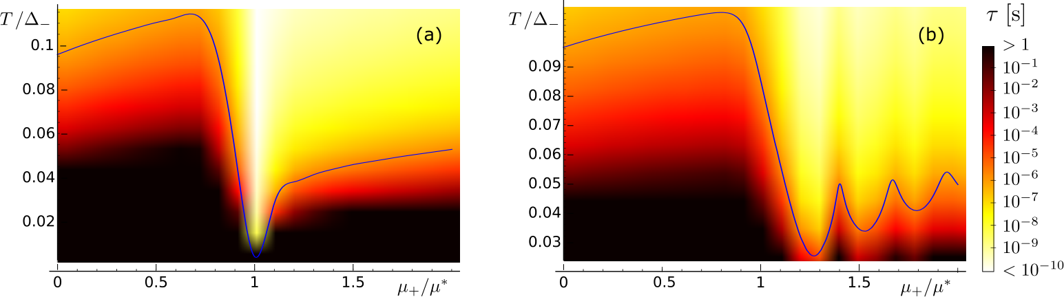
In Fig. 4 we plot $\tau$ as function of $\mu_{+}$ and $T$ and estimate the temperature $T_{\mu s}$ required to maintain the lifetime of order $1\;\mathrm{\mu}s$, i.e., $\tau(\mu_{+},T_{\mu s})=1\;\mathrm{\mu s}$. For uniform chemical potentials, $\mu_{+}=0$, the results agree with Ref. 40. For non-uniform $\mu(x)$, $\tau$ reaches its minimum if $\mu_{+}\approx\mu^{*}$. If the right section is long so that $L_{+}/\xi_{-}\gtrsim 10$ (see Fig. 4a), $T_{\mu s}$ must be as low as $\Delta_{-}/200$ at $\mu_{+}=\mu^{*}$ and in the range from $\Delta_{-}/20$ to $\Delta_{-}/10$ for larger $\mu_{+}$. If $l_{0}$ increases, the IABS energy decreases, and even lower $T_{\mu s}$’s are required at $\mu>\mu^{*}$ (see Fig. 5). Thus, if one takes $\Delta_{-}\sim 0.1-0.2\;\mathrm{meV}$ [35], $T_{\mu s}$ can be in the range $1-100\;\mathrm{mK}$ depending on $\mu_{+}$ and $l_{0}$. In order to maintain $\tau\sim 1\;\mathrm{ms}$ one has to reduce the temperature at least by a factor of two. These estimates are relevant for Majorana qubit proposals as described in Ref. 43.

For short right sections, $L_{+}\sim l_{0}\sim\xi_{-}$ (see Fig. 4b), $T_{\mu s}$ must be as low as $\Delta_{-}/50$, if $\mu_{+}$ is close to $\mu^{*}$. If $\mu_{+}$ is away from $\mu^{*}$, $T_{\mu s}\sim\Delta_{-}/30-\Delta_{-}/20$. Also, $\tau$ and $T_{\mu s}$ oscillate with $\mu_{+}$, so that a slight change in $\mu_{+}$ can lead to large variations of $\tau$ by several orders of magnitude, and fine-tuning of $\mu_{+}$ is required to maintain longer lifetimes. This situation does not occur in the qubit proposal of Ref. 43, since the trivial section located between two topological sections has to be significantly longer than $\xi_{+}$ [77]. However, it can be relevant in schemes where a gate located near the end of the NW is used to couple MBSs to a quantum dot [52, 53, 54, 55, 56, 57, 58, 51, 59]. If the gate tunes the ending of the NW out of the topological phase, $\tau$ can decrease hundreds or even thousands of times. If the right section is in the normal state with a discrete spectrum (similar to a quantum dot), the oscillations of $T_{\mu s}$ and $\tau$ are even more pronounced, and $T_{\mu s}$ can be ten times lower (see SM [73]).

We note that if one has to bring a part of the NW into the topological (trivial) phase during manipulations of MBSs or reading out a qubit, the drastical shortening of $\tau$ at $\mu\approx\mu^{*}$ can be problematic. On one hand all manipulations via gates must be adiabatically slow. On the other hand, the time span during which the local chemical potential is close to $\mu^{*}$ should not exceed the bottleneck lifetime $\tau(\mu_{+}=\mu^{*},T)$. And even if $\mu_{+}$ is significantly bigger than $\mu^{*}$, $\tau$ for a non-uniform $\mu(x)$ can be orders of magnitude shorter than in the uniform case, $\mu_{+}=0$ [40]. However, our results show that one can achieve longer lifetimes (or maintain the same $\tau$ at higher temperatures) by a better screening of the gates making the transition between the two sections more abrupt. Another option could be to increase the bulk gaps $\Delta_{\pm}$ by taking a material with larger $E_{so}$ or by tuning the tunnel-coupling to the superconductor and changing the proximity gap $\Delta_{sc}$ [78, 79, 80, 81, 82, 83, 35]. One can also optimize the gate designs and reduce the coupling constant $g$.

Conclusions.— We have studied the lifetime $\tau$ of the GS due to charge fluctuations on a nearby gate for a simple model of a topological NW with a non-uniform chemical potential. If the NW is divided into topological and trivial sections, there emerge IABSs with energies significantly below the gap. The noisy gates can excite the system from its GS to one of the IABSs reducing the lifetime of the GS. If one braids MBSs by changing gate potentials [43], the lifetime becomes extremely short if $\mu_{+}$ is close to a critical value $\mu^{*}$. Even if $\mu_{+}>\mu^{*}$ our estimations show (see Fig. 4) that $\tau$ is hundreds or even thousands times shorter than for uniform chemical potentials. In order to maintain $\tau\sim\mu s$ one has to keep the temperature below $50\;\mathrm{mK}$ if the topological gap is of order of $0.1\;\mathrm{meV}$. This estimation can also be used for short right sections, however, a fine-tuning of $\mu_{+}$ is required to achieve longer $\tau$’s. The mechanism restricting the lifetime of MBSs considered here can be dominant in comparison to the one related to the quasiparticle poisoning [38] in case of a high tunneling resistance of a barrier between the NW and the superconductor. However, if the length of the left section is of order of the correlation length $L_{-}\gtrsim\xi_{-}$, different mechanisms of the decoherence due to coupling of overlapping MBSs to electromagnetic environment or to phonons [39] may be more relevant.

This work was supported by the Swiss National Science Foundation (Switzerland) and by the NCCR QSIT. This project received funding from the European Union’s Horizon 2020 research and innovation program (ERC Starting Grant, grant agreement No 757725).

Supplemental Material for
Lifetime of Majorana qubits in Rashba nanowires with non-uniform chemical potential

References

- [1] A. Kitaev, Ann. Phys. (N. Y). 303, 2 (2003).
- [2] A. Y. Kitaev, Physics-Uspekhi 44, 131 (2001).
- [3] F. Wilczek, Nat. Phys. 5, 614 (2009).
- [4] A. Stern, Nature 464, 187 (2010).
- [5] C. Nayak, S. H. Simon, A. Stern, M. Freedman, and S. Das Sarma, Rev. Mod. Phys. 80, 1083 (2008).
- [6] A. P. Schnyder, S. Ryu, A. Furusaki, and A. W. W. Ludwig, Phys. Rev. B 78, 195125 (2008).
- [7] M. Sato and S. Fujimoto, Phys. Rev. B 79, 094504 (2009).
- [8] X.-L. Qi and S.-C. Zhang, Rev. Mod. Phys. 83, 1057 (2011).
- [9] Y. Tanaka, M. Sato, and N. Nagaosa, J. Phys. Soc. Japan 81, 011013 (2012).
- [10] S. Vijay, T. H. Hsieh, and L. Fu, Phys. Rev. X 5, 041038 (2015).
- [11] S. Vijay, and L. Fu, Phys. Rev. B 94, 235446 (2016).
- [12] J. Alicea, Phys. Rev. B 81, 125318 (2010).
- [13] R. M. Lutchyn, J. D. Sau, and S. Das Sarma, Phys. Rev. Lett. 105, 077001 (2010).
- [14] Y. Oreg, G. Refael, and F. von Oppen, Phys. Rev. Lett. 105, 177002 (2010).
- [15] V. Mourik, K. Zuo, S. M. Frolov, S. R. Plissard, E. P. A. M. Bakkers, and L. P. Kouwenhoven, Science 336, 1003 (2012).
- [16] A. Das, Y. Ronen, Y. Most, Y. Oreg, M. Heiblum, and H. Shtrikman, Nat. Phys. 8, 887 (2012).
- [17] M. T. Deng, C. L. Yu, G. Y. Huang, M. Larsson, P. Caroff, and H. Q. Xu, Nano Lett. 12, 6414 ( 2012).
- [18] D. Sticlet, C. Bena, and P. Simon, Phys. Rev. Lett. 108, 096802 (2012).
- [19] H. O. H. Churchill, V. Fatemi, K. Grove-Rasmussen, M. T. Deng, P. Caroff, H. Q. Xu, and C. M. Marcus, Phys. Rev. B 87, 241401 (2013).
- [20] L. P. Rokhinson, X. Liu, and J. K. Furdyna, Nat. Phys. 8, 795 (2012).
- [21] J. Klinovaja and D. Loss, Phys. Rev. B 86, 085408 (2012).
- [22] D. Chevallier, D. Sticlet, P. Simon, and C. Bena, Phys. Rev. B 85, 235307 (2012).
- [23] P. San-Jose, E. Prada, and R. Aguado, Phys. Rev. Lett. 108, 257001 (2012).
- [24] F. Domínguez, F. Hassler, and G. Platero, Phys. Rev. B 86, 140503 (2012).
- [25] B. M. Terhal, F. Hassler, and D. P. DiVincenzo, Phys. Rev. Lett. 108, 260504 (2012).
- [26] J. Klinovaja, P. Stano, and D. Loss, Phys. Rev. Lett. 109, 236801 (2012).
- [27] E. Prada, P. San-Jose, and R. Aguado, Phys. Rev. B 86, 180503 (2012).
- [28] W. DeGottardi, M. Thakurathi, S. Vishveshwara, and D. Sen, Phys. Rev. B 88, 165111 (2013a).
- [29] M. Thakurathi, A. A. Patel, D. Sen, and A. Dutta, Phys. Rev. B 88, 155133 (2013).
- [30] F. Maier, J. Klinovaja, and D. Loss, Phys. Rev. B 90, 195421 (2014).
- [31] S. D. Escribano, A. L. Yeyati, and E. Prada, arXiv:1712.07625
- [32] E. Prada, R. Aguado, and P. San-Jose, Phys. Rev. B 96, 085418 (2017).
- [33] A. Ptok, A. Kobiałka, and T. Domański, Phys. Rev. B 96, 195430 (2017).
- [34] A. Kobiałka and A. Ptok, arXiv:1801.08021
- [35] M. W. A. de Moor, J. D. S. Bommer, D. Xu, G. W. Winkler, A. E. Antipov, A. Bargerbos, G. Wang, N. van Loo, R. L. M. Op het Veld, S. Gazibegovic, D. Car, J. A. Logan, M. Pendharkar, J. Sue Lee, E. P. A. M. Bakkers, C. J. Palmstrøm, R. M. Lutchyn, L. P. Kouwenhoven, H. Zhang arXiv:1806.00988
- [36] J. C. Budich, S. Walter, and B. Trauzettel, Phys. Rev. B 85, 121405 (2012).
- [37] G. Goldstein and C. Chamon, Phys. Rev. B 84, 205109 (2011).
- [38] D. Rainis and D. Loss, Phys. Rev. B 85, 174533 (2012).
- [39] C. Knapp, T. Karzig, R. M. Lutchyn, and C. Nayak, Phys. Rev. B 97, 125404 (2018).
- [40] M. J. Schmidt, D. Rainis, and D. Loss, Phys. Rev. B 86, 085414 (2012).
- [41] H.-L. Lai, P.-Y. Yang, Y.-W. Huang, and W.-M. Zhang, Phys. Rev. B 97, 054508 (2018).
- [42] S. B. Kaplan, C. C. Chi, D. N. Langenberg, J. J. Chang, S. Jafarey, and D. J. Scalapino, Phys. Rev. B 14, 4854 (1976).
- [43] J. Alicea, Y. Oreg, G. Refael, F. von Oppen, and M. P. A. Fisher, Nat. Phys. 7, 412 ( 2011).
- [44] K. Flensberg, Phys. Rev. Lett. 106, 090503 ( 2011).
- [45] D. E. Liu and H. U. Baranger, Phys. Rev. B 84, 201308 (2011).
- [46] L. S. Ricco, Y. Marques, F. A. Dessotti, R. S. Machado, M. de Souza, and A. C. Seridonio, Phys. Rev. B 93, 165116 (2016).
- [47] S. Plugge, L. A. Landau, E. Sela, A. Altland, K. Flensberg, and R. Egger, Phys. Rev. B 94, 174514 ( 2016).
- [48] T. Karzig, C. Knapp, R. M. Lutchyn, P. Bonderson, M. B. Hastings, C. Nayak, J. Alicea, K. Flensberg, S. Plugge, Y. Oreg, C. M. Marcus, and M. H. Freedman, Phys. Rev. B 95, 235305 ( 2017).
- [49] L. H. Guessi, F. A. Dessotti, Y. Marques, L. S. Ricco, G. M. Pereira, P. Menegasso, M. de Souza, and A. C. Seridonio, Phys. Rev. B 96, 041114 (2017).
- [50] L. Xu, X.-Q. Li, and Q.-F. Sun, J. Phys. Condens. Matter 29, 195301 (2017).
- [51] S. Hoffman, D. Chevallier, D. Loss, and J. Klinovaja, Phys. Rev. B 96, 045440 (2017).
- [52] A. Golub, I. Kuzmenko, and Y. Avishai, Phys. Rev. Lett. 107, 176802 (2011).
- [53] B. Zocher and B. Rosenow, Phys. Rev. Lett. 111, 036802 ( 2013).
- [54] W.-J. Gong, S.-F. Zhang, Z.-C. Li, G. Yi, and Y.-S. Zheng, Phys. Rev. B 89, 245413 (2014).
- [55] M. Leijnse, New J. Phys. 16, 015029 (2014).
- [56] E. Vernek, P. H. Penteado, A. C. Seridonio, and J. C. Egues, Phys. Rev. B 89, 165314 (2014).
- [57] M. T. Deng, S. Vaitiekėnas, E. B. Hansen, J. Danon, M. Leijnse, K. Flensberg, J. Nygård, P. Krogstrup, and C. M. Marcus, Science 354, 1557 ( 2016).
- [58] D. B. Szombati, S. Nadj-Perge, D. Car, S. R. Plissard, E. P. A. M. Bakkers, and L. P. Kouwenhoven, Nat. Phys. 12, 568 (2016).
- [59] D. Chevallier, P. Szumniak, S. Hoffman, D. Loss, and J. Klinovaja, Phys. Rev. B 97, 045404 (2018).
- [60] F. L. Pedrocchi and D. P. DiVincenzo, Phys. Rev. Lett. 115, 120402 ( 2015).
- [61] D. Rainis, L. Trifunovic, J. Klinovaja, and D. Loss, Phys. Rev. B 87, 024515 (2013).
- [62] We consider only , which is a reasonable assumption for weak SOI, , while for strong SOI the results are the same for , provided is not close to the bottom of the band.
- [63] G. Kells, D. Meidan, and P. W. Brouwer, Phys. Rev. B 86, 100503 (2012).
- [64] J. Liu, A. C. Potter, K. T. Law, and P. A. Lee, Phys. Rev. Lett. 109, 267002 (2012).
- [65] D. Bagrets and A. Altland, Phys. Rev. Lett. 109, 227005 ( 2012).
- [66] P. San-Jose, J. Cayao, E. Prada, and R. Aguado, New J. Phys. 15, 075019 (2013).
- [67] D. Roy, N. Bondyopadhaya, and S. Tewari, Phys. Rev. B 88, 020502 (2013).
- [68] W. DeGottardi, D. Sen, and S. Vishveshwara, Phys. Rev. Lett. 110, 146404 (2013).
- [69] T. D. Stanescu and S. Tewari, Phys. Rev. B 89, 220507 (2014).
- [70] I. Adagideli, M. Wimmer, and A. Teker, Phys. Rev. B 89, 144506 (2014).
- [71] J. Klinovaja and D. Loss, Eur. Phys. J. B 88, 62 (2015).
- [72] C. Fleckenstein, F. Domínguez, N. T. Ziani, and B. Trauzettel, arXiv:1710.08866
- [73] See Supplemental Material at … for details concerning IABS energies. We also provide estimates for and in the regime in which the right section is normal.
- [74] C. Kittel, Introduction to Solid State Physics (Wiley, New York, 1986)
- [75] L. V. Keldysh, Sov. Phys. JETP 20, 1018 (1965).
- [76] A. Kamenev and A. Levchenko, Adv. Phys. 58, 197 (2009).
- [77] A.A. Zyuzin, D. Rainis, J. Klinovaja, and D. Loss, Phys. Rev. Lett. 111, 056802 (2013).
- [78] C. Reeg, J. Klinovaja, and D. Loss, Phys. Rev. B 96, 081301 (R) (2017).
- [79] C. Reeg, D. Loss, and J. Klinovaja, Phys. Rev. B 97, 165425 (2018).
- [80] A. E. Antipov, A. Bargerbos, G. W. Winkler, B. Bauer, E. Rossi, and R. M. Lutchyn, arXiv:1801.02616.
- [81] B. D. Woods, T. D. Stanescu, and S. D. Sarma, arXiv:1801.02630.
- [82] A. E. Mikkelsen, P. Kotetes, P. Krogstrup, and K. Flens- berg, arXiv:1801.03439.
- [83] C. Reeg, D. Loss, and J. Klinovaja, Beilstein Journal of Nanotechnology 9, 1263 (2018).
- [1] L. D. Landau, and E. M. Lifshitz, Quantum Mechanics: Non-Relativistic Theory (Pergamon Press, Oxford, 1981), 3rd Edition.
- [2] C. Ishii, Prog. Theor. Phys. 44, 1525 (1970).
- [3] O. Kulik, Sov. Phys. JETP 30, 944 (1970).
- [4] J. Bardeen and J. L. Johnson, Phys. Rev. B 5, 72 (1972).
- [5] O. Dmytruk, D. Chevallier, D. Loss, and J. Klinovaja, arXiv:1806.06842.
- [6] J. Klinovaja and D. Loss, Phys. Rev. B 86, 085408 (2012).