Stochastic receptivity analysis of boundary layer flow

Laminar-turbulent transition of fluid flows is important in many engineering applications. Predicting the point of transition requires an accurate understanding of the mechanisms that govern the physics of transitional flows. Since the 1990’s, numerical simulations with various levels of fidelity have been used to uncover many essential features of the transition phenomenon. In spite of this progress, the complicated sequence of events that leads to transition and the inherent complexity of the Navier-Stokes (NS) equations have hindered the development of practical control strategies for delaying transition in boundary layer flows [1, 2, 3].

It is generally accepted that the transition process can be divided into three stages; receptivity, instability growth, and breakdown [1]. In the laminar boundary layer flow, disturbances that lead to transition are amplified either through modal, i.e., exponential, instability mechanisms or non-modal amplification, e.g., via transient growth mechanisms such as lift-up [4, 5] and Orr mechanisms [6, 7, 8]. An important aspect in both scenarios is the receptivity of the boundary layer flow to external excitation sources, e.g., free-stream turbulence and surface roughness. Such sources of excitation perturb the velocity field and give rise to initial disturbances within the shear that can grow to critical levels. Depending on the amplitude and frequency of excitation, initial disturbances can take different routes to transition. For example, low-amplitude excitation of the boundary layer flow can cause the growth of two-dimensional Tollmien-Schlichting (TS) waves, which can trigger natural transition to turbulence [9, 10, 11, 12, 13]. On the other hand, sufficiently high levels of broad-band excitation can induce the growth of streamwise elongated streaks that play an important role in bypass transition [2]. The effect of free-stream turbulence on the growth of boundary layer streaks has been the subject of various experimental [14, 15, 16], numerical [17, 18], and theoretical [19, 20] studies. In particular, it has been shown that free-stream disturbances that penetrate into the boundary layer are elongated in the streamwise direction [21]. While nonlinear dynamical models that are based on the NS equations provide insight into receptivity mechanisms, their implementation typically involves a large number of degrees of freedom and it ultimately requires direct simulations. This motivates the development of low-complexity models that are better suited for comprehensive quantitative studies.

In recent years, increasingly accurate descriptions of coherent structures in wall-bounded shear flows, e.g. [22, 23], have inspired the development of reduced-order models. Such models are computationally tractable and can be trained to replicate statistical features that are estimated from experimentally or numerically generated data measurements. However, their data-driven nature is accompanied by a lack of robustness. Specifically, control actuation and sensing may significantly alter the identified modes which introduces nontrivial challenges for model-based control design [24]. In contrast, models that are based on the linearized NS equations are less prone to such uncertainties and are, at the same time, well-suited for analysis and synthesis using tools of modern robust control. While the nonlinear terms in the NS equations play an important role in transition to turbulence and in sustaining the turbulent state, they are conservative and, as such, they do not contribute to the transfer of energy between the mean flow and velocity fluctuations but only transfer energy between different Fourier modes [25, 26]. This feature has inspired modeling the effect of nonlinearity using additive stochastic forcing with early efforts focused on homogeneous isotropic turbulence (HIT) [27, 28, 29]. In the presence of stochastic excitation, the linearized NS equations have been used to model heat and momentum fluxes and spatio-temporal spectra in quasi-geostrophic turbulence [30, 31, 32]. Moreover, they have been used to characterize the most detrimental stochastic forcing and determine scaling laws for energy amplification at subcritical Reynolds numbers [33, 34, 35], and to replicate structural [36, 37] and statistical [38, 39] features of wall-bounded turbulent flows. In these studies, stochastic forcing has been commonly used to model the impact of exogenous excitation sources and initial conditions, or to capture the effect of nonlinearity in the NS equations.

The linearized NS equations have been widely used for modal and non-modal stability analysis of both parallel and non-parallel flows [40, 41, 42]. In parallel flows, homogeneity in the streamwise and spanwise dimensions allows for the decoupling of the governing equations across streamwise and spanwise wavenumbers via Fourier transform, which results in significant computational advantages for analysis, optimization, and control. On the other hand, in the flat-plate boundary layer, streamwise and wall-normal inhomogeneity require discretization over two spatial directions and lead to models of significantly larger sizes. Conducting modal and non-modal analyses is thus more challenging than for locally parallel flows. However, due to the slowly varying nature of the boundary layer flow, parallel flow assumptions can still provide meaningful results. For example, primary disturbances can be identified using the eigenvalue analysis of the Orr-Sommerfeld and Squire equations [41] and the secondary instabilities can be obtained via Floquet analysis [43, 12]. Moreover, the NS equations can be parabolized to account for the downstream propagating nature of waves in slowly varying flows via spatial marching. This technique has enabled the analysis of transitional boundary layers and turbulent jet flows using various forms of the unsteady boundary-region equations [44, 45], parabolized stability equations [46, 47], and the more recent one-way Euler equations [48]. Furthermore, drawing on Floquet theory, the linear parabolized stability equations have also been extended to study interactions between different modes in slowly growing boundary layer flow [49].

While the parallel flow assumption offers significant computational advantages, it does not account for the effect of the spatially evolving base flow on the stability of the boundary layer. Global stability analysis addresses this issue by accounting for the spatially varying nature of the base flow and discretizing all inhomogeneous spatial directions. Previously, tools from sparse linear algebra in conjunction with iterative schemes have been employed to analyze the eigenspectrum of the governing equations and provide insight into the dynamics of transitional flows [50, 51, 52, 53, 54]. Efforts have also been made to conduct non-modal analysis of spatially evolving flows including transient growth [55, 56] and resolvent [57, 58, 59, 60] analyses. In particular, for the flat-plate boundary layer flow, the sensitivity of singular values of the resolvent operator to base-flow modifications and subsequent effects on the TS instability mechanism and streak amplification was investigated in [57]. However, previous studies did not incorporate information regarding the spatio-temporal spectrum and spatial localization of excitation sources. The widely used resolvent analysis [61, 62, 63] is limited to monochromatic forcing, and as such, may not fully capture naturally occurring sources of excitation. Furthermore, the evolution of exact optimal perturbations that are identified using resolvent analyses is seldom encountered in practical configurations [64].

The approach advanced in the present work enables the study of receptivity mechanisms in boundary layer flows subject to stochastic sources of excitation. We model the effect of free-stream turbulence as a persistent white-in-time stochastic forcing that enters at various wall-normal locations and analyze the dynamics of velocity fluctuations around locally parallel and spatially evolving base flows using the solution to the algebraic Lyapunov equation. Our simulation-free approach enables computationally efficient assessment of the energy spectrum of spatially evolving flows, without relying on a particular form of the inflow conditions or computation of the full spectrum of the linearized dynamical generator. Moreover, the broad-band nature of our forcing model captures the aggregate effect of all time-scales without the need to integrate the frequency response over all energetically relevant frequencies.

We compare and contrast results obtained under locally parallel flow assumption with those of global analysis. Coherent structures that emerge as the response to free-stream turbulence are extracted using the modal decomposition of the steady-state velocity covariance matrix. We demonstrate how parallel and global flow analyses can be used to quantify the amplification of streamwise elongated streaks and Tollmien-Schlichting (TS) waves, which are important in the laminar-turbulent transition of boundary layer flows. Our analysis shows that subordinate eigenmodes of the steady-state velocity covariance matrices that result from global flow analyses have nearly equal energetic contributions to that of the principal modes. This observation demonstrates that global covariance matrices cannot be well-approximated by low-rank representations. On the other hand, we show how locally parallel analysis, which breaks up the receptivity process of the boundary layer flow over various streamwise length-scales, can uncover certain flow structures that are difficult to observe in global analysis. We also demonstrate that modeling the effect of free-stream turbulence using the spectrum of HIT yields similar results as the analysis based on white-in-time stochastic excitation with identity covariance matrix. For the considered range of moderate Reynolds numbers, our results support the assumption of parallel flow in the low-complexity modeling and analysis of boundary layer flows.

The remainder of this paper is organized as follows. In Section II, we introduce the stochastically forced linearized NS equations and describe the algebraic Lyapunov equation that we use to compute second-order statistics of velocity fluctuations, extract information about the energy amplification, and identify energetically dominant flow structures. In Section III, we study the receptivity to stochastic excitations of the velocity fluctuations around a locally parallel Blasius boundary layer profile. In Section IV, we extend the receptivity analysis to stochastically forced non-parallel flows. We also discuss the effect of exponentially attenuated HIT on the amplification of streaks and TS waves. In Section V, we compare the results of locally parallel and global analyses and examine the spatio-temporal frequency response of the linearized dynamics. We provide concluding remarks in Section VI.

In a flat-plate boundary layer, the linearized incompressible NS equations around the Blasius base flow profile $\bar{{\bf u}}=[\,U(x,y)\,~V(x,y)\,~0\,]^{T}$ are given by

where ${\bf v}=[\,u~v~w\,]^{T}$ is the vector of velocity fluctuations, $p$ denotes pressure fluctuations, $u$, $v$, and $w$ represent components of the fluctuating velocity field in the streamwise ($x$), wall-normal ($y$), and spanwise ($z$) directions, and ${\bf d}$ denotes an additive zero-mean stochastic body forcing. The stochastic perturbation ${\bf d}$ is used to model the effect of exogenous sources of excitation on the boundary layer flow and, as illustrated in Fig. 1, it can be introduced in various wall-normal regions. In Eqs. (II), $Re_{0}=U_{\infty}\delta_{0}/\nu$ is the Reynolds number based on the Blasius length-scale $\delta_{0}=\sqrt{\nu\,x_{0}/U_{\infty}}$, where the initial streamwise location $x_{0}$ denotes the distance from the leading edge, $U_{\infty}$ is the free-stream velocity, and $\nu$ is the kinematic viscosity. The local Reynolds number at distance $x$ to the starting position $x_{0}$ is thus given by $Re=Re_{0}\sqrt{1+x/x_{0}}.$ The velocities are non-dimensionalized by $U_{\infty}$, time by $\delta_{0}/U_{\infty}$, and pressure by $\rho U_{\infty}^{2}$, where $\rho$ is the fluid density.

We first examine the dynamics of the stochastically forced Blasius boundary layer under the locally parallel flow assumption. In this case, the base flow only depends on the wall-normal coordinate $y$ and evolution model (5) is parameterized by horizontal wavenumbers ($k_{x},k_{z}$), which significantly reduces the computational complexity. We perform an input-output analysis to quantify the energy amplification of velocity fluctuations subject to free-stream turbulence.

We compute the energy spectrum of stochastically excited parallel Blasius boundary layer flow with $Re_{0}=232$ (the Blasius length-scale is $\delta_{0}=1$). Here, we consider a wall-normal region with $L_{y}=35$ and discretize the differential operators in Eqs. (II.1) using $N_{y}=100$ Chebyshev collocation points in $y$. In the wall-normal direction, homogenous Dirichlet boundary conditions are imposed on wall-normal vorticity, $\eta(0)=\eta(L_{y})=0$ and Dirichlet/Neumann boundary conditions are imposed on wall-normal velocity, $v(0)=v(L_{y})=0$, $v_{y}(0)=v_{y}(L_{y})=0$, where $v_{y}$ denotes the derivative of $v$ with respect to $y$. In the horizontal directions, we use $50\times 51$ logarithmically spaced wavenumbers with $k_{x}\in[10^{-4},1]$ and $k_{z}\in[5\times 10^{-3},10]$ to parameterize the linearized model (5). Thus, for each pair ($k_{x},k_{z}$), the state $\mbox{\boldmath$\psi$}=[\,v^{T}\;\,\eta^{T}\,]^{T}$ is a complex-valued vector with ${2N_{y}}$ components. Grid convergence has been verified by doubling the number of points used in the discretization of the differential operators in the wall-normal coordinate.

We first consider a streamwise invariant ($h(x)=1$) solenoidal white-in-time excitation ${\bf d}$ with covariance $W=I$ in the immediate vicinity of the wall (case 1 in Table 1). Figure 3 shows largest receptivity at low streamwise wavenumbers ($k_{x}\approx 0$) with a global peak at $k_{z}\approx 0.25$. This indicates that streamwise elongated streaks are the dominant flow structures that result from persistent stochastic excitation of the boundary layer flow. Such streamwise elongated structures are reminiscent of energetically dominant streaks with spanwise wavenumbers $k_{z}\approx 0.26$ (in Blasius length-scale) that were identified in analyses of optimal disturbances [69, 70]. Slightly smaller spanwise wavenumbers have been recorded from hot-wire signal correlations in the boundary layer subject to free-stream turbulence [14]. In addition to streaks, Fig. 3 also predicts the emergence of TS waves at $k_{x}\approx 0.19$. For outer-layer forcing, the amplification of streamwise elongated structures persists while the amplification of the TS waves weakens; see Fig. 3. It is also observed that as the region of excitation moves away from the wall, energy amplification becomes weaker and the peak of the receptivity coefficient shifts to lower values of $k_{z}$. As we demonstrate in Section IV, these observations are in agreement with the global receptivity analysis of stochastically excited boundary layer flow.

As noted in Section II.2, the solution $X$ to Lyapunov equation (8) represents the steady-state (i.e., long-time average) covariance matrix of the state $\psi$ of stochastically forced linearized evolution model (5), which can be used to compute the energy spectrum in Eq. (9) or the receptivity coefficient in Eq. (14) in a simulation-free manner. To verify the values of $C_{R}$ reported in Fig. 3, we conduct stochastic simulations of the forced linearized flow equations at the wavenumber pair $(k_{x},k_{z})=(0.19,0.005)$, which is marked by the red dot in Fig. 3. This wavenumber pair allows us to examine the amplification of TS waves identified in Fig. 3. Since proper comparison with the result of the Lyapunov equation requires ensemble-averaging, rather than comparison at the level of individual stochastic simulations, we have conducted twenty simulations of system (5). The total simulation time was set to $1.6\times 10^{4}$ dimensionless time units. Figure 4 shows the time evolution of $C_{R}$ for twenty realizations of white-in-time forcing ${\bf d}$ to system (5). The receptivity coefficient averaged over all simulations is marked by the thick black line. The results indicate that the average of the sample sets asymptotically approaches the correct steady-state value of $C_{R}$.

The one-dimensional energy spectrum shown in Fig. 5 quantifies the energy amplification $E$ over various spanwise wavenumbers when forcing enters at different distances from the wall. This quantity can be computed by integrating the energy spectrum $E(k_{x},k_{z})$ (cf. Eq. (9)) over streamwise wavenumbers. In Fig. 5, the locations at which the energy spectrum peaks correspond to the spanwise scale associated with streamwise elongated streaks. When the forcing region shifts away from the wall, the energy amplification decreases, indicating that the flow region in the immediate vicinity of the wall is more susceptible to external excitation. As mentioned earlier, we also observe that, when the forcing region shifts upward, the boundary layer streaks become wider in the spanwise direction. Figure 5 shows similar trends in the receptivity coefficient as a function of spanwise wavenumber $k_{z}$, which is computed by integrating $C_{R}$ presented in Fig. 3 over streamwise wavenumbers.

The eigenvalue decomposition of the velocity covariance matrix $\Phi$ can be used to identify the energetically dominant flow structures resulting from stochastic excitation. In particular, symmetries in the wall-parallel directions can be used to express velocity components as

Here, $\mathrm{Re}$ and $\mathrm{Im}$ denote real and imaginary parts, and $\tilde{u}_{j}$, $\tilde{v}_{j}$, and $\tilde{w}_{j}$ correspond to the streamwise, wall-normal, and spanwise components of the $j$th eigenvector of the matrix $\Phi$ in Eq. (6). While all amplitudes have been normalized, the phase of these components have been modulated to ensure the compactness of $v_{j}(x,y,z)$ around $z=0$ [68]; see [38, Appendix F] for additional details.

While the sum of all eigenvalues of the matrix $\Phi$ determines the overall energy amplification reported in Fig. 5, it is also useful to examine the spatial structure of modes with dominant contribution to the energy of the flow. Figure 6 shows the contribution of the first $8$ eigenvalues of $\Phi$ to the energy amplification, $\lambda_{j}/\sum_{i}\lambda_{i}$ when the boundary layer flow is subject to stochastic forcing. For fluctuations with $(k_{x},k_{z})=(7\times 10^{-3},0.32)$ and near-wall excitation (cross in Fig. 3) the principal mode which corresponds to the largest eigenvalue, contains approximately $93\%$ of the total energy. On the other hand, for fluctuations with $(k_{x},k_{z})=(7\times 10^{-3},0.15)$ and outer-layer excitation (cross in Fig. 3) the principal mode contains approximately $52\%$ of the total energy. Figures 7 and 8 show the flow structures associated with the streamwise component of these most significant modes. From Figs. 7 and 8 it is evident that the core of streamwise elongated structures moves away from the wall with the shift of the stochastically excited region. These streamwise elongated structures are situated between counter-rotating vortical motions in the cross-stream plane (cf. Figs. 7 and 8) and contain alternating regions of fast- and slow-moving fluid, which are slightly inclined (and detached) relative to the wall. Even though these structures do not capture the full complexity of transitional flow, as we show in Section IV, they contain information about energetic streamwise elongated flow structures that are amplified by external excitation of the boundary layer flow. In particular, such alignment of counter-rotating vortices and streaks is closely related to the lift-up mechanism and the generation of streamwise elongated streaks [69, 70, 71].

The parallel flow assumption applied in Section III allows for the efficient parameterization of the governing equations over all wall-parallel wavenumbers $k_{x}$ and $k_{z}$. While this significantly reduces computational complexity, it excludes the effect of the spatially evolving base flow on the dynamics of velocity fluctuations. In global stability analysis, the NS equations are linearized around a spatially evolving Blasius boundary layer profile and the finite dimensional approximation is obtained by discretizing all inhomogeneous spatial directions. In this section, we employ global receptivity analysis to quantify the influence of stochastic excitation on the velocity fluctuations around the spatially evolving Blasius boundary layer base flow.

At any spanwise wavenumber $k_{z}$, the state $\mbox{\boldmath$\psi$}=[\,v^{T}\;\eta^{T}\,]^{T}$ of linearized evolution model (5) is a complex vector with ${2N_{x}N_{y}}$ components, where $N_{x}$ and $N_{y}$ denote the number of collocation points used to discretize the differential operators in the streamwise and wall-normal directions, respectively. While this choice of state variables is not commonly used in conventional global stability analysis of boundary layer flows, in Appendix C we demonstrate that it yields consistent results with the descriptor form in which the state is determined by all velocity and pressure fluctuations. We consider a Reynolds number $Re_{0}=232$ and a computational domain with $L_{x}=900$ and $L_{y}=35$, where the differential operators are discretized using $N_{x}=101$ and $N_{y}=50$ Chebyshev collocation points in $x$ and $y$, respectively. Similar to locally parallel analysis, we verify convergence by doubling the number of grid points.

For boundary layer flows, the global operator in Eqs. (5) has no exponentially growing eigenmodes [40]; see Remark 1. Thus, the steady-state covariance of the fluctuating velocity field can be obtained from the solution to Lyapunov equation (8) and the energy amplification can be computed using Eq. (9). As in Section III, we examine the influence of streamwise-invariant ($h(x)=1$) white-in-time stochastic forcing with covariance $W=I$ which enters at various wall-normal regions; this is achieved by filtering the forcing using the function $f(y)$ in (13). Figure 9 shows the $k_{z}$-dependence of energy amplification and receptivity coefficient for stochastic excitation entering at various wall-normal regions. Our computations show that the energy amplification increases as the region of influence for the external forcing approaches the wall, which qualitatively matches the result of the locally parallel analysis in Section III. In particular, for $Re_{0}=232$, the energy amplification reduces from $2.0\times 10^{6}$ (for stochastic excitation that enters in the vicinity of the wall (case 1 in Table 1) with $k_{z}=0.32$) to $9.6\times 10^{4}$ (for stochastic excitation that enters away from the wall (case 4 in Table 1) with $k_{z}=0.21$). Moreover, the structures that correspond to the largest energy amplification or receptivity coefficient become slightly wider in the spanwise direction, but this shift to smaller values of $k_{z}$ is not as pronounced as in parallel flows (cf. Fig. 5). The largest energy amplification and receptivity are observed for structures with $k_{z}\in[0.21,0.32]$, which is in close agreement with previous experimental [14] and theoretical studies [69, 70].

For $k_{z}=0.32$, Fig. 10 shows the contribution of the first $50$ eigenvalues of the velocity covariance matrix $\Phi$ resulting from near-wall and outer-layer stochastic excitation. In contrast to locally parallel analysis (cf. Fig. 6), we observe that other eigenvalues play a more prominent role. The implication is that in global analysis the principal eigenmode of $\Phi$ cannot capture the full complexity of the spatially evolving flow. Nevertheless, we examine the shape of such flow structures to gain insight into the effect of stochastic excitation on the eigenmodes of the covariance matrix $\Phi$ that comprise the fluctuation field. Figures 11 and 12 show the spatial structure of the streamwise component of the principal response to white-in-time stochastic forcing that enters in the vicinity of the wall and in the outer-layer, respectively. The streamwise growth of the streaks can be observed. Figures 11 and 12 display the cross-section of these streamwise elongated structures at $z=0$. As the forcing region gets detached from the wall, the cores of the streaky structures also move away from it. As shown in Figs. 11 and 12, these streaky structures are situated between counter-rotating vortical motions in the cross-stream plane and they contain alternating regions of fast- and slow-moving fluid that are slightly inclined to the wall.

We next examine the spatial structure of less energetic eigenmodes of $\Phi$. As illustrated in Fig. 10, for near-wall stochastic forcing the first six eigenmodes respectively contribute $8.9\%$, $7.3\%$, $6.1\%$, $5.3\%$, $4.6\%$, and $4.0\%$ to the total energy amplification. We again use the streamwise velocity component to study the spatial structure of the corresponding eigenmodes. As shown in Fig. 13, while the principal mode consists of a single streamwise-elongated streak, the second mode is comprised of two shorter high- and low-speed streaks. Similarly, the third and fourth modes respectively contain three and four streaks. These streaks become shorter in the streamwise direction and their energy content reduces; see Figs. 13 and 13. As the mode number increases, the streamwise extent of these structures further reduces, they appear at an earlier streamwise location, and their peak value moves closer to the leading edge. This breakup into shorter streaks for higher modes can be related to the dominant modes identified in locally parallel analysis for increasingly larger streamwise wavenumbers and at various streamwise locations (or Reynolds numbers).

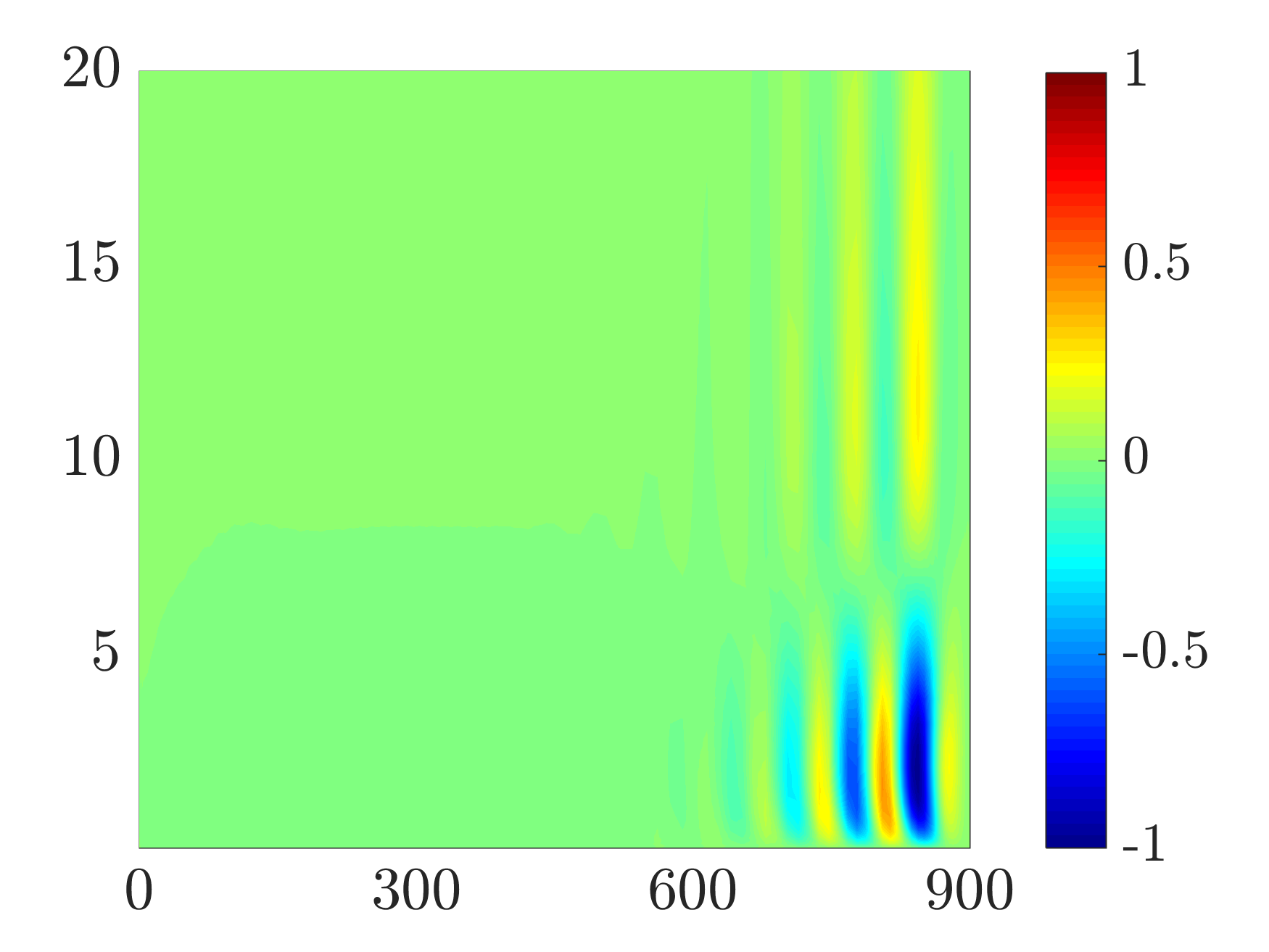
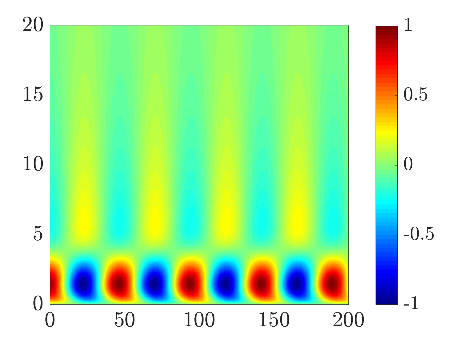
As shown in Fig. 13, spatial visualization of various eigenmodes of $\Phi$ resulting from global receptivity analysis uncovers approximately periodic flow structures in the streamwise direction. The fundamental spatial frequency extracted from the streamwise variation of the principal eigenmode of $\Phi$ provides information about the streamwise length-scales associated with the dominant flow structures. Figure 14 shows the dominant TS wave-like spatial structure that results from near-wall stochastic excitation of the boundary layer flow with $Re_{0}=232$ and $k_{z}=0.01$. The Fourier transform in the streamwise direction can be used to extract the fundamental value of $k_{x}$ associated with this spatial structure. As illustrated in Fig. 14, the Fourier coefficient peaks at $k_{x}\approx 0.1$, which corresponds to the most significant streamwise flow structures (cf. Fig. 14). The identified fundamental wavenumber is representative of the streamwise variation of this flow structure and it provides a good approximation of the dominant value of $k_{x}$ that is excited by the near-wall forcing. For different values of $k_{z}$, the filled black dots in Fig. 14 denote the streamwise wavenumbers extracted from the principal eigenmodes of the covariance matrix $\Phi$, which contribute most to the energy amplification. The circles represent the tail of streamwise wavenumbers extracted from other eigenmodes of the matrix $\Phi$. As shown in Fig. 13, for any $k_{z}$, less significant eigenmodes are associated with flow structures that are shorter in the streamwise direction. The observed trends are in close agreement with the results obtained using locally parallel analysis (cf. Fig. 3). In particular, streamwise elongated structures are most amplified for $k_{z}\approx 0.3$. On the other hand, for low spanwise wavenumbers, the TS wave-like structures are most amplified for $k_{x}\gtrsim 0.1$ (cf. $k_{x}\approx 0.19$ from locally parallel analysis).

In this section, we provide connections between the spatial flow structures obtained via locally parallel and global analyses and examine frequency responses of the boundary layer flow subject to near-wall stochastic excitation.

In the present study, we have utilized the linearized NS equations to study energy amplification in the Blasius boundary layer flow subject to white-in-time stochastic forcing entering at various wall-normal locations. The evolution of flow fluctuations is captured by two models that arise from locally parallel and global perspectives, and the amplification of persistent stochastic disturbances is studied using the algebraic Lyapunov equation. Both parallel and global flow analyses predict largest amplification of streamwise elongated streaks with similar spanwise wavelength. Moreover, TS wave-like flow structures arise from persistent near-wall stochastic excitation at long spanwise wavelengths. We have shown that as the region of excitation moves away from the wall, energy amplification reduces, which suggests that the near wall region is more sensitive to external disturbances. We have also examined the spatial structure of characteristic eddies that result from stochastic excitation of the boundary layer flow. Our computational experiments demonstrate good agreement between the results obtained from parallel and global flow models. This agreement highlights the efficacy of using parallel flow assumptions in the receptivity analysis of boundary layer flows, especially when it is desired to evaluate the energetic contribution of individual streamwise scales, which are often obscured by the dominant growth of streaks and Tollmien-Schlichting waves in global analysis.

In contrast to resolvent-mode analysis which quantifies the energy amplification from monochromatic forcing, our stochastic approach incorporates a broad-band forcing model with known spatial correlations that captures the aggregate effect of all time scales. Our Lyapunov-based framework generalizes the concept of receptivity to the amplification of velocity fluctuations from any external source of persistent excitation with known statistical properties. We note that the ability of the method to capture relevant flow physics relies on the spectral properties of the stochastic forcing that can be used to model the effect of, e.g., free-stream turbulence. In addition to white-in-time stochastic forcing with trivial (identity) spatial covariance operator, we have also investigated energy amplification arising from the streamwise-decaying forcing that corresponds to the spectrum of HIT. Our computations demonstrate close correspondence between these two case studies. The spatio-temporal spectrum of stochastic excitation sources can be further determined in order to provide statistical consistency with the results of numerical simulations or experimental measurements of the boundary layer flow [81, 39]. Implementation of such ideas to leverage statistical data and improve physics-based analysis is a topic for future research.