Adaptive Variational Particle Filtering in Non-stationary Environments

1 Introduction

Inference in online settings is challenging. It is because not only the posterior distributions should be approximated sequentially, but also one should take into account the non-stationary characteristics of the data. In these situations, suitable sequential inference procedures are required to track and bind the suitable probabilistic distance between the approximate and true posterior distribution at each time step. Otherwise the prediction errors would be propagated and leads to very poor predictions. A suitable framework for achieving online inference is online convex optimization (OCP) framework [18]. It is a sequential prediction framework with the goal to track and adapt to the environment through evaluating proper convex loss functions. By making connection between OCP and a recent efficient particle inference, we propose a particle filtering method that is suitable for online inference algorithms.

Main related works Using online convex optimization for sequential posterior approximation has been already discussed in [16,22]. However they parametrize the environment strategy space through the use of parameterized exponential family of distributions which resembles the variational inferences methodology and therefore carrying its limitations. Moreover the calculation of the loss term in [22] is not straightforward and requires other inference algorithms such as Monte Carlo Marko Chains (MCMC). Our proposed algorithm computes the loss term by reusing the generated particle. Another interesting related work to ours is [19]. It takes advantage of the mirror descent algorithm, particle methods and provides theoretical guarantees. However, 3 main key differences are: a) we address online filtering for time series data. b) unlike [19,4], our proposed online inference algorithm doesn’t have any assumption on the length of data a priori. c) Unlike [19] our proposed method follows a deterministic particle selection approach. [23] builds an online inference algorithm using particle learning (PL) method [24]. PL methods differ from sequential Monte Carlo (SMC) in that PL reverses the order of resampling and propagation procedures.

2 Preliminaries

All the vectors are denoted by bold symbols.

2.1 Online convex optimization

One way to explain the OCP framework, in the context of adversarial environments, is by considering it as a repeated game between a forecaster and an adversary. It includes the following key ingredients:

1.

Parameters of the environment $\mathbb{w}_{n}\in\Delta$ , forecaster strategies $Q(\mathbb{w}_{n})\in\mathcal{Q}$ , adversary strategies $S(\mathbb{w}_{n})\in\mathcal{S}$ .
2.

convex loss function $l(.)$ over the strategies.

3.

Shifting/Tracking Regret defined as the following minimax metric:

\displaystyle\begin{array}[]{l}\mathcal{R}_{N}^{shifting}\equiv\\ \begin{split}\displaystyle\min_{Q\in\mathcal{Q}}\max_{\mathbb{w}\in\Delta}\max_{S\in\mathcal{S}}\sum_{n=1}^{N}l(Q(\mathbb{w}_{n}))-l(S(\mathbb{w}_{n}))\end{split}\end{array}

where $N$ is the length of the sequence of observations. The forecaster’s goal is to yield the lowest total loss when played against the arbitrary sequence of adversary strategies. The goal of the OCP algorithms is to achieve sub-linearly bounded regret metric. One universal OCP algorithm is the online mirror descent algorithm MD [14]. MD casts the OCP framework to a first-order loss decrease optimization problem with Bregman distance regularizer as in Eq. 2.1:

\displaystyle\begin{array}[]{l}\begin{split}\hat{\mathbb{w}}_{n+1}=\underset{w_{n}\in\Delta}{\text{argmin}}\hskip 2.84544pt\epsilon_{n}\langle\mathbb{w}_{n},\nabla_{\mathbb{w}_{n}}l_{n}\rangle+D(\mathbb{w}_{n}\|\hat{\mathbb{w}}_{n})\end{split}\end{array}

where $\nabla_{\mathbb{w}}$ is the gradient w.r.t parameters of the environment , $\epsilon_{n}$ is the step size parameter and $D$ is the Bregman distance. Given the fixed per-observation computational complexity constraint, the MD algorithm [16] achieves the optimal shifting regret of $\sqrt{N}$ . In the section 3, we show how we can incorporate an online MD algorithm into particle filtering algorithms.

2.2 Particle Filtering

Assume a hidden Markov model (HMM) with the observations $\mathbb{y}_{N}=\{y_{1},...,y_{N}\}$ , the hidden states $\mathbb{x}_{N}=\{x_{1},...,x_{N}\}$ , $x_{n}\in\{1,...,M_{n}\}$ and $\bm{\theta}_{N}=\{\theta_{1},...,\theta_{N}\}$ as a set of parameters that controls the transition and emission processes in Eq. 6:

\begin{array}[]{l}p(x_{n},\theta_{n},y_{n}|x_{n-1},\theta_{n-1})=\\ \displaystyle p(\theta_{n})\mbox{ \begin{tabular}[t]{@{}c@{}}$\boxed{\displaystyle p(y_{n}|x_{n},\theta_{n})}$\\ \tiny emission\end{tabular}}\mbox{ \begin{tabular}[t]{@{}c@{}}$\boxed{\displaystyle p(x_{n}|x_{n-1},\theta_{n-1})}$\\ \tiny transition\end{tabular}}\end{array}

(6)

We build our framework based on flexible non-parametric models. The complexity of these models (for example the number of hidden states, etc.) increase as the amount of data grows, in a flexible manner. To this aim, an infinite capacity HMM (iHMM) model assumes that the posterior distribution of parameters $p(\bm{\theta}_{n})$ depends on the hidden states $\mathbb{x}_{n}$ and observations $\mathbb{y}_{n}$ through a low dimensional vector of sufficient statistics $c_{n}$ i.e $p(\bm{\theta}_{n}|\mathbb{x}_{n},\mathbb{y}_{n})=p(\bm{\theta}_{n}|c_{n})$ . The sufficient statistic must be updated using a deterministic recursion algorithm $\mathcal{C}$ sequentially such that $c_{n}=\mathcal{C}(c_{n-1},x_{n-1},y_{n-1})$ . The existence of such deterministic recursion as well as proper analytical integrations imply that one can marginalize out the parameters $\bm{\theta}_{N}$ from Eq. 6 as in Eq. 2.2.

\displaystyle\begin{array}[]{l}p(x_{n},y_{n}|x_{n-1},c_{n-1})=\\ \mbox{ \begin{tabular}[t]{@{}c@{}}$\boxed{\displaystyle p(y_{n}|x_{n},c_{n}=\mathcal{C}(c_{n-1},x_{n-1},y_{n-1}))}$\\ \tiny dependency between observations $y_{n}$ and $y_{n-1}$ through recursion algorithm $\mathcal{C}(.)$\end{tabular}}\\ \times p(x_{n}|x_{n-1},c_{n-1})\end{array}

¹¹ 1 For better readability, the details on the analytical integration, sufficient statistics

c_{n}

and their updating process for iHMM is moved to Appendix I.

In the filtering problems, one is interested in deriving the posterior $p(\mathbb{x}_{n+1},\mathbb{y}_{n+1})$ from $p(\mathbb{x}_{n},\mathbb{y}_{n})$ . One popular filtering approach is particle method. This especially comes in handy when the closed form expressions for the posteriors are not available. A well-known example is the sequential Monte Carlo (SMC) method [2]. In the case of generative process in Eq. 2.2, it first initializes a set of particles $\{x_{0}^{k}\}_{k=1}^{K}$ . Also for the readability of the paper, we assume that each particle encapsulates the sufficient update process $\{c_{n}^{k}=\mathcal{C}(c_{n-1}^{k},x_{n-1}^{k},y_{n-1})\}_{k=1}^{K}$ as well as the analytical integration. Therefore from now on $x_{n}^{k}$ represents $(x_{n}^{k},c_{n}^{k})$ .

It then follows these recursive steps:

1.

Propagation. Using particles $\{x_{n}^{k}\}_{k=1}^{K}$ :

$\displaystyle\begin{array}[]{l}\{W_{n}^{k}=p(y_{n},x_{n}^{k})\}_{k=1}^{K},w_{n}^{k}=\frac{W_{n}^{k}}{\sum_{j=1}^{K}W_{n}^{j}}\\ \end{array}$

$\displaystyle\begin{array}[]{l}Q(\mathbb{x}_{n},\mathbb{y}_{n})=\displaystyle\sum_{k=1}^{K}w_{n}^{k}\delta[x_{n},x_{n}^{k}]\end{array}$

where $\delta$ is Kronecker-delta.
2.

Resampling. Sample $K$ new particles with replacement $\{x_{n+1}^{k}\}_{k=1}^{K}\sim\text{Multinomial($K,w_{n}^{1},...,w_{n}^{K}$)}$

3 Mirror descent variational particle filtering

In order to reformulate the online filtering problem from an OCP perspective, we treat the environment as a posterior distribution, the strategies as the filtering strategies $Q(\mathbb{w}_{n})$ and the MC particles and their weights $\mathbb{w}_{n}=[w_{n}^{1},...,w_{n}^{K\times M_{n}}]\in\Delta^{K\times M_{n}}$ as the parameters of the environment where $M_{n}$ is the number of hidden states at sequence index $n$ and $K$ is the number of particles. Moreover the constraint of fixed per-observation computational complexity in OCP gets translated to the constraint of fixed $K$ number of particles.

Similar to [3] we builds our framework based on the Markov random field (MRF) assumption for the posterior $p(\mathbb{x}_{n},\mathbb{y}_{n})$ as in Eq. 3

\displaystyle\begin{array}[]{l}\displaystyle p(\mathbb{x}_{n},\mathbb{y}_{n})=\frac{\prod_{i=1}^{n}f(x_{i},y_{i})}{\exp(\Phi)}\end{array}

where $\Phi$ is the log-partition function and $f(x_{i},y_{i})=p(y_{i}|x_{i})p(x_{i}|x_{i-1})$ the potential function.

Algorithm 1 Mirror Descent Variational Particle Filtering (MD-VPA)

1: Input: A decreasing sequence of strictly positive discounting factors

\{\epsilon_{n}\}

, e.g

\frac{1}{n}

,

M_{0}

,

K

and initial weight vectors

\mathbb{w}_{0}=[w_{0}^{1},...,w_{0}^{K\times M_{0}}]\in\Delta^{K\times M_{0}}

2: for

n=1,2,3,...,N

do

3: for

m=1,...,M_{n}~\&~k=1,...,K

do

4:

\displaystyle\begin{split}W_{n}(k,m)=\\ \mbox{ \begin{tabular}[t]{@{}c@{}}$\boxed{\displaystyle f(x_{n}^{k}=m,y_{n})}$\\ \tiny Free energy related term\end{tabular}}\mbox{ \begin{tabular}[t]{@{}c@{}}$\boxed{\displaystyle\frac{f(x_{n}^{k}=m,y_{n+1})^{\epsilon_{n}}}{(\sum_{k=1}^{K}f(x_{n}^{k}=m,y_{n+1}))^{\frac{\epsilon_{n}}{K}}}}$\\ \tiny regret related term\end{tabular}}\end{split}

5: end for

6: Select

K

largest

W_{n}

and normalize the weights

w_{n}^{k}

for the new particles

x_{n}^{k}

.

7:

Q(\mathbb{x}_{n},\mathbb{y}_{n})=\displaystyle\sum_{k=1}^{K}w_{n}^{k}\delta[x_{n},x_{n}^{k}]

8: end for

Let’s define the loss function as the average of the predictive log-likelihood over the space of the environment space parameters $\mathbb{w}_{n}\in\Delta_{n}^{K\times M_{n}}$ as in Eq. 3:

\displaystyle\begin{array}[]{l}\begin{split}\small l_{n}(\mathbb{w}_{n})=\\ -\int_{\mathbb{w}_{n}\in\Delta_{n}^{K\times M_{n}}}\log(p(\mathbb{x}_{n},\mathbb{y}_{n}^{y_{n}\leftarrow y_{n+1}}))d\mathbb{w}_{n}\end{split}\end{array}

It is as if we were observing $y_{n+1}$ instead of $y_{n}$ and calculate the potential function $f_{n}$ with $y_{n+1}$ , given that nothing else in the history of hidden states and observation has changed. By replacing Eq. 3 in Eq. 2 and resolving a coordinate ascent algorithm leads to the proposed Mirror Descent Variational Particle Filtering (MD-VPA) described in Alg. 1. It deletes or propagates $K$ particles deterministically (out of $K\times M_{n}$ candidates living in the simplex space $\Delta^{K\times M_{n}}$ ) based on their relative contribution to the negative free energy and loss. The derivation of this coordinate-ascent algorithm is demonstrated in Appendix II. As the result of the MD prediction strategy, the following theorem is in order:

Theorem 1.

MD-VPA achieves the optimal shifting regret of $\mathcal{O}(\sqrt{N})$ for a sequence of length $N$ .

Proof.

The proof is almost the same as [16]. However [16] assumes that the set of parameters $\mathbb{w}_{n}$ are selected such that strong Hessian convexity of $\Phi(\mathbb{w}_{n})$ holds true. MD-VPA is free of this assumption. Given the finite number of particles $K$ , the deterministic nature of the particle selection process (coordinate-ascent) in MD-VPA dictates all the particles to have high probability. By noting the equivalence of the $\nabla_{\mathbb{w}_{n}}^{2}\Phi(\mathbb{w}_{n})$ with Fisher information matrix, $\mathcal{J}(\mathbb{w}_{n})=-\mathbb{E}_{\mathbb{w}_{n}}(\nabla^{2}_{\mathbb{w}_{n}}\log p(\mathbb{x}_{n},\mathbb{y}_{n}))$ then it is guaranteed that $\exists H>0,\nabla^{2}\Phi(\mathbb{w}_{n})\succeq H\mathbb{1}_{\small KM_{n}\times KM_{n}}$ . In other words, the weight of the particles are sufficiently “informative” and therefore strong Hessian convexity requirement is guaranteed. ∎

3.1 Discussion on Loss-function

Using Eq. 3 one can interpret the loss as the average predictive log-likelihood over the weight of the particles $\mathbb{w}_{n}$ . Theorem 1 then guarantees that average predictive log-likelihood stays bounded under the well-defined worst case scenarios. It achieves this by casting the variational distance as its regularizer. ²² 2 Variational distance is equivalent to Bregman distance for Markov Random Fields The variational distance however is evaluated using the $y_{n}$ rather than $y_{n+1}$ . We can evaluate it using $y_{n+1}$ instead. But one gets best filtering result when evaluating using $y_{n}$ , since this way we can incorporate the information of 2 consecutive observations in a one-pass filtering fashion. This is where the non-parametric nature of the iHMM comes to the picture where evaluating the loss (evaluated using $y_{n+1}$ ) and variational free energy (evaluated using $y_{n}$ ) in one single step is a straightforward task thanks to the existence of sufficient statistics. The idea of incorporating the loss term and MD algorithm into Bayesian Inference is mentioned in [22] as well. Their method however requires computing the loss term using the MCMC approach. The natural particle interpretation of the Alg. 1 enables it to compute the term $\mathbb{E}_{\mathbb{w}_{n}}(\log f(x_{n},y_{n+1}))=\sum_{k=1}^{K}\frac{\log f(x^{k}_{n},y_{n+1})}{K}$ by reusing the generated particle. Moreover, the sufficient statistics $c_{n}$ and the deterministic update algorithm $\mathcal{C}$ , $\{c_{n}^{k}=\mathcal{C}(c_{n-1}^{k},x_{n-1}^{k},y_{n-1})\}_{k=1}^{K}$ comes handy to compute the $\{f(x^{k}_{n},y_{n+1})\}_{k=1}^{K}$ terms easily. This makes the implementation of the MD-VPA algorithm very straightforward.

4 Simulation Results

We ran our simulations for both artificial and real data with the hyper-parameters $\alpha=\gamma=1$ . $\epsilon_{n}=\frac{1}{n}$ is set for all MD-VPA filtering algorithms. The hyper-parameters are explained in the Appendix I.

4.1 Artificial Non-Stationary Data

We first generated a sequence of 150 data using a (non-negatively correlated) HMM with 3 states and the following transition and emission matrixes respectively:

$\tiny\begin{bmatrix}0&1/2&1/2\\ 1/2&1/2&0\\ 1/2&0&1/2\end{bmatrix},\begin{bmatrix}1/2&0&1/2\\ 1/3&1/3&1/3\\ 0&1/2&1/2\end{bmatrix}$ concatanated by a negatively correlated HMM with 4 states and a multinomial emission distribution with 8 categories using the following transition and emission matrixes respectively:

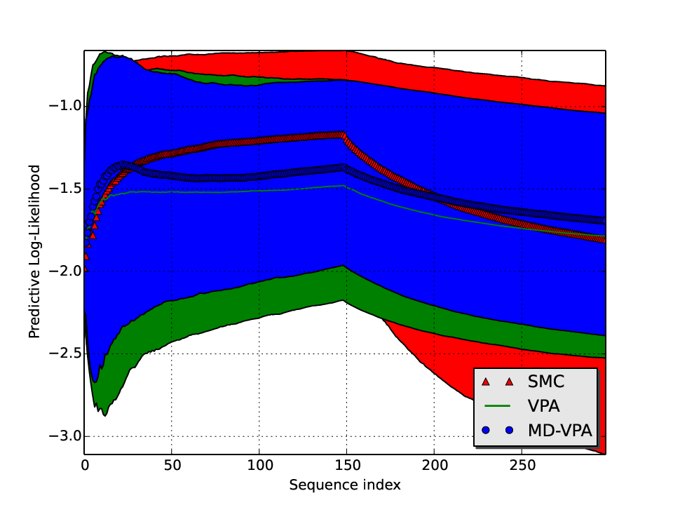
\tiny\begin{bmatrix}0&1/2&1/2&0\\ 0&0&1/2&1/2\\ 1/2&0&0&1/2\\ 1/2&1/2&0&0\end{bmatrix}

\tiny\begin{bmatrix}1/3&0&0&0&0&0&1/3&1/3\\ 1/3&1/3&1/3&0&0&0&0&0\\ 0&0&1/3&1/3&1/3&0&0&0\\ 0&0&0&0&1/3&1/3&1/3&0\end{bmatrix}

Results for $K=100$ particles are reported in Fig. 1 . We purposely generated the first half of the sequence (first 150 sequence) using a non-negatively correlated HMM with 3 states, to show that SMC performs better when less exploration in the state space is required. However as posterior gets updated, MD-VPA tracks faster and performs better than SMC and VPA in terms of both the predictive log-likelihood and the estimation variance.

Refer to caption — Figure 1: Particle filtering for changing posterior

4.2 Alice in Wonderland, Harry Potter and War and Peace

We concatenated 600 subsequent characters from beginning of “Alice in Wonderland”, 600 from “Harry Potter” and 600 from “War and Peace”. The results are shown in Fig. 2 for 50 particle and 50 random initial states. MDA outperforms SMC and VPA in terms of both the predictive log-likelihood and the estimation variance.

4.3 Web-Click

MD-VPA performs exceptionally good when it gets applied to the MSNBC.com Web Data Set [26]. It contains sequential categorical data collected from news-related portions of msn.com. Each sequence in the dataset corresponds to page views of a user. Each event in the sequence corresponds to a user’s request for a page. Requests are recorded at the level of page category. It is natural that different users have different interests for visiting pages. Therefore data contains arbitrary sequences of users’ web-hopping strategies. The results are shown in Fig. 3 with 100 particles. We have avoided plotting the estimation error as we observed no considerable difference between the compared algorithms.

5 Conclusion

The main novelty of our work is to address the efficient particle inference for non-stationary sequential data from the perspective of online convex optimization approaches. MD-VPA is implemented for iHMM modeling of the artificially generated data as well as the text and web data. It approximates and tracks the change in the posterior faster and more efficiently compared with other filtering mechanisms. One interesting future work is to compare MD-VPA against adversarial environments. Strong links between the particle filtering methods and problem of sequential lossless coding can be established using our work and the results in [16,20]. For example, the particle efficiency concept in the online particle filtering methods can be mapped to the concept of code redundancy in the sequential lossless coding. An interesting future work can be examining these connections in more details.

6 REFERENCES

[1] Wainwright,M. J. & M. I. Jordan. (2008) Graphical models, exponential families, and variational inference. Foundations and Trends in Machine Learning, 1(1-2), pp. 1–305.

[2] Doucet, A., De Freitas, N., Gordon, N., et al. (2001). Sequential Monte Carlo methods in practice. New York: Springer Press.

[3] Saeedi, A, Kulkarni, T.D, Mansinghka, V & Gershman. (2015) S. Variational particle approximations . arXiv:1402.5715v3

[4] Hoffman, M, Blei, D.M , Paisley, J & Wang. C. (2013) Stochastic variational inference. Journal of Machine Learning Research, 14. pp. 1303–1347.

[5] Broderick, T, Boyd, N, Wibisono, A, Wilson, AC, & Jordan, M. (2013) Streaming variational Bayes. Advances in Neural Information Processing Systems.

[6] Honkela, A & Valpola, H. On-line variational Bayesian learning. (2003) it In 4th International Symposium on Independent Component Analysis and Blind Signal Separation. pp. 803–808.

[7] Tank, A, Foti, N & Fox, E. (2015)Streaming variational inference for Bayesian nonparametric mixture models. In International Conference on Artificial Intelligence and Statistics.

[8] Theis, L & Hoffman, M.D. (2015) A trust-region method for stochastic variational inference with applications to streaming data. arXiv preprint arXiv:1505.07649.

[9] Ahmed, A, Ho, Q, Teo, C.H, Eisenstein, J, Xing, E.P & Smola, A.J. (2011) Online inference for the infinite topic-cluster model: Storylines from streaming text. In International Conference on Artificial Intelligence and Statistics. pp. 101–109.

[10] Yao, L , Mimno, D & McCallum, A. (2009) Efficient methods for topic model inference on streaming document collections. In ACM Conference on Knowledge Discovery and Data Mining. pp. 937–946.

[11] Doucet, A, Godsill, S & Andrieu, C. (2000) On sequential MonteCarlo sampling methods for Bayesian filtering. Statistics and Computing, 10(3). pp. 197–208.

[12] Gal, Y & Ghahramani, Z. (2014). Pitfalls in the use of Parallel Inference for the Dirichlet Process. Proceedings of the 31st International Conference on Machine Learning

[13] Teh, Y. W., Jordan, M. I., Beal, M. J., & Blei, D. M. (2006). Hierarchical Dirichlet processes. Journal of the american statistical association.

[14] Srebro, N, Sridharan, K & Tewari, A. (2011) On the Universality of Online Mirror Descent . Advances in Neural Information Processing Systems 24.

[15] Matthew J. Beal, Zoubin Ghahramani and Carl Edward Rasmussen, (2001). The Infinite Hidden Markov Model, Advances in Neural Information Processing Systems 14).

[16] Raginsky, M, Willett, R.M, Horn, C, Silva, J & Marcia, R.F (2012). Sequential anomaly detection in the presence of noise and limited feedback. IEEE Transactions onInformation Theory Vol. 58. pp. 5544–5562.

[17] Krichevsky R. E. & Trofimov V. K. (1981). The performance of universal encoding. IEEE Trans. Inform. Theory, vol. IT-27, no. 2. pp. 199–207.

[18] Cesa-Bianchi, N & Lugosi, G. (2006)Prediction, learning, and games. Cambridge University Press.

[19] Bo Dai, Niao He, Hanjun Dai and Le Song (2016). Provable Bayesian Inference via Particle Mirror Descent. 19th International Conference on Artificial Intelligence and Statistics. pp. 985?994.

[20] Shamir, G. I., & Merhav, N. (1999). Low-complexity sequential lossless coding for piecewise-stationary memoryless sources. Information Theory, IEEE Transactions on, 45(5). pp. 1498–1519.

[21] Bo Dai, Niao He, Hanjun Dai and Le Song, Provable Bayesian Inference via Particle Mirror Descent, The 19th International Conference on Artificial Intelligence and Statistics, 2016.

[22] Guhaniyogi, R., Willett, R. M., & Dunson, D. B. (2013). Approximated Bayesian Inference for Massive Streaming Data Duke Discussion Paper.

[23] A. Rodriguez, (2011). Online learning for the infinite hidden Markov model. Communications in Statistics - Simulation and Computation 40 (6). pp. 879-893.

[24] Carlos M. Carvalho, Hedibert F. Lopes, Nicholas G. Polson, and Matt A. Taddy. (2010). Particle learning for general mixtures. Bayesian Anal Vol. 5. pp. 709-740.

[25] Van Gael, J., Saatci, Y., Teh. & Ghahramani , Z. (2008). Beam sampling for the infinite hidden Markov model. In Proceedings of the 25th International Conference on Machine Learning (ICML).

[26] MSNBC-WebData

7 Appendix I

The sufficient statistics are $c_{n}=(M_{n},\{t_{jc}\})$ where $M_{n}$ is the number of distinct hidden states up to the time $n$ and $\{t_{jc}\}$ is the number of transitions between states $j$ and $c$ up to time $n$ .

The analytical integrations is according to the Chinese restaurant franchise in [13]. $x_{n}$ is assigned to state $c$ with probability proportional to $t_{x_{n-1}c}$ or to a state never visited from $x_{n-1}$ , ( $t_{x_{n-1}c}=0$ ) with probability proportional to $\alpha$ . If an unvisited state is selected, $x_{n}$ is assigned to state $c$ with probability proportional to $\sum_{j}t_{jc}$ , or a new state (i.e, one never visited from any state, $\sum_{j}t_{ic}=0)$ with probability proportional to $\gamma$ . The parameters $\alpha,\gamma$ are the hyper parameters for the iHMM.

The sufficient statistic updating process $\mathcal{C}_{n}$ is then simply the book keeping of the number of counts $\{t_{jc}\}$ and updating them at each time $n$ recursively.

8 Appendix II

The goal is to solve the Eq. 2.1. First note that Variational distance is equivalent to Bregman distance for Markov Random Fields. The using the following relation, we instead maximize negative free energy $\mathcal{L}(\mathcal{Q})$ .

\displaystyle\begin{array}[]{l}\Phi=KL[\mathcal{Q}\|p]+\mathcal{L}[\mathcal{Q}]\end{array}

where $KL[\mathcal{Q}\|p]=\sum_{\mathbb{x}_{n}}\mathcal{Q}(\mathbb{x}_{n},\mathbb{y}_{n})\log\frac{\mathcal{Q}(\mathbb{x}_{n},\mathbb{y}_{n})}{p(\mathbb{x}_{n},\mathbb{y}_{n})}$ and

\displaystyle\begin{array}[]{l}\mathcal{L}(\mathcal{Q})=\sum_{\mathbb{x}_{n}}\sum_{i=1}^{n}\mathcal{Q}(\mathbb{x}_{n},\mathbb{y}_{n})\log\frac{f(x_{i},y_{i})}{\mathcal{Q}(\mathbb{x}_{n},\mathbb{y}_{n})}\end{array}

Using Eq. 1, one can parametrize $\mathcal{Q}$ and in turn the negative free energy term $\mathcal{L}(\mathcal{Q})$ as follows:

\displaystyle\begin{array}[]{l}\begin{split}\mathcal{L}[\mathbb{w}_{n}]=\sum_{k=1}^{K\times M_{n}}w_{n}^{k}\log\frac{f(x_{n}^{k},y_{n})}{w_{n}^{k}V_{n}^{k}}\end{split}\end{array}

Moreover we want to use only $K$ particles (fixed per-observation computational complexity). This introduces the constraint $\sum_{k=1}^{K}w_{n}^{k}=1$ . With this constraint being added as a Lagrange multiplier $\lambda$ to the Eq. 3, and substituting for $\mathcal{L}[\mathbb{w}_{n}]$ using Eq. 8, we end up with the following formulation:

\displaystyle\begin{array}[]{l}\begin{split}\mathbb{w}_{n+1}=\underset{\mathbb{w}_{n}\in\Delta^{K\times M_{n}}}{\text{argmax}}\hskip 2.84544pt-\epsilon_{n}\langle\mathbb{w}_{n},\nabla_{\mathbb{w}_{n}}l_{n}\rangle+\\ \mathcal{L}[\mathbb{w}_{n}]+\lambda(\sum_{k=1}^{K}\mathbb{w}_{n}^{k}-1)\end{split}\end{array}

Noting that derivatives of log-partition function $\nabla_{\mathbb{w}_{n}}(\Phi(\mathbb{w}_{n}))=[\mathbb{E}_{w^{1}}(\log f),...,\mathbb{E}_{w^{K\times M_{n}}}(\log f)]$ and taking derivative w.r.t $w_{n}^{k}$ and equating to zero we obtain:

\displaystyle\begin{array}[]{l}\log f(x_{n}^{k},y_{n})-\log w_{n}^{k}-\log V_{n}^{k}+\lambda-1\\ +\epsilon_{n}\log f(x_{n}^{k},y_{n+1})-\epsilon_{n}\mathbb{E}_{w_{n}^{k}}(\log f(x_{n},y_{n+1}))=0\implies\\ \noindent w_{n+1}^{k}=\frac{Z_{w_{n}}^{-1}f(x_{n}^{k},y_{n})f(x_{n}^{k},y_{n+1})^{\epsilon_{n}}}{\exp(\epsilon_{n}\mathbb{E}_{w^{k}_{n}}(\log f(x_{n},y_{n+1})))V^{k}}\end{array}

, where

\displaystyle\begin{array}[]{l}\begin{split}Z_{w_{n}}=\exp(\lambda-1)^{-1}=\\ \sum_{k=1}^{K}\frac{f_{n}(x_{n}^{k},y_{n})f(x_{n}^{k},y_{n+1})^{\epsilon_{n}}}{\exp(\epsilon_{n}\mathbb{E}_{w_{n}^{k}}(\log f(x_{n},y_{n+1})))V_{n}^{k}}\end{split}\end{array}

Moreover the Hessian convexity $\nabla_{\mathbb{w}_{n}}^{2}\Phi(\mathbb{w}_{n})\succ 0$ implies the concavity of the maximization problem and therefore existence of a solution can be confirmed. By computing $\mathbb{E}_{w_{n}}(\log f(x_{n},y_{n+1}))=\sum_{k=1}^{K}\frac{\log f(x^{k}_{n},y_{n+1})}{K}$ and replacing it in Eq. 8, we end up with Algorithm 1.