[CCTP-2018-3, ITCP-IPP 2017/22]
Elasticity bounds from Effective Field Theory
Abstract
Phonons in solid materials can be understood as the Goldstone bosons of the spontaneously broken spacetime symmetries. As such their low energy dynamics are greatly constrained and can be captured by standard effective field theory (EFT) methods. In particular, knowledge of the nonlinear stress-strain curves completely fixes the full effective Lagrangian at leading order in derivatives. We attempt to illustrate the potential of effective methods focusing on the so-called hyperelastic materials, which allow large elastic deformations. We find that the self-consistency of the EFT imposes a number of bounds on physical quantities, mainly on the maximum strain and maximum stress that can be supported by the medium. In particular, for stress-strain relations that at large deformations are characterized by a power-law behaviour , the maximum strain exhibits a sharp correlation with the exponent .
pacs
Valid PACS appear hereI Introduction
A prominent and early example of an Effective Field Theory (EFT) is the theory of elasticity: the continuum-limit description of a solid’s mechanical response, including its sound wave excitations – the phonons [1, 2].
As in hydrodynamics, elasticity theory can be phrased as a derivative expansion for an effective degree of freedom – the displacement vector of the solid elements with respect to equilibrium. Importantly, the classic elasticity theory can be promoted to the nonlinear regime, addressing the response to finite deformations [3, 4, 5]. Operationally, this is done by finding the stress-strain relations for both finite shear or bulk strain applied to the material. These diagrams encode several response parameters (such as the proportional limit or the failure point, see [5] for definitions), which are well defined material properties that go deep into the nonlinear response regime. Typically, these parameters are difficult to compute from the microscopic constituents, so there is a chance that EFT methods may help in understanding some nonlinear elasticity phenomena.
From the viewpoint of quantum field theory (QFT), it is clear that elasticity theory can be treated as a non-trivial (i.e., interacting) EFT. The way how this theory works as an EFT, however, is quite different from other well known examples, mostly because the underlying symmetry breaking pattern involves spacetime symmetries.
The purpose of this work is to revisit finite elasticity theory from the viewpoint of QFT. We aim at clarifying how the EFT methodology works for broken spacetime symmetries and find novel relations between (and bounds on) various nonlinear elasticity parameters.
II From Goldstones to stress-strain curves
We start by stating the precise QFT sense in which elasticity theory can be treated as an EFT. The first requirement is that the material must have a separation of scales: we shall consider only low frequency (acoustic) phonons; any other mode is considered as much heavier and integrated-out. (Materials displaying scale invariance violate this assumption and deserve a separate treatment.) Under this condition we can exploit the fact that the phonons can be viewed as the Goldstone bosons of translational symmetry breaking [6, 7, 8]. As such we obtain their fully nonlinear effective action by the means of the standard coset construction [9].
For simplicity, we shall work in spacetime dimensions, where the dynamical degrees of freedom are contained in two scalar fields .
The internal symmetry group is assumed to be the two-dimensional Euclidean group, , acting like translations and rotations in the scalar fields space. The theory then must be shift invariant in the ’s implying that any field configuration that is linear in the spacetime coordinates will satisfy the equations of motion. The equilibrium configuration of an isotropic material is given by:
| (1) |
This vacuum expectation value spontaneously breaks the symmetry group down to the diagonal subgroup.
Following the coset construction method, one concludes that the effective action at lowest order in derivatives takes the form
| (2) |
with and defined in terms of the scalar fields matrix11 1 We retain the curved spacetime metric only to make it clear how the energy-momentum tensor arises from this action. In practice we shall always work on the Minkowski background . as . The function is ‘free’ and its form depends on the solid. In this language, the phonons are identified as the small excitations around the equilibrium configuration defined through . Plugging this decomposition into (2) one can find the phonon kinetic terms and their self-interactions . The leading phonon effective operators are determined by a few Wilson coefficients that are related to the lowest derivatives of evaluated on the equilibrium configuration, see [10] for details. (Analogous results can be found in [11] for superconductors.) The effective action (2) also encodes the response to finite (large) deformations, and for that the global form of is needed.
By symmetry considerations one cannot restrict the action (2) any further.
To identify what is the function for a given material one needs more information, some kind of constitutive relation. According to the finite elasticity literature (see e.g., [5]) the function is naturally identified with the so-called strain-energy function.
This is a function of the principal invariants characterizing the materials state of deformation. It encodes the full nonlinear response for the so-called Cauchy hyperelastic solids, for which plastic and dissipative effects can be ignored [4].
The form of can then be found from the stress-strain relations measured in both the shear and the bulk channels of real solids (see, e.g. [4, 3, 12]). More specifically, from the response of the material to constant and homogeneous deformations. These can be reduced to configurations of the form
| (3) |
where and are the shear and the bulk strains respectively, and they induce constant but non-trivial values of and . The amount of stress in the material generated by (or needed to support) such a configuration depends only on the strains , and on the shape of , see e.g. Eq. (9). The upshot is that it is possible to reconstruct the full form of the effective Lagrangian (up to an irrelevant overall constant) by just measuring the stress-strain relations, that is, from the response to time-independent and homogeneous deformations. This already illustrates how the solid EFTs retain predictive power.
The next apparent challenge from the QFT viewpoint is that the real world stress-strain curves typically exhibit a dramatic feature: they terminate at some point, corresponding to the breaking (or elastic failure) of the material. It is then natural to ask how exactly is the breaking seen in the EFT. Must the function be singular? Or does the breaking correspond to a dynamical process (e.g., an instability) that can be captured within the EFT with a regular ? We argue below that the latter possibility can certainly arise allowing to extract relations between the parameters that control the large deformations.
The main task then is to analyze the stability properties of the strained configuration (3). This can be done by setting in (2) and expanding for ‘small’ . In doing so one easily finds that the phonon sound speeds depend on the applied strain . This is a long known phenomenon, the acoustoelastic effect, see e.g. [13, 14, 15, 16, 17, 18]. Still, we argue here that this can have a great impact on the stress-strain relations, eventually limiting the maximal stress that a material can withstand. The reason is that generically, increasing the strain results into increasing/decreasing the various sound speeds – typically in an unbounded fashion. In particular, in most cases past some large enough strain value, , one of the sound speeds becomes either imaginary or superluminal. Case implies that the material develops an instability and it must evolve to a different ground state. Case prevents the existence of a Lorentz invariant ultraviolate completion. Therefore the effective low energy description (2) must be physically invalid at least for such a large deformation. In any case, one can translate the constraints and as upper bounds on the maximum allowed strain that is compatible with the given choice of . We remark that these bounds arise even for smooth choices of the effective Lagrangian , and yet they naturally lead to stress-strain curves that terminate at some point , see Fig. 1 for some illustrative examples.
Additionally, demanding that none of these pathologies occur for materials that we know admit large deformations (elastomers) significantly constrains the stress-strain curves and therefore the possible nonlinear response of materials on quite general grounds. We illustrate the point by focusing on materials/EFTs which allow for large deformations and which realize stress-strain curves with a power-law scaling
| (4) |
Henceforth we shall refer to as the strain exponent. As we show below, both the maximum strain and the exponent are bounded from above, and there is a general relation between the two. It is unclear to us to what extent these results were already known before. Nonetheless, our main goal is to show how the EFT perspective presented here brings some additional layer of understanding to these phenomena.
Firstly, let us obtain the corresponding stress-energy tensor by varying the action with respect to the curved spacetime metric and evaluating it on the Minkowski background, :
| (5) |
For any time independent scalar field configurations, the stress-energy tensor components are
| (6) | ||||
| (7) | ||||
| (8) |
where etc. Henceforth we shall work with the deformed field configuration (3) which, introduces both shear and bulk deformation. In particular, when setting , it describes a pure shear strain (i.e. volume-preserving) in the directions induced by . For and , the same setup encodes a pure bulk strain. In the considered scalar field background configuration and take the values: .
In particular, the full nonlinear stress-strain curve for pure shear deformations as a function of reads:
| (9) |
The analogous stress-strain curve for pure bulk deformations can also be found by expressing as a function of the bulk strain, . It is thus clear that from the knowledge (measurement) of both shear and bulk diagrams one can extract the shape of – the full effective Lagrangian. For instance, under the assumption that the dependence is negligible, then from a given shear stress-strain curve one can extract
To make the connection to the linear elasticity theory explicit one considers small shear and bulk deformations i.e. small values of and . Then, as usual, elastic deformations at linear level are described in terms of the displacement tensor
| (10) |
where is the displacement away from the equilibrium state, . A deformation of the body that changes its volume is given by the compression or bulk strain as . In turn, a deformation that only affects its shape – pure shear – is given by .
Expanding both the stress-energy tensor components (7), (8) and the displacement tensor (10) up to linear order in and one recovers the usual expression in 2+1 dimensions:
| (11) |
where is the equilibrium pressure and are the shear and bulk elastic moduli. In the case of a pure shear deformation this gives and we can read off the shear modulus as
| (12) |
Similarly for the case of pure bulk strain () we first note that the equation (7) holds at nonlinear level, i.e. for arbitrarily large values of . In order to find the linear bulk modulus we expand both the bulk strain and the bulk stress around the equilibrium value . For the stress this gives with the equilibrium pressure given in (7) and . The bulk modulus is then:
| (13) |
where all the quantities are evaluated at .
All the details concerning the consistency and stability of perturbations around the strained background configuration are given in Appendix A. There we find that the spectrum of perturbations contains two gapless phonon modes
| (14) |
with the sound speeds bearing a nonlinear dependence on the strain parameters . For the consistency and stability of a given around the background (3) we require the absence of: modes with negative kinetic energy, i.e. ghosts; negative sound speeds squared, i.e. gradient instability; superluminal propagation. In each case this leads to a certain value of maximal strain, , beyond which one of these consistency conditions is violated. A typical stress-strain curve exhibiting this behavior, obtained for a given choice of , is shown in Fig. 1.
It is important to remark that our expressions for derived in Appendix A should be interpreted as giving an upper bound on the maximum strain that the material can support, since other effects not included here can enter before, thus lowering the actual maximum . For instance, one expects plastic/dissipative effects to enter at some point in real materials. However, this alters our analysis only for , thus we still obtain an upper bound on the maximum reversible deformability.
It is interesting to consider the possibility that it really is the found here (or a value very close to it) that corresponds to the physical limitation to the material deformation. In this case, the EFT gives partial information on how the material might ‘break’. As was mentioned earlier, there are two main options: that the breakdown is due to gradient instability or due to reaching superluminality.
In the case of gradient instability one expects that, like any instability, this is physically resolved by a transition to another ground state, most likely described by a different EFT. The specific nature of this transition remains hidden in the leading order low energy EFT presented in this work. For instance, whether the gradient instability develops as a soft (slow) or hard (fast) process depends on the nature of the next-to-leading order corrections to . One may speculate that the hard case corresponds to a breaking of the material and the soft case to the necking phenomenon – a decrease in the cross-sectional area of a material sample that is often seen under tensile stress. This would resemble the so-called ‘soft phonon’ instability observed in some materials, see [19, 20, 21, 22, 23, 24, 25, 26].
Concerning superluminality, let us emphasize that in contrast to ghost and gradient instabilities the issue of superluminal propagation relates to the possibility of a Lorentz invariant UV completion, not to the stability of propagation [27]. In order to apprehend the physical picture, it is instructive to recall a classic in field theory: the example given by high spin fields where the problem of superluminality is known to arise [28]. As discussed in [29, 30], there are two ways to resolve the problem, which require to augment the EFT either by higher order operators or with additional light degrees of freedom. Any of the two resolutions makes it manifest that the naive EFT truncation (akin to the one that we are doing in Eq. (2)) breaks down. Moreover, it also gives an idea of how – what that truncation might be missing. In our case, this means that in the vicinity of violating the no-superluminality condition, corrections to the particular shape of that we consider must become important either by the presence of additional operators or light fields. The possibility that higher order operators (with more derivatives) can fix the superluminality problem while keeping the rest of the elastic response properties is nontrivial and we leave it for future research. On the other hand, the possibility that one needs to supplement the benchmark model with other light degrees of freedom seems quite reasonable – after all in real world materials phonons do couple to many other modes. If this is the resolution, then the physical interpretation of the bound given by superluminality is that can be understood as an upper limit on when these light degrees of freedom have to be taken into account.
III Results in a scaling model
For concreteness we shall focus on the simple potential
| (15) |
where is the dimensionful energy density set by the equilibrium configuration. The reason for choosing this form is that it realizes a power-law scaling like (4) at large deformations, . This behavior is observed in hyperelastic rubber-like materials, and there are many phenomenological models [4, 12, 31, 32, 33, 34, 35, 36] that reduce to (15) at large strains with various strain exponents . Here we are interested in characterizing how the stress-strain curves (and mainly the maximum stress and strain) depend on the parameters . Let us also note that there are two special ‘corners’ in parameter space: for the benchmark potential describes a perfect fluid [7, 9]; for , the model reduces to two free scalar fields.
We first find that the linear elastic moduli for the potential (15) take the simple form
| (16) |
They are both positive for , . Moreover the Poisson’s ratio – the negative ratio of transverse to axial strain – for our models as [37] is readily obtained as:
| (17) |

The result is shown in Fig. 2. At large the ratio is close to its upper bound meaning that the models are close to perfect incompressible elastic materials. At small values of and large the ratio tends to its lower negative bound. A negative Poisson’s ratio is typical of more exotic (the so-called auxetic) materials like some foams and metamaterials. Interestingly, the limit of free canonical scalars is in that regime. Finally, for most of the models described, , as is common for steels and rigid polymers.
For the full nonlinear response to pure shear, Eq. (9) gives:
| (18) |
This is shown in Fig. 1 for various values of and . Notably, the stress-strain curves obtained from the benchmark models mimic a large variety of materials including fibers, glasses and elastomers [12]. More precisely, Eq. (18) describes Neo-Hookean systems which follow Hooke’s law at small strain but exhibit non-linear power-law scalings at large deformations [5]. Similarly, the nonlinear response to a pure compression, that we define as , reads
| (19) |
We show the full nonlinear response to pure bulk deformation for various values of in Fig. 3.
As per construction, at large strains, , the nonlinear stresses display power-law scalings of the form:
| (20) |
from where we read off the shear and bulk strain exponents as: and . Note that, as can be seen from Eq. (16), and also control the linear shear and bulk moduli.
Combining the requirements of the absence of ghosts, gradient instabilities and superluminal propagation with the positivity of the elastic moduli, and , constrains the allowed range of parameters. In the simple case of linear deformations we obtain the following allowed region for the exponents :
| (21) |
The analysis can be extended to finite strain and as mentioned above leads us to another important result: the existence of a maximum strain that can be supported by the system before the onset of one of the aforementioned pathologies. How depends on the strain exponents is shown in Fig.4; the exact analytic expressions can be found in the Appendix.22 2 Let us remark that, as can be inferred from Eq. (18), the power-law scaling can really be reached only for . Therefore, the limits shown in Fig. 4 can only be extended to a material following (20) at large strains in the bluish part of the diagram. We must emphasize that the obtained in this way is not meant to be the actual maximum deformation that a material with the aforementioned scaling properties can withstand, but rather an upper bound on it. Still, this already provides quite a lot of information. For instance, in the large (yellowish) area of Fig. 4 where only reaches values of , one can already discard the existence of very elastic materials that exhibit scaling as in (4) with those scaling exponents.
We note that the regions in the parameter space where large strains can be supported are near the special points (free scalars) or (fluid limit). Therefore, for the model (15), we expect the real-world (non-relativistic) solids to lie near the axis. In this limit, the maximum strain is set from the absence of gradient instability for almost all values of .
Intriguingly, for a number of ‘universal’ correlations appear. First, we find a universal scaling of the maximum strain
| (22) |
Inserting this in the expression (9) for the nonlinear shear stress we further obtain
| (23) |
This shows a linear dependence of the maximal stress supported by a material on the strain exponent , which in our simple model controls also the linear elastic modulus. Similar linear correlations are observed experimentally in various materials [38, 39, 40, 41, 42]. Additionally, we also find a clear relation between the hardness and the maximum strain, . Let us emphasize, however, that whether the correlations that we find can be extrapolated to real world materials strongly depends on whether their stress-energy function behaves as a power law at large strain, and whether they can support large deformations.

Finally, let us note that within the benchmark model (15) there are no constraints on the bulk strain arising from the consistency and stability requirements. This is a consequence of (15) being a monomial. For more general choices, additional bounds can arise. Let us also mention that for it is possible to achieve a negative bulk modulus, , in a way that is perfectly consistent from the EFT perspective. In particular, as long as the stability constraint is still satisfied. This has also been studied in four dimensions [43, 44] and observed experimentally [45].
IV Non-relativistic solids
The benchmark model Eq. (15) considered above has been useful to exhibit the constraining power of the EFT methods, however it has one disadvantage: the region in parameter space giving small sound speeds as in real-world elastic materials is very small. To be more specific, the typical sound speeds are at most of order in the units of the speed of light. In the parameter space , this corresponds to the corner where both and are of order , or less. The problem with this is that in the benchmark model (15) and also control the exponents in the stress-strain relation at large strain, with for pure shear and for pure bulk deformations respectively. It follows that the benchmark models can only cover realistic materials with very specific exponents, basically and . Clearly, there has to be a way around this limitation because elastic materials with more generic values for do exist and one expects that a similar EFT construction should describe them. The obvious guess is that the benchmark choice Eq. (15) is too restrictive. In this section we show how to deform the model in order to have small speeds of sound while keeping large deformability and generic exponents.
Fortunately, there is a well motivated and unique way to ensure that the sound speeds become as small as needed while preserving the stress-strain relations untouched. This is achieved by adding an extra term to the potential with a large coefficient in front. This term is special for many reasons. Physically, it is proportional to the mass density of the material [6]. This immediately explains why the coefficient in front of it must be large in the non-relativistic materials. The mass density contributes to the Lagrangian (an energy density) weighted by [6] and is much larger than the typical stresses in solids. Related to this, in the fluctuations around any background, this term only produces temporal kinetic terms, as can be easily seen in equations (32)-(37) in Appendix A, noting that this term satisfies . Therefore, this new term only contributes to the denominators in the formulas for the speeds, and so enhancing it decreases the speeds.
Moreover, an important feature of this term is that it does not affect neither the bulk stress nor the shear stress , so it doesn’t alter the stress-strain relations (this is clear from Eqs. (7) and (9)). This term only appears in the energy density , as it must be, since it only accounts for the inertial mass and thus it contributes like ‘dust’ (pressureless fluid). This is crucial to retain the predictive/constraining power of the EFT framework, because in order to go to the non-relativistic regime it suffices to add one single parameter in the full nonlinear Lagrangian.
For these reasons, it suffices to switch to the following model,
| (24) |
with a small parameter (which is a measure of the typical speeds in the units of the speed of light). This guarantees that the material is non-relativistic while keeping the nonlinear static elastic response the same as in the benchmark model (15).
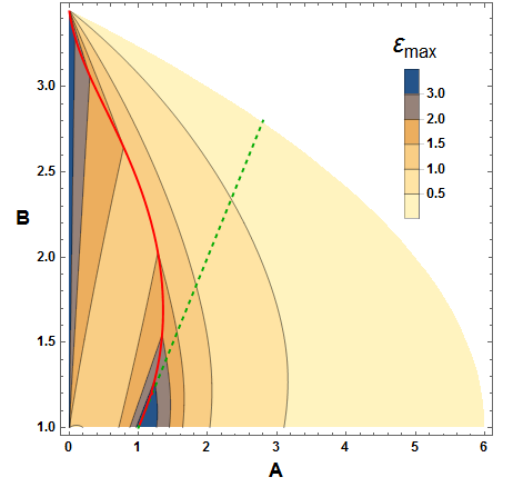
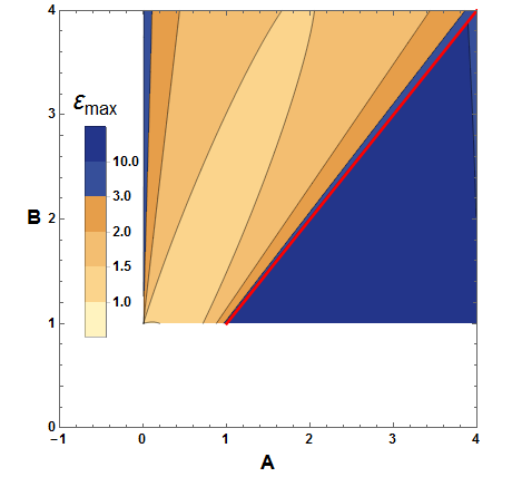
The discussion about the stability and consistency of this model is also mentioned in the Appendix. In summary, we find that for there are two new regions in the parameter space that allow small velocities and (i.e. a very elastic material), as can be seen in Figs. 9, 10. The first region is close to the line but with (). The other one extends for relatively close to . These two regions are conceptually on a different level from the EFT standpoint because the constraint on arises from gradient instability or superluminality in either case. The separatrix between the two regions is given by the red line in the plots. For this line is very close to the line at small . Importantly, both regions contain sizeable values for . The first conclusion, then, is that, indeed, adding a large mass-density term to the Lagrangian opens up the possibility to model non-relativistic materials with sizeable shear and bulk exponents, and .
In the new region with , the subluminality condition does not play any role (for and moderate values of ), so these are reasonable candidate EFTs to model realistic materials. In this region, the EFT again ‘predicts’ that the maximum strain and the bulk/shear exponents are related in a simple way. One can see that scales with the exponents as
| (25) |
Interestingly enough, even though this differs from Eq. (22) (valid for the benchmark model (15) at ) we still have some relation .
The second new region (for ) instead is only constrained by the subluminality condition, and so the bounds are less powerful. Specifically, for we find
| (26) |
Notice that the maximum strain scales as , where . This scaling can be understood because for large shear deformation the phonon speed grows as . Since the constraint obtained within the EFT is really only an upper limit on the strain, one obtains only a very large upper bound – a very loose bound.

As is clear from Figs. 9, 10, the two regions actually touch each other, therefore at some point one of the speeds must increase also in the region. Since in this region comes from the gradient instability of one of the two modes, i.e. by setting one of the speeds , a good notion of how non-relativistic the material is at the ‘breaking’ point is given by the other phonon speed, i.e. . At all the speeds are granted to be of order , while, by definition, on the separatrix between the two types of the new regions. However in truly non-relativistic materials one does not expect to raise to such large values. Therefore, in order to be more realistic, we can also impose that the speeds do not vary much from their values at equilibrium () to the breaking point. To this end, we introduce the ratio
| (27) |
and demand that in the region it is allowed to grow at most by a factor . In the limit , is only a function of and , and in the region we find, using (25),
| (28) |
This new constraint is shown in Fig. 7. This figure shows that there is indeed an overlap between the regions corresponding to large deformation ( significantly greater than 1), moderate and large exponents. The size of this region in parameter space depends on the criteria for and , but one can say that it extends to next to the line within a few percent. In this region, non-trivial relations such as (27) or (25) should hold.
As a final remark, let us emphasize the most basic property of this new region: it is close to . In other words, this corresponds to very elastic realistic materials that display a power-law stress strain curve both for shear and bulk deformations, with nearly equal bulk and shear exponents, .
V Discussion
In conclusion, let us highlight that EFT methods for solid materials allow to extract non-trivial information and bounds on their nonlinear elastic response. The list of observables that are fixed (to the leading order in the EFT) once the strain-energy function is known includes: all the -point phonon correlation functions, the phonon-phonon self-interactions and, most remarkably, how these depend on the applied stresses -- the first example of this being the acoustoelastic effect. The correlations obtained in this way are most directly relevant for materials that admit large deformations and where dissipative effects are unimportant.33 3 For recent EFT-like efforts to include dissipation in fluids and viscoelastic materials, see [46, 47, 48, 49, 50, 51, 52, 53, 54, 55, 56, 57, 58, 59].
As a specific application we have studied how the maximal strain supported by a given material is constrained by the consistency of the EFT. Focussing on the class of materials with power-law stress-strain relations at large strains, , we find several universal relations between intrinsically nonlinear response parameters, such as the maximum stress and the strain exponent.
An interesting case is represented by the conformal solids limit, realized by potentials of the form , which preserve scale invariance and imply [60] (see also [61, 62]). In this case, the bulk modulus is directly proportional to the energy density , as observed in earlier holographic models [62]. Concerning the strain exponents, scale invariance fixes and bounds . Let us emphasize, however, that the notion of a conformal solid, understood as an EFT with a Lagrangian of the above form, should be distinguished from a system whose low energy dynamics is controlled by a strongly coupled infrared fixed point. In that case, the standard EFT methods are not granted to apply. A study of the nonlinear elasticity for that case using holographic techniques is deferred to a separate work [63].
We have also shown how to extend the analysis to non-relativistic materials, with realistically small sound speeds. Our main conclusion – that the EFT method provides nontrivial relations between nonlinear response parameters – remains true also in this regime. Moreover, let us make a remark about the region close to of these non-relativistic solids. In this region, the EFT method is the most informative, so it is worth trying to compare its predictions to data. A proper analysis of the experimental data on real world elastomers is well beyond the scope of this work, but we would like to make one comment. It is known [3] that a very successful way to fit the nonlinear response of some rubbers consists of writing as a sum of a few powers of the matrix as with some constants . At large deformations, these models are dominated by the term with the highest power, call it . It is easy to see that taking does not strictly coincide with our benchmark models for any , however, it does lead to very similar response at large strains as our benchmark model with (for instance in the stress-strain relations). This is encouraging because it would suggest that the models in the region near could correspond to these rubbers. It would be interesting to see whether (27) or (25) hold for them. We leave these questions for the future.
Furthermore, it would be desirable to introduce dissipative and thermal effects within the EFT picture of condensed matter systems [64, 54]. In this regard the holographic description could provide a valuable supplementary insight [65, 62, 66, 61, 67, 62, 63, 68, 69]. We hope to return to some of these points eventually.
Acknowledgements
We thank Alex Buchel, Carlos Hoyos, Karl Landsteiner, Mikael Normann, Giuliano Panico, Napat Poovuttikul,
Kostya Trachenko and Alessio Zaccone for useful
discussions and comments about this work and the topics
considered.
MB is supported in part by the Advanced ERC grant
SM-grav, No 669288.
VCC and OP acknowledge support by the Spanish Ministry
MEC under grant FPA2014-55613-P, FPA2017-88915-P and the Severo
Ochoa excellence program of MINECO (grant SO-2012-
0234, SEV-2016- 0588), as well as by the Generalitat
de Catalunya under grant 2014-SGR-1450.
MB would like to thank Iceland University and Queen Mary University for the warm hospitality during the completion of this work and Marianna Siouti for the unconditional support.
Appendix A Fluctuations and consistency
In order to study the stability of perturbations around the strained background configuration we expand the scalar fields as . To identify the propagating degrees of freedom we perform the decomposition into longitudinal and transverse fluctuations by splitting , with satisfying:
| (29) |
This gives two dynamical scalar modes that can be defined through:
| (30) |
Constraining the spatial dependence to and redefining we obtain the following quadratic action for the fluctuations
| (31) |
where the parameters and depend on both the shear and bulk strains, i.e., they are functions of and . The explicit expressions in terms of the derivatives of the function , defined in Eq. (15), are found to be:
| (32) | ||||
| (33) | ||||
| (34) | ||||
| (35) | ||||
| (36) | ||||
| (37) |
with all the quantities evaluated on the scalar field background solution .
Let us emphasize that for a non-diagonal matrix , the transverse and longitudinal modes remain mixed both with respect to time and spatial derivatives. In order to study the stability of fluctuations we therefore first introduce the kinetic matrix as
| (38) |
The absence of ghost-like excitations then requires that the eigenvalues of the kinetic matrix, , are positive. This gives the first condition for stable propagation of the modes: .
It is straightforward to determine the true dynamical modes described by the action (31) by working at the level of the equations of motion of the mixed fields . After Fourier transforming as we can solve for the spectrum of perturbations to obtain
| (39) |
The other conditions for consistency that we are going to impose are thus:
- •
, i.e. the absence of gradient instabilities;
- •
, i.e. the absence of superluminal modes.
The exact expressions of the kinetic eigenvalues can be put in the form
| (40) |
with
| (41) | ||||
| (42) |
Similarly the sound speeds can be expressed as
| (43) |
with
| (44) | ||||
| (45) |
Let us point out that evaluating the sound speeds at and we find that the result coincides with the standard relationships obeyed by the transverse and longitudinal phonons of the equilibrium state :
| (46) |
where and are the equilibrium energy density and pressure, as in Eq. (6) and (7). The and refer to the linearized bulk and shear moduli, defined in Eq. (13) and (12).
The conditions necessary to ensure the positivity of then read:
| (47) |
The first two constraints above can be expressed as inequalities for quadratic polynomials in . For the benchmark model we find that upon setting
| (48) |
these are satisfied for any choice of , while the last condition is fulfilled automatically for arbitrary choice of .
The conditions necessary for avoiding the gradient instability are in turn
| (49) |
and are slightly harder to satisfy. It is easy to see that by setting
| (50) |
and assuming that (48) holds the condition can be satisfied for arbitrary values of . However, for these values of the equation defines an inverse parabola in the space with two real roots only when
| (51) |
Hence the condition is only satisfied for . Since we are only interested in positive values of then we conclude that the condition imposes a constraint on the maximal allowed strain applied to our system given by:
| (52) |
Analyzing the last condition in (49) analytically becomes more involved. We find however that in the parameter region
| (53) |
the maximal strain is determined by the onset of the gradient instability and is thus given by (52). Only in the region complementary to (53) is the maximal strain fixed by requiring the absence of superluminal propagation, finding
| (54) |
We present the full constraints on the parameter space obtained numerically in the main text.
Finally, let us quote our results for the simple case of linear deformations, i.e. of zero background shear strain, i.e. . We obtain the following allowed region for the exponents :
| (55) |
More specifically, the two kinetic eigenvalues in this case are equal and given by imposing the constraint . The sound speeds are in turn given by and . The absence of gradient instabilities is thus setting and . The latter constraint can be made stronger by requiring the positivity of the bulk modulus, leading to ; the positivity of the shear modulus gives again .
We can now repeat the exercise of finding the speeds and all the constraints for the nonrelativistic solid model presented in Section IV. In the limit of infinitesimal strain, the transverse and longitudinal modes, as defined in (30), decouple at the level of the quadratic action (31). Indeed, for we find that . From the positivity of the remaining quantities we arrive to the following set of conditions on the parameters of our model:
| (56) |
The propagation speeds of the canonically normalized modes are then given as
| (57) |
We thus see that with this choice of potential both propagation speeds in the infinitesimal strain limit scale with . Hence in order to go to non-relativistic speeds we just need to set . Let us also point out that the two speeds are related as . The second term in this relation comes from the linear bulk modulus, defined in Eq. (13). For the new choice of potential it equals to and thus for a negative the bulk modulus becomes negative. Henceforth we shall only consider .
The additional term in potential also enables us to expand the allowed parameter space for . In particular, by analyzing the stability conditions (49) we find that the maximal strain is only set by the requirement of the absence of gradient instability for the parameter values . Its value remains unaffected by the new term, i.e. it does not depend on , and is still given by (52), with the additional requirement (coming from ) that .
In the remaining the parameter space the maximal strain is determined by the superluminality constraint. The new term in the potential pushes the superluminality constraint further away thus expanding the allowed region for . This is shown in Fig. 9.
References
- [1] P. M. Chaikin and T. C. Lubensky, Principles of Condensed Matter Physics (Cambridge University Press, 1995).
- [2] L. D. Landau and E. M. Lifshitz, Course of Theoretical Physics, Vol. 7,Theory of Elasticity (Pergamon Press, 1970).
- [3] Y.B.Fu and R. Ogden, Nonlinear Elasticity: Theory and Applications, London Mathematical Society lecture note series No. 283 (Cambridge University Press, Cambridge, UK, 2001).
- [4] R. W. Ogden, Non-Linear Elastic Deformations (WILEY-VCH Verlag, 1985).
- [5] R. W. Ogden, G. Saccomandi, and I. Sgura, Computational Mechanics 34, 484 (2004).
- [6] H. Leutwyler, Helv. Phys. Acta 70, 275 (1997), arXiv:hep-ph/9609466 [hep-ph] .
- [7] S. Dubovsky, T. Gregoire, A. Nicolis, and R. Rattazzi, JHEP 03, 025 (2006), arXiv:hep-th/0512260 [hep-th] .
- [8] A. Nicolis, R. Penco, F. Piazza, and R. Rattazzi, JHEP 06, 155 (2015), arXiv:1501.03845 [hep-th] .
- [9] A. Nicolis, R. Penco, and R. A. Rosen, Phys. Rev. D89, 045002 (2014), arXiv:1307.0517 [hep-th] .
- [10] S. Endlich, A. Nicolis, R. Rattazzi, and J. Wang, JHEP 04, 102 (2011), arXiv:1011.6396 [hep-th] .
- [11] M. Greiter, F. Wilczek, and E. Witten, Mod. Phys. Lett. B3, 903 (1989).
- [12] A. International, Atlas of Stress-strain Curves (ASM International, 2002).
- [13] S. Tang, Acta Mechanica 4, 92 (1967).
- [14] D. S. Hughes and J. L. Kelly, Phys. Rev. 92, 1145 (1953).
- [15] M. F. Hamilton, Y. A. Il’inskii, and E. A. Zabolotskaya, The Journal of the Acoustical Society of America 105, 639 (1999), https://doi.org/10.1121/1.426255 .
- [16] R. A. Toupin and B. Bernstein, The Journal of the Acoustical Society of America 33, 216 (1961), https://doi.org/10.1121/1.1908623 .
- [17] Z. Abiza, M. Destrade, and R. Ogden, Wave Motion 49, 364 (2012).
- [18] F. D. Murnaghan, American Journal of Mathematics 59, 235 (1937).
- [19] F. Liu, P. Ming, and J. Li, Phys. Rev. B 76, 064120 (2007).
- [20] J. Yu, A. J. Freeman, and J. H. Xu, Phys. Rev. Lett. 58, 1035 (1987).
- [21] P. Böni, J. D. Axe, G. Shirane, R. J. Birgeneau, D. R. Gabbe, H. P. Jenssen, M. A. Kastner, C. J. Peters, P. J. Picone, and T. R. Thurston, Phys. Rev. B 38, 185 (1988).
- [22] R. J. Birgeneau, C. Y. Chen, D. R. Gabbe, H. P. Jenssen, M. A. Kastner, C. J. Peters, P. J. Picone, T. Thio, T. R. Thurston, H. L. Tuller, J. D. Axe, P. Böni, and G. Shirane, Phys. Rev. Lett. 59, 1329 (1987).
- [23] K. Parlinski, Z. Q. Li, and Y. Kawazoe, Phys. Rev. Lett. 78, 4063 (1997).
- [24] J. F. Scott, Rev. Mod. Phys. 46, 83 (1974).
- [25] D. M. Clatterbuck, C. R. Krenn, M. L. Cohen, and J. W. Morris, Phys. Rev. Lett. 91, 135501 (2003).
- [26] E. B. Isaacs and C. A. Marianetti, Phys. Rev. B 89, 184111 (2014).
- [27] A. Adams, N. Arkani-Hamed, S. Dubovsky, A. Nicolis, and R. Rattazzi, JHEP 10, 014 (2006), arXiv:hep-th/0602178 [hep-th] .
- [28] G. Velo and D. Zwanziger, Phys. Rev. 188, 2218 (1969).
- [29] M. Porrati and R. Rahman, Phys. Rev. D80, 025009 (2009), arXiv:0906.1432 [hep-th] .
- [30] M. Porrati and R. Rahman, Phys. Rev. D84, 045013 (2011), arXiv:1103.6027 [hep-th] .
- [31] M. Mooney, Journal of Applied Physics 11, 582 (1940), https://doi.org/10.1063/1.1712836 .
- [32] E. Arruda and M. Boyce, Journal of the Mechanics and Physics of Solids 41, 389 (1993).
- [33] R. W. Ogden, Proceedings of the Royal Society of London A: Mathematical, Physical and Engineering Sciences 326, 565 (1972).
- [34] A. N. Gent, Rubber Chemistry and Technology 69, 59 (1996), https://doi.org/10.5254/1.3538357 .
- [35] L. R. G. Treloar, Trans. Faraday Soc. 40, 59 (1944).
- [36] D. F. Jones and L. R. G. Treloar, Journal of Physics D Applied Physics 8, 1285 (1975).
- [37] M. F. Thorpe and I. Jasiuk, Proceedings of the Royal Society of London A: Mathematical, Physical and Engineering Sciences 438, 531 (1992).
- [38] M. Gaško and G. Rosenberg, Materials Engineering - Materiálové inžinierstvo (MEMI) 18, 155 (2011).
- [39] E. Pavlina and C. Vantyne, Journal of Materials Engineering and Performance, 17, 888 (2008).
- [40] P. Zhang, S. Li, and Z. Zhang, Materials Science and Engineering: A 529, 62 (2011).
- [41] C. C. Yuan and X. K. Xi, Journal of Applied Physics 109, 033515 (2011), https://doi.org/10.1063/1.3544202 .
- [42] M. J. Zhao, Y. Liu, and J. Bi, Materials Science and Technology 21, 429 (2005), https://doi.org/10.1179/174328405X29302 .
- [43] Y. C. Wang and R. S. Lakes, Journal of Composite Materials 39, 1645 (2005), https://doi.org/10.1177/0021998305051112 .
- [44] R. Lakes and K. W. Wojciechowski, Physica Status Solidi (b) 245, 545.
- [45] B. Moore, T. Jaglinski, D. S. Stone, and R. S. Lakes, Philosophical Magazine Letters 86, 651 (2006), https://doi.org/10.1080/09500830600957340 .
- [46] S. Grozdanov and J. Polonyi, Phys. Rev. D91, 105031 (2015), arXiv:1305.3670 [hep-th] .
- [47] F. M. Haehl, R. Loganayagam, and M. Rangamani, Phys. Rev. Lett. 114, 201601 (2015), arXiv:1412.1090 [hep-th] .
- [48] F. M. Haehl, R. Loganayagam, and M. Rangamani, (2017), arXiv:1701.07896 [hep-th] .
- [49] F. M. Haehl, R. Loganayagam, and M. Rangamani, (2018), arXiv:1803.11155 [hep-th] .
- [50] P. Glorioso and H. Liu, (2018), arXiv:1805.09331 [hep-th] .
- [51] M. Crossley, P. Glorioso, and H. Liu, JHEP 09, 095 (2017), arXiv:1511.03646 [hep-th] .
- [52] J. de Boer, M. P. Heller, and N. Pinzani-Fokeeva, JHEP 08, 086 (2015), arXiv:1504.07616 [hep-th] .
- [53] K. Trachenko and V. V. Brazhkin, Reports on Progress in Physics 79, 016502 (2016), arXiv:1512.06592 [cond-mat.soft] .
- [54] K. Trachenko, Phys. Rev. E 96, 062134 (2017), arXiv:1710.01390 [cond-mat.stat-mech] .
- [55] A. J. Beekman, J. Nissinen, K. Wu, and J. Zaanen, Phys. Rev. B96, 165115 (2017a), arXiv:1703.03157 [cond-mat.str-el] .
- [56] A. J. Beekman, J. Nissinen, K. Wu, K. Liu, R.-J. Slager, Z. Nussinov, V. Cvetkovic, and J. Zaanen, Phys. Rept. 683, 1 (2017b), arXiv:1603.04254 [cond-mat.str-el] .
- [57] J. Armas, J. Gath, A. Jain, and A. V. Pedersen, (2018), arXiv:1803.00991 [hep-th] .
- [58] K. Jensen, N. Pinzani-Fokeeva, and A. Yarom, (2017), arXiv:1701.07436 [hep-th] .
- [59] K. Jensen, R. Marjieh, N. Pinzani-Fokeeva, and A. Yarom, (2018), arXiv:1804.04654 [hep-th] .
- [60] A. Esposito, S. Garcia-Saenz, A. Nicolis, and R. Penco, JHEP 12, 113 (2017), arXiv:1708.09391 [hep-th] .
- [61] L. Alberte, M. Ammon, M. Baggioli, A. Jiménez, and O. Pujolàs, JHEP 01, 129 (2018), arXiv:1708.08477 [hep-th] .
- [62] M. Baggioli and A. Buchel, (2018), arXiv:1805.06756 [hep-th] .
- [63] M. Baggioli, V. Cancer Castillo, S. Renaux-Petel, O. Pujolas, and K. Yang, to appear.
- [64] S. Endlich, A. Nicolis, R. A. Porto, and J. Wang, Phys. Rev. D88, 105001 (2013), arXiv:1211.6461 [hep-th] .
- [65] M. Baggioli and O. Pujolas, Phys. Rev. Lett. 114, 251602 (2015), arXiv:1411.1003 [hep-th] .
- [66] L. Alberte, M. Baggioli, and O. Pujolas, JHEP 07, 074 (2016a), arXiv:1601.03384 [hep-th] .
- [67] T. Andrade, M. Baggioli, A. Krikun, and N. Poovuttikul, JHEP 02, 085 (2018), arXiv:1708.08306 [hep-th] .
- [68] L. Alberte, M. Baggioli, A. Khmelnitsky, and O. Pujolas, JHEP 02, 114 (2016b), arXiv:1510.09089 [hep-th] .
- [69] S. Grozdanov and N. Poovuttikul, Phys. Rev. D97, 106005 (2018), arXiv:1801.03199 [hep-th] .
*Erratum
In Appendix A , we computed the effective action for the phonon fluctuations (see equations (A2) and (A3)). We have decomposed our fluctuations into transverse and longitudinal with respect to the wave-vector , rotated along the strain deformation of the equilibrium configuration. However, beyond linear level, for large strains, our background is not isotropic because of the presence of an external strain configuration which explicitly breaks the spatial SO(2) symmetry. Therefore, our original assumption that the field perturbations can only be made to depend on one of the spatial directions, i.e. that appears unjustified and needs to be corrected. The nonlinear strain-dependent speed of propagation of the phonon fluctuations depends crucially on the angle of propagation , which was considered to be only (longitudinal modes) and (transverse modes). In this erratum, we correct our previous results and we generalize them to a generic angle of propagation introduced as . The main results remain unchanged.
The complete expression for the speeds is tedious but straightforward to compute from the quadratic action. The angle dependence disappears in the linear limit since the background becomes isotropic again.
Using the new expressions for the velocity and scanning all the angles we require that the same consistency requirements are satisfied in all directions: no ghosts, no gradient instabilities and no superluminal modes.
In Figures 8, 9 and 10 we find the maximum strain applicable . In Fig. 8 we analyze the simplest of our benchmark models, , while in Figs. 9 and 10 we work in the extended model with given in Eq. (24) (to be compared with Figures 4, 5 and 6 ). The main difference that must be pointed out is that now we do not have anymore a region with large close to . Thus there are no hyperelastic materials with small shear exponent () anymore. Instead, the hyperelastic region at is not affected by the corrections.
Notice that this last region is the one sharing important similarities with the nonlinear response of rubber materials [3], as we explain in the Discussion section. In this sense, the match with the phenomenology of hyperelastic materials is better with these new results.

The full expression for as a function of is complicated but it simplifies in a certain region of the parameter space. Indeed, in the shaded area shown in Fig. 11, the form of is determined solely from avoidance of gradient instabilities () and reduces to the simple analytical form
| (58) |

In the main text we had found that, in the limit , increases asymptotically as
| (59) |
While this is correct for the cases it is not true that this is valid for any generic value of , so our original result was not the most restrictive one. In particular, from equation (58), we observe that our previous interpretation of the above relationship (59) as a universal correlation between the maximum strain and exponents was not correct. Instead, taking into account this angle dependence, we find an interesting universal limit
| (60) |
Let us remark that the value for close to is found for an angle that obeys . For generic values of the value of leading to the most stringent condition on the maximal allowed strain has also been found analytically, however, its exact expression is too long to be given here.
In the main text, we found another region where grows asymptotically, which is in the limit where . This feature is still present, and it is given by the same expression up to a factor :
| (61) |
Finally we would like to revisit the ratio considered for the non-relativistic potential between the speed at zero strain and at the maximum shear deformation
| (62) |
which is shown in Figure 12. Comparing with the one obtained originally we see that the parameter space has decreased only slightly. Thus, we continue to have a finite region where the is large and is moderately large (the material is non-relativistic throughout the deformation). Interestingly, this includes values of the exponents of order of a few – as seen in some real-world rubber-like materials [3].
