Quantum Belinski-Khalatnikov-Lifshitz scenario

Andrzej Góźdź Email: andrzej.gozdz@umcs.lublin.pl Affiliation: Institute of Physics, Maria Curie-Skłodowska University, pl. Marii Curie-Skłodowskiej 1, 20-031 Lublin, Poland Włodzimierz Piechocki Email: wlodzimierz.piechocki@ncbj.gov.pl Affiliation: Department of Fundamental Research, National Centre for Nuclear Research, Hoża 69, 00-681 Warszawa, Poland Grzegorz Plewa Email: grzegorz.plewa@ncbj.gov.pl Affiliation: Department of Fundamental Research, National Centre for Nuclear Research, Hoża 69, 00-681 Warszawa, Poland

August 24, 2026

Abstract

We present the quantum model of the asymptotic dynamics underlying the Belinski-Khalatnikov-Lifshitz (BKL) scenario. The symmetry of the physical phase space enables making use of the affine coherent states quantization. Our results show that quantum dynamics is regular in the sense that during quantum evolution the expectation values of all considered observables are finite. The classical singularity of the BKL scenario is replaced by the quantum bounce that presents a unitary evolution of considered gravitational system. Our results suggest that quantum general relativity has a good chance to be free from singularities.

pacs

04.60.-m, 04.60.Kz, 0420.Cv

I Introduction

It is believed that the cosmological and astrophysical singularities predicted by general relativity (GR) can be resolved at the quantum level. That has been shown to be the case in the quantization of the simplest singular GR solutions like FRW-type spacetimes (commonly used in observational cosmology). However, it is an open problem in the general case. Our paper addresses the issue of possible resolution of a generic singularity problem in GR due to quantum effects.

The Belinski, Khalatnikov and Lifshitz (BKL) conjecture is thought to describe a generic solution to the Einstein equations near spacelike singularity (see, [1, 2, 3] and references therein). Later, it was extended to deal with generic timelike singularity of general relativity[4, 5, 6]. According to the BKL scenario [1, 2], in the approach to a space-like singularity neighbouring points decouple and spatial derivatives become negligible in comparison to temporal derivatives. The conjecture is based on the examination of the dynamics toward the singularity of a Bianchi spacetime, typically Bianchi IX (BIX). The BKL scenario presents the oscillatory evolution (towards the singularity) entering the phase of chaotic dynamics (see, e.g., [7, 8]), followed by approaching the spacelike manifold with diverging curvature and matter field invariants.

The most general scenario is the dynamics of the non-diagonal BIX model. However, this dynamics is difficult to exact treatment. Qualitative analytical considerations [9, 10, 11] and numerical analysis [12] strongly suggest that in the asymptotic regime near the singularity the exact dynamics can be well approximated by much simpler dynamics (presented in the next section).

The BKL scenario based on a diagonal BIX reduces to the dynamics described in terms of the three directional scale factors dependent on an evolution parameter (time). This dynamics towards the singularity has the following properties: (i) is symmetric with respect to the permutation of the scale factors, (ii) the scale factors are oscillatory functions of time, (iii) the product of the three scale factors is proportional to the volume density decreasing monotonically to zero, and (iv) the scale factors may intersect each other during the evolution of the system. The diagonal BIX is suitable to address the vacuum case and the cases with simple matter fields. More general cases, including perfect fluid with nonzero time dependent velocity, require taking non-diagonal space metric. However, the general dynamics simplifies near the singularity and can be described by three effective scale factors, which include contribution from matter field. This effective dynamics does not have the properties (i) and (iv) of the diagonal case. More details can be found in the paper [13].

Roughly speaking, the main advantage of the non-diagonal BIX scenario is that it can be used to derive the BKL conjecture in a much simpler way than when starting from the diagonal case. Namely, considering inhomogeneous perturbations of the non-diagonal BIX metric is sufficient to derive the BKL conjecture, whereas the diagonal case needs additionally considering inhomogeneous perturbation of the matter field that would correspond, e.g., to time dependent velocity of the perfect fluid [14].

The present paper concerns the quantum fate of the asymptotic dynamics of the non-diagonal BIX model. The quantum dynamics, described by the Schrödinger equation, is regular (no divergencies of physical observables) and the evolution is unitary. The classical singularity is replaced by quantum bounce due to the continuity of the probability density.

Our paper is organized as follows: In Sec. II we recall the Hamiltonian formulation of our gravitational system and identify the topology of physical phase space. Section III is devoted to the construction of the quantum formalism. It is based on using the affine coherent states ascribed to the physical phase space, and the resolution of the unity in the carrier space of the unitary representation of the affine group. The quantum dynamics is presented in Sec. IV. Finding an explicit solution to the Schrödinger equation enables addressing the singularity problem. We conclude in the last section. Appendix A presents an alternative affine coherent states. The basis of the carrier space is defined in App. B.

II Classical dynamics

For self-consistency of the present paper, we first recall some results of Ref. [15], followed by the analysis of the topology of the physical phase space.

II.1 Asymptotic regime of general Bianchi IX dynamics

The dynamical equations of the general (nondiagonal) Bianchi IX model, in the evolution towards the singularity, take the following asymptotic form [9, 10]

\frac{d^{2}\ln a}{d\tau^{2}}=b/a-a^{2},\penalty\ \penalty\ \penalty\ \frac{d^{2}\ln b}{d\tau^{2}}=a^{2}-b/a+c/b,\penalty\ \penalty\ \penalty\ \frac{d^{2}\ln c}{d\tau^{2}}=a^{2}-c/b,

(1)

where $a,b,c$ are functions of an evolution parameter $\tau$ , and are interpreted as the effective directional scale factors of considered anisotropic universe. The solution to (1) should satisfy the dynamical constraint

\frac{d\ln a}{d\tau}\;\frac{d\ln b}{d\tau}+\frac{d\ln a}{d\tau}\;\frac{d\ln c}{d\tau}+\frac{d\ln b}{d\tau}\;\frac{d\ln c}{d\tau}-a^{2}-b/a-c/b=0\,.

(2)

Eqs. (1) and (2) define a coupled highly nonlinear system of ordinary differential equations.

The derivation of this asymptotic dynamics (1)–(2) from the exact one is based, roughly speaking, on the assumption that in the evolution towards the singularity ( $\tau\rightarrow 0$ ) the following conditions are satisfied:

a\rightarrow 0,\penalty\ \penalty\ \penalty\ b/a\rightarrow 0,\penalty\ \penalty\ \penalty\ c/b\rightarrow 0\,.

(3)

We recommend Sec. 6 of Ref. [10] for the justification of taking this assumption¹¹ 1 The directional scale factors $\{a,b,c\}$ considered here and in [9], and the ones considered in [10] named $\{A,B,C\}$ , are connected by the relations: $a=A^{2},b=B^{2},c=C^{2}$ .. The numerical simulations of the exact dynamics presented in the recent paper [12] give support to the assumption (3) as well.

The dynamics (1)–(2) defines the asymptotic regime of the BKL scenario, satisfying (3), that lasts quite a long time before the system approaches the singularity, marked by the condition $a\,b\,c\rightarrow 0$ (see [9, 10] for more details).

II.2 Hamiltonian formulation with dynamical constraint

Roughly speaking, using the canonical phase space variables $\{q_{k},p_{l}\}=\delta_{kl}$ introduced in [15]:

q_{1}:=\ln a,\penalty\ \penalty\ \penalty\ q_{2}:=\ln b,\penalty\ \penalty\ \penalty\ q_{3}:=\ln c,\penalty\ \penalty\ \penalty\ \mbox{and}\penalty\ \penalty\ \penalty\ p_{1}=\dot{q}_{2}+\dot{q}_{3},\penalty\ \penalty\ \penalty\ p_{2}=\dot{q}_{1}+\dot{q}_{3},\penalty\ \penalty\ \penalty\ p_{3}=\dot{q}_{1}+\dot{q}_{2}\,,

(4)

where “dot” denotes $d/d\tau$ , turns the constraint (2) into the Hamiltonian constraint $H_{c}=0$ defined by

H_{c}:=\frac{1}{2}(p_{1}p_{2}+p_{1}p_{3}+p_{2}p_{3})-\frac{1}{4}(p_{1}^{2}+p_{2}^{2}+p_{3}^{2})-\exp(2q_{1})-\exp(q_{2}-q_{1})-\exp(q_{3}-q_{2})=0\,,

(5)

and the corresponding Hamilton’s equations read

$\displaystyle\dot{q}_{1}$	$\displaystyle=$	$\displaystyle\frac{1}{2}(-p_{1}+p_{2}+p_{3}),$	(6)
$\displaystyle\dot{q}_{2}$	$\displaystyle=$	$\displaystyle\frac{1}{2}(p_{1}-p_{2}+p_{3}),$	(7)
$\displaystyle\dot{q}_{3}$	$\displaystyle=$	$\displaystyle\frac{1}{2}(p_{1}+p_{2}-p_{3}),$	(8)
$\displaystyle\dot{p}_{1}$	$\displaystyle=$	$\displaystyle 2\exp(2q_{1})-\exp(q_{2}-q_{1}),$	(9)
$\displaystyle\dot{p}_{2}$	$\displaystyle=$	$\displaystyle\exp(q_{2}-q_{1})-\exp(q_{3}-q_{2}),$	(10)
$\displaystyle\dot{p}_{3}$	$\displaystyle=$	$\displaystyle\exp(q_{3}-q_{2}).$	(11)

The dynamical systems analysis applied to the system (5)–(11) leads to the conclusion that there exists the set of the nonhyperbolic type of critical points $S_{B}$ , corresponding to this dynamics, defined by [15]

	$\displaystyle S_{B}:$	$\displaystyle=$	$\displaystyle\{(q_{1},q_{2},q_{3},p_{1},p_{2},p_{3})\in\bar{\mathbb{R}}^{6}\penalty\ \|\penalty\ (q_{1}\rightarrow-\infty,\penalty\ q_{2}-q_{1}\rightarrow-\infty,\penalty\ q_{3}-q_{2}\rightarrow-\infty)$		(12)
			$\displaystyle\wedge(p_{1}=0=p_{2}=p_{3}\},$		(12)

where $\bar{\mathbb{R}}:=\mathbb{R}\cup\{-\infty,+\infty\}$ .

Eqs. (12) and (3) imply that the space of singular points includes the critical points surface $S_{B}$ . It is so because $(q_{1}\rightarrow-\infty,\penalty\ q_{2}-q_{1}\rightarrow-\infty,\penalty\ q_{3}-q_{2}\rightarrow-\infty)$ implies (3) (which means $a\,b\,c\rightarrow 0$ ) for any $(p_{1},p_{2},p_{3})\in\bar{\mathbb{R}}^{3}$ .

II.3 Hamiltonian formulation devoid of dynamical constraint

There exists the reduced phase space formalism corresponding to the dynamics (5)–(11) presented in [15]. The two form $\Omega$ defining the Hamiltonian formulation, devoid of the dynamical constraint (5), is given by

\Omega=dq_{1}\wedge dp_{1}+dq_{2}\wedge dp_{2}+dt\wedge dH,

(13)

where $t:=p_{3}$ . The Hamiltonian $H$ is defined to be $H=-q_{3}$ , where $q_{3}$ is determined from the dynamical constraint (5). The variables $\{q_{1},q_{2},p_{1},p_{2}\}$ parameterise the physical phase space, $H=H(t,q_{1},q_{2},p_{1},p_{2})$ is the Hamiltonian generating the dynamics, and $t$ is an evolution parameter corresponding to the specific choice of $H$ . The Hamiltonian reads²² 2 In what follows, the choice of $H$ differs from the one presented in [15] by a factor minus one to fit properly the third term of the r.h.s. of (13).

H(t,q_{1},q_{2},p_{1},p_{2})=-q_{2}-\ln\left[-e^{2q_{1}}-e^{q_{2}-q_{1}}-\frac{1}{4}(p_{1}^{2}+p_{2}^{2}+t^{2})+\frac{1}{2}(p_{1}p_{2}+p_{1}t+p_{2}t)\right],

(14)

and Hamilton’s equations are

$\displaystyle\frac{dq_{1}}{dt}$	$\displaystyle=$	$\displaystyle\frac{\partial H}{\partial p_{1}}=\frac{p_{1}-p_{2}-t}{2F},$	(15)
$\displaystyle\frac{dq_{2}}{dt}$	$\displaystyle=$	$\displaystyle\frac{\partial H}{\partial p_{2}}=\frac{-p_{1}+p_{2}-t}{2F},$	(16)
$\displaystyle\frac{dp_{1}}{dt}$	$\displaystyle=$	$\displaystyle-\frac{\partial H}{\partial q_{1}}=\frac{-2e^{2q_{1}}+e^{q_{2}-q_{1}}}{F},$	(17)
$\displaystyle\frac{dp_{2}}{dt}$	$\displaystyle=$	$\displaystyle-\frac{\partial H}{\partial q_{2}}=1-\frac{e^{q_{2}-q_{1}}}{F},$	(18)

where

F(t,q_{1},q_{2},p_{1},p_{2}):=-e^{2q_{1}}-e^{q_{2}-q_{1}}-\frac{1}{4}(p_{1}^{2}+p_{2}^{2}+t^{2})+\frac{1}{2}(p_{1}p_{2}+p_{1}t+p_{2}t)>0.

(19)

In what follows, we do not use explicitly the relationship between the evolution parameter $\tau$ and $t$ , but it does exist. Namely, since $t=p_{3}$ , solving the dynamics (5)–(11) would give $p_{3}=p_{3}(\tau)$ . Moreover, making use of Eq. (11) we can get the essential information on the time variable: (i) $\dot{p}_{3}>0$ so that $t$ is an increasing function of $\tau$ , and (ii) integrating (11) gives $p_{3}=\int_{\tau_{1}}^{\tau_{2}}d\tau\,\exp(q_{3}-q_{2})>0$ as the integrand is positive definite.

The reduced system (15)–(18) has been obtained in the procedure of mapping the system with the Hamiltonian constraint, defined by (5)–(11), into the Hamiltonian system devoid of the constraint. In the former, the Hamiltonian $H_{c}$ is a dynamical constraint, in the latter the Hamiltonian $H$ in a generator of dynamics without the constraint. As it is known, this procedure is a sort of “one-to-many” mapping (for more details, see e.g. [16, 17] and references therein). Roughly speaking, it consists in resolving the dynamical constraint with respect to one phase space variable that is chosen to be a Hamiltonian. This procedure leads to the choice of an evolution parameter (time) as well so that the Hamiltonian and time emerge in a single step. In general, this is a highly non-unique procedure if there are no hints to this process. Here the choice of the reduction was motivated by the two circumstances: (i) the resolution of the constraint only with respect to one variable $q_{3}$ is unique, and (ii) the resulting reduced phase space is isomorphic to the Cartesian product of two affine groups. The latter has unitary irreducible representation enabling the affine coherent states quantization of the underlying gravitational system (presented in the next section).

II.4 Numerical simulations of dynamics

In what follows we present the numerical solutions of Eqs. (15)–(18) near the singularity, which corresponds to the case: $q_{1}\rightarrow-\infty$ , $q_{2}-q_{1}\rightarrow-\infty$ , $F\rightarrow 0^{+}$ . Accordingly, we choose the initial conditions in the form:

	$\displaystyle q_{1}(t_{0})=-\Lambda,\quad p_{1}(t_{0})=\frac{1}{2}\left(t_{0}+\sqrt{t_{0}^{2}-2e^{-\Lambda}(4+\delta)}\right),$
	$\displaystyle\quad q_{2}(t_{0})=-2\Lambda,\quad p_{2}(t_{0})=\frac{1}{2}\left(t_{0}-\sqrt{t_{0}^{2}-2e^{-\Lambda}(4+\delta)}\right),$		(20)

where $t_{0}$ is the initial “time”, whereas $\Lambda$ and $\delta$ denote two additional parameters. Inserting (20) into (19) one gets

F(t_{0},q_{1}(t_{0}),q_{2}(t_{0}),p_{1}(t_{0}),p_{2}(t_{0}))=\left(1+\frac{\delta}{2}\right)e^{-\Lambda}-e^{-2\Lambda}=:\tilde{F}_{0}.

(21)

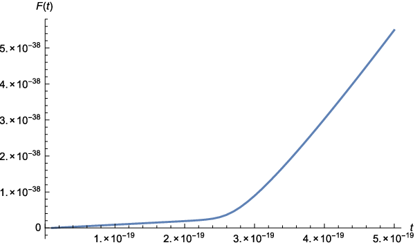
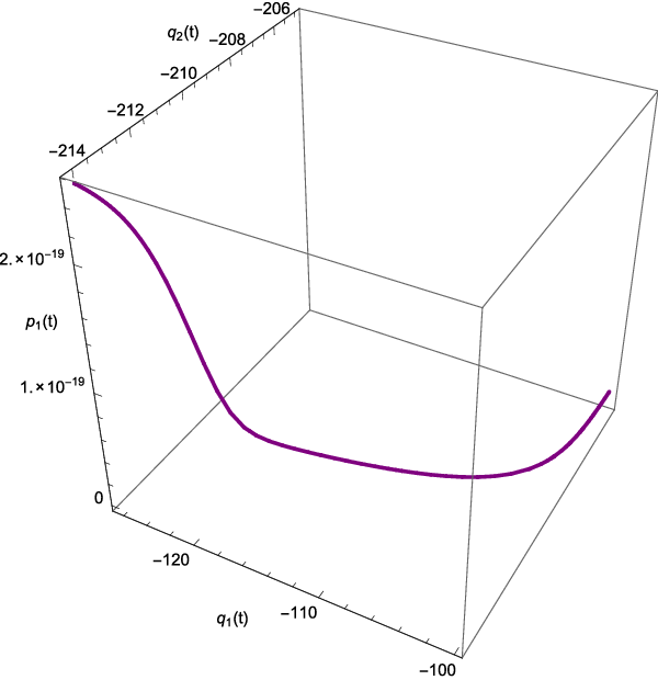
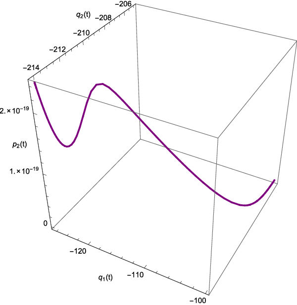
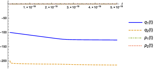
Thus, taking the limit $\Lambda\rightarrow\infty$ , while keeping $\delta$ and $t_{0}$ to be fixed, one gets $\tilde{F}_{0}\rightarrow 0^{+}$ , $q_{1}\rightarrow-\infty$ , $q_{2}-q_{1}\rightarrow-\infty$ . Therefore, (20) can be regarded as an example that ensures that we are close to the singularity. In particular, taking $\Lambda\gg 1$ and choosing $\delta>0$ to be small (but not necessarily $\delta\ll 1$ ), for a fixed $t_{0}$ , we get the vicinity of the singularity. In the next step we solve the system (15)–(18) with the boundary conditions (20). To be more specific, starting with the point in the phase space defined by (20), we can solve (15)–(18) forward or backward in time. Below, we consider the first possibility assuming $t\geq t_{0}$ . An example solution is presented in Fig 1.

The evolution with $t_{0}>t\rightarrow 0$ , becomes quickly meaningless because numerical errors grow so much that the results cannot be trusted. This is due to rapidly increasing curvature of the underlying spacetime and increasing nonlinearity effects near the surface of the nonhyperbolic critical points (12). These lead to faster and faster changes of the phase space variables parameterizing the dynamics, and finally to breaking off our numerics. We have tested that our choice $t_{0}=10^{-20}$ enables performing reliable numerical simulations for $t\geq t_{0}$ .

The solution visible in Fig 1 presents a wiggled curve in the physical phase space. This classical dynamics cannot be further extended towards the singularity (for $t<t_{0}$ ) due to the physical and mathematical reasons (and implied numerical difficulties).

II.5 Topology of phase space

Equations (15)–(18) define a coupled system of nonlinear ordinary differential equations. The solution defines the phase space of our gravitational system.

Applying the simple algebraic identity $(\alpha+\beta+\gamma)^{2}=\alpha^{2}+\beta^{2}+\gamma^{2}+2\alpha\beta+2\beta\gamma+2\alpha\gamma$ to Eq. (19) gives:

$\displaystyle F(t,q_{1},q_{2},p_{1},p_{2})$	$\displaystyle=-e^{2q_{1}}-e^{q_{2}-q_{1}}-\frac{1}{4}(p_{1}-p_{2}+t)^{2}+p_{1}t,$	(22)
$\displaystyle F(t,q_{1},q_{2},p_{1},p_{2})$	$\displaystyle=-e^{2q_{1}}-e^{q_{2}-q_{1}}-\frac{1}{4}(-p_{1}+p_{2}+t)^{2}+p_{2}t,$	(23)
$\displaystyle F(t,q_{1},q_{2},p_{1},p_{2})$	$\displaystyle=-e^{2q_{1}}-e^{q_{2}-q_{1}}-\frac{1}{4}(p_{1}+p_{2}-t)^{2}+p_{1}p_{2}.$	(24)

Combining (19) and (22) we get

p_{1}>\frac{1}{t}\left[e^{2q_{1}}+e^{q_{2}-q_{1}}+\frac{1}{4}(p_{1}-p_{2}+t)^{2}\right],

(25)

whereas (19) and (23) give

p_{2}>\frac{1}{t}\left[e^{2q_{1}}+e^{q_{2}-q_{1}}+\frac{1}{4}(-p_{1}+p_{2}+t)^{2}\right].

(26)

Making use of (19) and (24) leads to

p_{1}p_{2}>e^{2q_{1}}+e^{q_{2}-q_{1}}+\frac{1}{4}(p_{1}+p_{2}-t)^{2}.

(27)

It is clear that the signs of both r.h.s. of Eq. (25) and Eq. (26) depend only on the sign of $t$ . Since $t>0$ , we get $p_{1}>0$ and $p_{2}>0$ .

To examine the issue of well definiteness of the logarithmic function in (14), we rewrite Eq. (14) in terms of $(q_{k},p_{k})$ variables³³ 3 We stay with $p_{3}=t$ as we wish to discuss the possible sign of the time variable. as follows

q_{3}-q_{2}=\ln\left[-e^{2q_{1}}-e^{q_{2}-q_{1}}-\frac{1}{4}(p_{1}^{2}+p_{2}^{2}+t^{2})+\frac{1}{2}(p_{1}p_{2}+p_{1}t+p_{2}t)\right]\,.

(28)

At the critical surface $S_{B}$ , defined by (12), we have $q_{3}-q_{2}\rightarrow-\infty$ so the r.h.s. of (28) should have this property as well. It means that $F(t,q_{1},q_{2},p_{1},p_{2})\rightarrow 0^{+}$ on approaching $S_{B}$ so the problem of well definiteness reduces to solving the equation $t^{2}-2(p_{1}+p_{2})t+(p_{1}-p_{2})^{2}<0$ with respect to the time variable. The solution reads $(\sqrt{p_{1}}-\sqrt{p_{2}})^{2}<t<(\sqrt{p_{1}}+\sqrt{p_{2}})^{2}$ , which means that as $p_{1}\rightarrow 0$ and $p_{2}\rightarrow 0$ , we have $t\rightarrow 0^{+}$ . Therefore, our gravitational system evolves away from the singularity at $t=0$ .

The range of the variables $q_{1}$ and $q_{2}$ results from the physical interpretation ascribed to them [15]. Since $0<a<+\infty$ and $0<b<+\infty$ , we have $(q_{1},q_{2})\in\mathbb{R}^{2}$ . Thus, the physical phase space $\Pi$ consists of the two half planes:

\Pi=\Pi_{1}\times\Pi_{2}:=\{(q_{1},p_{1})\in\mathbb{R}\times\mathbb{R}_{+}\}\times\{(q_{2},p_{2})\in\mathbb{R}\times\mathbb{R}_{+}\}\;,

(29)

where $\mathbb{R}_{+}:=\{p\in\mathbb{R}\penalty\ |\penalty\ p>0\}$ . Each $\Pi_{k}\penalty\ (k=1,2)$ can be identified with the manifold of the affine group $\mathrm{Aff}(\mathbb{R})$ acting on $\mathbb{R}$ , which is sometimes denoted as “ $px+q$ ”

x^{\prime}=(q,p)\cdot x=px+q,\mbox{ where }p>0\mbox{ and }q\in\mathbb{R}\,.

This opens the possibility for quantization by affine coherent states.

It is important to notice that only the subspace

\tilde{\Pi}=\{(q_{1},p_{1},q_{2},p_{2})\colon F(t,q_{1},p_{1},q_{2},p_{2})>0\}\subset\Pi,

(30)

where $\Pi$ defined by (29), is available to the dynamics. It is due to the logarithmic function in the expression (14) defining the Hamiltonian. To make this restriction explicit, we rewrite the Hamiltonian (14) in the form

\displaystyle H(t,q_{1},q_{2},p_{1},p_{2})=\begin{cases}-q_{2}-\ln F(t,q_{1},q_{2},p_{1},p_{2}),\penalty\ \penalty\ \text{for}\penalty\ \penalty\ F(t,q_{1},q_{2},p_{1},p_{2})>0\\ 0,\penalty\ \penalty\ \penalty\ \text{for}\penalty\ \penalty\ \penalty\ F(t,q_{1},q_{2},p_{1},p_{2})<0\,\end{cases}

(31)

with $\lim_{F\rightarrow 0^{-}}H=0\penalty\ \penalty\ \text{and}\penalty\ \penalty\ \lim_{F\rightarrow 0^{+}}H=+\infty$ .

III Quantization

Suppose we have reduced phase space Hamiltonian formulation of classical dynamics of a gravitational system. It means dynamical constraints have been resolved and the Hamiltonian is a generator of the dynamics. By quantization we mean (roughly speaking) a mapping of such Hamiltonian formulation into a quantum system described in terms of quantum observables (including Hamiltonian) represented by an algebra of operators acting in a Hilbert space. The construction of the Hilbert space may make use some mathematical properties of phase space like, e.g., symplectic structure, geometry or topology. The quantum Hamiltonian is used to define the Schrödinger equation. In what follows we make specific the above procedure by using the affine coherent states approach.

III.1 Affine coherent states

The Hilbert space $\mathcal{H}$ of the entire system consists of the Hilbert spaces ${\mathcal{H}}_{1}$ and ${\mathcal{H}}_{2}$ corresponding to the phase spaces $\Pi_{1}$ and $\Pi_{2}$ , respectively. In the sequel the construction of $\mathcal{H}_{1}$ is followed by merging of $\mathcal{H}_{1}$ and $\mathcal{H}_{2}$ .

As both half-planes $\Pi_{1}$ and $\Pi_{2}$ have the same mathematical structure, the corresponding Hilbert spaces $\mathcal{H}_{1}$ and $\mathcal{H}_{2}$ are identical so we first consider only one of them. In what follows we present the formalism for $\Pi_{1}$ and $\mathcal{H}_{1}$ to be extended later to the entire system.

III.1.1 Affine coherent states for half-plane

The phase space $\Pi_{1}$ may be identified with the affine group $\mathrm{G}_{1}\equiv\mathrm{Aff}(\mathbb{R})$ by defining the multiplication law as follows

(q^{\prime},p^{\prime})\cdot(q,p)=(p^{\prime}q+q^{\prime},p^{\prime}p),

(32)

with the unity $(0,1)$ and the inverse

(q^{\prime},p^{\prime})^{-1}=(-\frac{q^{\prime}}{p^{\prime}},\frac{1}{p^{\prime}}).

(33)

The affine group has two, nontrivial, inequivalent irreducible unitary representations [18, 19, 20]. Both are realized in the Hilbert space $\mathcal{H}_{1}=L^{2}(\mathbb{R}_{+},d\nu(x))$ , where $d\nu(x)=dx/x$ is the invariant measure⁴⁴ 4 The general notion of invariant measure $dm(x)$ on the set $X$ in respect to the transformation $h:X\to X$ can be approximately defined as follows: for every function $f\colon X\to\mathbb{C}$ the integral defined by this measure fulfils the invariance condition: $\int_{X}dm(x)f(h(x))=\int_{X}dm(x)f(x)\,.$ This property is often written as: $dm(h(x))=dm(x)$ . on the multiplicative group $(\mathbb{R}_{+},\cdot)$ . In what follows we choose one of it defined by the following action:

U(q,p)\psi(x)=e^{iqx}\psi(px)\,,

(34)

where⁵⁵ 5 We use Dirac’s notation whenever we wish to deal with abstract vector, instead of functional representation of the vector. $|\psi\rangle\in L^{2}(\mathbb{R}_{+},d\nu(x))$ . Eq. (34) defines the representation as we have

U(q^{\prime},p^{\prime})[U(q,p,)\psi(x)]=U(q^{\prime},p^{\prime})[e^{iqx}\psi(px)]=e^{i(p^{\prime}q+q^{\prime})x}\psi(p^{\prime}px)\,,

and on the other hand

[U(q^{\prime},p^{\prime})U(q,p,)]\psi(x)=U(p^{\prime}q+q^{\prime},p^{\prime}p)\psi(x)=e^{i(p^{\prime}q+q^{\prime})x}\psi(p^{\prime}px)\,.

This action is unitary in respect to the scalar product in $L^{2}(\mathbb{R}_{+},d\nu(x))$ :

	$\displaystyle\int_{0}^{\infty}d\nu(x)[U(q,p)f_{2}(x)]^{\star}[U(q,p)f_{1}(x)]=\int_{0}^{\infty}d\nu(x)[e^{iqx}f_{2}(px)]^{\star}[e^{iqx}f_{1}(px)]$
	$\displaystyle=\int_{0}^{\infty}d\nu(x)f_{2}(px)^{\star}f_{1}(px)=\int_{0}^{\infty}d\nu(x)f_{2}(x)^{\star}f_{1}(x)\,.$		(35)

The last equality results from the invariance of the measure $d\nu(px)=d\nu(x)$ .

The affine group is not the unimodular group. The left and right invariant measures are given by

d\mu_{L}(q,p)=dq\,\frac{dp}{p^{2}}\quad\mbox{ and }\quad d\mu_{R}(q,p)=dq\,\frac{dp}{p},

(36)

respectively.

The left and right shifts of any group $\mathrm{G}$ are defined differently by different authors. Here we adopt the definition from [22]:

\mathcal{L}^{L}_{h}f(g)=f(h^{-1}g)\quad\mbox{and}\quad\mathcal{L}^{R}_{h}f(g)=f(gh^{-1})

(37)

for a function $f:\mathrm{G}\to\mathbb{C}$ and all $g\in\mathrm{G}$ .

For simplicity of notation, let us define integrals over the affine group $\mathrm{G}_{1}=\mathrm{Aff}(\mathbb{R})$ as:

\int_{\mathrm{G}_{1}}d\mu_{L}(q,p)=\frac{1}{2\pi}\int_{-\infty}^{+\infty}dq\int_{0}^{\infty}\frac{dp}{p^{2}}\quad\mbox{and}\quad\int_{\mathrm{G}_{1}}d\mu_{R}(q,p)=\frac{1}{2\pi}\int_{-\infty}^{+\infty}dq\int_{0}^{\infty}\frac{dp}{p}\,.

(38)

In many formulae it is useful to use shorter notation for points in the phase space $\xi\equiv(q,p)$ and identify them with elements of the affine group. In this case the product (32) is denoted as $\xi^{\prime}\cdot\xi$ . Depending on needs we will use both notations.

Fixing the normalized vector $|\Phi\rangle\in L^{2}(\mathbb{R}_{+},d\nu(x))$ , called the fiducial vector, one can define a continuous family of affine coherent states $|q,p\rangle\in L^{2}(\mathbb{R}_{+},d\nu(x))$ as follows

|q,p\rangle=U(q,p)|\Phi\rangle.

(39)

As we have two invariant measures, one can define two operators which potentially can lead to the unity in the space $L^{2}(\mathbb{R}_{+},d\nu(x))$ :

B_{L}=\int_{\mathrm{G}_{1}}d\mu_{L}(q,p)|q,p\rangle\langle q,p|\quad\mbox{and}\quad B_{R}=\int_{\mathrm{G}_{1}}d\mu_{R}(q,p)|q,p\rangle\langle q,p|\,.

(40)

Let us check which one is invariant under the action $U(q,p)$ of the affine group:

U(q^{\prime},p^{\prime})B_{L}U(q,p)^{\dagger}=\int_{\mathrm{G}_{1}}d\mu_{L}(q,p)|p^{\prime}q+q^{\prime},p^{\prime}p\rangle\langle p^{\prime}q+q^{\prime},p^{\prime}p|\,.

(41)

One needs to replace the variables under integral:

	$\displaystyle\tilde{q}=p^{\prime}q+q^{\prime}\quad\mbox{and}\quad\tilde{p}=p^{\prime}p$		(42)
	$\displaystyle q=\frac{1}{p^{\prime}}(\tilde{q}-q^{\prime})\quad\mbox{and}\quad p=\frac{\tilde{p}}{p^{\prime}}.$		(43)

Calculating the Jacobian $\frac{\partial(q,p)}{\partial(\tilde{q},\tilde{p})}=\frac{1}{(p^{\prime})^{2}}$ one gets

d\mu_{L}(q,p)=\frac{1}{p^{2}}\frac{1}{(p^{\prime})^{2}}d\tilde{q}d\tilde{p}=\frac{1}{\tilde{p}^{2}}d\tilde{q}d\tilde{p}=d\mu_{L}(\tilde{q},\tilde{p})\,.

(44)

The last result proves that

U(q^{\prime},p^{\prime})B_{L}U(q,p)^{\dagger}=\int_{\mathrm{G}_{1}}d\mu_{L}(\tilde{q},\tilde{p})|\tilde{q},\tilde{p}\rangle\langle\tilde{q},\tilde{p}|=B_{L}\,.

(45)

This also means that $B_{R}$ is not invariant under the action $U(q,p)$ .

The irreducibility of the representation, used to define the coherent states (39), enables making use of Schur’s lemma [23], which leads to the resolution of the unity in $L^{2}(\mathbb{R}_{+},d\nu(x))$ :

\int_{\mathrm{G}_{1}}d\mu_{L}(q,p)|q,p\rangle\langle q,p|=A_{\Phi}\;\mathbb{I}\;,

(46)

where the constant $A_{\Phi}$ can be determined by using any arbitrary, normalized vector $|f\rangle\in L^{2}(\mathbb{R}_{+},d\nu(x))$ :

A_{\Phi}=\int_{\mathrm{G}_{1}}d\mu_{L}(q,p)\,\langle f|q,p\rangle\langle q,p|f\rangle\,.

(47)

This formula can be calculated by making use of the invariance of the measure:

	$\displaystyle A_{\Phi}=\int_{\mathrm{G}_{1}}d\mu_{L}(q,p)$
	$\displaystyle\times\int_{0}^{\infty}d\nu(x^{\prime})\int_{0}^{\infty}d\nu(x)(f(x^{\prime})^{\star}e^{iqx^{\prime}}\Phi(px^{\prime}))(e^{-iqx}\Phi(px)^{\star}f(x))$
	$\displaystyle=\int_{0}^{\infty}\frac{dx^{\prime}}{x^{\prime}}\int_{0}^{\infty}\frac{dx}{x}\int_{0}^{\infty}\frac{dp}{p^{2}}\left[\frac{1}{2\pi}\int_{-\infty}^{+\infty}dqe^{iq(x^{\prime}-x)}\right]f(x^{\prime})^{\star}f(x)\Phi(px^{\prime})\Phi(px)^{\star}$
	$\displaystyle=\int_{0}^{\infty}\frac{dx}{x^{2}}\|f(x)\|^{2}\int_{0}^{\infty}\frac{dp}{p^{2}}\|\Phi(px)\|^{2}$
	$\displaystyle=\left(\int_{0}^{\infty}\frac{dx}{x}\|f(x)\|^{2}\right)\left(\int_{0}^{\infty}\frac{dp}{p^{2}}\|\Phi(p)\|^{2}\right)=\int_{0}^{\infty}\frac{dp}{p^{2}}\|\Phi(p)\|^{2}$		(48)

because $\langle f|f\rangle=1$ . Thus, the normalization constant is dependent on the fiducial vector. Appendix A presents alternative affine coherent states.

III.1.2 Structure of the fiducial vector

The problem which influences the structure of quantum state space is a possible degeneration of the space due to specific structure of the fiducial vector. In the case of quantum states the vectors which differ by a phase factor represent the same quantum state. Thus, let us consider the states satisfying the above condition for physically equivalent state vectors [24]:

U(\tilde{q},\tilde{p})\Phi(x)=e^{i\beta(\tilde{q},\tilde{p})}\Phi(x),\penalty\ \penalty\ \mbox{ where }\penalty\ \penalty\ \penalty\ \penalty\ \beta(\tilde{q},\tilde{p})\in\mathbb{R}.

(49)

The phase space points $\tilde{\xi}=(\tilde{q},\tilde{p})$ treated as elements of the affine group $\mathrm{Aff}(\mathbb{R})$ forms its subgroup $\mathrm{G}_{\Phi}$ . The left-hand side of Eq. (49) can be rewritten as:

e^{i\tilde{q}x}\Phi(\tilde{p}x)=e^{i\beta(\tilde{q},\tilde{p})}\Phi(x)\,.

(50)

If the generalized stationary group $\mathrm{G}_{\Phi}$ of the fiducial vector $\Phi$ is a nontrivial group, then the phase space points $(q^{\prime},p^{\prime})$ and $(\tilde{q},\tilde{p})\cdot(q^{\prime},p^{\prime})=(\tilde{p}q^{\prime},\tilde{p}p^{\prime})$ are represented by the same state vector $U(q^{\prime},p^{\prime})\Phi(x)$ , for all transformations $(\tilde{q},\tilde{p})\in\mathrm{G}_{\Phi}$ . This is due to the equality

U(q^{\prime},p^{\prime})\Phi(x)=U((\tilde{q},\tilde{p})\cdot(q^{\prime},p^{\prime}))\Phi(x).

(51)

In this case, to have a unique relation between phase space and the quantum states, the phase space has to be restricted to the quotient structure $\mathrm{Aff}(\mathbb{R})/\mathrm{G}_{\Phi}$ . From the physical point of view, in most cases, this is an undesired property.

How to construct the fiducial vector to have $\mathrm{G}_{\Phi}=\{e_{G}\}$ , where $e_{G}$ is the unit element in this group? It is seen that Eq. (50) cannot be fulfilled for $\tilde{q}\neq 0$ , independently of chosen fiducial vector. This suggests that the generalized stationary group $\mathrm{G}_{\Phi}$ is parameterized only by the momenta $(0,\tilde{p})$ , i.e. it has to be a subgroup of the multiplicative group of positive real numbers, $\mathrm{G}_{\Phi}\subseteq(\mathbb{R}_{+},\cdot)$ .

On the other hand, Eq. (50) implies that $|\Phi(\tilde{p}x)|=|\Phi(x)|$ for all $(0,\tilde{p})\in\mathrm{G}_{\Phi}$ . In addition, for the fiducial vectors $\Phi(x)=|\Phi(x)|e^{i\gamma(x)}$ the phases of these complex functions are bounded by $0\leq\gamma(x)<2\pi$ . Due to Eq. (50) the phases $\gamma(x)$ and $\beta(0,\tilde{p})$ have to fulfil the following condition $\gamma(\tilde{p}x)-\gamma(x)=\beta(0,\tilde{p})$ . One of the solutions to this equation is the logarithmic function $\gamma(x)=\ln(x)$ .

In what follows, to have the unique representation of the phase space as a group manifold of the affine group, we require the generalized stationary group to be the group consisted only of the unit element. This can be achieved by the appropriate choice of the fiducial vector.

The unit operator (46) depends explicitly on the fiducial vector

\mathbb{I}[\Phi]=\frac{1}{A_{\Phi}}\int_{\mathrm{G}_{1}}d\mu_{L}(\xi)U(\xi)|\Phi\rangle\langle\Phi|U(\xi)^{\dagger}\;,

(52)

This suggests that the most natural transformation of vectors from the representation given by the fiducial vector $|\Phi\rangle$ to the representation given by another fiducial vector $|\Phi^{\prime}\rangle$ can be constructed as the product of two unit operators $\mathbb{I}[\Phi^{\prime}]\mathbb{I}[\Phi]$ .

Let us consider an arbitrary vector $|\Psi\rangle\in L^{2}(\mathbb{R}_{+},d\nu(x))$ and its representation in the space spanned with a help of the fiducial vector $|\Phi\rangle$ :

|\Psi\rangle=\mathbb{I}[\Phi]|\Psi\rangle=\frac{1}{A_{\Phi}}\int_{\mathrm{G}_{1}}d\mu_{L}(\xi)U(\xi)|\Phi\rangle\langle\Phi|U(\xi)^{\dagger}|\Psi\rangle

(53)

The same vector can be represented in terms of another fiducial vector $|\Phi^{\prime}\rangle$ :

|\Psi\rangle=\mathbb{I}{[\Phi^{\prime}]|\Psi\rangle}=\frac{1}{A_{\Phi^{\prime}}}\int_{\mathrm{G}_{0}}d\mu_{L}(\xi)U(\xi)|\Phi^{\prime}\rangle\langle\Phi^{\prime}|U(\xi)^{\dagger}|\Psi\rangle

(54)

However, one can transform the vector (53) into the vector (54) using the product of two unit operators:

	$\displaystyle\|\Psi\rangle=\mathbb{I}[\Phi^{\prime}]\mathbb{I}[\Phi]\|\Psi\rangle=\frac{1}{A_{\Phi^{\prime}}}\frac{1}{A_{\Phi}}\int_{\mathrm{G}_{1}}d\mu_{L}(q,p)\int_{\mathrm{G}_{1}}d\mu_{L}(q^{\prime},p^{\prime})U(\xi)\|\Phi^{\prime}\rangle$
	$\displaystyle\langle\Phi^{\prime}\|U(\xi^{-1}\cdot\xi^{\prime})\|\Phi\rangle\langle\Phi\|U(\xi^{\prime})^{\dagger}\|\Psi\rangle$		(55)

Thus, the choice of the fiducial vector is formally irrelevant. However, as we will see later a relation between the classical model and its quantum realization depends on this choice. The sets of affine coherent states generated from different fiducial vectors may be not unitarily equivalent, but lead in each case to acceptable affine representations of the Hilbert space [21].

III.1.3 Phase space and quantum state spaces

The quantization procedure requires understanding the relations among the classical phase space and quantum states space. We have three spaces to be considered:

•

The phase space $\Pi$ , which consists of two half-planes $\Pi_{1}$ and $\Pi_{2}$ defined by (29). It is the background for the classical dynamics⁶⁶ 6 For simplicity we consider here only one half-plane, but the results can be easily extended to $\Pi$ ..
•

The carrier spaces $\mathcal{H}_{1}:=L^{2}(\mathbb{R}_{+},d\nu(x))$ of the unitary representation $U(q,p)$ , with the scalar product defined as

$\langle\psi_{2}|\psi_{1}\rangle=\int_{0}^{\infty}\frac{dx}{x}\,\psi_{2}^{\star}(x)\psi_{1}(x)\,.$ (56)

•

The space of square integrable functions on the affine group $\mathcal{K}_{G}=L^{2}(\mathrm{Aff}(\mathbb{R}),d\mu_{L}(q,p))$ . The scalar product is defined as follows

\langle\psi_{G2}|\psi_{G1}\rangle_{G}=\frac{1}{A_{\phi}}\int_{\mathrm{Aff}}d\mu_{L}(q,p)\psi_{G2}^{\star}(q,p)\psi_{G1}(q,p)\,,

(57)

where $\psi_{G}(q,p):=\langle q,p|\psi\rangle=\langle\Phi|U(q,p)^{\dagger}|\psi\rangle$ with $|\psi\rangle\in\mathcal{H}_{1}$ . The Hilbert space $\mathcal{K}_{G}$ is defined to be the completion in the norm induced by (57) of the span of the $\psi_{G}$ functions.

We show below that the spaces $\mathcal{H}_{1}$ and $\mathcal{K}_{G}$ are unitary isomorphic. First, one needs to check that the functions $\psi_{G}\in\mathcal{K}_{G}$ are square integrable function belonging to $L^{2}(\mathrm{Aff}(\mathbb{R}),d\mu_{L}(q,p))$ . Using the decomposition of unity we get

\frac{1}{A_{\Phi}}\int_{\mathrm{G}_{1}}d\mu_{L}(q,p)|\langle q,p|\psi\rangle|^{2}<\langle\psi|\psi\rangle_{\mathcal{H}_{1}}<\infty.

(58)

The definition of the space $\mathcal{K}_{G}$ shows that for every $\psi_{1},\psi_{2}\in\mathcal{H}_{l}$ we have the corresponding functions $\psi_{G1},\psi_{G2}$ for which the scalar products are equal (unitarity of the transformation between both spaces): $\langle\psi_{2}|\psi_{1}\rangle_{\mathcal{H}_{1}}=\langle\psi_{G1}|\psi_{G2}\rangle_{\mathcal{K}_{G}}$ .

Let us now denote by $|e_{n}\rangle$ the orthonormal basis in $\mathcal{H}_{1}$ (see App. B). The corresponding functions $e_{Gn}(q,p)=\langle q,p|e_{n}\rangle$ furnish the orthonormal set:

	$\displaystyle\langle e_{Gn}\|e_{Gm}\rangle_{\mathcal{K}_{G}}=\frac{1}{A_{\Phi}}\int_{\mathrm{G}_{1}}d\mu_{L}(q,p)e_{Gn}^{\star}(q,p)e_{Gm}(q,p)$
	$\displaystyle=\frac{1}{A_{\Phi}}\int_{\mathrm{G}_{1}}d\mu_{L}(q,p)\langle e_{n}\|q,p\rangle\langle q,p\|e_{m}\rangle=\langle e_{n}\|e_{m}\rangle=\delta_{nm}\,.$		(59)

It is obvious that the vectors $|e_{Gn}\rangle$ define the orthonormal basis in the space $\mathcal{K}_{G}$ . For every vector $|\psi\rangle\in\mathcal{H}_{1}$

|\psi\rangle=\sum_{n}\langle e_{n}|\psi\rangle|e_{n}\rangle.

(60)

Closing both sides of the above equation with $\langle q,p|$ gives the unique decomposition of the vector $\psi_{G}(q,p)\equiv\langle q,p|\psi\rangle\in\mathcal{K}_{G}$ in the basis $|e_{Gn}\rangle_{G}$ :

\psi_{G}(q,p)\equiv\langle q,p|\psi\rangle=\sum_{n}\langle e_{n}|\psi\rangle\langle q,p|e_{n}\rangle=\sum_{n}\langle e_{n}|\psi\rangle|e_{Gn}\rangle_{G}.

(61)

Note that the vector $|\psi\rangle\in\mathcal{H}_{1}$ and the vector $|\psi_{G}\rangle\in\mathcal{K}_{G}$ have the same expansion coefficients in the corresponding bases. This define the unitary isomorphism between both spaces. It means that we can work either with the quantum state space represented by the space $\mathcal{H}_{1}$ or $\mathcal{K}_{G}$ .

III.1.4 Affine coherent states for the entire system

The phase space $\Pi$ of our classical system has the structure of the Cartesian product of the two phase spaces: $\Pi=\Pi_{1}\times\Pi_{2}$ . The partial phase spaces $\Pi_{l}$ , where $l=1,2$ , are identified with the corresponding affine groups which we denote by $\mathrm{G}_{l}=\mathrm{Aff}_{l}(\mathbb{R})$ . The simple product of both affine groups $\mathrm{G}_{\Pi}=(\mathrm{G}_{1}=\mathrm{Aff}_{1}(\mathbb{R}))\times(\mathrm{G}_{2}=\mathrm{Aff}_{2}(\mathbb{R}))$ can be identified with the whole phase space $\Pi$ :

(\xi_{1},\xi_{2})\to|\xi_{1},\xi_{2}\rangle=U(\xi_{1},\xi_{2})|\Phi\rangle:=U_{1}(\xi_{1})\otimes U_{2}(\xi_{2})|\Phi\rangle,

(62)

where $\xi_{l}=(q_{l},p_{l})$ , $l=1,2,$ the fiducial vector $|\Phi\rangle$ belongs to the simple product of two Hilbert spaces $(\mathcal{H}_{1}=L^{2}(\mathbb{R}_{+},d\nu(x_{1})))\times(\mathcal{H}_{2}=L^{2}(\mathbb{R}_{+},d\nu(x_{2})))=L^{2}(\mathbb{R}_{+}\times\mathbb{R}_{+},d\nu(x_{1},x_{2}))$ , and where the measure $d\nu(x_{1},x_{2})=d\nu(x_{1})d\nu(x_{2})$ . The scalar product in $\mathcal{H}=L^{2}(\mathbb{R}_{+}\times\mathbb{R}_{+},d\nu(x_{1},x_{2}))$ reads

\langle\psi_{2}|\psi_{1}\rangle=\int_{0}^{\infty}d\nu(x_{1})\int_{0}^{\infty}d\nu(x_{2})\psi_{1}(x_{1},x_{2})^{\star}\psi_{2}(x_{1},x_{2})\,.

(63)

The fiducial vector $\Phi(x_{1},x_{2})$ is constructed as a product of two fiducial vectors $\Phi(x_{1},x_{2})=\Phi_{1}(x_{1})\Phi_{2}(x_{2})$ generating the appropriate quantum partners for the phase spaces $\Pi_{1}$ and $\Pi_{2}$ . The fiducial vector of this type does not add any correlations between both partial phase spaces. A nonseparable form of $\Phi(x_{1},x_{2})$ might lead to reducible representation of $G_{\Pi}$ in which case Schur’s lemma could not be applied to get the resolution of unity in $\mathcal{H}$ .

Let us denote by $\hat{\mathbb{I}}_{12}$ the linear extension of the tensor product $\hat{\mathbb{I}}_{1}\otimes\hat{\mathbb{I}}_{2}$ , where the unit operators in $\mathcal{H}_{k}$ are expressed in terms of the appropriate coherent states

\hat{\mathbb{I}}_{k}=\frac{1}{A_{\Phi_{k}}}\int_{\mathrm{G}_{k}}d\mu_{L}(\xi_{k})U_{k}(\xi_{k})|\Phi_{k}\rangle\langle\Phi_{k}|U_{k}(\xi_{k})^{\dagger},\penalty\ \penalty\ \penalty\ \penalty\ k=1,2.

(64)

Let us consider the orthonormal basis $\{e^{(1)}_{n}(x_{1})\otimes e^{(2)}_{n}(x_{2})\}$ in the Hilbert space $\mathcal{H}$ and an arbitrary vector $\Psi(x_{1},x_{2})=\sum_{nm}a_{nm}e^{(1)}_{n}(x_{1})\otimes e^{(2)}_{m}(x_{2})$ belonging to this space (where the basis $e_{n}(x)$ is defined in App. B). Acting on this vector with the operator $\hat{\mathbb{I}}_{12}$ one gets:

\displaystyle\hat{\mathbb{I}}_{12}\Psi(x_{1},x_{2})=\sum_{nm}a_{nm}(\hat{\mathbb{I}}_{1}e^{(1)}_{n}(x_{1}))\otimes(\hat{\mathbb{I}}_{2}e^{(2)}_{m}(x_{2}))=\Psi(x_{1},x_{2}).

(65)

The operator $\hat{\mathbb{I}}_{12}$ is identical with the unit operator $\hat{\mathbb{I}}$ on the space $\mathcal{H}$ .

The explicit form of the action of the group $\mathrm{G}_{\Pi}$ on the vector $\Psi(x_{1},x_{2})$ reads:

	$\displaystyle U(q_{1},p_{1},q_{2},p_{2})\Psi(x_{1},x_{2})=\sum_{nm}a_{nm}\{U_{1}(q_{1},p_{1})e^{(1)}_{n}(x_{1})\}\otimes\{U(q_{2},p_{2})e^{(2)}_{m}(x_{2})\}$
	$\displaystyle=\sum_{nm}a_{nm}\{e^{iqx_{1}}e^{(1)}_{n}(p_{1}x_{1})\}\otimes\{e^{iqx_{2}}e^{(2)}_{m}(p_{2}x_{2})\}=e^{iq_{1}x_{1}}e^{iq_{2}x_{2}}\sum_{nm}a_{nm}e^{(1)}_{n}(p_{1}x_{1})\otimes e^{(2)}_{m}(p_{2}x_{2})$
	$\displaystyle=e^{iq_{1}x_{1}}e^{iq_{2}x_{2}}\Psi(p_{1}x_{1},p_{2}x_{2})\,.$		(66)

III.2 Quantum observables

Making use of the resolution of the identity (46), we define the quantization of a classical observable $f$ on a half-plane as follows [26]

\mathcal{F}\ni f\longrightarrow\hat{f}:=\frac{1}{A_{\Phi}}\int_{\mathrm{G}_{1}}d\mu_{L}(q,p)|q,p\rangle f(q,p)\langle q,p|\in\mathcal{A}\,,

(67)

where $\mathcal{F}$ is a vector space of real continuous functions on a phase space, and $\mathcal{A}$ is a vector space of operators (quantum observables) acting in the Hilbert space $\mathcal{H}_{1}=L^{2}(\mathbb{R}_{+},d\nu(x))$ . It is clear that (67) defines a linear mapping and the observable $\hat{f}$ is a symmetric (Hermitian) operator. Let us evaluate the norm of the operator $\hat{f}$ :

\|\hat{f}\|\leq\frac{1}{A_{\Phi}}\int_{\mathrm{G}_{1}}d\mu_{L}(q,p)|f(q,p)|\||q,p\rangle\langle q,p|\|\leq\frac{1}{A_{\Phi}}\int_{\mathrm{G}_{1}}d\mu_{L}(q,p)|f(q,p)|\,.

(68)

This implies that, if the classical function $f$ belongs to the space of integrable functions $L^{1}(\mathrm{Aff(\mathbb{R})},d\mu_{L}(q,p))$ , the operator $\hat{f}$ is bounded so it is a self-adjoint operator. Otherwise, it is defined on a dense subspace of $L^{2}(\mathbb{R}_{+},d\nu(x))$ and its possible self-adjointness becomes an open problem as symmetricity does not assure self-adjointness so that further examination is required [27]. The quantization (67) can be applied to any type of observables including non-polynomial ones, which is of primary importance for us due to the functional form of the Hamiltonian (14).

It is important to indicate that in the case the classical observable $f$ is defined only on a subspace of the full phase space, the corresponding quantum operator $\hat{f}$ obtained via (67) acts in the entire Hilbert space corresponding to the full phase space. This is the peculiarity of the coherent states quantization [28]. Roughly speaking, it results from the non-zero overlap, $\langle q,p|q^{\prime},p^{\prime}\rangle\neq 0$ , of any two coherent states of the entire Hilbert space. In particular, the classical Hamiltonian (31) is defined on the subspace $\tilde{\Pi}$ of $\Pi$ . Hovever, the corresponding quantum Hamiltonian (71) acts in the Hilbert space $L^{2}(\mathbb{R}_{+}\times\mathbb{R}_{+},d\nu(x_{1},x_{2}))$ corresponding to $\Pi$ .

It is not difficult to show that the mapping (67) is covariant in the sense that one has

U(\xi_{0})\hat{f}U^{\dagger}(\xi_{0})=\frac{1}{A_{\Phi}}\int_{\mathrm{G}_{1}}d\mu_{L}(\xi)|\xi\rangle f(\xi_{0}^{-1}\cdot\xi)\langle\xi|=\widehat{\mathcal{L}^{L}_{\xi_{0}}f}\,,

(69)

where $\mathcal{L}^{L}_{\xi_{0}}f(\xi)=f(\xi_{0}^{-1}\cdot\xi)$ is the left shift operation (37) and $\xi_{0}^{-1}\cdot\xi=(q_{0},p_{0})^{-1}\cdot(q,p)=(\frac{q-q_{0}}{p_{0}},\frac{p}{p_{0}})$ .

The mapping (67) extended to the Hilbert space $\mathcal{H}=L^{2}(\mathbb{R}_{+}\times\mathbb{R}_{+},d\nu(x_{1},x_{2}))$ of the entire system and applied to an observable $\hat{f}$ reads

\hat{f}(t)=\frac{1}{A_{\Phi_{1}}A_{\Phi_{2}}}\int_{G_{\Pi}}d\mu_{L}(\xi_{1},\xi_{2})|\xi_{1},\xi_{2}\rangle f(\xi_{1},\xi_{2})\langle\xi_{1},\xi_{2}|\,,

(70)

where $d\mu_{L}(\xi_{1},\xi_{2}):=d\mu_{L}(q_{1},p_{1})d\mu_{L}(q_{2},p_{2})$ .

IV Quantum dynamics

The mapping (70) applied to the classical Hamiltonian (14) reads

\hat{H}(t)=\frac{1}{A_{\Phi_{1}}A_{\Phi_{2}}}\int_{G_{\Pi}}d\mu_{L}(\xi_{1},\xi_{2})|\xi_{1},\xi_{2}\rangle H(t,\xi_{1},\xi_{2})\langle\xi_{1},\xi_{2}|\,,

(71)

where $t$ is an evolution parameter of the classical level.

The quantum evolution of our gravitational system is defined by the Schrödinger equation:

i\frac{\partial}{\partial s}|\Psi(s)\rangle=\hat{H}(t)|\Psi(s)\rangle\;,

(72)

where $|\Psi\rangle\in\mathcal{H}$ , and where $s$ is an evolution parameter at the quantum level.

In general, the parameters $t$ and $s$ are different. To get the consistency between the classical and quantum levels we postulate that $t=s$ , which defines the time variable at both levels. It is worth to mention that so defined time changes monotonically due to the special choice of the parameter $t$ at the classical level (see the paragraph below (19)). This way we support the interpretation that Hamiltonian is the generator of classical and corresponding quantum dynamics.

Near the gravitational singularity, the terms $\exp(2q_{1})$ and $\exp(q_{2}-q_{1})$ in the function $F$ can be neglected, see Eqs. (19) and (12), so that we have

F(t,q_{1},q_{2},p_{1},p_{2})\longrightarrow F_{0}(t,p_{1},p_{2}):=p_{1}p_{2}-\frac{1}{4}(t-p_{1}-p_{2})^{2}\,.

(73)

This form of $F$ leads to the simplified form of the Hamiltonian (31) which now reads

\displaystyle H_{0}(t,q_{2},p_{1},p_{2}):=\begin{cases}-q_{2}-\ln F_{0}(t,p_{1},p_{2}),\penalty\ \penalty\ \penalty\ \text{for}\penalty\ \penalty\ \penalty\ F_{0}(t,p_{1},p_{2})>0\\ 0,\penalty\ \penalty\ \penalty\ \text{for}\penalty\ \penalty\ F_{0}(t,p_{1},p_{2})<0\end{cases}

(74)

with $\lim_{F_{0}\rightarrow 0^{-}}H_{0}=0\penalty\ \penalty\ \text{and}\penalty\ \penalty\ \lim_{F_{0}\rightarrow 0^{+}}H_{0}=+\infty$ . In fact, the condition

F_{0}(t,p_{1},p_{2})>0

(75)

defines the available part of the physical phase space $\Pi$ for the classical dynamics, defined by (29), which corresponds to the approximation (73). Eqs. (73)–(74) define the approximation to our original Hamiltonian system, defined by Eqs. (14)–(19), to describe the dynamics in the close vicinity of the singularity.

After long, otherwise straightforward, calculations we get the Schrödinger equation (72) in the form

i\frac{\partial}{\partial t}\Psi(t,x_{1},x_{2})=\hat{H_{0}}\;\Psi(t,x_{1},x_{2}),

(76)

where

\hat{H_{0}}:=i\frac{\partial}{\partial x_{2}}-i\frac{B}{x_{2}}-K(t,x_{1},x_{2})\,,

(77)

and where $\Psi(t,x_{1},x_{2}):=\langle x_{1},x_{2}|\Psi(t)\rangle$ . The functions $B$ and $K$ are defined to be

B:=A_{\Phi_{2}}\int_{0}^{\infty}\frac{dp}{p}\,\frac{\partial{\Phi_{2}(p)}}{\partial p}\Phi_{2}^{\ast}(p)\,,

(78)

and

K(t,x_{1},x_{2}):=\frac{1}{A_{\Phi_{1}}A_{\Phi_{2}}}\;\int_{0}^{\infty}\frac{dp_{1}}{p_{1}^{2}}\int_{0}^{\infty}\frac{dp_{2}}{p_{2}^{2}}\widetilde{\ln}\big(F_{0}(t,\frac{p_{1}}{x_{1}},\frac{p_{2}}{x_{2}})\big)|\Phi_{1}(p_{1})|^{2}|\Phi_{2}(p_{2})|^{2}\,,

(79)

where

\displaystyle\widetilde{\ln}\big(F_{0}(t,\frac{p_{1}}{x_{1}},\frac{p_{2}}{x_{2}})\big):=\begin{cases}\ln\big(F_{0}(t,\frac{p_{1}}{x_{1}},\frac{p_{2}}{x_{2}})\big),\penalty\ \penalty\ \penalty\ \text{for}\penalty\ \penalty\ \penalty\ F_{0}(t,\frac{p_{1}}{x_{1}},\frac{p_{2}}{x_{2}})>0\\ 0,\penalty\ \penalty\ \penalty\ \text{for}\penalty\ \penalty\ \penalty\ F_{0}(t,\frac{p_{1}}{x_{1}},\frac{p_{2}}{x_{2}})<0\end{cases}

(80)

with $\lim_{F_{0}\rightarrow 0^{-}}\widetilde{\ln}F_{0}=0\penalty\ \penalty\ \text{and}\penalty\ \penalty\ \lim_{F_{0}\rightarrow 0^{+}}\widetilde{\ln}F_{0}=-\infty$ .

Thus, $B$ and $K$ become known after the specification of the fiducial vectors $|\Phi_{1}\rangle$ and $|\Phi_{2}\rangle$ . It results from the definition of $B$ that one has $B^{\ast}=1-B$ . The requirement of $\hat{H_{0}}$ being Hermitian, leads to the result that $\Phi_{2}(x)\in\mathbb{R}$ and $B=1/2$ . However, these results can be obtained in the case the following conditions are satisfied:

\Phi_{2}(x)=:x\tilde{\Phi}(x),\penalty\ \penalty\ \penalty\ \lim_{x\rightarrow 0^{+}}\tilde{\Phi}(x)=0,\penalty\ \penalty\ \penalty\ \lim_{x\rightarrow+\infty}\tilde{\Phi}(x)=0\,,

(81)

and

\Psi(t,x_{1},x_{2})=:\sqrt{x_{2}}\,\tilde{\Psi}(t,x_{1},x_{2}),\penalty\ \penalty\ \penalty\ \lim_{x_{2}\rightarrow 0^{+}}\tilde{\Psi}(t,x_{1},x_{2})=0,\penalty\ \penalty\ \penalty\ \lim_{x_{2}\rightarrow+\infty}\tilde{\Psi}(t,x_{1},x_{2})=0\,.

(82)

Due to the above, the equation (76) reduces to the equation

i\frac{\partial}{\partial t}\Psi(t,x_{1},x_{2})=\left(i\frac{\partial}{\partial x_{2}}-\frac{i}{2x_{2}}-K(t,x_{1},x_{2})\right)\Psi(t,x_{1},x_{2})\,.

(83)

The general solution to Eq. (83) is found to be

\Psi(t,x_{1},x_{2})=\eta(x_{1},x_{2}+t-t_{0})\,\sqrt{\frac{x_{2}}{x_{2}+t-t_{0}}}\,\exp\left(i\int_{t_{0}}^{t}K(t^{\prime},x_{1},x_{2}+t-t^{\prime})\,dt^{\prime}\right)\,,

(84)

where $t\geq t_{0}$ , and where $\eta(x_{1},x_{2}):=\Psi(t_{0},x_{1},x_{2})$ is the initial state.

In what follows, we extend the range of the time variable to include $t_{0}=0$ (we quantize the sector $t>0$ of classical dynamics).

To get insight into the meaning of the solution (84), let us consider the inner product

\langle\Psi(t)|\Psi(t)\rangle=\int_{\mathbb{R}_{+}^{2}}d\nu(x_{1},x_{2})\frac{x_{2}|\eta(x_{1},x_{2}+t)|^{2}}{x_{2}+t}=\int_{0}^{\infty}\frac{dx_{1}}{x_{1}}\int_{t}^{\infty}d{x_{2}}\frac{|\eta(x_{1},x_{2})|^{2}}{x_{2}}\,.

(85)

Thus, the norm of the solution decreases in time. To get an unitary evolution, we choose the initial state in the form

\eta(x_{1},x_{2})=0\penalty\ \penalty\ \penalty\ \penalty\ \mbox{for}\penalty\ \penalty\ \penalty\ \penalty\ x_{2}<t_{H}\,,

(86)

where $t_{H}>0$ is a parameter of our model. This condition is consistent with (82) and for $t<t_{H}$ gives

\langle\Psi(t)|\Psi(t)\rangle=\int_{0}^{\infty}\frac{dx_{1}}{x_{1}}\big(\int_{t}^{t_{H}}+\int_{t_{H}}^{\infty}\big)d{x_{2}}\frac{|\eta(x_{1},x_{2})|^{2}}{x_{2}}=\int_{0}^{\infty}\frac{dx_{1}}{x_{1}}\int_{t_{H}}^{\infty}d{x_{2}}\frac{|\eta(x_{1},x_{2})|^{2}}{x_{2}}\,,

(87)

which is time independent so that the quantum evolution is unitary.

The condition (86), which restricts $x_{2}\sim 1/p_{2}$ , see (88) and the text below it, implies that the probability of finding the system in the region with $x_{2}<t_{H}$ vanishes.

IV.1 Elementary quantum observables

The affine coherent states quantization procedure introduces the carrier space $L^{2}(\mathbb{R}_{+}^{2},d\nu(x_{1},x_{2}))$ . The elementary quantum observables, $\hat{q}_{k}$ and $\hat{p}_{k}$ , can be expressed in terms of $x_{k}\in\mathbb{R}_{+}\penalty\$ ( $k=1,2$ ). Namely, it is not difficult to find that

	$\displaystyle\hat{p_{k}}\,\psi(t,x_{1},x_{2})=\Big(\frac{1}{A_{\Phi_{k}}}\int_{0}^{\infty}\frac{dp_{k}}{p_{k}^{2}}\,p_{k}\,\|\Phi(p_{k})\|^{2}\Big)\,\frac{1}{x_{k}}\,\psi(t,x_{1},x_{2})$
	$\displaystyle=\frac{1}{A_{\Phi_{k}}}\frac{1}{x_{k}}\,\psi(t,x_{1},x_{2}),\penalty\ \penalty\ \penalty\ \penalty\ \penalty\ k=1,2\,,$		(88)

where the fiducial vector $\Phi(p_{k})$ is normalized to unity. The multiplication operators representing the generalized momenta (4) determine the physical meaning of the variables $x_{k}$ used in the description of quantum states, as proportional to the inverse of the generalized momenta. Similarly,

\hat{q_{k}}\,\psi(t,x_{1},x_{2})=(-i\frac{\partial}{\partial x_{k}}+\frac{i}{2x_{k}})\,\psi(t,x_{1},x_{2}),\penalty\ \penalty\ \penalty\ \penalty\ \penalty\ k=1,2\,,

(89)

where $\psi\in L^{2}(\mathbb{R}_{+}^{2},d\nu(x_{1},x_{2}))$ . One can show that both, $\hat{q_{k}}$ and $\hat{p_{k}}$ , are symmetric operators on the subspace of this Hilbert space, which consists of the functions satisfying

\lim_{x_{1}\to 0^{+}}\frac{1}{\sqrt{x_{1}}}\psi(x_{1},x_{2})=0=\lim_{x_{2}\to 0^{+}}\frac{1}{\sqrt{x_{2}}}\psi(x_{1},x_{2})\,.

(90)

IV.2 Singularity of dynamics

According to Sec. II, the singularity of the classical dynamics is defined by the conditions:

q_{1}\rightarrow-\infty,\penalty\ \penalty\ \penalty\ q_{2}-q_{1}\rightarrow-\infty,\penalty\ \penalty\ \penalty\ F_{0}\rightarrow 0^{+}\penalty\ \penalty\ \penalty\ \mbox{as}\penalty\ \penalty\ \penalty\ t\rightarrow 0^{+}.

(91)

It means that the singularity may only occur at $t=0$ , and one cannot see the reason for the classical dynamics of not being regular for $t>0$ .

If for the $\Psi$ satisfying the Schrödinger equation (83) we get

\lim_{t\rightarrow 0^{+}}\langle\Psi(t)|\hat{q}_{1}|\Psi(t)\rangle=-\infty,\penalty\ \penalty\ \penalty\ \lim_{t\rightarrow 0^{+}}\langle\Psi(t)|\hat{q}_{2}-\hat{q}_{1}|\Psi(t)\rangle=-\infty\,,

(92)

and in addition

\lim_{t\rightarrow 0^{+}}\langle\Psi(t)|\,\hat{F}_{0}^{(\theta)}|\Psi(t)\rangle=0\,,

(93)

our quantization fails in resolving the singularity problem of the classical dynamics⁷⁷ 7 The precise meaning of Eq. (93) will become clear in the next subsection..

The operator $\hat{F}^{(\theta)}_{0}$ , which occurs in (93), is of basic importance and is found to be

\hat{F}^{(\theta)}_{0}(t)\,\Psi(t,x_{1},x_{2})=\breve{F}^{(\theta)}_{0}(t,x_{1},x_{2})\,\Psi(t,x_{1},x_{2})\,,

(94)

where

\breve{F}^{(\theta)}_{0}(t,x_{1},x_{2}):=\frac{1}{A_{\Phi_{1}}A_{\Phi_{2}}}\;\int_{0}^{\infty}\frac{dp_{1}}{p_{1}^{2}}\int_{0}^{\infty}\frac{dp_{2}}{p_{2}^{2}}F_{0}^{(\theta)}(t,\frac{p_{1}}{x_{1}},\frac{p_{2}}{x_{2}})|\Phi_{1}(p_{1})|^{2}|\Phi_{2}(p_{2})|^{2}\,,

(95)

with

F_{0}^{(\theta)}(t,\frac{p_{1}}{x_{1}},\frac{p_{2}}{x_{2}}):=\theta\big(F_{0}(t,\frac{p_{1}}{x_{1}},\frac{p_{2}}{x_{2}})\big)\;F_{0}(t,\frac{p_{1}}{x_{1}},\frac{p_{2}}{x_{2}})\,,

(96)

where $\theta$ is the Heaviside step function defined as follows: $\theta(x)=1$ for $x>0$ and $\theta(x)=0$ for $x\leq 0$ . Therefore, $\hat{F}^{(\theta)}_{0}$ is a multiplication operator.

IV.3 Resolution of the singularity problem

In what follows, we first define an example of a regular state at $t=t_{s}>0$ . Next, we make generalization. Afterwards, we map the general regular state to the initial state at $t=0$ , by inverting the general form of the solution defined by Eqs. (84) (with $t_{0}=0$ ) and (86). Finally, we argue that the initial state is regular at $t=0$ due to the unitarity of the quantum evolution. This way we get the resolution of the initial singularity problem of the underlying classical dynamics.

IV.3.1 Regular state at fixed time

Let us define a state defined at $t=t_{s}>0$ , that is “far away” from the singularity, as follows

\displaystyle\Psi(t_{s},x_{1},x_{2})=\begin{cases}0,&\text{for }x_{2}\leq t_{H}\\ v(x_{1},x_{2})e^{i(\Lambda_{1}x_{1}+\Lambda_{2}x_{2})},&\text{for }x_{2}>t_{H},\end{cases}

(97)

where

\displaystyle v(x_{1},x_{2})=\begin{cases}0,&\text{for }x_{2}\leq t_{H}\\ \frac{1}{\sqrt{N_{v}}}\left[\frac{x_{1}^{2}}{(\beta_{1}+x_{1})^{3}}\right]\left[\frac{(x_{2}-t_{H})^{2}}{(\beta_{2}-t_{H}+x_{2})^{3}}\right],&\text{for }x_{2}>t_{H}.\end{cases}

(98)

and where $\Lambda_{1},\Lambda_{2},\beta_{1},\beta_{2}\in\mathbb{R}\penalty\$ ( $N_{v}$ denotes normalization constant).

Direct calculation gives

\langle\Psi(t_{s},x_{1},x_{2})|\hat{q}_{k}|\Psi(t_{s},x_{1},x_{2})\rangle=\Lambda_{k},\penalty\ \penalty\ \penalty\ k=1,2\,,

(99)

and

\langle\Psi(t_{s},x_{1},x_{2})|\hat{F}^{(\theta)}_{0}(t_{s})|\Psi(t_{s},x_{1},x_{2})\rangle>0\,,

(100)

as the integrand of (100) is positive definite due to (95).

One can also verify that we have

\langle\Psi(t_{s},x_{1},x_{2})|\hat{p}_{k}|\Psi(t_{s},x_{1},x_{2})\rangle=C_{p}\int_{0}^{\infty}\frac{dx_{1}}{x_{1}}\int_{t_{H}}^{\infty}dx_{2}\frac{|v(x_{1},x_{2})|^{2}}{x_{k}(x_{2}-t)}<\infty,\penalty\ \penalty\ \penalty\ k=1,2\,,

(101)

where $C_{p}$ is a constant.

Therefore, the state (97) is regular at $t_{s}$ .

IV.3.2 Initial state obtained in backward evolution

The state (97) is an example of the state that can be presented, due to (84) and (86), as follows

	$\displaystyle{\color[rgb]{0,0,0}\Psi(t_{s},x_{1},x_{2})=0,\penalty\ \penalty\ \mbox{for}\penalty\ \penalty\ x_{2}\leq t_{H}-t_{s}},\penalty\ \penalty\ \mbox{where}\penalty\ \penalty\ t_{s}<t_{H}\ ,$		(102)
	$\displaystyle\Psi(t_{s},x_{1},x_{2})=\eta(x_{1},x_{2}+t_{s})\sqrt{\frac{x_{2}}{x_{2}+t_{s}}}\times$
	$\displaystyle\times\exp\left(i\int_{0}^{t_{s}}K(t^{\prime},x_{1},x_{2}+t_{s}-t^{\prime})dt^{\prime}\right),\penalty\ \penalty\ \mbox{for}\penalty\ \penalty\ x_{2}\geq t_{H}-t_{s}\,.$		(103)

The above state can be inverted to get the initial state at $t=0$ via the backward evolution:

	$\displaystyle{\color[rgb]{0,0,0}\eta(x_{1},x_{2})=0,\penalty\ \penalty\ \mbox{ for }\penalty\ \penalty\ x_{2}\leq t_{H}}\ ,$		(104)
	$\displaystyle\eta(x_{1},x_{2})=\Psi(t_{s},x_{1},x_{2}-t_{s})\sqrt{\frac{x_{2}}{x_{2}-t_{s}}}\times$
	$\displaystyle\times\exp\left(-i\int_{0}^{t_{s}}K(t^{\prime},x_{1},x_{2}-t^{\prime})dt^{\prime}\right),\penalty\ \penalty\ \mbox{ for }\penalty\ \penalty\ x_{2}>t_{H}\ .$		(105)

Since the “forward” evolution is unitary, the “backward” evolution is unitary as well.

IV.3.3 Regularity of the initial state

It is easy to check that

\langle\eta(x_{1},x_{2})|\hat{q}_{k}|\eta(x_{1},x_{2})\rangle<\infty\,,

(106)

and

\langle\eta(x_{1},x_{2})|\hat{p}_{k}|\eta(x_{1},x_{2})\rangle=C_{p}\int_{0}^{\infty}\frac{dx_{1}}{x_{1}}\int_{t_{H}}^{\infty}dx_{2}\frac{|\Psi(t_{s},x_{1},x_{2}-t_{s})|^{2}}{x_{k}(x_{2}-t_{s})}<\infty\ ,

(107)

where $k=1,2$ and where $C_{p}$ is a constant. It is so because the integrands of (106) and (107) are positive definite functions, and due to (90).

Now, let us address the issue presented by Eq. (93). To show that this equation cannot be satisfied, we should prove that for all $t_{H}>t_{s}\neq 0$ we have

\langle\eta(x_{1},x_{2})|\hat{F}^{(\theta)}_{0}(t_{s})|\eta(x_{1},x_{2})\rangle=\int_{0}^{\infty}\frac{dx_{1}}{x_{1}}\int_{t_{H}}^{\infty}dx_{2}\frac{\breve{F}^{(\theta)}_{0}(t_{s})|\Psi(t_{s},x_{1},x_{2}-t_{s})|^{2}}{x_{2}-t_{s}}>0\,.

(108)

We exclude the case $t_{s}=0$ , because for $p_{1}=p_{2}$ , due to (96), we have $F_{0}^{(\theta)}=0$ , which means $\hat{F}_{0}^{(\theta)}(0)=\hat{0}$ . The “zero operator” cannot represent any physical observable as its action does not lead to any physical state. Namely, it maps any state $|\psi\rangle$ into the zero vector $\hat{0}|\psi\rangle$ . Such a vector cannot be normalized. Thus, it cannot be given any probabilistic interpretation.

Since the integrand defining Eq. (108) is positive definite, the equation is satisfied, which completes the proof.

Thus, the initial state is regular, i.e., does not satisfy Eqs. (92) and (93). This implies that whenever we have a regular state far away from the singularity (which is generic case), the initial quantum state at $t=0$ is regular so that the quantum evolution is well defined for any $t\geq 0$ . This is a direct consequence of the unitarity of considered quantum evolution.

IV.4 Quantum bounce

Let us examine the issue of possible time reversal invariance of our quantum model. In what follows, we examine the time reversal invariance of our Schrödinger equation and its solution.

The operator of the time reversal, $\hat{T}:\mathcal{H}\rightarrow\mathcal{H}$ , is defined to be

\hat{T}\,\psi(t,x_{1},x_{2})=\tilde{\psi}(t,x_{1},x_{2}):=\psi(-t,x_{1},x_{2})^{\ast},\penalty\ \penalty\ \penalty\ \mbox{where}\penalty\ \penalty\ \penalty\ \psi\in\mathcal{H}\,,

(109)

so its complex conjugates change the sine of the time variable in a state vector.

i\frac{\partial}{\partial t}\tilde{\Psi}(t,x_{1},x_{2})=\left(-i\frac{\partial}{\partial x_{2}}+\frac{i}{2x_{2}}-K(-t,t,x_{1},x_{2})\right)\tilde{\Psi}(t,x_{1},x_{2})\,.

(110)

The general solution to Eq. (110), for $t<0$ , is found to be

\tilde{\Psi}(t,x_{1},x_{2})=\eta(x_{1},x_{2}+|t|-|t_{0}|)\,\sqrt{\frac{x_{2}}{x_{2}+|t|-|t_{0}|}}\,\exp\left(i\int_{t_{0}}^{t}K(-t^{\prime},x_{1},x_{2}-t+t^{\prime})\,dt^{\prime}\right)\,,

(111)

where $|t|\geq|t_{0}|$ , and where $\eta(x_{1},x_{2}):=\tilde{\Psi}(t_{0},x_{1},x_{2})$ is the initial state.

The unitarity of the evolution (with $t_{0}=0$ ) leads to the condition

\eta(x_{1},x_{2})=0\penalty\ \penalty\ \penalty\ \penalty\ \mbox{for}\penalty\ \penalty\ \penalty\ \penalty\ x_{2}<|t_{H}|\,,

(112)

which corresponds to the condition (86).

For $|t|<|t_{H}|$ we get

\langle\tilde{\Psi}(t)|\tilde{\Psi}(t)\rangle=\int_{0}^{\infty}\frac{dx_{1}}{x_{1}}\int_{|t_{H}|}^{\infty}d{x_{2}}\frac{|\eta(x_{1},x_{2})|^{2}}{x_{2}}\,,

(113)

which shows that the norm is time independent.

Comparing Eqs. (83) and (110) we can see that the dynamical equation fails to be time reversal invariant because the Hamiltonian $\hat{H}_{0}$ does not have this symmetry. However, the solutions to these equations have only different phases. Thus, the probability density is continuous at $t=0$ (that marks the classical singularity) due to Eqs. (84) and (111) (with $|t_{0}|=0$ ), which we call the quantum bounce.

V Conclusions

Near the classical singularity the dynamics of the general Bianchi IX model simplifies. Due to the symmetry of the physical phase space of this model, we can apply the affine coherent states quantization method. The quantum dynamics, described by the Schrödinger equation, is devoid of singularities in the sense that the expectation values of basic operators are finite during the quantum evolution of the system. The evolution is unitary and the probability density of our system is continuous at $t=0$ , which marks the classical singularity.

We name the state defined by Eqs. (102)–(103) the rescue state. It is chosen to be regular because one expects that the quantum state far away from the singularity is a proper quantum state. The Schrödinger evolution does not lead outside the space of such states.

The choice of the fiducial state as the rescue state leads, under the action of the affine group, to another rescue state with changed parameter $t_{H}$ . Namely,

U(q,p)\mathcal{K}_{t_{H}}=\mathcal{K}_{t_{H}/p},\penalty\ \penalty\ \penalty\ \penalty\ p\in(0,+\infty),

(114)

where $\mathcal{K}_{t_{H}}$ denotes the rescue space with $t_{H}$ parameter (for simplicity we consider only one half plane). In general, the fiducial vector is known to be a free “parameter” of the coherent states quantization formalism. However, our final conclusion does not depend on the fiducial vector.

The quantum Hamiltonian, $\hat{H}_{0}(t,x_{1},x_{2})=-\hat{q}_{2}-\hat{K}(t,x_{1},x_{2})$ , is not invariant under the affine group action as we have

	$\displaystyle U_{1}(\tilde{q}_{1},\tilde{p}_{1})U_{2}(\tilde{q}_{2},\tilde{p}_{2})\hat{H}_{0}(t,x_{1},x_{2})U_{1}(\tilde{q}_{1},\tilde{p}_{1})^{-1}U_{2}(\tilde{q}_{2},\tilde{p}_{2})^{-1}$
	$\displaystyle=\hat{H}_{0}(t,\tilde{p}_{1}x_{1},\tilde{p}_{2}x_{2})=-\frac{1}{\tilde{p}_{2}}\hat{q}_{2}-\hat{K}(t,\tilde{p}_{1}x_{1},\tilde{p}_{2}x_{2})\neq\hat{H}_{0}(t,x_{1},x_{2})\,.$		(115)

Therefore, the affine coherent states quantization does not introduce the affine symmetry as the symmetry of our quantum system. However, the quantum evolution restricted to the space of all possible rescue spaces is unitary and devoid of singularities. Thus, the rescue space, which spans the subspace of our Hilbert space, is of basic importance in our quantization scheme.

The non-diagonal BIX underlies the BKL conjecture which concerns the generic singularity of general relativity. Therefore, our results suggest that quantum general relativity is free from singularities. Classical singularity is replaced by quantum bounce, which presents a unitary evolution of the quantum gravity system.

Since general relativity successfully describes almost all available gravitational data, it makes sense its quantization to get the extension to the quantum regime. The latter could be used to describe quantum gravity effects expected to occur near the beginning of the Universe and in the interior of black holes.

Our fully quantum results show that the preliminary results obtained for the diagonal BIX within the semiclassical affine coherent states approximation [29, 30] are correct. Appendix B presents the affine coherent states applied in these papers, which define another parametrization of our coherent states.

As far as we are aware, we are pioneers in addressing the issue of resolving the generic singularity problem of general relativity via quantization. Therefore, trying to confirm our preliminary results within different quantization scheme would be interesting. In particular, the choice of different time and corresponding Hamiltonian in the reduced phase space approach (see, Eq. (13)) would be valuable.

Acknowledgements.

We would like to thank Katarzyna Górska for the derivation of Eqs. (25)–(27), Vladimir Belinski and John Klauder for helpful correspondence, and Claus Kiefer for discussion.

Appendix A Alternative affine coherent states for half-plane

The phase space $\Pi_{1}$ may be identified with the affine group $\mathrm{Aff}(\mathbb{R})$ by defining the multiplication law as follows

(q^{\prime},p^{\prime})\cdot(q,p)=(\frac{q}{p^{\prime}}+q^{\prime},p^{\prime}p),

(116)

with the unity $(0,1)$ and the inverse

(q^{\prime},p^{\prime})^{-1}=(-q^{\prime}p^{\prime},\frac{1}{p^{\prime}}).

(117)

The affine group has two, nontrivial, inequivalent irreducible unitary representations [18] and [19, 20]. Both are realized in the Hilbert space $L^{2}(\mathbb{R}_{+},d\nu(x))$ , where $d\nu(x)=dx/x$ is the invariant measure on the multiplicative group $(\mathbb{R}_{+},\cdot)$ . In what follows we choose the one defined by

U(q,p)\psi(x)=e^{iqx}\psi(x/p)\,,

(118)

where $|\psi\rangle\in L^{2}(\mathbb{R}_{+},d\nu(x))$ .

For simplicity of notation, let us define integrals over the affine group $\mathrm{Aff}(\mathbb{R})$ as follows:

	$\displaystyle\int_{\mathrm{Aff}(\mathbb{R})}d\mu_{L}(q,p)=\frac{1}{2\pi}\int_{-\infty}^{+\infty}dq\int_{0}^{\infty}\frac{dp}{p^{2}}\,,$		(119)
	$\displaystyle\int_{\mathrm{Aff}(\mathbb{R})}d\mu_{R}(q,p)=\frac{1}{2\pi}\int_{-\infty}^{+\infty}dq\int_{0}^{\infty}\frac{dp}{p}\,,$		(120)
	$\displaystyle\int_{\mathrm{Aff}(\mathbb{R})}d\mu_{U}(q,p)=\frac{1}{2\pi}\int_{-\infty}^{+\infty}dq\int_{0}^{\infty}dp\,\rho(q,p)\,.$		(121)

The last one is intended to be used as invariant measure in respect with the action $U(q,p)$ .

|q,p\rangle=U(q,p)|\Phi\rangle.

(122)

As we have three measures, one can define three operators which potentially can leads to the unity in the space $L^{2}(\mathbb{R}_{+},d\nu(x))$ :

	$\displaystyle B_{L}=\int_{\mathrm{Aff}(\mathbb{R})}d\mu_{L}(q,p)\|q,p\rangle\langle q,p\|\,,$		(123)
	$\displaystyle B_{R}=\int_{\mathrm{Aff}(\mathbb{R})}d\mu_{R}(q,p)\|q,p\rangle\langle q,p\|\,,$		(124)
	$\displaystyle B_{U}=\int_{\mathrm{Aff}(\mathbb{R})}d\mu_{U}(q,p)\,\rho(q,p)\|q,p\rangle\langle q,p\|\,.$		(125)

Let us check which one is invariant under the action $U(q,p)$ of the affine group:

U(q^{\prime},p^{\prime})B_{U}U(q^{\prime},p^{\prime})^{\dagger}=\int_{-\infty}^{+\infty}dq\int_{0}^{\infty}dp\rho(q,p)|q/p^{\prime}+q^{\prime},p^{\prime}p\rangle\langle q/p^{\prime}+q^{\prime},p^{\prime}p|

(126)

One needs to replace the variables under the integral:

	$\displaystyle\tilde{q}=q/p^{\prime}+q^{\prime}\quad\mbox{and}\quad\tilde{p}=p^{\prime}p\,,$		(127)
	$\displaystyle q=p^{\prime}(\tilde{q}-q^{\prime})\quad\mbox{and}\quad p=\frac{\tilde{p}}{p^{\prime}}\,.$		(128)

Calculating the Jacobian $\frac{\partial(q,p)}{\partial(\tilde{q},\tilde{p})}=1$ one gets:

d\mu_{U}(q,p)=\rho(q,p)d\tilde{q}d\,\tilde{p}=\rho(p^{\prime}(\tilde{q}-q^{\prime}),\frac{\tilde{p}}{p^{\prime}})d\tilde{q}d\,\tilde{p}

(129)

This implies, the transformed weight should be equal to the initial one, $\rho(p^{\prime}(\tilde{q}-q^{\prime}),\frac{\tilde{p}}{p^{\prime}})=\rho(q,p)$ for every $(q^{\prime},p^{\prime})$ . The simplest solution is $\rho(q,p)=\mathrm{const}$ , so we get $d{\mu_{U}}(q,p)=dq\,dp$ .

It also implies that the operators $B_{L}$ and $B_{R}$ do not commute with the affine group. The action (118) is not compatible neither with the left invariant, nor with right invariant measures on the affine group.

The irreducibility of the representation, used to define the coherent states (122), enables making use of Schur’s lemma [23], which leads to the resolution of the unity in $L^{2}(\mathbb{R}_{+},d\nu(x))$ :

\int_{\mathrm{Aff}(\mathbb{R})}d{\mu_{U}}(q,p)|q,p\rangle\langle q,p|=A_{\Phi}\;\mathbb{I}\;,

(130)

where the constant $A_{\Phi}$ can be calculated using any arbitrary, normalized vector $|f\rangle\in L^{2}(\mathbb{R}_{+},d\nu(x))$ :

A_{\Phi}=\int_{\mathrm{Aff}(\mathbb{R})}d{\mu_{U}}(q,p)\,\langle f|q,p\rangle\langle q,p|f\rangle\,.

(131)

This formula can be calculated directly:

	$\displaystyle A_{\Phi}=\int_{\mathrm{Aff}(\mathbb{R})}d{\mu_{U}}(q,p)$
	$\displaystyle\times\int_{0}^{\infty}d\nu(x^{\prime})\int_{0}^{\infty}d\nu(x)(f(x^{\prime})^{\star}e^{iqx^{\prime}}\Phi(x^{\prime}/p))(e^{-iqx}\Phi(x/p)^{\star}f(x))$
	$\displaystyle=\int_{0}^{\infty}\frac{dx^{\prime}}{x^{\prime}}\int_{0}^{\infty}\frac{dx}{x}\int_{0}^{\infty}dp\left[\frac{1}{2\pi}\int_{-\infty}^{+\infty}dqe^{iq(x^{\prime}-x)}\right]f(x^{\prime})^{\star}f(x)\Phi(x^{\prime}/p)\Phi(x/p)^{\star}$
	$\displaystyle=\int_{0}^{\infty}\frac{dx}{x^{2}}\|f(x)\|^{2}\int_{0}^{\infty}dp\|\Phi(x/p)\|^{2}$
	$\displaystyle=\left(\int_{0}^{\infty}\frac{dx}{x}\|f(x)\|^{2}\right)\left(\int_{0}^{\infty}\frac{dp}{p^{2}}\|\Phi(p)\|^{2}\right)=\int_{0}^{\infty}\frac{dp}{p^{2}}\|\Phi(p)\|^{2}\,$		(132)

if $\langle f|f\rangle=1$ .

In the derivation of (132) we have used the equations:

\langle x|x^{\prime}\rangle=x\delta(x-x^{\prime}),\penalty\ \penalty\ \penalty\ \int_{0}^{\infty}\frac{dx}{x}\,|x\rangle\langle x|=\mathbb{I},\penalty\ \penalty\ \penalty\ \int_{0}^{\infty}\frac{dx}{x}\,\delta(x-x^{\prime})f(x)=f(x^{\prime})\,.

(133)

Appendix B Orthonormal basis of the carrier space

The basis of the Hilbert space $L^{2}(\mathbb{R}_{+},d\nu(x))$ is known to be [25]

e^{(\alpha)}_{n}(x)=\sqrt{\frac{n!}{\Gamma(n+\alpha+1)}}\,e^{-x/2}x^{(1+\alpha)/2}\,L_{n}^{(\alpha)}(x),

(134)

where $L_{n}^{(\alpha)}$ is the Laguerre function and $\alpha>-1$ . One can verify that $\int_{0}^{\infty}e^{(\alpha)}_{n}(x)e^{(\alpha)}_{m}(x)d\nu(x)=\delta_{nm}$ so that $e^{(\alpha)}_{n}(x)$ is an orthonormal basis and can be used in calculations.

References

[1] V. A. Belinskii, I. M. Khalatnikov, and E. M. Lifshitz, “Oscillatory approach to a singular point in the relativistic cosmology”, Adv. Phys. 19, 525 (1970).
[2] V. A. Belinskii, I. M. Khalatnikov, and E. M. Lifshitz, “A general solution of the Einstein equations with a time singularity”, Adv. Phys. 31, 639 (1982).
[3] V. Belinski and M. Henneaux, The Cosmological Singularity (Cambridge University Press, Cambridge, 2017).
[4] S. L. Parnovsky, “Gravitation fields near the naked singularities of the general type”, Physica A 104, 210 (1980).
[5] S. L. Parnovsky, “A general solution of gravitational equations near their singularities”, Class. Quant. Grav. 7, 571 (1990).
[6] S. L. Parnovsky and W. Piechocki, “Classical dynamics of the Bianchi IX model with timelike singularity,” Gen. Rel. Grav. 49, 87 (2017).
[7] N. J. Cornish and J. J. Levin, “The Mixmaster universe is chaotic,” Phys. Rev. Lett. 78, 998 (1997).
[8] N. J. Cornish and J. J. Levin, “The Mixmaster universe: A Chaotic Farey tale,” Phys. Rev. D 55, 7489 (1997).
[9] V. A. Belinskii, I. M. Khalatnikov, and M. P. Ryan, “The oscillatory regime near the singularity in Bianchi-type IX universes”, Preprint 469 (1971), Landau Institute for Theoretical Physics, Moscow (unpublished); published as Secs. 1 and 2 in M. P. Ryan, Ann. Phys. 70, 301 (1971).
[10] V. A. Belinski, “On the cosmological singularity”, Int. J. Mod. Phys. D 23, 1430016 (2014).
[11] R. T. Jantzen, “Spatially homogeneous dynamics: a unified picture”, arXiv:gr-qc/0102035. Originally published in the Proceedings of the International School Enrico Fermi, Course LXXXVI (1982) on Gamov Cosmology, edited by R. Ruffini and F. Melchiorri (North Holland, Amsterdam, 1987), pp. 61–147.
[12] C. Kiefer, N. Kwidzinski, and W. Piechocki, “On the dynamics of the general Bianchi IX spacetime near the singularity”, Eur. Phys. J. C 78, 691 (2018).
[13] E. Czuchry and W. Piechocki, “Asymptotic Bianchi IX model: diagonal and general cases,” arXiv:1409.2206 [gr-qc].
[14] V. Belinski, private communication.
[15] E. Czuchry and W. Piechocki, “Bianchi IX model: Reducing phase space,” Phys. Rev. D 87, 084021 (2013).
[16] P. Małkiewicz and A. Miroszewski, “Internal clock formulation of quantum mechanics,” Phys. Rev. D 96, 046003 (2017).
[17] P. Małkiewicz, “What is Dynamics in Quantum Gravity?,” Class. Quant. Grav. 34, 205001 (2017).
[18] I. M. Gel^′fand and M. A. Naïmark, “Unitary representations of the group of linear transformations of the straight line”, Dokl. Akad. Nauk. SSSR 55, 567 (1947).
[19] E. W. Aslaksen and J. R. Klauder, “Unitary Representations of the Affine Group”, J. Math. Phys. 9, 206 (1968).
[20] E. W. Aslaksen and J. R. Klauder, “Continuous Representation Theory Using Unitary Affine Group”, J. Math. Phys. 10, 2267 (1969).
[21] J. R. Klauder, private communication.
[22] J. Q. Chen, J. Ping and F. Wang, Group Representation Theory for Physicists (World Scientific, 2002).
[23] A. O. Barut and R. Ra̧czka, Theory of group representations and aplications (PWN, Warszawa, 1977).
[24] A. Perelomov, Generalized coherent states and their applications (Springer-Verlag, Berlin, 1986).
[25] J. P. Gazeau and R. Murenzi, “Covariant affine integral quantization(s),” J. Math. Phys. 57, 052102 (2016).
[26] H. Bergeron and J. P. Gazeau, “Integral quantizations with two basic examples,” Annals Phys. 344, 43 (2014).
[27] M. Reed and B. Simon, Methods of Modern Mathematical Physics (San Diego, Academic Press, 1980), Vols I and II.
[28] J. R. Klauder, Enhanced Quantization: Particles, Fields and Gravity, (World Scientific, Singapore, 2015)
[29] H. Bergeron, E. Czuchry, J. P. Gazeau, P. Małkiewicz and W. Piechocki, “Smooth quantum dynamics of the mixmaster universe,” Phys. Rev. D 92 061302 (2015).
[30] H. Bergeron, E. Czuchry, J. P. Gazeau, P. Małkiewicz and W. Piechocki, “Singularity avoidance in a quantum model of the Mixmaster universe,” Phys. Rev. D 92, 124018 (2015).