跳到论文正文
W Papers独立论文阅读器 arXiv:1807.07393 论文正文 计算阅读时间 · 0%
引用这篇论文根据当前论文元数据生成,正式投稿前建议核对。


License: arXiv.org perpetual non-exclusive license
arXiv:1807.07393v2 [math.NA] 14 May 2019

A finite difference approximation of a two dimensional time fractional advection-dispersion problem

Carlos E. Mejía ††thanks: cemejia@unal.edu.co Affiliation: Escuela de Matemáticas, Universidad Nacional de Colombia, Medellín, Colombia    Alejandro Piedrahita H ††thanks: alejandro.piedrahita@udea.edu.co Affiliation: Instituto de Matemáticas, Universidad de Antioquia, Medellín, Colombia
Abstract

The main purpose of this paper is the construction and analysis of an implicit finite difference scheme for the numerical solution of a two dimensional time-fractional advection-dispersion equation with variable coefficients. The dispersion term is in nondivergence form and the fractional derivative is taken in the sense of Caputo. Equations of this sort are potentially useful as models of contaminant transport in groundwater. Provided some mild assumptions are satisfied, proofs of consistency, stability and convergence are obtained. Furthermore, we offer a general but simple framework for the matrices required in computations and everything is tested by a well selected set of numerical experiments.

keywords: Caputo fractional derivative, two dimensional time fractional advection-dispersion problem, finite difference approximation, stability, convergence.

1 Introduction

Fractional derivatives are associated with memory and hereditary properties of materials and processes. They are known since the seventeenth century but only recently have become an important subject of applied mathematics. They might be applied on time and/or space variables and are suitable for a variety of topics, for instance, the behavior of viscoelastic materials ([2]) and the anomalous diffusion of a contaminant in porous media ([4]). For these and other uses of fractional derivatives the reader is invited to consult [9, 8, 5].

There are a variety of fractional derivatives, i.e. Caputo, Riemann-Liouville, Grünwald-Letnikov and many others. Moreover, the fractional derivatives can be single-term or multi-term, according to the number of differentiation orders which can be real or complex numbers. Our interest is on the modeling of transport phenomena in porous media through a two dimensional time-fractional advection-dispersion equation with variable coefficients in which the diffusion term is given in nondivergence form and the differentiation order is a real number between 00 and 11.

Many authors have proposed numerical solutions for time-fractional differential equations. For instance, [13] introduces a two dimensional single term time-fractional diffusion equation with variable coefficients and diffusion term in nondivergence form. The present work owes several ideas to this paper. Some authors solve one dimensional time-fractional differential equations with diffusion term in nondivergence form. We mention [11], in which the interest is in the direct problem and [7] which solves a one dimensional time-fractional diffusion equation as a tool in the process of solving an inverse problem.

Among the authors who face two dimensional time-fractional differential equations, we mention [1], in which the problem is similar to ours but the coefficients are constant and [3], which deals with a two dimensional inverse source problem and introduces a particular case of our numerical scheme for the necessary solution of the direct problem.

In this paper, for the implicit approximation of the Caputo fractional derivative we implement the known scheme very well described in [6]. This scheme appears elsewhere, for instance, in [13]. For the advection and dispersion terms we implement standard central finite difference schemes.

The rest of the paper is divided in three sections. Section 2 defines the equation and the numerical methods. The next section contains the consistency, stability and convergence statements along with their proofs. The numerical experiments and final remarks are presented in Section 4 .

2 The problem and the numerical method

The prediction of the environmental consequences of groundwater contamination is an important goal for researchers. Our interest is to help in this prediction through a numerical approximation of a mathematical model based on a partial differential equation known as an advection-dispersion equation. Our equation has variable coefficients and a time fractional derivative rather than the classical time derivative. Other features of our model are: It considers the contaminant transport through a two dimensional porous medium with variable advection and dispersion function coefficients given by two components each. Moreover, the diffusion terms are in nondivergence form. For this matter we follow references [13, 10, 12]. All of them show that nondivergence diffusion terms are worth and with Caputo time-fractional derivatives provide useful models of anomalous diffusion.

2.1 The initial-boundary value problem

We consider the two-dimensional initial-boundary value problem

ut(α)​(x,y,t)+a⁡(x,y,t)​ux​(x,y,t)+b⁡(x,y,t)​uy​(x,y,t)=c⁡(x,y,t)​ux​x​(x,y,t)+d⁡(x,y,t)​uy​y​(x,y,t)+f⁡(x,y,t)u^{(\alpha)}_{t}(x,y,t)+a(x,y,t)u_{x}(x,y,t)+b(x,y,t)u_{y}(x,y,t)\\ =c(x,y,t)u_{xx}(x,y,t)+d(x,y,t)u_{yy}(x,y,t)+f(x,y,t) (1)

with initial condition

u⁡(x,y,0)=ψ⁡(x,y),(x,y)∈Ω:=(xL,xR)×(yL,yR)⊂ℝ2,u(x,y,0)=\psi(x,y),\qquad(x,y)\in\Omega:=(x_{L},x_{R})\times(y_{L},y_{R})\subset\mathbb{R}^{2}, (2)

and Dirichlet boundary condition

u⁡(x,y,t)=0,(x,y)∈∂Ω×(0,T],u(x,y,t)=0,\qquad(x,y)\in\partial\Omega\times(0,T], (3)

where:

  1. 1.

    u⁡(x,y,t)u\left(x,y,t\right) is the contaminant concentration.

  2. 2.

    cc is the longitudinal dispersion variable coefficient.

  3. 3.

    dd is the transversal dispersion variable coefficient.

  4. 4.

    aa and bb are the longitudinal and transversal advection coefficients respectively. They are basically the seepage or average pore water velocity and if one of the directions is predominant, only one of the advection function coefficients is nonzero.

  5. 5.

    ff is a known source or sink term.

  6. 6.

    ut(α)u_{t}^{\left(\alpha\right)} is the Caputo fractional derivative of order α\alpha given by

    ut(α)​(x,y,t):={1Γ⁡(1−α)​∫0tut​(x,y,ξ)(t−ξ)α​𝑑ξ,0<α<1,ut​(x,y,t),α=1,u_{t}^{(\alpha)}(x,y,t):=\begin{cases}{\displaystyle\frac{1}{\Gamma(1-\alpha)}\int_{0}^{t}\frac{u_{t}(x,y,\xi)}{(t-\xi)^{\alpha}}\,d\xi,}&0<\alpha<1,\\[8.53581pt] u_{t}(x,y,t),&\alpha=1,\end{cases} (4)
  7. 7.

    The variable coefficient functions a,b,c,da,b,c,d satisfy the following uniform bounds: There are two positive constants AA and DD so that

    0≤a⁡(x,y,t)≤A,0≤b⁡(x,y,t)≤A,and0<D≤c⁡(x,y,t),0<D≤d⁡(x,y,t).\begin{array}[c]{c}0\leq a(x,y,t)\leq A,\\[2.84526pt] 0\leq b(x,y,t)\leq A,\end{array}\qquad\mbox{and}\qquad\begin{array}[c]{c}0<D\leq c(x,y,t),\\[2.84526pt] 0<D\leq d(x,y,t).\end{array} (5)

The next subsection deals with the proposed finite difference approximation.

2.2 The numerical scheme

Let the mesh points xi=xL+i​Δ​xx_{i}=x_{L}+i\Delta x, 0≤i≤Nx0\leq i\leq N_{x}, yj=yL+j​Δ​yy_{j}=y_{L}+j\Delta y, 0≤j≤Ny0\leq j\leq N_{y} and tk=k​Δ​tt_{k}=k\Delta t, 0≤k≤Nt0\leq k\leq N_{t}, where Δ​x=(xR−xL)/Nx\Delta x=(x_{R}-x_{L})/N_{x} and Δ​y=(yR−yL)/Ny\Delta y=(y_{R}-y_{L})/N_{y} are the spatial grid sizes in the xx- and yy-direction, respectively, and Δ​t=T/Nt\Delta t=T/N_{t} is the time step size. The values of the functions u,a,b,c,du,a,b,c,d and ff at the grid points are denoted by ui,jk=u⁡(xi,yj,tk)u_{i,j}^{k}=u(x_{i},y_{j},t_{k}), ai,jk=a⁡(xi,yj,tk)a_{i,j}^{k}=a(x_{i},y_{j},t_{k}), bi,jk=b⁡(xi,yj,tk)b_{i,j}^{k}=b(x_{i},y_{j},t_{k}), ci,jk=c⁡(xi,yj,tk)c_{i,j}^{k}=c(x_{i},y_{j},t_{k}), di,jk=d⁡(xi,yj,tk)d_{i,j}^{k}=d(x_{i},y_{j},t_{k}) and fi,jk=f⁡(xi,yj,tk)f_{i,j}^{k}=f(x_{i},y_{j},t_{k}), respectively. The initial condition is set as ui,j0=ψi,j=ψ⁡(xi,yj)u_{i,j}^{0}=\psi_{i,j}=\psi(x_{i},y_{j}). The Dirichlet boundary condition at x=xLx=x_{L} is set as u0,jk=0u_{0,j}^{k}=0 and similarly on the other three sides of the boundary.

The Caputo fractional derivative at time tk+1t_{k+1} is approximated by

ut(α)​(xi,yj,tk+1)=σα,Δ​t​∑s=0kωs(α)​(ui,jk−s+1−ui,jk−s)+O⁡((Δ​t)2−α),u_{t}^{(\alpha)}(x_{i},y_{j},t_{k+1})=\sigma_{\alpha,\Delta t}\sum_{s=0}^{k}\omega_{s}^{(\alpha)}\left(u_{i,j}^{k-s+1}-u_{i,j}^{k-s}\right)+O\left((\Delta t)^{2-\alpha}\right), (6)

for k=0,…,Nt−1k=0,\ldots,N_{t}-1, where σα,Δ​t=1(Δ​t)α​Γ​(2−α)\sigma_{\alpha,\Delta t}=\dfrac{1}{(\Delta t)^{\alpha}\Gamma(2-\alpha)} and ωs(α)=(s+1)1−α−s1−α\omega_{s}^{(\alpha)}=(s+1)^{1-\alpha}-s^{1-\alpha} for s=0,…,Nts=0,\ldots,N_{t}, as described in [6].

Derivatives with respect to space coordinates are approximated by central difference formulae. Let vi,jkv_{i,j}^{k} be the numerical approximation to ui,jku_{i,j}^{k}. The discrete version of (1) is the implicit finite difference scheme (IFDS) given by

σα,Δ​t​∑s=0kωs(α)​(vi,jk−s+1−vi,jk−s)+ai,jk+1​vi+1,jk+1−vi−1,jk+12​Δ​x+bi,jk+1​vi,j+1k+1−vi,j−1k+12​Δ​y=ci,jk+1​vi+1,jk+1−2​vi,jk+1+vi−1,jk+1(Δ​x)2+di,jk+1​vi,j+1k+1−2​vi,jk+1+vi,j−1k+1(Δ​y)2+fi,jk+1,\sigma_{\alpha,\Delta t}\sum_{s=0}^{k}\omega_{s}^{(\alpha)}\left(v_{i,j}^{k-s+1}-v_{i,j}^{k-s}\right)+a_{i,j}^{k+1}\,\frac{v_{i+1,j}^{k+1}-v_{i-1,j}^{k+1}}{2\Delta x}+b_{i,j}^{k+1}\,\frac{v_{i,j+1}^{k+1}-v_{i,j-1}^{k+1}}{2\Delta y}\\ =c_{i,j}^{k+1}\,\frac{v_{i+1,j}^{k+1}-2v_{i,j}^{k+1}+v_{i-1,j}^{k+1}}{(\Delta x)^{2}}+d_{i,j}^{k+1}\,\frac{v_{i,j+1}^{k+1}-2v_{i,j}^{k+1}+v_{i,j-1}^{k+1}}{(\Delta y)^{2}}+f_{i,j}^{k+1}, (7)

for i=1,…,Nx−1i=1,\ldots,N_{x}-1, j=1,…,Ny−1j=1,\ldots,N_{y}-1 and k=0,…,Nt−1k=0,\ldots,N_{t}-1.

2.3 Consistency

In order to prove consistency of scheme (IFDS), it is convenient to denote (1) by

S(u)=S(∂t,∂x,∂y,∂x​x,∂y​y)u=f(x,y,t),S(u)=S\left(\partial_{t},\partial_{x},\partial_{y},\partial_{xx},\partial_{yy}\right)u=f(x,y,t),

where

S⁡(u)\displaystyle S\left(u\right) =\displaystyle= ut(α)​(x,y,t)+a⁡(x,y,t)​ux​(x,y,t)+b⁡(x,y,t)​uy​(x,y,t)\displaystyle u_{t}^{(\alpha)}(x,y,t)+a(x,y,t)u_{x}(x,y,t)+b(x,y,t)u_{y}(x,y,t)
−c⁡(x,y,t)​ux​x​(x,y,t)−d⁡(x,y,t)​uy​y​(x,y,t)\displaystyle-c(x,y,t)u_{xx}(x,y,t)-d(x,y,t)u_{yy}(x,y,t)

Likewise, we establish the following alternative notation for scheme (IFDS)

SΔ​(v)=SΔ​t,Δ​x,Δ​y​(vi,jk+1),S_{\Delta}(v)=S_{\Delta t,\Delta x,\Delta y}(v_{i,j}^{k+1}),

where

SΔ​(v)=σα,Δ​t​∑s=0kωs(α)​(vi,jk−s+1−vi,jk−s)+ai,jk+1​vi+1,jk+1−vi−1,jk+12​Δ​x+bi,jk+1​vi,j+1k+1−vi,j−1k+12​Δ​y−ci,jk+1​vi+1,jk+1−2​vi,jk+1+vi−1,jk+1(Δ​x)2−di,jk+1​vi,j+1k+1−2​vi,jk+1+vi,j−1k+1(Δ​y)2.S_{\Delta}(v)=\sigma_{\alpha,\Delta t}\sum_{s=0}^{k}\omega_{s}^{(\alpha)}\left(v_{i,j}^{k-s+1}-v_{i,j}^{k-s}\right)+a_{i,j}^{k+1}\,\frac{v_{i+1,j}^{k+1}-v_{i-1,j}^{k+1}}{2\Delta x}+b_{i,j}^{k+1}\,\frac{v_{i,j+1}^{k+1}-v_{i,j-1}^{k+1}}{2\Delta y}\\ -c_{i,j}^{k+1}\,\frac{v_{i+1,j}^{k+1}-2v_{i,j}^{k+1}+v_{i-1,j}^{k+1}}{(\Delta x)^{2}}-d_{i,j}^{k+1}\,\frac{v_{i,j+1}^{k+1}-2v_{i,j}^{k+1}+v_{i,j-1}^{k+1}}{(\Delta y)^{2}}.

for i=1,…,Nx−1i=1,\ldots,N_{x}-1, j=1,…,Ny−1j=1,\ldots,N_{y}-1 and k=0,…,Nt−1k=0,\ldots,N_{t}-1. It is known that if uu is a smooth function, then at interior points of its domain the following equalities hold:

ut(α)​(xi,yj,tk)−σα,Δ​t​∑s=0kωs(α)​(ui,jk−s+1−ui,jk−s)\displaystyle u_{t}^{\left(\alpha\right)}(x_{i},y_{j},t_{k})-\sigma_{\alpha,\Delta t}\sum_{s=0}^{k}\omega_{s}^{(\alpha)}\left(u_{i,j}^{k-s+1}-u_{i,j}^{k-s}\right) =\displaystyle= O⁡((Δ​t)2−α)\displaystyle O\left((\Delta t)^{2-\alpha}\right)
ux​(xi,yj,tk)−ui+1,jk+1−ui−1,jk+12​Δ​x\displaystyle u_{x}(x_{i},y_{j},t_{k})-\frac{u_{i+1,j}^{k+1}-u_{i-1,j}^{k+1}}{2\Delta x} =\displaystyle= O⁡((Δ​x)2)\displaystyle O\left(\left(\Delta x\right)^{2}\right)
uy​(xi,yj,tk)−ui,j+1k+1−ui,j−1k+12​Δ​y\displaystyle u_{y}(x_{i},y_{j},t_{k})-\,\frac{u_{i,j+1}^{k+1}-u_{i,j-1}^{k+1}}{2\Delta y} =\displaystyle= O⁡((Δ​y)2)\displaystyle O\left(\left(\Delta y\right)^{2}\right)
ux​x​(xi,yj,tk)−ui+1,jk+1−2​ui,jk+1+ui−1,jk+1(Δ​x)2\displaystyle u_{xx}(x_{i},y_{j},t_{k})-\frac{u_{i+1,j}^{k+1}-2u_{i,j}^{k+1}+u_{i-1,j}^{k+1}}{(\Delta x)^{2}} =\displaystyle= O⁡((Δ​x)2)\displaystyle O\left(\left(\Delta x\right)^{2}\right)
uy​y​(xi,yj,tk)−ui,j+1k+1−2​ui,jk+1+ui,j−1k+1(Δ​y)2\displaystyle u_{yy}(x_{i},y_{j},t_{k})-\frac{u_{i,j+1}^{k+1}-2u_{i,j}^{k+1}+u_{i,j-1}^{k+1}}{(\Delta y)^{2}} =\displaystyle= O⁡((Δ​y)2)\displaystyle O\left(\left(\Delta y\right)^{2}\right)

Let us denote the addition of all right hand sides above by

O⁡(Δ)=O⁡((Δ​t)2−α,(Δ​x)2,(Δ​y)2).O\left(\Delta\right)=O\left((\Delta t)^{2-\alpha},\left(\Delta x\right)^{2},\left(\Delta y\right)^{2}\right). (8)

Thus,

S⁡(u)−SΔ​(u)=O⁡((Δ​t)2−α,(Δ​x)2,(Δ​y)2)S\left(u\right)-S_{\Delta}\left(u\right)=O\left((\Delta t)^{2-\alpha},\left(\Delta x\right)^{2},\left(\Delta y\right)^{2}\right) (9)

and we have proved

Lemma 2.1.

The finite difference scheme (IFDS) is consistent with the partial differential equation (1).

Other way to write (9) is

fi,jk+1−SΔ​(u)=O⁡((Δ​t)2−α,(Δ​x)2,(Δ​y)2).f_{i,j}^{k+1}-S_{\Delta}\left(u\right)=O\left((\Delta t)^{2-\alpha},\left(\Delta x\right)^{2},\left(\Delta y\right)^{2}\right). (10)

By setting

μ1=(Δ​t)α2​Δ​x,μ2=(Δ​t)α2​Δ​y,μ3=(Δ​t)α(Δ​x)2,μ4=(Δ​t)α(Δ​y)2,τ=1σα,Δ​t=(Δ​t)α​Γ​(2−α),\mu_{1}=\frac{(\Delta t)^{\alpha}}{2\Delta x},\quad\mu_{2}=\frac{(\Delta t)^{\alpha}}{2\Delta y},\quad\mu_{3}=\frac{(\Delta t)^{\alpha}}{(\Delta x)^{2}},\quad\mu_{4}=\frac{(\Delta t)^{\alpha}}{(\Delta y)^{2}},\quad\tau=\frac{1}{\sigma_{\alpha,\Delta t}}=(\Delta t)^{\alpha}\Gamma(2-\alpha), (11)

and

pi,jk=Γ(2−α)[μ3ci,jk−μ1ai,jk],qi,jk=Γ(2−α)[μ3ci,jk+μ1ai,jk],ri,jk=Γ(2−α)[μ4di,jk−μ2bi,jk],hi,jk=Γ(2−α)[μ4di,jk+μ2bi,jk],ei,jk=1+pi,jk+qi,jk+ri,jk+hi,jk=1+2​Γ​(2−α)​[μ3​ci,jk+μ4​di,jk],\begin{split}p_{i,j}^{k}&=\Gamma(2-\alpha)\left[\mu_{3}c_{i,j}^{k}-\mu_{1}a_{i,j}^{k}\right],\quad q_{i,j}^{k}=\Gamma(2-\alpha)\left[\mu_{3}c_{i,j}^{k}+\mu_{1}a_{i,j}^{k}\right],\\ r_{i,j}^{k}&=\Gamma(2-\alpha)\left[\mu_{4}d_{i,j}^{k}-\mu_{2}b_{i,j}^{k}\right],\quad h_{i,j}^{k}=\Gamma(2-\alpha)\left[\mu_{4}d_{i,j}^{k}+\mu_{2}b_{i,j}^{k}\right],\\ e_{i,j}^{k}&=1+p_{i,j}^{k}+q_{i,j}^{k}+r_{i,j}^{k}+h_{i,j}^{k}=1+2\,\Gamma(2-\alpha)\left[\mu_{3}c_{i,j}^{k}+\mu_{4}d_{i,j}^{k}\right],\end{split} (12)

we split scheme (IFDS) in two stages:

  1. 1.

    For k=0,k=0, it is

    −(pi,j1​vi+1,j1+qi,j1​vi−1,j1)+ei,j1​vi,j1−(ri,j1​vi,j+11+hi,j1​vi,j−11)=vi,j0+τ​fi,j1\begin{split}-\left(p_{i,j}^{1}v_{i+1,j}^{1}+q_{i,j}^{1}v_{i-1,j}^{1}\right)+e_{i,j}^{1}v_{i,j}^{1}&-\left(r_{i,j}^{1}v_{i,j+1}^{1}+h_{i,j}^{1}v_{i,j-1}^{1}\right)\\ &=v_{i,j}^{0}+\tau f_{i,j}^{1}\end{split} (13)

    for i=1,…,Nx−1i=1,\ldots,N_{x}-1 and j=1,…,Ny−1j=1,\ldots,N_{y}-1

  2. 2.

    For k=1,…,Nt−1k=1,\ldots,N_{t}-1, the scheme is

    −(pi,jk+1​vi+1,jk+1+qi,jk+1​vi−1,jk+1)+ei,jk+1​vi,jk+1−(ri,jk+1​vi,j+1k+1+hi,jk+1​vi,j−1k+1)=vi,jk−∑s=1kωs(α)​(vi,jk−s+1−vi,jk−s)+τ​fi,jk+1\begin{split}-\left(p_{i,j}^{k+1}v_{i+1,j}^{k+1}+q_{i,j}^{k+1}v_{i-1,j}^{k+1}\right)&+e_{i,j}^{k+1}v_{i,j}^{k+1}-\left(r_{i,j}^{k+1}v_{i,j+1}^{k+1}+h_{i,j}^{k+1}v_{i,j-1}^{k+1}\right)\\ &=v_{i,j}^{k}-\sum_{s=1}^{k}\omega_{s}^{(\alpha)}\left(v_{i,j}^{k-s+1}-v_{i,j}^{k-s}\right)+\tau f_{i,j}^{k+1}\end{split} (14)

    where i=1,…,Nx−1i=1,\ldots,N_{x}-1 and j=1,…,Ny−1j=1,\ldots,N_{y}-1.

The next lemma provides the main features of the quadrature weights ωs(α).\omega_{s}^{(\alpha)}.

Lemma 2.2.

The quadrature weights ωs(α)\omega_{s}^{(\alpha)} are positive and ωs(α)>ωs+1(α)\omega_{s}^{(\alpha)}>\omega_{s+1}^{(\alpha)} for all s=0,1,…s=0,1,\dots

The nonnegativity of all variable coefficients of scheme (13)-(14) is a desirable feature. Definitions of qq and hh in (12) establish that they are nonnegative functions. For the other coefficients, nonnegativity is achieved provided a mild assumption on the grid sizes is imposed. The details are in the following lemma.

Lemma 2.3.

If the variable coefficients a,b,ca,b,c and dd satisfy the bounds (5) and max⁡{Δ​x,Δ​y}≤2​D/A\max\{\Delta x,\Delta y\}\leq 2D/A, then pi,jk≥0p_{i,j}^{k}\geq 0 and ri,jk≥0r_{i,j}^{k}\geq 0 for each i=1,…,Nx−1i=1,\ldots,N_{x}-1, j=1,…,Ny−1j=1,\ldots,N_{y}-1 and k=1,…,Nt−1k=1,\ldots,N_{t}-1.

Proof.

The proof consists on the following straightforward computations:

pi,jk=Γ⁡(2−α)​(Δ​t)α(Δ​x)2​[ci,jk−Δ​x2​ai,jk]≥τ(Δ​x)2​[D−Δ​x2​A]≥0p_{i,j}^{k}=\Gamma\left(2-\alpha\right)\frac{\left(\Delta t\right)^{\alpha}}{(\Delta x)^{2}}\left[c_{i,j}^{k}-\frac{\Delta x}{2}a_{i,j}^{k}\right]\geq\frac{\tau}{(\Delta x)^{2}}\left[D-\frac{\Delta x}{2}A\right]\geq 0

and

ri,jk=τ(Δ​y)2​[di,jk−Δ​y2​bi,jk]≥τ(Δ​y)2​[D−Δ​y2​A]≥0.∎r_{i,j}^{k}=\frac{\tau}{(\Delta y)^{2}}\left[d_{i,j}^{k}-\frac{\Delta y}{2}b_{i,j}^{k}\right]\geq\frac{\tau}{(\Delta y)^{2}}\left[D-\frac{\Delta y}{2}A\right]\geq 0.\qed

2.4 The linear system

Let

vk=[v∗,1kv∗,2k⋯v∗,Ny−1k]Tv^{k}=\left[v_{\ast,1}^{k}\ \ v_{\ast,2}^{k}\ \cdots\ v_{\ast,N_{y}-1}^{k}\right]^{T} (15)

where v∗,jk=[v1,jkv2,jk⋯vNx−1,jk]Tv^{k}_{\ast,j}=\left[v_{1,j}^{k}\ \ v_{2,j}^{k}\ \cdots\ v_{N_{x}-1,j}^{k}\right]^{T},  j=1,…,Ny−1j=1,\ldots,N_{y}-1.

In the particular case Nx=Ny=NN_{x}=N_{y}=N, the (N−1)2(N-1)^{2} equations (13)-(14) may be written in matrix form

A(k+1)​vk+1=ykA^{(k+1)}v^{k+1}=y^{k} (16)

for each 0≤k<Nt0\leq k<N_{t}, where A(k)A^{(k)} is the (N−1)2×(N−1)2(N-1)^{2}\times(N-1)^{2} matrix of coefficients resulting from the system of difference equations at the gridpoints at level t=tkt=t_{k}, vk=[v∗,1kv∗,2k⋯v∗,N−1k]Tv^{k}=\left[v_{\ast,1}^{k}\ \ v_{\ast,2}^{k}\ \cdots\ v_{\ast,N-1}^{k}\right]^{T} with v∗,jk=[v1,jkv2,jk⋯vN−1,jk]Tv^{k}_{\ast,j}=\left[v_{1,j}^{k}\ \ v_{2,j}^{k}\ \cdots\ v_{N-1,j}^{k}\right]^{T}, and yk=[y∗,1ky∗,2k⋯y∗,N−1k]Ty^{k}=\left[y_{\ast,1}^{k}\ \ y_{\ast,2}^{k}\ \cdots\ y_{\ast,N-1}^{k}\right]^{T} with

y∗,jk={ψ∗,j+τ​f∗,j1,k=0,γ​v∗,j1+γ​ψ∗,j+τ​f∗,j2,k=1,γ​v∗,jk+∑s=1k−1(ωs(α)−ωs+1(α))​v∗,jk−s+ωk(α)​ψ∗,j+τ​f∗,jk+1,1<k<Nt,y^{k}_{\ast,j}=\begin{cases}\psi_{\ast,j}+\tau f_{\ast,j}^{1},&k=0,\\ \gamma v_{\ast,j}^{1}+\gamma\psi_{\ast,j}+\tau f_{\ast,j}^{2},&k=1,\\ \displaystyle\gamma v_{\ast,j}^{k}+\sum_{s=1}^{k-1}\left(\omega_{s}^{(\alpha)}-\omega_{s+1}^{(\alpha)}\right)v_{\ast,j}^{k-s}+\omega_{k}^{(\alpha)}\psi_{\ast,j}+\tau f_{\ast,j}^{k+1},&1<k<N_{t},\\ \end{cases}

where ψ∗,j=[ψ1,jψ2,j⋯ψN−1,j]T\psi_{\ast,j}=\left[\psi_{1,j}\ \ \psi_{2,j}\ \cdots\ \psi_{N-1,j}\right]^{T}, f∗,jk=[f1,jkf2,jk⋯fN−1,jk]Tf^{k}_{\ast,j}=\left[f_{1,j}^{k}\ \ f_{2,j}^{k}\ \cdots\ f_{N-1,j}^{k}\right]^{T} and γ=(2−21−α)\gamma=\left(2-2^{1-\alpha}\right).

Eq. (16) requires, at each time step, to solve a linear system where the right-hand side yky^{k} utilizes all the history of the computed solution up to that time, and A(k)A^{(k)} is a band matrix with a block structure. Each block is a (N−1)×(N−1)(N-1)\times(N-1) matrix and together they give A(k)A^{(k)} the following form

A(k)=[    T1k     D1k     0     ⋯     0     D~1k     T2k     D2k     ⋱     ⋮     0     ⋱     ⋱     ⋱     0     ⋮     ⋱     D~N−3k     TN−2k     DN−2k     0     ⋯     0     D~N−2k     TN−1k  ].A^{(k)}=\left[\begin{array}[]{ C{1.2cm} !{\color{gray!50}\vrule} C{1.2cm} !{\color{gray!50}\vrule} C{1.2cm} !{\color{gray!50}\vrule} C{1.2cm} !{\color{gray!50}\vrule} C{1.2cm} }4.4883pt]{0.0pt}{34.14322pt}\hfil$T_{1}^{k}$\hfil\color[rgb]{0.75,0.75,0.75&4.4883pt]{0.0pt}{34.14322pt}\hfil$D_{1}^{k}$\hfil\color[rgb]{0.75,0.75,0.75&4.4883pt]{0.0pt}{34.14322pt}\hfil$0$\hfil\color[rgb]{0.75,0.75,0.75&4.4883pt]{0.0pt}{34.14322pt}\hfil$\cdots$\hfil\color[rgb]{0.75,0.75,0.75&4.4883pt]{0.0pt}{34.14322pt}\hfil$0\\ \hline\cr 4.4883pt]{0.0pt}{34.14322pt}\hfil$\widetilde{D}_{1}^{k}$\hfil\color[rgb]{0.75,0.75,0.75&4.4883pt]{0.0pt}{34.14322pt}\hfil$T_{2}^{k}$\hfil\color[rgb]{0.75,0.75,0.75&4.4883pt]{0.0pt}{34.14322pt}\hfil$D_{2}^{k}$\hfil\color[rgb]{0.75,0.75,0.75&4.4883pt]{0.0pt}{34.14322pt}\hfil$\ddots$\hfil\color[rgb]{0.75,0.75,0.75&4.4883pt]{0.0pt}{34.14322pt}\hfil$\vdots\\ \hline\cr 4.4883pt]{0.0pt}{34.14322pt}\hfil$0$\hfil\color[rgb]{0.75,0.75,0.75&4.4883pt]{0.0pt}{34.14322pt}\hfil$\ddots$\hfil\color[rgb]{0.75,0.75,0.75&4.4883pt]{0.0pt}{34.14322pt}\hfil$\ddots$\hfil\color[rgb]{0.75,0.75,0.75&4.4883pt]{0.0pt}{34.14322pt}\hfil$\ddots$\hfil\color[rgb]{0.75,0.75,0.75&4.4883pt]{0.0pt}{34.14322pt}\hfil$0\\ \hline\cr 4.4883pt]{0.0pt}{34.14322pt}\hfil$\vdots$\hfil\color[rgb]{0.75,0.75,0.75&4.4883pt]{0.0pt}{34.14322pt}\hfil$\ddots$\hfil\color[rgb]{0.75,0.75,0.75&4.4883pt]{0.0pt}{34.14322pt}\hfil$\widetilde{D}_{N-3}^{k}$\hfil\color[rgb]{0.75,0.75,0.75&4.4883pt]{0.0pt}{34.14322pt}\hfil$T_{N-2}^{k}$\hfil\color[rgb]{0.75,0.75,0.75&4.4883pt]{0.0pt}{34.14322pt}\hfil$D_{N-2}^{k}\\ \hline\cr 4.4883pt]{0.0pt}{34.14322pt}\hfil$0$\hfil\color[rgb]{0.75,0.75,0.75&4.4883pt]{0.0pt}{34.14322pt}\hfil$\cdots$\hfil\color[rgb]{0.75,0.75,0.75&4.4883pt]{0.0pt}{34.14322pt}\hfil$0$\hfil\color[rgb]{0.75,0.75,0.75&4.4883pt]{0.0pt}{34.14322pt}\hfil$\widetilde{D}_{N-2}^{k}$\hfil\color[rgb]{0.75,0.75,0.75&4.4883pt]{0.0pt}{34.14322pt}\hfil$T_{N-1}^{k}\end{array}\right].}}}}}}}}}}}}}}}}}}}} (17)

In this expression each TℓkT_{\ell}^{k} is a tridiagonal matrix given by

Tℓ(k)=[e1,ℓk−p1,ℓk0⋯0−q2,ℓke2,ℓk−p2,ℓk⋱0⋱⋱⋱0⋱−qN−2,ℓkeN−2,ℓk−pN−2,ℓk0⋯0−qN−1,ℓkeN−1,ℓk],T_{\ell}^{(k)}=\begin{bmatrix}e_{1,\ell}^{k}&-p_{1,\ell}^{k}&0&\cdots&0\\[2.0pt] -q_{2,\ell}^{k}&e_{2,\ell}^{k}&-p_{2,\ell}^{k}&\ddots&\vdots\\[5.0pt] 0&\ddots&\ddots&\ddots&0\\[5.0pt] \vdots&\ddots&-q_{N-2,\ell}^{k}&e_{N-2,\ell}^{k}&-p_{N-2,\ell}^{k}\\[2.0pt] 0&\cdots&0&-q_{N-1,\ell}^{k}&e_{N-1,\ell}^{k}\end{bmatrix},

while Dℓk=[di,jk]D_{\ell}^{k}=[d_{i,j}^{k}] and D~ℓk=[d~i.jk]\widetilde{D}_{\ell}^{k}=[\widetilde{d}_{i.j}^{k}] are diagonal matrices defined by di,ik=−ri,ℓkd_{i,i}^{k}=-r_{i,\ell}^{k} and d~i,ik=−hi,ℓk{\widetilde{d}_{i,i}}^{k}=-h_{i,\ell}^{k}, for i=1,…,N−1i=1,\ldots,N-1.

Remark 1.

Note that for each 1≤i≤(N−1)21\leq i\leq(N-1)^{2}, there exists exactly one 1≤ℓi≤N−11\leq\ell_{i}\leq N-1 such that the resulting diagonal entry Ai,i(k)A_{i,i}^{(k)} of (17) is determined by

Ai,i(k):=ei,ℓik=1+pi,ℓik+qi,ℓik+ri,ℓik+hi,ℓik.A_{i,i}^{(k)}:=e_{i,\ell_{i}}^{k}=1+p_{i,\ell_{i}}^{k}+q_{i,\ell_{i}}^{k}+r_{i,\ell_{i}}^{k}+h_{i,\ell_{i}}^{k}.

The off-diagonal entries Ai,j(k)A_{i,j}^{(k)} with i≠ji\neq j, can be determined in the same way.

3 The approximation

In this section we prove the unconditional stability and the convergence of scheme (13)-(14). Both results are inspired by [13]. Let vkv^{k} be given by (15) for k=0,…,Nt.k=0,\dots,N_{t}.

3.1 Stability

Theorem 3.1.

If the hypotheses of lemma 2.3 hold, scheme (13)-(14) for the homogeneous (f≡0f\equiv 0) initial-boundary value problem (1)-(2)-(3) is unconditionally stable.

Proof.

  1. 1.

    Scheme (13): Let ∥v1∥∞=|vl,m1|=maxi,j⁡|vi,j1|.\lVert v^{1}\rVert_{\infty}=\left|v_{l,m}^{1}\right|=\max_{i,j}\left|v_{i,j}^{1}\right|. We show that ∥v1∥∞≤∥v0∥∞\lVert v^{1}\rVert_{\infty}\leq\lVert v^{0}\rVert_{\infty}

    |vl,m1|\displaystyle\left|v_{l,m}^{1}\right| =(1+pl,m1+ql,m1+rl,m1+hl,m1)​|vl,m1|\displaystyle=\left(1+p_{l,m}^{1}+q_{l,m}^{1}+r_{l,m}^{1}+h_{l,m}^{1}\right)\left|v_{l,m}^{1}\right|
    −(pl,m1​|vl,m1|+ql,m1​|vl,m1|)−(rl,m1​|vl,m1|+hl,m1​|vl,m1|)\displaystyle-\left(p_{l,m}^{1}\left|v_{l,m}^{1}\right|+q_{l,m}^{1}\left|v_{l,m}^{1}\right|\right)-\left(r_{l,m}^{1}\left|v_{l,m}^{1}\right|+h_{l,m}^{1}\left|v_{l,m}^{1}\right|\right)
    ≤(1+pl,m1+ql,m1+rl,m1+hl,m1)​|vl,m1|\displaystyle\leq\left(1+p_{l,m}^{1}+q_{l,m}^{1}+r_{l,m}^{1}+h_{l,m}^{1}\right)\left|v_{l,m}^{1}\right|
    −(pl,m1​|vl+1,m1|+ql,m1​|vl−1,m1|)−(rl,m1​|vl,m+11|+hl,m1​|vl,m−11|)\displaystyle-\left(p_{l,m}^{1}\left|v_{l+1,m}^{1}\right|+q_{l,m}^{1}\left|v_{l-1,m}^{1}\right|\right)-\left(r_{l,m}^{1}\left|v_{l,m+1}^{1}\right|+h_{l,m}^{1}\left|v_{l,m-1}^{1}\right|\right)
    ≤|(1+pl,m1+ql,m1+rl,m1+hl,m1)vl,m1\displaystyle\leq\left|\left(1+p_{l,m}^{1}+q_{l,m}^{1}+r_{l,m}^{1}+h_{l,m}^{1}\right)v_{l,m}^{1}\right.
    −(pl,m1vl+1,m1+ql,m1vl−1,m1)−(rl,m1vl,m+11+hl,m1vl,m−11)|\displaystyle-\left(p_{l,m}^{1}v_{l+1,m}^{1}+q_{l,m}^{1}v_{l-1,m}^{1}\right)\left.-\left(r_{l,m}^{1}v_{l,m+1}^{1}+h_{l,m}^{1}v_{l,m-1}^{1}\right)\right|
    =|vl,m0|≤∥v0∥∞.\displaystyle=\left|v_{l,m}^{0}\right|\leq\lVert v^{0}\rVert_{\infty}.
  2. 2.

    Scheme (14): The proof is by induction over kk. Suppose ∥vn∥∞≤∥v0∥∞\lVert v^{n}\rVert_{\infty}\leq\lVert v^{0}\rVert_{\infty} for n=2,…,k.n=2,\dots,k. We prove the inequality ∥vk+1∥∞≤∥v0∥∞.\lVert v^{k+1}\rVert_{\infty}\leq\lVert v^{0}\rVert_{\infty}. From now on, we will write ωs\omega_{s} rather than ωs(α).\omega_{s}^{\left(\alpha\right)}. Notice that the right hand side in scheme (14) is

    vi,jk−∑s=1kωs​(vi,jk−s+1−vi,jk−s)\displaystyle v_{i,j}^{k}-\sum_{s=1}^{k}\omega_{s}\left(v_{i,j}^{k-s+1}-v_{i,j}^{k-s}\right) =ω0​vi,jk−ω1​vi,jk+ω1​vi,jk−1−ω2​vi,jk−1+ω2​vi,jk−2\displaystyle=\omega_{0}v_{i,j}^{k}-\omega_{1}v_{i,j}^{k}+\omega_{1}v_{i,j}^{k-1}-\omega_{2}v_{i,j}^{k-1}+\omega_{2}v_{i,j}^{k-2}
    −…−ωk​vi,j1+ωk​vi,j0\displaystyle-\ldots-\omega_{k}v_{i,j}^{1}+\omega_{k}v_{i,j}^{0}
    =(ω0−ω1)​vi,jk+(ω1−ω2)​vi,jk−1+(ω2−ω3)​vi,jk−2\displaystyle=\left(\omega_{0}-\omega_{1}\right)v_{i,j}^{k}+\left(\omega_{1}-\omega_{2}\right)v_{i,j}^{k-1}+\left(\omega_{2}-\omega_{3}\right)v_{i,j}^{k-2}
    +⋯+(ωk−1−ωk)​vi,j1+ωk​vi,j0.\displaystyle+\dots+\left(\omega_{k-1}-\omega_{k}\right)v_{i,j}^{1}+\omega_{k}v_{i,j}^{0}.

    Now we look at the left hand side. Let ∥vk+1∥∞=|vl,mk+1|=maxi,j⁡|vi,jk+1|.\lVert v^{k+1}\rVert_{\infty}=\left|v_{l,m}^{k+1}\right|=\max_{i,j}\left|v_{i,j}^{k+1}\right|.

    |vl,mk+1|\displaystyle\left|v_{l,m}^{k+1}\right| =(1+pl,mk+1+ql,mk+1+rl,mk+1+hl,mk+1)​|vl,mk+1|\displaystyle=\left(1+p_{l,m}^{k+1}+q_{l,m}^{k+1}+r_{l,m}^{k+1}+h_{l,m}^{k+1}\right)\left|v_{l,m}^{k+1}\right|
    −(pl,mk+1​|vl,mk+1|+ql,mk+1​|vl,mk+1|)−(rl,mk+1​|vl,mk+1|+hl,mk+1​|vl,mk+1|)\displaystyle-\left(p_{l,m}^{k+1}\left|v_{l,m}^{k+1}\right|+q_{l,m}^{k+1}\left|v_{l,m}^{k+1}\right|\right)-\left(r_{l,m}^{k+1}\left|v_{l,m}^{k+1}\right|+h_{l,m}^{k+1}\left|v_{l,m}^{k+1}\right|\right)
    ≤(1+pl,mk+1+ql,mk+1+rl,mk+1+hl,mk+1)​|vl,mk+1|\displaystyle\leq\left(1+p_{l,m}^{k+1}+q_{l,m}^{k+1}+r_{l,m}^{k+1}+h_{l,m}^{k+1}\right)\left|v_{l,m}^{k+1}\right|
    −(pl,mk+1​|vl+1,mk+1|+ql,mk+1​|vl−1,mk+1|)−(rl,mk+1​|vl,m+1k+1|+hl,mk+1​|vl,m−1k+1|)\displaystyle-\left(p_{l,m}^{k+1}\left|v_{l+1,m}^{k+1}\right|+q_{l,m}^{k+1}\left|v_{l-1,m}^{k+1}\right|\right)-\left(r_{l,m}^{k+1}\left|v_{l,m+1}^{k+1}\right|+h_{l,m}^{k+1}\left|v_{l,m-1}^{k+1}\right|\right)
    ≤|(1+pl,mk+1+ql,mk+1+rl,mk+1+hl,mk+1)vl,mk+1\displaystyle\leq\left|\left(1+p_{l,m}^{k+1}+q_{l,m}^{k+1}+r_{l,m}^{k+1}+h_{l,m}^{k+1}\right)v_{l,m}^{k+1}\right.
    −(pl,mk+1vl+1,mk+1+ql,mk+1vl−1,mk+1)−(rl,mk+1vl,m+1k+1+hl,mk+1vl,m−1k+1)|\displaystyle-\left(p_{l,m}^{k+1}v_{l+1,m}^{k+1}+q_{l,m}^{k+1}v_{l-1,m}^{k+1}\right)\left.-\left(r_{l,m}^{k+1}v_{l,m+1}^{k+1}+h_{l,m}^{k+1}v_{l,m-1}^{k+1}\right)\right|
    =|(ω0−ω1)​vl,mk+⋯+(ωk−1−ωk)​vl,m1+ωk​vl,m0|\displaystyle=\left|\left(\omega_{0}-\omega_{1}\right)v_{l,m}^{k}+\dots+\left(\omega_{k-1}-\omega_{k}\right)v_{l,m}^{1}+\omega_{k}v_{l,m}^{0}\right|
    ≤(ω0−ω1)​‖vk‖∞+⋯+(ωk−1−ωk)​‖v1‖∞+ωk​‖v0‖∞\displaystyle\leq\left(\omega_{0}-\omega_{1}\right)\left\|v^{k}\right\|_{\infty}+\dots+\left(\omega_{k-1}-\omega_{k}\right)\left\|v^{1}\right\|_{\infty}+\omega_{k}\left\|v^{0}\right\|_{\infty}
    ≤(ω0−ω1)​‖v0‖∞+⋯+(ωk−1−ωk)​‖v0‖∞+ωk​‖v0‖∞\displaystyle\leq\left(\omega_{0}-\omega_{1}\right)\left\|v^{0}\right\|_{\infty}+\dots+\left(\omega_{k-1}-\omega_{k}\right)\left\|v^{0}\right\|_{\infty}+\omega_{k}\left\|v^{0}\right\|_{\infty}
    =‖v0‖∞.∎\displaystyle={\left\|v^{0}\right\|}_{\infty}.\qed

This theorem allows us to prove an additional stability bound. Let vi​j0v_{ij}^{0} and v~i​j0\tilde{v}_{ij}^{0} be the initial discrete values corresponding to two initial conditions ψi​j\psi_{ij} and ψ~i​j.\tilde{\psi}_{ij}. We may think of two different measurements of the initial concentration. Furthermore, let vi​jkv_{ij}^{k} and v~i​jk\tilde{v}_{ij}^{k} be the corresponding discrete approximations obtained by the numerical schemes (13) and (14). Let εi​jk=vi​jk−v~i​jk\varepsilon_{ij}^{k}=v_{ij}^{k}-\tilde{v}_{ij}^{k} and

Ek=[ε∗,1kε∗,2k⋯ε∗,Ny−1k]TE^{k}=\left[\varepsilon_{\ast,1}^{k}\ \ \varepsilon_{\ast,2}^{k}\ \cdots\ \varepsilon_{\ast,N_{y}-1}^{k}\right]^{T} (18)

where ε∗,jk=[ε1,jkε2,jk⋯εNx−1,jk]T\varepsilon_{\ast,j}^{k}=\left[\varepsilon_{1,j}^{k}\ \ \varepsilon_{2,j}^{k}\ \cdots\ \varepsilon_{N_{x}-1,j}^{k}\right]^{T},  j=1,…,Ny−1j=1,\dots,N_{y}-1.

Corollary 3.2.

If the hypotheses of lemma 2.3 are satisfied, the numerical errors induced by initial-value conditions in scheme (13)-(14) for the inhomogeneous initial-boundary value problem (1)-(2)-(3) do not propagate. More precisely, they satisfy the bound

‖Ek‖∞≤‖E0‖∞,k=1,2,….\left\|E^{k}\right\|_{\infty}\leq\left\|E^{0}\right\|_{\infty},\qquad k=1,2,\ldots.

3.2 Convergence

Stability and convergence proofs follow similar patterns. Let εi​jk=ui​jk−vi​jk\varepsilon_{ij}^{k}=u_{ij}^{k}-v_{ij}^{k} and

Ek=[ε∗,1kε∗,2k⋯ε∗,Ny−1k]TE^{k}=\left[\varepsilon_{\ast,1}^{k}\ \ \varepsilon_{\ast,2}^{k}\ \cdots\ \varepsilon_{\ast,N_{y}-1}^{k}\right]^{T} (19)

where ε∗,jk=[ε1,jkε2,jk⋯εNx−1,jk]T\varepsilon_{\ast,j}^{k}=\left[\varepsilon_{1,j}^{k}\ \ \varepsilon_{2,j}^{k}\ \cdots\ \varepsilon_{N_{x}-1,j}^{k}\right]^{T},  j=1,…,Ny−1j=1,\dots,N_{y}-1. The convergence of the scheme is given by the following theorem.

Theorem 3.3.

If the hypotheses of lemma 2.3 hold, then

‖Ek‖∞≤∥E0∥∞+(Δt)αO(Δ),k=1,2,…\left\|E^{k}\right\|_{\infty}\leq\lVert E^{0}\rVert_{\infty}+\left(\Delta t\right)^{\alpha}O\left(\Delta\right),\qquad k=1,2,\ldots (20)

where O⁡(Δ)O\left(\Delta\right) is defined by (8).

Proof.

The proof is by induction on k.k.

Case k=1.k=1. We show that

∥E1∥∞≤∥E0∥∞+(Δ​t)α​O​(Δ).\lVert E^{1}\rVert_{\infty}\leq\lVert E^{0}\rVert_{\infty}+\left(\Delta t\right)^{\alpha}O\left(\Delta\right).

Let ∥E1∥∞=|εl​m1|=maxi,j⁡|εi,j1|\lVert E^{1}\rVert_{\infty}=\left|\varepsilon_{lm}^{1}\right|=\max_{i,j}\left|\varepsilon_{i,j}^{1}\right|. In this case the scheme under consideration is (13).

|εl,m1|\displaystyle\left|\varepsilon_{l,m}^{1}\right| =(1+pl,m1+ql,m1+rl,m1+hl,m1)​|εl,m1|−(pl,m1​|εl,m1|+ql,m1​|εl,m1|)−(rl,m1​|εl,m1|+hl,m1​|εl,m1|)\displaystyle=\left(1+p_{l,m}^{1}+q_{l,m}^{1}+r_{l,m}^{1}+h_{l,m}^{1}\right)\left|\varepsilon_{l,m}^{1}\right|-\left(p_{l,m}^{1}\left|\varepsilon_{l,m}^{1}\right|+q_{l,m}^{1}\left|\varepsilon_{l,m}^{1}\right|\right)-\left(r_{l,m}^{1}\left|\varepsilon_{l,m}^{1}\right|+h_{l,m}^{1}\left|\varepsilon_{l,m}^{1}\right|\right)
≤(1+pl,m1+ql,m1+rl,m1+hl,m1)​|εl,m1|−(pl,m1​|εl+1,m1|+ql,m1​|εl−1,m1|)\displaystyle\leq\left(1+p_{l,m}^{1}+q_{l,m}^{1}+r_{l,m}^{1}+h_{l,m}^{1}\right)\left|\varepsilon_{l,m}^{1}\right|-\left(p_{l,m}^{1}\left|\varepsilon_{l+1,m}^{1}\right|+q_{l,m}^{1}\left|\varepsilon_{l-1,m}^{1}\right|\right)
−(rl,m1​|εl,m+11|+hl,m1​|εl,m−11|)\displaystyle-\left(r_{l,m}^{1}\left|\varepsilon_{l,m+1}^{1}\right|+h_{l,m}^{1}\left|\varepsilon_{l,m-1}^{1}\right|\right)
≤|(1+pl,m1+ql,m1+rl,m1+hl,m1)εl,m1−(pl,m1εl+1,m1+ql,m1εl−1,m1)\displaystyle\leq\left|\left(1+p_{l,m}^{1}+q_{l,m}^{1}+r_{l,m}^{1}+h_{l,m}^{1}\right)\varepsilon_{l,m}^{1}\right.-\left(p_{l,m}^{1}\varepsilon_{l+1,m}^{1}+q_{l,m}^{1}\varepsilon_{l-1,m}^{1}\right)
−(rl,m1εl,m+11+hl,m1εl,m−11)|\displaystyle\left.-\left(r_{l,m}^{1}\varepsilon_{l,m+1}^{1}+h_{l,m}^{1}\varepsilon_{l,m-1}^{1}\right)\right|
=|(1+pl,m1+ql,m1+rl,m1+hl,m1)ul,m1−(pl,m1ul+1,m1+ql,m1ul−1,m1)\displaystyle=\left|\left(1+p_{l,m}^{1}+q_{l,m}^{1}+r_{l,m}^{1}+h_{l,m}^{1}\right)u_{l,m}^{1}-\left(p_{l,m}^{1}u_{l+1,m}^{1}+q_{l,m}^{1}u_{l-1,m}^{1}\right)\right.
−(rl,m1​ul,m+11+hl,m1​ul,m−11)−(1+pl,m1+ql,m1+rl,m1+hl,m1)​vl,m1\displaystyle\left.-\left(r_{l,m}^{1}u_{l,m+1}^{1}+h_{l,m}^{1}u_{l,m-1}^{1}\right)\right.-\left(1+p_{l,m}^{1}+q_{l,m}^{1}+r_{l,m}^{1}+h_{l,m}^{1}\right)v_{l,m}^{1}
+(pl,m1vl+1,m1+ql,m1vl−1,m1)+(rl,m1vl,m+11+hl,m1vl,m−11)|\displaystyle+\left(p_{l,m}^{1}v_{l+1,m}^{1}+q_{l,m}^{1}v_{l-1,m}^{1}\right)\left.+\left(r_{l,m}^{1}v_{l,m+1}^{1}+h_{l,m}^{1}v_{l,m-1}^{1}\right)\right|
=|ul,m1+τ(SΔ(ul,m1)−σα,Δ​t(ul,m1−ul,m0))−(1+pl,m1+ql,m1+rl,m1+hl,m1)vl,m1\displaystyle=\left|u_{l,m}^{1}+\tau\left(S_{\Delta}\left(u_{l,m}^{1}\right)-\sigma_{\alpha,\Delta t}\left(u_{l,m}^{1}-u_{l,m}^{0}\right)\right)\right.-\left(1+p_{l,m}^{1}+q_{l,m}^{1}+r_{l,m}^{1}+h_{l,m}^{1}\right)v_{l,m}^{1}
+(pl,m1vl+1,m1+ql,m1vl−1,m1)+(rl,m1vl,m+11+hl,m1vl,m−11)|\displaystyle+\left(p_{l,m}^{1}v_{l+1,m}^{1}+q_{l,m}^{1}v_{l-1,m}^{1}\right)\left.+\left(r_{l,m}^{1}v_{l,m+1}^{1}+h_{l,m}^{1}v_{l,m-1}^{1}\right)\right|
=|ul,m0+τ(S(ul,m1)+O(Δ))−(1+pl,m1+ql,m1+rl​m1+hl,m1)vl,m1\displaystyle=\left|u_{l,m}^{0}+\tau\left(S\left(u_{l,m}^{1}\right)+O\left(\Delta\right)\right)\right.-\left(1+p_{l,m}^{1}+q_{l,m}^{1}+r_{lm}^{1}+h_{l,m}^{1}\right)v_{l,m}^{1}
+(pl,m1vl+1,m1+ql,m1vl−1,m1)+(rl,m1vl,m+11+hl,m1vl,m−11)|\displaystyle+\left(p_{l,m}^{1}v_{l+1,m}^{1}+q_{l,m}^{1}v_{l-1,m}^{1}\right)+\left(r_{l,m}^{1}v_{l,m+1}^{1}+h_{l,m}^{1}v_{l,m-1}^{1}\right)|
=|ul,m0+τ​fl,m1+τ​O​(Δ)−vl,m0−τ​fl​m1|\displaystyle=\left|u_{l,m}^{0}+\tau f_{l,m}^{1}+\tau\,O\left(\Delta\right)-v_{l,m}^{0}-\tau f_{lm}^{1}\right|
=|εl,m0+τ​O​(Δ)|\displaystyle=\left|\varepsilon_{l,m}^{0}+\tau\,O\left(\Delta\right)\right|
≤‖E0‖∞+(Δ​t)α​O​(Δ).\displaystyle\leq\left\|E^{0}\right\|_{\infty}+(\Delta t)^{\alpha}\,O\left(\Delta\right).

Now suppose

‖Es‖∞≤‖E0‖∞+(Δ​t)α​O​(Δ)\left\|E^{s}\right\|_{\infty}\leq\left\|E^{0}\right\|_{\infty}+(\Delta t)^{\alpha}\,O\left(\Delta\right)

holds for s=1,2,…,k.s=1,2,\ldots,k. We prove the result for s=k+1s=k+1. Let ∥Ek+1∥∞=|εl​mk+1|=maxi,j⁡|εi​jk+1|\lVert E^{k+1}\rVert_{\infty}=\left|\varepsilon_{lm}^{k+1}\right|=\max_{i,j}\left|\varepsilon_{ij}^{k+1}\right|. By the same argument as before,

|εl​mk+1|\displaystyle\left|\varepsilon_{lm}^{k+1}\right| ≤|(1+pl,mk+1+ql,mk+1+rl,mk+1+hl,mk+1)ul,mk+1−(pl,mk+1ul+1,mk+1+ql,mk+1ul−1,mk+1)\displaystyle\leq\left|\left(1+p_{l,m}^{k+1}+q_{l,m}^{k+1}+r_{l,m}^{k+1}+h_{l,m}^{k+1}\right)u_{l,m}^{k+1}-\left(p_{l,m}^{k+1}u_{l+1,m}^{k+1}+q_{l,m}^{k+1}u_{l-1,m}^{k+1}\right)\right.
−(rl,mk+1​ul,m+1k+1+hl,mk+1​ul,m−1k+1)\displaystyle\left.-\left(r_{l,m}^{k+1}u_{l,m+1}^{k+1}+h_{l,m}^{k+1}u_{l,m-1}^{k+1}\right)\right.
−(1+pl,mk+1+ql,mk+1+rl,mk+1+hl,mk+1)​vl,mk+1+(pl,mk+1​vl+1,mk+1+ql,mk+1​vl−1,mk+1)\displaystyle\left.-\left(1+p_{l,m}^{k+1}+q_{l,m}^{k+1}+r_{l,m}^{k+1}+h_{l,m}^{k+1}\right)v_{l,m}^{k+1}+\left(p_{l,m}^{k+1}v_{l+1,m}^{k+1}+q_{l,m}^{k+1}v_{l-1,m}^{k+1}\right)\right.
+(rl,mk+1vl,m+1k+1+hl,mk+1vl,m−1k+1)|.\displaystyle\left.+\left(r_{l,m}^{k+1}v_{l,m+1}^{k+1}+h_{l,m}^{k+1}v_{l,m-1}^{k+1}\right)\right|.

In this case the scheme is (14) and as before, we write ωs\omega_{s} instead of ωs(α).\omega_{s}^{(\alpha)}. The last expression becomes

|ul,mk+1+τ(SΔ(ul,mk+1)−σα,Δ​t∑s=0kωs(ul,mk−s+1−ul,mk−s))\displaystyle\left|u_{l,m}^{k+1}+\tau\left(S_{\Delta}\left(u_{l,m}^{k+1}\right)-\sigma_{\alpha,\Delta t}\sum_{s=0}^{k}\omega_{s}\left(u_{l,m}^{k-s+1}-u_{l,m}^{k-s}\right)\right)\right.
−vl,mk+∑s=1kωs(vl,mk−s+1−vl,mk−s)−τfl,mk+1|\displaystyle\left.-v_{l,m}^{k}+\sum_{s=1}^{k}\omega_{s}\left(v_{l,m}^{k-s+1}-v_{l,m}^{k-s}\right)-\tau f_{l,m}^{k+1}\right|
=|ul,mk+1+τS(ul,mk+1)+τO(Δ)−∑s=0kωs(ul,mk−s+1−ul,mk−s)\displaystyle=\left|u_{l,m}^{k+1}+\tau S\left(u_{l,m}^{k+1}\right)+\tau O\left(\Delta\right)-\sum_{s=0}^{k}\omega_{s}\left(u_{l,m}^{k-s+1}-u_{l,m}^{k-s}\right)\right.
−vl,mk+∑s=1kωs(vl,mk−s+1−vl,mk−s)−τfl,mk+1|\displaystyle\left.-v_{l,m}^{k}+\sum_{s=1}^{k}\omega_{s}\left(v_{l,m}^{k-s+1}-v_{l,m}^{k-s}\right)-\tau f_{l,m}^{k+1}\right|
=|ul,mk+1+τfl,mk+1+τO(Δ)−∑s=0kωs(ul,mk−s+1−ul,mk−s)\displaystyle=\left|u_{l,m}^{k+1}+\tau\,f_{l,m}^{k+1}+\tau O\left(\Delta\right)-\sum_{s=0}^{k}\omega_{s}\left(u_{l,m}^{k-s+1}-u_{l,m}^{k-s}\right)\right.
−vl,mk+∑s=1kωs(vl,mk−s+1−vl,mk−s)−τfl,mk+1|\displaystyle\left.-v_{l,m}^{k}+\sum_{s=1}^{k}\omega_{s}\left(v_{l,m}^{k-s+1}-v_{l,m}^{k-s}\right)-\tau f_{l,m}^{k+1}\right|
=|∑s=1k(ωs−1−ωs)​ul,mk−s+1+ωk​ul,m0+τ​O​(Δ)−vl,mk+∑s=1kωs​(vl,mk−s+1−vl,mk−s)|\displaystyle=\left|\sum_{s=1}^{k}\left(\omega_{s-1}-\omega_{s}\right)u_{l,m}^{k-s+1}+\omega_{k}u_{l,m}^{0}+\tau\,O\left(\Delta\right)\right.\left.-v_{l,m}^{k}+\sum_{s=1}^{k}\omega_{s}\left(v_{l,m}^{k-s+1}-v_{l,m}^{k-s}\right)\right|
=|∑s=0k−1(ωs−ωs+1)​εl,mk−s+ωk​εl,m0+τ​O​(Δ)|\displaystyle=\left|\sum_{s=0}^{k-1}\left(\omega_{s}-\omega_{s+1}\right)\varepsilon_{l,m}^{k-s}+\omega_{k}\varepsilon_{l,m}^{0}+\tau\,O\left(\Delta\right)\right|
≤∑s=0k−1(ωs−ωs+1)​|εl,mk−s|+ωk​|εl,m0|+τ​O​(Δ)\displaystyle\leq\sum_{s=0}^{k-1}\left(\omega_{s}-\omega_{s+1}\right)\left|\varepsilon_{l,m}^{k-s}\right|+\omega_{k}\left|\varepsilon_{l,m}^{0}\right|+\tau\,O\left(\Delta\right)
≤∑s=0k−1(ωs−ωs+1)​‖Ek−s‖∞+ωk​‖E0‖∞+τ​O​(Δ)\displaystyle\leq\sum_{s=0}^{k-1}\left(\omega_{s}-\omega_{s+1}\right)\left\|E^{k-s}\right\|_{\infty}+\omega_{k}\left\|E^{0}\right\|_{\infty}+\tau\,O\left(\Delta\right)
≤∑s=0k−1(ωs−ωs+1)​‖E0‖∞+ωk​‖E0‖∞+τ​O​(Δ)\displaystyle\leq\sum_{s=0}^{k-1}\left(\omega_{s}-\omega_{s+1}\right)\left\|E^{0}\right\|_{\infty}+\omega_{k}\left\|E^{0}\right\|_{\infty}+\tau\,O\left(\Delta\right)
=‖E0‖∞+(Δ​t)α​O​(Δ).∎\displaystyle=\left\|E^{0}\right\|_{\infty}+(\Delta t)^{\alpha}\,O\left(\Delta\right).\qed

4 Numerical experiments and final remarks

In order to demonstrate the reliability of our numerical method, three examples are presented. The absolute errors in the approximation vv of uu at time t=tkt=t_{k} are measured by the maximum norm

‖vk−u⁡(tk)‖∞:=maxi,j⁡|vi,jk−ui,jk|.{\left\|v^{k}-u(t_{k})\right\|}_{\infty}:=\max_{i,j}\left|v_{i,j}^{k}-u_{i,j}^{k}\right|.
Example 4.1.

We consider the time fractional advection-dispersion equation

ut(α)​(x,y,t)+a⁡(x,y,t)​ux​(x,y,t)+b⁡(x,y,t)​uy​(x,y,t)=c⁡(x,y,t)​ux​x​(x,y,t)+d⁡(x,y,t)​uy​y​(x,y,t)+f⁡(x,y,t)u^{(\alpha)}_{t}(x,y,t)+a(x,y,t)u_{x}(x,y,t)+b(x,y,t)u_{y}(x,y,t)\\ =c(x,y,t)u_{xx}(x,y,t)+d(x,y,t)u_{yy}(x,y,t)+f(x,y,t)

on a finite square domain Ω=(0,1)×(0,1)\Omega=(0,1)\times(0,1) for 0≤t≤10\leq t\leq 1, with the initial condition

u⁡(x,y,0)=sin⁡π​x​sin⁡π​y,(x,y)∈Ω,u(x,y,0)=\sin\pi x\sin\pi y,\qquad(x,y)\in\Omega,
Δ​t\Delta t Δ​x=Δ​y\Delta x=\Delta y Max. error Order
α=0.1\alpha=0.1
1/161/16 1/41/4 1.440e-01 - - - -
1/321/32 1/81/8 4.070e-02 1.823
1/641/64 1/161/16 1.043e-02 1.964
1/1281/128 1/321/32 2.607e-03 2.001
1/2561/256 1/641/64 6.530e-04 1.997
α=0.5\alpha=0.5
1/161/16 1/41/4 1.415e-01 - - - -
1/321/32 1/81/8 4.055e-02 1.803
1/641/64 1/161/16 1.045e-02 1.957
1/1281/128 1/321/32 2.625e-03 1.993
1/2561/256 1/641/64 6.627e-04 1.986
α=0.9\alpha=0.9
1/161/16 1/41/4 1.588e-01 - - - -
1/321/32 1/81/8 4.434e-02 1.841
1/641/64 1/161/16 1.189e-02 1.899
1/1281/128 1/321/32 3.365e-03 1.821
1/2561/256 1/641/64 1.053e-03 1.676
Table 1: Absolute errors and order of convergence at t=1t=1 for Example 4.1.

and the boundary condition

u⁡(x,y,t)=0,(x,y)∈∂Ω×(0,1].u(x,y,t)=0,\qquad(x,y)\in\partial\Omega\times(0,1].

The advection and dispersion coefficients are given by

a⁡(x,y,t)=1sin⁡π​y,b⁡(x,y,t)=1sin⁡π​x,a(x,y,t)=\frac{1}{\sin\pi y},\qquad b(x,y,t)=\frac{1}{\sin\pi x},\\

and

c⁡(x,y,t)=xπ2​Γ​(3−α)​(t2+1),d⁡(x,y,t)=yπ2​Γ​(3−α)​(t2+1),c(x,y,t)=\frac{x}{\pi^{2}\Gamma(3-\alpha)(t^{2}+1)},\qquad d(x,y,t)=\frac{y}{\pi^{2}\Gamma(3-\alpha)(t^{2}+1)},

respectively, the source or sink function is

f⁡(x,y,t)=1Γ⁡(3−α)​(2​t2−α+x+y)​sin⁡π​x​sin⁡π​y+π⁡(t2+1)​(cos⁡π​x+cos⁡π​y)f(x,y,t)=\dfrac{1}{\Gamma(3-\alpha)}\left(2t^{2-\alpha}+x+y\right)\sin\pi x\sin\pi y+\pi(t^{2}+1)(\cos\pi x+\cos\pi y)

and the exact concentration is

u⁡(x,y,t)=(t2+1)​sin⁡π​x​sin⁡π​y.u(x,y,t)=(t^{2}+1)\sin\pi x\sin\pi y.

Numerical experiments for fractional derivatives of orders α=0.1,α=0.5\alpha=0.1,\alpha=0.5 and α=0.9\alpha=0.9 are listed in Table 1. The columns for absolute errors and order of convergence are the main features of this table. This is a somewhat extreme example due to the fact that the advection coefficients aa and bb do not safisfy the bounds (5)

Δ​t\Delta t Δ​x=Δ​y\Delta x=\Delta y Absolute error Order of convergence
α=0.1\alpha=0.1 ε=\varepsilon=1e-1 ε=\varepsilon=1e-3 ε=\varepsilon=1e-5 ε=\varepsilon=1e-1 ε=\varepsilon=1e-3 ε=\varepsilon=1e-5
1/161/16 1/41/4 1.103e-01 1.431e-01 1.451e-01 - - - - - - - - -
1/321/32 1/81/8 2.982e-02 5.154e-02 5.622e-02 1.887 1.473 1.368
1/641/64 1/161/16 7.703e-03 1.448e-02 1.711e-02 1.953 1.831 1.716
1/1281/128 1/321/32 1.927e-03 3.386e-03 4.484e-03 1.999 2.097 1.932
α=0.5\alpha=0.5 ε=\varepsilon=1e-1 ε=\varepsilon=1e-3 ε=\varepsilon=1e-5 ε=\varepsilon=1e-1 ε=\varepsilon=1e-3 ε=\varepsilon=1e-5
1/161/16 1/41/4 1.108e-01 1.445e-01 1.468e-01 - - - - - - - - -
1/321/32 1/81/8 3.001e-02 5.079e-02 5.451e-02 1.884 1.508 1.430
1/641/64 1/161/16 7.817e-03 1.406e-02 1.617e-02 1.941 1.853 1.753
1/1281/128 1/321/32 1.974e-03 3.169e-03 4.090e-03 1.986 2.150 1.983
α=0.9\alpha=0.9 ε=\varepsilon=1e-1 ε=\varepsilon=1e-3 ε=\varepsilon=1e-5 ε=\varepsilon=1e-1 ε=\varepsilon=1e-3 ε=\varepsilon=1e-5
1/161/16 1/41/4 1.228e-01 1.451e-01 1.470e-01 - - - - - -
1/321/32 1/81/8 3.377e-02 4.401e-02 4.523e-02 1.862 1.721 1.701
1/641/64 1/161/16 9.633e-03 1.219e-02 1.321e-02 1.810 1.852 1.776
1/1281/128 1/321/32 2.899e-03 3.743e-03 3.981e-03 1.733 1.703 1.730
Table 2: Absolute errors and order of convergence at t=1t=1 for Example 4.2.
Example 4.2.

As a second example we consider the time fractional advection-dispersion equation

ut(α)​(x,y,t)+11+x​uy​(x,y,t)+11+y​uy​(x,y,t)=ε​Δ​u​(x,y,t)+f⁡(x,y,t),ε>0,u^{(\alpha)}_{t}(x,y,t)+\frac{1}{1+x}u_{y}(x,y,t)+\frac{1}{1+y}u_{y}(x,y,t)=\varepsilon\Delta u(x,y,t)+f(x,y,t),\qquad\varepsilon>0,

on Ω=(0,1)×(0,1)\Omega=(0,1)\times(0,1) for 0≤t≤10\leq t\leq 1, with initial condition

u⁡(x,y,0)=sin⁡π​x​sin⁡π​y,(x,y)∈Ω,u(x,y,0)=\sin\pi x\sin\pi y,\qquad(x,y)\in\Omega,

boundary condition

u⁡(x,y,t)=0,(x,y)∈∂Ω×(0,1],u(x,y,t)=0,\qquad(x,y)\in\partial\Omega\times(0,1],

and source or sink term

f⁡(x,y,t)=(2​t2−αΓ⁡(3−α)+2​ε​π2​(t2+1))​sin⁡π​x​sin⁡π​y+π⁡(t2+1)​(cos⁡π​x​sin⁡π​yx+1+cos⁡π​sin⁡π​yy+1).f(x,y,t)=\left(\dfrac{2t^{2-\alpha}}{\Gamma(3-\alpha)}+2\varepsilon\pi^{2}(t^{2}+1)\right)\sin\pi x\sin\pi y+\pi(t^{2}+1)\left(\frac{\cos\pi x\sin\pi y}{x+1}+\frac{\cos\pi\sin\pi y}{y+1}\right).

The exact solution is

u⁡(x,y,t)=(t2+1)​sin⁡π​x​sin⁡π​y.u(x,y,t)=(t^{2}+1)\sin\pi x\sin\pi y.

This is a test for the behavior of the method in the presence of very small diffusion coefficients, an almost degenerate parabolic equation. Numerical results are provided in Table 2. As before, three different fractional derivative orders are taken into account and there are results for three different diffusion coefficients: ε=10−1\varepsilon=10^{-1}, ε=10−3\varepsilon=10^{-3} and ε=10−5\varepsilon=10^{-5}.

Refer to caption
(a) α=0.3\alpha=0.3
Refer to caption
(b) α=0.5\alpha=0.5
Refer to caption
(c) α=0.7\alpha=0.7
Refer to caption
(d) α=0.9\alpha=0.9
Figure 1: Numerical solutions of Example 4.3 for t=1t=1
Example 4.3.

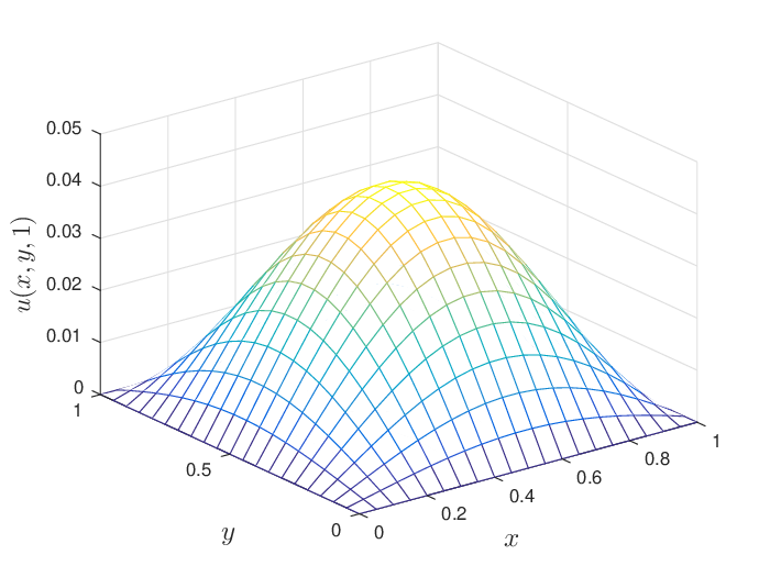
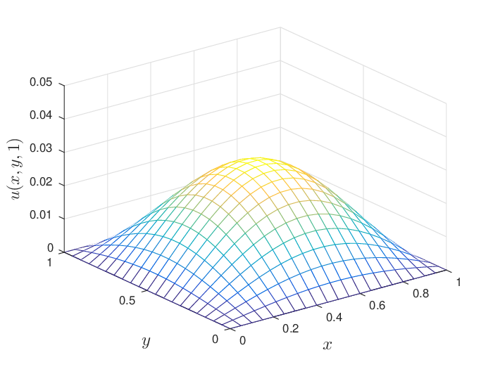
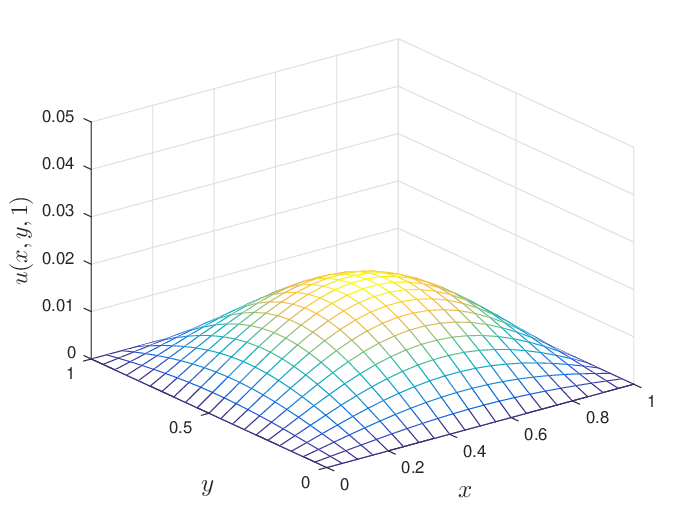
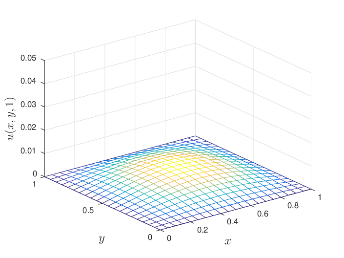
Finally we solve the time fractional diffusion equation

ut(α)​(x,y,t)+ux​(x,y,t)+uy​(x,y,t)=Δ​u​(x,y,t),u_{t}^{(\alpha)}(x,y,t)+u_{x}(x,y,t)+u_{y}(x,y,t)=\Delta u(x,y,t),\\

on the finite square domain Ω=(0,1)×(0,1)\Omega=(0,1)\times(0,1) for 0≤t≤10\leq t\leq 1, with the initial condition

u⁡(x,y,0)=sin⁡π​x​sin⁡π​y,for ​(x,y)∈Ω,u(x,y,0)=\sin\pi x\sin\pi y,\qquad\mbox{for }(x,y)\in\Omega,

and the boundary condition

u⁡(x,y,t)=0,(x,y)∈∂Ω×(0,1].u(x,y,t)=0,\qquad(x,y)\in\partial\Omega\times(0,1].

Figure 1 illustrates the computed solutions for t=1t=1 for several values of α\alpha. No exact solutions are known for this problem but the pictures illustrate the continuous dependence of the solutions on the fractional differentiation order.

In summary, this paper introduces an implicit finite difference approximation for the solution of an initial boundary value problem for a two dimensional time fractional advection-dispersion equation with variable coefficients in which the fractional derivative is given in the sense of Caputo and the dispersion terms are in nondivergence form. Proofs of consistency, stability and convergence are included and so are illustrative numerical experiments. A useful feature of the paper is the computational framework based on matrices. Our scheme was successfully implemented for the solution of an inverse source problem in [3]. We certainly expect to develop other applications of this scheme in the near future.

Acknowledgments

The authors would like to acknowledge financial support by Universidad Nacional de Colombia through the research project with Hermes code 33154.

References

  • [1] A.T. Balasim and N.H.M. Ali. New group iterative schemes in the numerical solution of the two-dimensional time fractional advection-diffusion equation. Cogent Mathematics, 4:1412241, 2017.
  • [2] K. Diethelm. The analysis of fractional differential equations. Springer, 2010.
  • [3] M. D. Echeverry and C. E. Mejía. A two dimensional discrete mollification operator and the numerical solution of an inverse source problem. AXIOMS, 7(4):89, 2018.
  • [4] S. Fomin, V. Chugunov, and T. Hashida. Application of fractional differential equations for modeling the anomalous diffusion of contaminant from fracture into porous rock matrix with bordering alteration zone. Transp Porous Med, 81:187–205, 2010.
  • [5] A A Kilbas, H M Srivastava, and J J Trujillo. Theory and applications of fractional differential equations. Elsevier North-Holland, 2006.
  • [6] Y. Lin and C. Xu. Finite difference/spectral approximation for the time-fractional diffusion equation. Journal of Computational Physics, 225:1533–1552, 2007.
  • [7] C. E. Mejía and A. Piedrahita. Solution of a time fractional inverse advection-dispersion problem by discrete mollification. Revista Colombiana de Matemáticas, 51(1):83–102, 2017.
  • [8] K.B. Oldham and J. Spanier. The fractional calculus: theory and applications of differentiation and integration to arbitrary order. Dover, Mineola, 2006.
  • [9] I. Podlubny. Fractional differential equations. Academic Press, 1999.
  • [10] Yuanyang Qiao, Shuying Zhai, and Xinlong Feng. RBF-FD method for the high dimensional time fractional convection-diffusion equation. International Communications in Heat and Mass Transfer, 89:230–240, 2017.
  • [11] Y.-M. Wang and L. Ren. Efficient compact finite difference methods for a class of time-fractional convection-reaction-diffusion equations with variable coefficients. International Journal of Computer Mathematics, DOI:10.1080/00207160.2018.1437262, 2018.
  • [12] Linlin Zhao, Fawang Liu, and Vo V Anh. Numerical methods for the two-dimensional multi-term time-fractional diffusion equations. Computers & Mathematics with Applications, 74(10):2253–2268, 2017.
  • [13] Pinghui Zhuang and Fawang Liu. Finite difference approximation for two-dimensional time fractional diffusion equation. Journal of Algorithms & Computational Technology, 1(1):1–16, 2007.