A hybrid algorithm for the two-trust-region subproblem
Abstract
Two-trust-region subproblem (TTRS), which is the minimization of a general quadratic function over the intersection of two full-dimensional ellipsoids, has been the subject of several recent research. In this paper, to solve TTRS, a hybrid of efficient algorithms for finding global and local-nonglobal minimizers of trust-region subproblem and the alternating direction method of multipliers (ADMM) is proposed. The convergence of the ADMM steps to the first order stationary condition is proved under certain conditions. On several classes of test problems, we compare the new algorithm with the recent algorithm of Sakaue et. al’s [28] and Snopt software.
Keywords: Two-trust-region subproblem, Trust-region subproblem, Local non-global minimum, Alternating direction method of multipliers.
1 Introduction
This paper studies the two-trust-region subproblem (TTRS), which is the minimization of a general quadratic function over the intersection of two full-dimensional ellipsoids:
| (TTRS) | ||||
where is a symmetric matrix, is symmetric positive definite, and . If is positive semidefinite, then TTRS is solvable in polynomial time by second-order cone programming. Therefore, throughout this paper we assume is indefinite.
When , TTRS reduces to the well-known trust-region subproblem (TRS) that has been widely studied and efficient algorithms exist to solve it [1, 13]. However, the additional constraint makes TTRS more challenging than TRS. TTRS is originally introduced by Celis, Dennis, and Tapia [11] and called the CDT subproblem. Two algorithms have been suggested for the CDT subproblem under the assumption that the objective function is convex [39, 17]. Zhang proposed an algorithm for the CDT subproblem under the assumption that the optimal Lagrangian Hessian is positive semidefinite [42]. However, Yuan proved that the Hessian of Lagrangian for CDT subproblem may have one negative eigenvalue at global solution [40]. In 1994, Martínez proved the existence of at most one local non-global minimum (LNGM) for TRS, which in the case of feasibility for TTRS is a candidate for its optimal solution [24]. Peng and Yuan showed that the CDT subproblem can have a duality gap and studied its necessary and sufficient optimality conditions [23]. Later in 2000, Nesterov and Wolkowicz proved that the following semidefinite programming (SDP) relaxation is tight for TTRS if and only if the Hessian of Lagrangian is positive semidefinite at global solution [25]:
| (SDP) | ||||
In 2001, Chen and Yuan presented a sufficient condition under which the Lagrangian function of the CDT subproblem has positive semidefinite Hessian at optimal solution. Moreover, Ye and Zhang [41] showed that for general CDT subproblem with certain additional conditions, the SDP relaxation is tight in many cases. In 2005, Li and Yuan proposed an algorithm that finds a global solution of the CDT subproblem with no duality gap, i.e., the Hessian of Lagrangian is positive semidefinite at global solution. Beck and Eldar [5] used the complex valued SDP approach to come up with a similar sufficient condition to guarantee the positive semidefiniteness of the Hessian of the Lagrangian function at optimal solution. They reported that in their experiments on randomly generated instances, their sufficient condition was satisfied for the majority of instances. In 2009, Ai and Zhang [2] derived verifiable conditions to characterize when the CDT subproblem has no duality gap, which is equivalent to when the SDP relaxation of the CDT problem is tight. In 2013, Burer and Anstreicher [9] provided a tighter relaxation by adding second order cone constraints to the classical SDP relaxation, but the resulting problem still has a relaxation gap. Later in 2016, Yang and Burer [38] reformulated special case of the TTRS with two variables into an exact SDP formulation by adding valid constraints. In general, the complexity of the CDT subproblem had been open for a long time, until Bienstock [6] recently proved its polynomial-time solvability. Unfortunately, Bienstock’s polynomial-time algorithm does not appear to be very practical, because the polynomial-time feasibility algorithm looks difficult to implement. In the most recent research, Sakaue et. al [28] proposed a polynomial-time algorithm assuming exact eigenvalue computation. However, due to the high computational cost of their algorithm, they reported numerical results for only dimension .
In several recent research, Alternating Direction Method of Multipliers (ADMM) has been successfully used
to solve both convex and nonconvex optimization problems with convergence analysis to stationary solutions [3, 8, 16, 19, 22, 33, 37, 31]. Moreover, global and local non-global minimizers of TRS are potential candidates for the optimal solution of TTRS in the case of feasibility. Thus in this paper, we propose a hybrid of efficient algorithms for finding the global and local non-global minimizers of TRS and ADMM to solve TTRS[1, 32]. The rest of the paper is organized as follows. In Section 2, we review some results related to LNGM of TRS and optimality conditions for TTRS. In Section 3, we describe the hybrid algorithm and prove the convergence of ADMM steps to the first-order stationary point. Finally, we report numerical results for several classes of test problems in Section 4 to demonstrate the efficiency of hybrid algorithm
compared with the algorithm of Sakaue et. al [28] for small dimensions and Snopt for medium and large-scale problems.
Notations: The th eigenvalue of is denoted by , where
Also is the spectral decomposition of where and denotes the th column of . The orthogonal complement of is
and denotes the nullspace of .
2 LNGM of TRS and optimality conditions
2.1 LNGM of TRS
In this subsection, we review some results related to TRS. Consider the following TRS by removing the second constraint of TTRS:
| (1) |
If the global solution of (1) is feasible for TTRS, then it is also a global solution for it. Otherwise, (1) might have a LNGM that is feasible for TTRS and also a candidate for its global solution. In what follows, we review some results related to LNGM of (1).
Theorem 2.1 (Necessary Conditions for LNGM, [24])
Let be a LNGM of (1). Choose such that is orthogonal. Then there exists a unique such that
| (2) | ||||
Corollary 1 (Lemma 3.2, [24])
If is orthogonal to some eigenvectors corresponding to , then no LNGM exists.
Now let
For
Theorem 2.1 shows that equation is a necessary condition for an LNGM. Furthermore, using the eigenvalue decomposition of , we have
| (3) |
Equation (3) implies that the function is strictly convex on and so it has at most two roots in the interval , which leads to the following theorem.
Theorem 2.2 (Theorem 3.1, [24])
Based on this intuition, given an instance of TRS with global minimizer and LNGM , one can enforce another ellipsoid that cuts off but leaves feasible. For the resulting instance of TTRS, becomes a natural candidate for the optimal solution of TTRS, although points near that remain feasible are good candidates as well. In this paper, we take advantage of the efficient algorithm developed in [32] to find LNGM within the proposed hybrid algorithm in the next section.
It is worth noting that the TRS by removing the first constraint of TTRS is as following:
| (4) |
which can be easily transformed to (1) by change of variables.
2.2 Optimality conditions and strong duality for TTRS
Let be a local solution of TTRS that satisfies the linear independence constraint qualification (LICQ). Then there exists a pair of Lagrange multipliers satisfying the KKT conditions:
| (5) | ||||
where is the Hessian of the Lagrangian.
Theorem 2.3 ([7])
Let at the KKT point , both constraints of TTRS be active.
(a) If is positive definite in for some multipliers pair satisfying
the KKT conditions (5), then is a local minimizer of TTRS.
(b) If is a local minimizer of TTRS, then is positive semidefinite in for some multipliers
pair satisfying the KKT conditions (5).
The following theorem gives necessary optimality conditions for TTRS.
Theorem 2.4 (Theorem 4.3, [23])
Let be a global minimizer of TTRS. If satisfies LICQ, then there exist such that
and has at least nonnegative eigenvalues.
A sufficient condition for the optimality of minimizing a quadratic function over two quadratic inequality constraints, when one of them is strictly convex, is presented in Theorem 2.1 of [2]. Since TTRS is a special case, we immediately have the following theorem.
Theorem 2.5 (Theorem 2.5, [40])
Let be feasible for TTRS. If there are two multipliers such that
then is a global solution of TTRS.
Theorem 2.6
Proof
We now discuss special cases of TTRS where strong duality holds.
Theorem 2.7
Suppose that and such that for all , and . If and , then strong duality holds for TTRS.
Proof
Theorem 2.8
Suppose that and such that for all , and . If and , then any local minimum of TTRS is a global minimum.
Proof
Let be a local minimum of TTRS that satisfies LICQ. Then there exist two nonnegative multipliers and such that satisfy KKT conditions (5). From , and (6), we have
| (7) |
If , then the three smallest eigenvalues of are negative, which contradicts the second order necessary optimality condition for TTRS. Therefore, any local minimum of TTRS is a global minimum.∎
3 Hybrid algorithm
In this section, we present the hybrid algorithm for solving TTRS. Before starting the ADMM steps, the feasibility of TTRS and the feasibility of global solutions of (1) and (4) for TTRS are checked. The feasibility of TTRS is checked by solving the following TRS:
| (8) |
If , then TTRS is feasible, otherwise it is infeasible.
In the case of feasibility of TTRS, we check whether the optimal solution of TRS (1) and (4) are optimal for TTRS. To do so, consider the following sets:
Let be the optimal solution of TRS (1). If , then is a global minimizer of TTRS. Also if the optimal solution of TRS (4) belongs to , then it is optimal for TTRS.
It is worth mentioning that for (1) and (4) hard case may occur. Therefore, we should check whether these two problems have another optimal solution in the feasible region of TTRS. This procedure is discussed for (4) since (1) is a special case of (4).
Definition 1 ([1])
A TRS is ”hard case”, if , the largest generalized eigenvalue of the pencil .
Theorem 3.1 ([1])
A vector is an optimal solution to the TRS (4) if and only if there exists such that
| (9) | ||||
| (10) | ||||
| (11) | ||||
| (12) |
Theorem 3.2 ([1])
Suppose TRS (4) belongs to the ”hard case” and satisfies (9)-(12) with . Let and be a basis of that is -orthogonal, i.e., . For an arbitrary , define
Then is positive definite. Moreover, is the minimum-norm solution to the linear system in the -norm, that is,
| (13) |
Furthermore, there exists such that is a solution for TRS (4).
Now let be the set of optimal solutions of (4), where . To see whether there exists an optimal solution of TRS (4) that belongs to , it is sufficient to solve the following problem:
| (14) |
This is equivalent to the following problem:
Let be its optimal solution, and set . If , then it is an optimal solution of TTRS. The same procedure should be performed for TRS (1).
After the above discussion, if none of the optimal solutions of TRS (1) and (4) are feasible for TTRS, we move to the steps of ADMM steps. One can write TTRS in the following equivalent form:
| (15) | ||||
To define the ADMM steps, consider the following augmented Lagrangian for (15):
where ’s are Lagrange multipliers and is the penalty parameter. The ADMM steps for the given and are as follow [8]:
- •
Step 1:
- •
Step 2:
- •
Step 3: where is a constant.
In Step 1, we solve the following TRS:
| (16) | |||||
Let be the optimal solution of (16). In Step 2, we solve the following TRS:
| (17) | |||||
As we see, in each step, we need to solve a TRS for which efficient algorithms are available [1, 13].
—————————————————————————————————
Hybrid algorithm
—————————————————————————————————
Step 0-1: Check the feasibility of TTRS by solving (8). If then TTRS is infeasible, exit;
else go to Step 2.
Step 0-2: Solve both TRS (1) and (4).
If or , then exit with the global solution of TTRS;
else go to Step 3.
Step 0-3: Compute the LNGM of (1) and (4) if they exist. Keep them if they are feasible for TTRS.
ADMM steps:
Input parameters: , maxiter. Choose appropriate penalty parameter and . Set and choose appropriate
and
For maxiter do
Solve TRS (16) and let be its optimal solution.
Solve TRS (17) and let be its optimal solution.
If , then exit with as output.
end if
Set and
end for.
Choose as the best of ADMM steps and LNGM of (4) and (1) if they exist.
—————————————————————————————————–
In what follows, if the global minimum of TTRS is not the global or LNGM of TRS (1) or (4), we discuss the convergence of the ADMM steps
to the stationary point of TTRS. First we present the following lemma.
Lemma 1
Suppose that is bounded and Then
Proof
Since solves problem (17) at -th iteration and is a feasible direction with respect to the feasible region of (17), then
| (18) |
Moreover,
| (19) |
where the inequality follows from the definition of the smallest eigenvalue of , , and (18). We also have
| (20) |
as is the minimizer of . On the other hand
| (21) | |||||
Now using (18), (20), and (21) we have
| (22) | |||||
Since and are bounded, from Step 3 of ADMM iterations, is also bounded. Thus is bounded. Moreover, since by assumption then from (22), is a bounded series (in the sense that the sequence of partial sums is bounded) with nonnegative terms, thus it is convergent. Therefore Moreover since by assumption from the Step 3 we have Finally since
and we know then .∎
In what follows, the convergence of algorithm to the first-order stationary conditions is proved.
Theorem 3.3
Let be any accumulation point of generated by the ADMM steps. Then by boundedness of and satisfies the first-order stationary conditions.
Proof
Since is an accumulation point of , then there exists a subsequence that converges to . Now consider subproblems that should be solved in Steps 1 and 2 of ADMM iterations. Subproblem (16) in Step 1 is a convex quadratic optimization problem which its necessary and sufficient optimality conditions are as follow:
| (23) | |||
where is the Lagrange multiplier. Moreover, subproblem in Step 2 is a TRS with the following necessary and sufficient optimality conditions:
| (24) | |||
Now by taking the limit of both (23) and (24), we get
| (25) | |||
| (26) | |||
| (27) | |||
| (28) | |||
| (29) | |||
| (30) |
which with (26), (27) and (29), (30) are the first-order stationary conditions.∎
4 Numerical experiments
In this section, we present several classes of test problems to assess the performance of Hybrid algorithm for solving TTRS. For small dimension problems, we compare Hybrid algorithm with the SDP relaxation of TTRS and by Sakaue et. al’s algorithm [28]. For large-scale problems, we do comparison with Snopt through Tomlab as the software giving best results. All computations are performed in MATLAB R2015a on a 2.50 GHz laptop with 8 GB of RAM. To solve the SDP reformulation, we have used CVX 1.2.1. For all test problems, we set and . To solve the TRSs within the algorithm we have used the algorithm in [1] and to find the LNGM of TRS we have used the algorithm of [32]. Finally, we should note that results in tables are the average of 100 runs for each dimension.
Our numerical experiments led to the following starting point procedure for Hybrid algorithm. By considering , the parametric form of the TTRS is constructed as follows:
| (31) |
| (32) |
Let and be optimal solutions of (31) and (32), respectively. For large enough and , these solutions are feasible for TTRS. Now, consider the following starting point for Hybrid algorithm:
| (33) |
| Notation | Description |
|---|---|
| n | Dimension of problem |
| Den | Density of and |
| CPU | Run time |
| KKT | |
| L(1) | Number of times that LNGM of problem (1) is feasible for TTRS |
| L(4) | Number of times that LNGM of problem (4) is feasible for TTRS |
| Opt-2active | Number of times that both constraints of TTRS are active at optimality |
| Opt-L (1) | Number of times that LNGM of TRS (1) is optimal |
| Opt-L (4) | Number of times that LNGM of TRS (4) is optimal |
| Obj | |
| Objective value of Hybrid algorithm | |
| Objective value of Snopt solver of Tomlab | |
| Cv-Snopt | Number of times the feasibility of constraints is violated by Snopt |
- •
First class of test problems:
Here we consider two small dimensional examples.
Example 1: Consider the following problem which is taken from [9]:The optimal solutions are with the objective value . The SDP relaxation gives and by applying the approach of [10], one gets objective value . Our algorithm gives with objective value , from any starting point. Both LNGM and global solutions of TRS (1) and (4) are infeasible for TTRS.
Example 2: Consider the following problem where the two ellipsoids intersect at four points as shown in Figure 2:Both TRS (1) and (4) have no LNGM and their global optimal solutions are not feasible for TTRS. Thus the optimal solution of TTRS is on the intersection of two constraints i.e., one of the four points. The global solution is with objective value and two local solutions are where the Hessian of Lagrangian has one negative eigenvalue. Also, is the third local solution where Hessian of Lagrangian has two negative eigenvalues. Hybrid algorithm can converge to any of these points, depending on the starting point. However, if we consider as starting point from (33), Hybrid algorithm converges to .
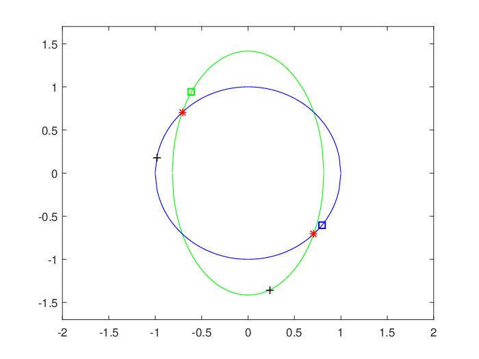
Figure 1: : global solution of (1) and (4), : local non-global solution of (1) and (4). : global solution of TTRS. The figure for Example 1 of First class. 
Figure 2: : global solution of (1) and (4), : local non-global solution of (1) and (4). : global solution of TTRS. : local solution with one negative eigenvalue at Hessian of Lagrangian. : local solution with two negative eigenvalue at Hessian of Lagrangian. : Starting point for Hybrid algorithm (given by (33)). - •
Second class of test problems
This class of test problems is generated using the following lemma [32].Lemma 2
Proof
To generate the desirable random instances of TTRS, we proceed as follows. First we construct a TRS instance of the form (1) having LNGM based on Lemma 2. Then we add the inequality constraint to enforce that the global minimizer of TRS be infeasible but the LNGM , , remains feasible (Figure 3) for TTRS. For of the generated instances, the LNGM of the TRS (4) is also in the feasible region of TTRS. Moreover, strong duality fails at of the generated instances.
For this class, we compare the Hybrid algorithm with Sakaue et. al’s algorithm [28] and the Snopt solver in Tomlab. Our extensive testing showed that , , and are appropriate choices where is given by (33). Results are summarized in Tables 2 to 4 for the average of 100 runs. In Table 2, we compare the Hybrid algorithm with the Sakaue et. al’s algorithm [28] for dimension . It can be seen that, Hybrid algorithm is much faster than Sakaue et. al’s algorithm while having equal objective values (the difference is of ) and comparable KKT accuracy[28]. In Tables 3 and 4, we compare Hybrid algorithm with the Snopt solver of Tomlab for different densities. From these two tables, we can conclude that Hybrid algorithm is much better than Snopt in large-scale problems. In Table 5, we have generated examples where the LNGM of TRS (4) is always feasible and for about of the generated instances, the LNGMs of TRS (1) are also feasible. Moreover, for over of instances, the optimal solution is at one of LNGM , mostly on LNGM of TRS (4).

Figure 3: : global solution of (4) and (1), : LNGMs of (1) and (4) . Hybrid algorithm Sakaue et. al algorithm [28] n Obj CPU KKT Obj CPU KKT 5 -132.94 1.52 1.23e-08 -132.94 0.04 1.47e-10 10 -144.27 1.85 5.15e-08 -144.27 0.57 1.73e-11 15 -139.85 2.19 3.50e-08 -139.85 8.75 1.74e-10 20 -114.12 2.17 6.49e-08 -114.12 49.02 1.16e-09 25 -114.64 2.33 1.17e-08 -114.64 186.34 2.20e-09 30 -134.51 2.81 6.54e-08 -134.51 597.72 9.57e-09 Table 2: Comparison with Sakaue et. al’s algorithm [28] when . n CPU(Hybrid algorithm) Cv-Snopt CPU(Snopt) 50 2.91 83 10 4 4.66 100 4.22 81 14 2 4.62 200 10.96 80 10 10 15.82 300 23.62 86 12 2 30.45 500 62.32 82 16 0 70.43 Table 3: Comparison with Snopt solver of Tomlab when . n CPU(Hybrid algorithm) Cv-Snopt CPU(Snopt) 100 1.89 71 26 0 3.14 200 3.35 86 12 1 11.51 300 3.88 78 19 3 19.63 500 7.35 80 19 0 52.27 700 18.88 76 21 3 107.36 1000 30.62 75 19 3 233.92 2000 241.68 67 22 10 1429.76 Table 4: Comparison with Snopt solver of Tomlab when . - •
ُThird class of test problems
In this class, we generate TTRS instances where LNGMs and global minimizers of (1) and (4) are all infeasible for TTRS. This is done in two ways. In the first method, matrix is generated such that the multiplicity of it’s minimum eigenvalue is at least two. Thus TRS has no LNGM . The second method is based on Corollary 1. Moreover, in this class, strong duality holds for at least of the generated instances. Starting point for Hybrid algorithm uses (33) and according to our extensive testing , , and are appropriate choices. Results are summarized in Tables 6 and 7 for the average of 100 runs. In dimensions to , we compare Hybrid algorithm with the Sakaue et. al’s algorithm [28], the corresponding results are reported in Table 6. As we see, our method has significant advantages over the Sakaue et. al’s algorithm [28] in term of CPU time while having equal objective values and comparable KKT accuracies. In Table 7, we compare the Hybrid algorithm with the Snopt solver in Tomlab. The Snopt for is better in term of CPU time but for larger dimensions Hybrid algorithm has better time performance. It is worth to note that the optimal values for both methods are almost the same for most of the problems as shown in the third column of Table 7.Hybrid algorithm Sakaue et. al algorithm [28] n Obj CPU KKT Obj CPU KKT 5 -38.31 0.41 6.32e-08 -38.31 0.03 1.92e-10 10 -48.94 1.06 5.81e-08 -48.94 0.49 1.08e-09 15 -57.29 1.11 5.15e-08 -57.29 7.77 1.73e-11 20 -68.56 0.98 4.72e-08 -68.56 46.08 1.71e-12 25 -75.38 1.06 4.43e-08 -75.38 188.56 7.63e-12 30 -16.42 1.67 4.21e-10 -16.42 710.52 7.28e-15 Table 6: Comparison with Sakaue et. al’s algorithm [28] when . n Den CPU(Hybrid algorithm) Cv-Snopt CPU(Snopt) 50 1 2.96 96 2 2 6.31 100 1 6.31 97 3 0 5.34 200 1 22.57 88 10 2 18.33 300 1 74.92 82 13 5 55.05 500 0.1 6.16 98 0 2 45.77 700 0.1 7.58 98 0 2 80.77 800 0.1 9.13 95 2 3 112.93 900 0.1 10.84 95 1 4 134.25 1000 0.1 11.07 95 0 5 178.83 Table 7: Comparison of Hybrid algorithm with Snopt solver of Tomlab. - •
Forth class of test problems( Homogeneous problem)
For this class, we consider and in TTRS. Consequently, strong duality holds and thus SDP relaxation of TTRS is exact [41]. Since the optimal solution of Hybrid algorithm satisfies the conditions of Theorem 2.5, it results in the optimal solution of TTRS. In this class, we compare the Hybrid algorithm in terms of CPU time and objective value with CVX software solving SDP relaxation. We set , and , where is given by (33). The results are summarized in Table 8 for the average of 100 runs. As we see, for CVX is faster, while both have the same optimal objective value. However, for , Hybrid algorithm solves the problem to global optimality while CVX can not be applied.Hybrid algorithm SDP n Den Obj CPU KKT Obj CPU 50 1 -37.93 5.41 4.9e-08 -37.93 0.58 100 1 -57.84 10.34 8.53e-08 -57.84 1.16 300 1 -100.70 95.93 1.08e-08 -100.70 15.44 500 0.1 -42.94 57.23 9.94e-08 -42.94 27.16 700 0.1 -49.75 116.31 9.94e-08 -49.75 70.58 1000 0.1 -56.98 241.89 2.25e-08 -56.98 366.64 2000 0.01 -28.48 162.45 5.17e-08 3000 0.001 -15.39 57.35 1.28e-08 4000 0.001 -19.29 140.63 6.29e-08 5000 0.001 -16.21 209.17 1.01e-08 Table 8: Comparison of Hybrid algorithm with CVX.
5 Conclusions
In this paper, a hybrid algorithm which take advantages of efficient algorithms for finding global and local non-global minimizers of TRS and alternating direction method of multipliers (ADMM) is proposed to tackle the two-trust-region subproblem. The convergence of ADMM steps to the first-order stationary condition is proved. Our numerical experiments on several classes of test problems show that for small-scale problems hybrid algorithm has better performance in overall compared to the polynomial-time algorithm of Sakaue et. al’s [28]. Moreover, on medium and large-scale problems comparison with Snopt from Tomlab, as the software giving best results, show that in term of running time, hybrid algorithm is better. Also for large-scale homogeneous problems, hybrid algorithm outperforms CVX software.
References
- (1) S. Adachi, S. Iwata, Y. Nakatsukasa and A. Takeda, Solving the trust region subproblem by a generalized eigenvalue problem, Mathematical Engineering Technical Report(METR 2015-14), Department of Mathematical Informatics, Graduate School of Information Science and Technology, The University of Tokyo.
- (2) W. Ai and S. Zhang. Strong duality for the CDT subproblem: a necessary and sufficient condition. SIAM J. Optim., 19(4): 1735-1756, 2008.
- (3) X. Bai and K. Scheinberg, Alternating direction methods for non convex optimization with applications to second-order least-squares and risk parity portfolio selection, Optimization-Online, 2015.
- (4) X. Bai, J. Sun, S. Sun and X. Zheng, An alternating direction method for chance-constrained optimization problems with discrete distributions. Optimization-Online, 2012.
- (5) A. Beck and Y.C. Eldar, Strong duality in nonconvex quadratic optimization with two quadratic constraints, SIAM Journal on Optimization, 17(3), 844-860, 2006.
- (6) D. Bienstock, A note on polynomial solvability of the CDT problem, preprint, SIAM J. Optim., pp. 488-498, 2016.
- (7) Im. Bomze, Ml. Overton, Narrowing the difficulty gap for the Celis-Dennis-Tapia problem, Mathematical Programming 151.2, 459-476, 2015.
- (8) S. Boyd, N. Parikh, E. Chu, B. Peleato and J. Eckstein, Distributed optimization and statistical learning via the alternating direction method of multipliers, Foundations and Trends in Machine Learning, 3(1), 1-122, 2011.
- (9) S. Burer and K.M. Anstreicher, Second-order-cone constraints for extended trust-region subproblems, SIAM Journal on Optimization, 23(1), 432-451, 2013.
- (10) S. Burer and B. Yang, The trust region subproblem with non-intersecting linear constraints, Mathematical Programming 149, 253-264, 2015.
- (11) M.R. Celis, J.E. Dennis, R.A. Tapia, A trust region algorithm for nonlinear equality constrained optimization, in Numerical Optimization, R.T. Boggs, R.H. Byrd, and R.B. Schnabel, eds., SIAM, Philadelphia, pp. 71-82, 1984.
- (12) X. Chen, Y. Yuan, On maxima of dual function of the CDT subproblem, J. Comput. Math, pp. 113-124, 2000.
- (13) A.R. Conn, N.I. Gould and P. L. Toint, Trust Region Methods, SIAM, Philadelphia, PA, 2000.
- (14) M. Grant and S. Boyd. CVX: Matlab software for disciplined convex programming, version 2.0 beta. http://cvxr.com/cvx, September 2013.
- (15) C. Fortin and H. Wolkowicz, The trust region subproblem and semidefinite programming, Optimization Methods and Software, 19(1), 41-67, 2004.
- (16) D. Hajinezhad and Q. Shi, Alternating direction method of multipliers for a class of nonconvex bilinear optimization: convergence analysis and applications, Journal of Global Optimization, 70(1), 261-288, 2018.
- (17) M. Heinkenschloss, On the solution of a two ball trust region subproblem, Mathematical Programming, 249-276, 1994.
- (18) Y. Hsia and R. L. Sheu, Trust region subproblem with a fixed number of additional linear inequality constraints has polynomial complexity, arXiv preprint arXiv, 1312.1398, 2013.
- (19) M. Hong, Z.Q. Luo and M. Razaviyan, Convergence analysis of alternating direction method of multipliers for a family of nonconvex problems. SIAM Journal on Optimization, 26(1), 337-364, 2016.
- (20) V. Jeyakumar and G. Y. Li, Trust-region problems with linear inequality constraints: exact SDP relaxation, global optimality and robust optimization, Mathematical Programming 147, 171-206, 2014.
- (21) E. de Klerk, C. Roos, T. Terlaky, Nonlinear Optimization (CO 367). Waterloo, 2006.
- (22) H. Luo, X. Sun and H. Wu, Convergence properties of augmented Lagrangian methods for constrained global optimization, Optimization Methods and Software, 23(5), 763-778, 2008.
- (23) J.-M. Peng, Y. Yuan, Optimality conditions for the minimization of a quadratic with two quadratic constraints, SIAM Journal on Optimization, 7 (1997),
- (24) J.M. Martinez, Local minimizers of quadratic functions on Euclidean balls 336 and spheres. SIAM Journal on Optimization, 4(1), 159-176, 1994.
- (25) Y. Nesterov, H. Wolkowicz, Y. Ye, Semidefinite programming relaxations of nonconvex quadratic optimization, Handbook of semidefinite programming. Springer, Boston, 361-419, 2000.
- (26) M. J. D. Powell and Y. Yuan, A trust-region algorithm for equality constrained optimization, Math. Program., pp. 189-211, 1991.
- (27) F. Rendl and H. Wolkowicz, A semidefinite framework for trust region subproblems with applications to large scale minimization, Mathematical Programming, 77(1), 273-299, 1997.
- (28) S. Sakaue, Y. Nakatsukasa, A. Takeda, and S. Iwata, Solving generalized CDT problems via two-parameter eigenvalues, SIAM Journal on Optimization, 26(3), 1669-1694, 2016.
- (29) M. Salahi and S. Fallahi, Trust region subproblem with an additional linear inequality constraint, Optimization Letters, 10(4), 821-832, 2016.
- (30) M. Salahi and A. Taati, A fast eigenvalue approach for solving the trust region subproblem with an additional linear inequality, Computational and Applied Mathematics37.1 (2018): 329-347
- (31) M. Salahi, and A. Taat, Alternating direction method of multipliers for the extended trust region subproblem, Iranian Journal of Numerical Analysis and Optimization 7.1 (2017): 107-117.
- (32) M. Salahi, A. Taati, H. Wolkowicz, Local nonglobal minima for solving large scale extended trust region subproblems. Computational Optimization and Applications. 2016.
- (33) Y. Shen, Z. Wen and Y. Zhang, Augmented Lagrangian alternating direction method for matrix separation based on low-rank factorization, Optimization Methods Software, 29(2), 239-263, 2014.
- (34) J.F. Sturm and S. Zhang, On cones of nonnegative quadratic functions, Mathematics of Operations Research, 28(2), 246-267, 2003.
- (35) Y.-X. Yuan, On a subproblem of trust region algorithms for constrained optimization, Mathematical Programming, 1990.
- (36) Y. Xu, W. Yin, Z. Wen and Y. Zhang, An alternating direction algorithm for matrix completion with nonnegative factors, Journal of Frontiers of Mathematics in China, Special Issues on Computational Mathematics, 365-384, 2011.
- (37) L. Xu, B. Yu, and Y. Zhang, An alternating direction and projection algorithm for structure-enforced matrix factorization, Computational Optimization and Applications, 68(2), 33-362, 2017.
- (38) B. Yang, S. Burer, A two-variable approach to the two-trust-region subproblem, SIAM J. Optim., pp. 661-680, 2016.
- (39) Y. Yuan, A dual algorithm for minimizing a quadratic function with two quadratic constraints, J. Comput. Math., , pp. 348–359. 1991.
- (40) Y. Yuan, On a subproblem of trust region algorithms for constrained optimization, Math. Program, pp. 53-63, 1990.
- (41) Y. Ye and S. Zhang, New results on quadratic minimization, SIAM Journal on Optimization, pp. 245-267. 2003.
- (42) Y. Zhang, Computing a Celis-Dennis-Tapia trust-region step for equality constrained optimization, Math. Program, pp. 109-124, 1992.