Rotating traversable wormholes in AdS

One key ingredient to study traversability is the knowledge of the bulk-to-boundary propagator. Since the rotating BTZ solution is locally $AdS_{3}$, the bulk-to-boundary propagator can be obtained from the propagator for $AdS_{3}$ via a coordinate transformation. The result when both bulk and boundary points are contained in region $1_{++}$ is [21],

		$\displaystyle\mathcal{K}(z,t,x;t_{1},x_{1})=$
		$\displaystyle\quad\frac{(r_{+}^{2}-r_{-}^{2})^{\frac{\Delta}{2}}}{2^{\Delta+1}\pi\ell}\sum_{n={-\infty}}^{\infty}\left[-\sqrt{z-1}\cosh\left(\kappa\delta t-\frac{r_{-}}{\ell}\delta x_{n}\right)+\sqrt{z}\cosh\left(\frac{r_{+}}{\ell}\delta x_{n}\right)\right]^{-\Delta},$		(3.4)

where

$$z=\frac{r^{2}-r_{-}^{2}}{r_{+}^{2}-r_{-}^{2}},\quad\delta t=t-t_{1},\quad\text{and}\quad\delta x_{n}=x-x_{1}+2\pi n.$$

(3.5)

Note that the overall normalization of the propagator is obtained by taking the limit to the boundary from the bulk-to-bulk propagator [25, 26], such that it agrees with the propagator considered by GJW in the limit $r_{-}\to 0$. Near the event horizon in the region $1_{++}$, it is possible to explicitly invert the Kruskal coordinates (2.8) to obtain

$$t=\frac{1}{2\kappa}\log\left(-\frac{U}{V}\right),\qquad z=1-\gamma^{2}\,UV+O(U^{2}V^{2}),$$

(3.6)

where we have defined

$$\gamma^{2}\equiv\Omega^{2}(r=r_{+})=\frac{4r_{+}^{2}\ell^{2}}{r_{+}^{2}-r_{-}^{2}}\left(\frac{r_{+}-r_{-}}{r_{+}+r_{-}}\right)^{r_{-}/r_{+}}.$$

(3.7)

For example, the bulk-to-boundary propagator along $V=0$ for both points contained in region $1_{++}$ becomes (omiting sum over images)

$$\mathcal{K}(U,0,x;\,U_{1},x_{1})=\frac{\left(r_{+}^{2}-r_{-}^{2}\right)^{\frac{\Delta}{2}}}{2^{\Delta+1}\pi\ell}\left(\frac{1}{-\frac{\gamma}{2}U/U_{1}e^{-r_{-}(x-x_{1})}+\cosh[r_{+}(x-x_{1})]}\right)^{\Delta},$$

(3.8)

and propagators for points in different regions can be obtained using the imaginary shifts in time that we have described in Sec. 2. We will also need the retarded bulk-to-boundary propagator, which can be expressed as

		$\displaystyle\mathcal{K}_{\text{ret}}(z,t,x;t_{1},x_{1})=$		(3.9)
		$\displaystyle=|\mathcal{K}(z,t,x;t_{1},x_{1})|\,\theta(\delta t)\,\theta\left(\sqrt{z-1}\cosh\left(\kappa\,\delta t-\frac{r_{-}}{\ell}\delta x\right)-\sqrt{z}\cosh\left(\frac{r_{+}}{\ell}\delta x\right)\right).$

Throughout the rest of the paper we will set $\ell=1$ for simplicity.

We now evaluate the modified stress tensor in the rotating BTZ background when we turn on the interaction (3.2). The analytic continuation of the bulk-to-boundary propagator when the points are time-like separated from the boundary was studied in [24]. This continuation works very much like in the non-rotating case. Therefore, the steps of the calculation follow closely [4].

The starting point is to evaluate the bulk two-point function

$$G(U,U^{\prime})\equiv{\left<{\Phi_{R}(U,x)\Phi_{R}(U^{\prime},x)}\right>}.$$

(3.10)

In the perturbative expansion in the coupling $h$, the one-loop contribution to the two-point function is

$$G_{h}=\frac{2h\sin(\pi\Delta)}{\kappa^{2\Delta-2}}\int_{t_{0}}^{t_{f}}dt_{1}dx_{1}\mathcal{K}(r^{\prime},t^{\prime},x^{\prime};-t_{1}+i\tfrac{\beta}{2},x_{1})\mathcal{K}_{\text{ret}}(r,t,x;t_{1},x_{1})+(t\leftrightarrow t^{\prime}),$$

(3.11)

where we used the imaginary shift $t\to t-i\beta/2$ to move all the points to the right region $1_{++}$. Using the propagators (3.4) and (3.9), and evaluating at $V=0$ in Kruskal coordinates gives

		$\displaystyle G_{h}(U,U^{\prime})=$
		$\displaystyle C_{0}\int_{U_{0}}^{U}\frac{dU_{1}}{U_{1}}\left(\frac{1}{\frac{\gamma}{2}e^{-r_{-}\delta x}U_{1}U^{\prime}+\cosh(r_{+}\delta x)}\right)^{\Delta}\left(\frac{U_{1}}{\frac{\gamma}{2}e^{-r_{-}\delta x}U-U_{1}\cosh(r_{+}\delta x)}\right)^{\Delta}dx_{1}$
		$\displaystyle\hskip 361.34999pt+(U\leftrightarrow U^{\prime})$		(3.12)

where $U_{0}=e^{\kappa\,t_{0}}$. After we shut down the interaction ($U>U_{f}=e^{\kappa\,t_{f}}$) the upper limit in the $U_{1}$ integral should be replaced by $U_{f}$. The overall constant is

$$C_{0}=\frac{h\kappa^{1-\Delta}r_{+}^{\Delta}\sin(\Delta\pi)}{2(2^{\Delta}\pi)^{2}}.$$

(3.13)

The sum over the images extends the domain of the $x_{1}$ integral to the entire real axis, but it ends being constrained by the $\theta-$function in the retarded propagator (3.9), which requires that

$$\frac{\gamma}{2}\,e^{-r_{-}\delta x}U-U_{1}\cosh(r_{+}\delta x)\geq 0.$$

(3.14)

The bulk stress tensor associated to the scalar field $\Phi$ is

$$T_{\mu\nu}=\partial_{\mu}\Phi\partial_{\nu}\Phi-\frac{1}{2}g_{\mu\nu}g^{\rho\sigma}\partial_{\rho}\Phi\partial_{\sigma}\Phi-\frac{1}{2}g_{\mu\nu}m^{2}\Phi^{2}.$$

(3.15)

At one-loop, the expectation value of the stress tensor for the perturbed Hamiltonian can be evaluated via point splitting

$${\left<{T_{\mu\nu}}\right>}=\lim_{{\rm x}\to{\rm x}^{\prime}}\left(\partial_{\mu}\partial_{\nu}G({\rm x},{\rm x}^{\prime})-\frac{1}{2}g_{\mu\nu}g^{\rho\sigma}\partial_{\rho}\partial_{\sigma}G({\rm x},{\rm x}^{\prime})-\frac{1}{2}g_{\mu\nu}m^{2}G({\rm x},{\rm x}^{\prime})\right).$$

(3.16)

When evaluated along the horizon at $V=0$, the $g_{UU}$ component of the unperturbed metric vanishes, so the leading contribution to the null component of the stress tensor is,

$$T_{UU}=\lim_{U^{\prime}\to U}\partial_{U}\partial_{U^{\prime}}G_{h}(U,U^{\prime}).$$

(3.17)

where the perturbed propagator $G_{h}(U,U^{\prime})$, obtained in (3.12), can be evaluated numerically. Evaluating (3.17) we can find the effect of the double trace deformation on the average null energy. As we see in Fig. 2 our results show that the ANEC is violated.

As mentioned in Sec. 1, ANEC violation is a necessary condition for a wormhole becoming traversable. It is illuminating to explicitly follow a null ray in the perturbed metric going from past infinity ($U\rightarrow-\infty$) to future infinity ($U\rightarrow\infty$) along the $V=0$ horizon. The linearized Einstein equation for the $UU$ component for the fluctuations evaluated at $V=0$ gives

$$\int dU\left(\frac{\kappa}{2r_{+}}h_{UU}-\frac{r_{-}\partial_{x}h_{UU}}{r_{+}^{2}}-\frac{\partial_{x}^{2}h_{UU}}{2r_{+}^{2}}\right)=8\pi G_{N}\int dUT_{UU},$$

(3.18)

where we assume that the fluctuations vanish at infinity. Since the interaction (3.2) is being integrated over the transverse space, the modified stress tensor should be independent of the transverse coordinate $x$. This reduces the equation to

$$8\pi G_{N}\int dUT_{UU}=\frac{\kappa}{2r_{+}}\int dUh_{UU}=\frac{r_{+}^{2}-r_{-}^{2}}{2r_{+}^{2}}\int dUh_{UU}.$$

(3.19)

We can now relate the average null energy to the shift $\Delta V(U)$ in the null geodesics at the horizon caused by the interaction. After including the perturbation, we can see from the metric (2.9) that the null ray originating in the past is given by,

$\displaystyle\Delta V(U)$

$\displaystyle=-\frac{1}{2g_{UV}(0)}\int_{-\infty}^{U}dUh_{UU}$

(3.20)

where $g_{UV}(0)$ is the $U\,V$ component of the original metric evaluated on $V=0$. Now, from (3.19) and (3.20) we get,

$$\Delta V(U)=\frac{1}{2}\left(\frac{r_{+}-r_{-}}{r_{+}+r_{-}}\right)^{-\frac{r_{-}}{r_{+}}}8\pi G_{N}\int_{-\infty}^{U}dUT_{UU}.$$

(3.21)

We identify the “size” of opening of the wormhole as $\Delta V(\infty)$, which we will denote simply by $\Delta V$.

In [6] the authors elaborated on the quantum information interpretation of the results in [4]. Focusing on nearly $AdS_{2}$ gravity [27], which is claimed to be the dual of the SYK model, they presented a bound on the information that can be transferred through the wormhole. They also considered a double trace deformation⁴⁴ 4 More precisely, they considered the slightly different interaction $\frac{g}{K}\sum_{j=1}^{K}\mathcal{O}^{j}_{R}(0)\mathcal{O}^{j}_{L}(0)$, where the $K$ fields are introduced to make the effect larger and the interaction is turned on only at time $t=0$. but proposed a different way to diagnose traversability of the wormhole using techniques involving out-of-time order correlation functions that appear in the context of quantum chaos [28, 29]. In this perspective, traversability can be interpreted as the result of a high energy scattering where the signal particle $\phi$ scatters with $\mathcal{O}$ and suffers a time advance for positive $h$, so it can emerge on the other boundary (Fig. 7).

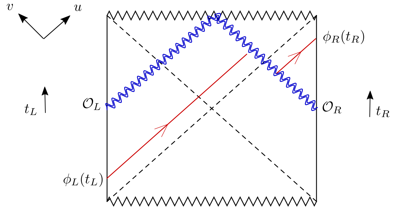
In this section we review the diagnose of [6] and we adapt their results to derive the opening of the wormhole for the eternal rotating BTZ black hole. We consider a generic metric in Kruskal coordinates written as

$$ds^{2}=-a(uv)dudv+\left(b(u,v)du+c(u,v)dv+r(uv)dx\right)^{2},$$

(4.1)

and let us define the following quantities evaluated at the horizon

$$\quad a_{0}=a(0),\quad r_{0}=r(0).$$

(4.2)

We will assume that $b(v=0)=0$ to simplify the calculation. Note that this applies to the rotating BTZ case (2.9). In the framework of [6] the diagnose of traversability is based on the commutator

$${\left<{\left[\phi_{L},e^{-i\mathcal{V}}\phi_{R}\,e^{i\mathcal{V}}\right]}\right>},\qquad\mathcal{V}\equiv\int_{t_{0}}^{t}dt_{1}\,\delta H(t_{1}),$$

(4.3)

where $\phi_{R}=\phi_{R}(t_{R})$, $\phi_{L}=\phi_{L}(t_{L})$, and the brackets ${\left<{...}\right>}$ denote the expectation value in the TFD state. The convention for time is $t_{R}=-t_{L}=t$. If the commutator is non-zero, then the signal from the left boundary successfully reached the right boundary.

Assuming the operators are Hermitian, we can focus on a simpler quantity

$$C\equiv{\left<{e^{-i\mathcal{V}}\phi_{R}\,e^{i\mathcal{V}}\phi_{L}}\right>},$$

(4.4)

which is related to the original commutator via

$${\left<{\left[\phi_{L},e^{-i\mathcal{V}}\phi_{R}\,e^{i\mathcal{V}}\right]}\right>}=-2\,\text{Im}(C).$$

(4.5)

In the small $G_{N}$ limit, and assuming the relative boost between $\mathcal{O}$ and $\phi$ is large, we can approximate the scattering between states created by $\phi$ and $\mathcal{O}$ by a shock wave with amplitude $S_{\text{grav}}=e^{i\tilde{\delta}}$ [30, 31]. The final expression is [6] (see also [13])

$$C=e^{i{\left<{\mathcal{V}}\right>}}\alpha\int dp^{u}\,dy\,p^{u}\Psi_{\phi_{L}}^{*}(p^{u},y)\Psi_{\phi_{R}}(p^{u},y)\,e^{i\mathcal{D}},$$

(4.6)

where $\alpha=\frac{a_{0}^{2}r_{0}}{4\pi}$. The exponent is defined by

$$\mathcal{D}\equiv\alpha\int dq^{v}\,dx\int dt_{1}\,dx_{1}\,q^{v}e^{i\tilde{\delta}}h(t_{1},x_{1})\Psi_{\mathcal{O}_{R}}^{*}(q^{v},x)\Psi_{\mathcal{O}_{L}}(q^{v},x),$$

(4.7)

where the wavefunctions are given by the Fourier transform of the bulk-to-boundary propagators

	$\displaystyle\Psi_{\mathcal{O}_{R}}(q^{v},x)$	$\displaystyle=\int dve^{ia_{0}q^{v}v/2}{\left<{\Phi(u,v,x)\,\mathcal{O}_{R}^{\dagger}(t_{1},x_{1})}\right>}_{u=0},$
	$\displaystyle\Psi_{\mathcal{O}_{L}}(q^{v},x)$	$\displaystyle=\int dve^{ia_{0}q^{v}v/2}{\left<{\Phi(u,v,x)\,\mathcal{O}_{L}(-t_{1},x_{1})}\right>}_{u=0},$
	$\displaystyle\Psi_{\phi_{R}}(p^{u},y)$	$\displaystyle=\int due^{ia_{0}p^{u}u/2}{\left<{\Phi_{\phi}(u,v,y)\,\phi_{R}(t,y_{1})}\right>}_{v=0},$
	$\displaystyle\Psi_{\phi_{L}}(p^{u},y)$	$\displaystyle=\int due^{ia_{0}p^{u}u/2}{\left<{\Phi_{\phi}(u,v,y)\,\phi_{L}^{\dagger}(-t,y_{1})}\right>}_{v=0},$		(4.8)

and $\Phi_{\phi}$ is the bulk field dual to $\phi$. In the above expression, we have decomposed the single particle wavefunction of $\phi$ into states with momentum $p^{u}$ on the $v=0$ slice, and momentum $q^{v}$ on the $u=0$ slice for $\mathcal{O}$. The operator $\mathcal{O}_{L/R}$ is applied at a point $x_{1}$ and $\phi_{L/R}$ is applied at $y_{1}$ in transverse space, while $x$ and $y$ are bulk transverse coordinates that appear in the bulk-to-boundary propagators being integrated.

Here we derive the opening of the wormhole for rotating BTZ using the formula (4.6) in the probe limit. The first step is to derive the scattering amplitude $e^{i\tilde{\delta}}$, which can be found by studying particles propagating along the horizon whose effect is to produce a shock wave geometry [29]. For simplicity, let us assume the matter creating the shock wave is symmetrically distributed over the transverse space, so that the scattering amplitude will be independent of the transverse coordinates.

The parameters (4.2) for the rotating BTZ metric (2.9) are identified as

$$a_{0}=\gamma^{2},\qquad r_{0}=r_{+},$$

(4.9)

with $\gamma$ defined as in (3.7). If we send the matter with momentum $p_{v}$ along $v=0$, this corresponds to a stress tensor⁵⁵ 5 Upper and lower indices are related by $q^{v}=-\frac{2}{a_{0}}q_{u}$, $p^{u}=-\frac{2}{a_{0}}p_{v}$.

$$T_{vv}=\frac{-p_{v}}{r_{+}L}\delta(v),\quad\text{so that}\quad-p_{v}=\int r_{+}dx\,dvT_{vv},$$

(4.10)

where $L$ denotes the integral of the transverse coordinate without the measure factor $r_{+}$. For rotating BTZ we have $L=2\pi$, but we keep this factor general to make the dependence on the volume of the transverse space explicit. From the linearized Einstein equations (3.19) for the $vv$ component, we have

$$8\pi G_{N}T_{vv}=\frac{\kappa}{2r_{+}}h_{vv},$$

(4.11)

which gives

$$h_{vv}=a_{0}a^{u}\delta(v),\quad a^{u}\equiv-\frac{16\pi G_{N}}{a_{0}\kappa L}p_{v}.$$

(4.12)

The effect is then to produce a translation by an amount $a^{u}$ once we cross the horizon $v=0$. Note that $a^{u}>0$ since $p_{v}$ is negative for a physical particle. The scattering amplitude is identified as

$$i\tilde{\delta}=-ia^{u}q_{u}.$$

(4.13)

In the probe limit, in which we assume $a^{u}$ is small, we can expand the exponent in (4.7) for small $a^{u}$. The zeroth order term of the expansion cancels with $e^{i{\left<{\mathcal{V}}\right>}}$ in the expression for $C$ (4.6), while the term proportional to $a^{u}$ contributes to a term that acts as a translation for the $\phi$ wavefunction. In the end we obtain a correlator for $\phi$ that has the form

$$C_{\text{probe}}={\left<{\phi_{R}e^{-ia^{v}\hat{P}_{v}}\phi_{L}}\right>},$$

(4.14)

where

$$a^{v}=-\frac{i\alpha}{p^{u}}\int dq^{v}\,dx\int dt_{1}\,dx_{1}\,q^{v}\,\tilde{\delta}\,h(t_{1},x_{1})\Psi_{\mathcal{O}_{R}}^{*}(q^{v},x)\Psi_{\mathcal{O}_{L}}(q^{v},x),$$

(4.15)

and $\hat{P}_{v}$ is the translation operator that shifts the $\phi_{L}$ wavefunction by an amount $a^{v}$ along the $v$ direction. This gives us the opening of the wormhole in the probe limit that was calculated using a different method in Sec. 3.2. The quantity $a^{v}$ here corresponds to $\Delta V$ in (3.21).

Let us evaluate (4.15) for the rotating BTZ. The wavefunctions $\Psi_{\mathcal{O}_{L/R}}$ can be computed explicitly since we know the form of the bulk-to-boundary propagator, which evaluated at $u=0$ is

$$\mathcal{K}(0,v,x;t_{1},x_{1})=\frac{\left(r_{+}^{2}-r_{-}^{2}\right)^{\frac{\Delta}{2}}}{2^{\Delta+1}\pi}\left(\frac{1}{-v\frac{\gamma}{2}e^{-r_{-}(x-x_{1})}e^{-\kappa t_{1}}+\cosh[r_{+}(x-x_{1})]}\right)^{\Delta}.$$

(4.16)

By performing the Fourier transform we obtain the wavefunctions

		$\displaystyle\Psi_{\mathcal{O}_{L}}(q^{v},x)=\tfrac{2^{1+\Delta}q^{v}(q^{v}\gamma)^{-2+\Delta}(r_{+}\kappa)^{\Delta/2}}{\Gamma(\Delta)}e^{i\cosh[r_{+}(x-x_{1})]e^{-r_{-}(x-x_{1})\kappa t_{1}}q^{v}\gamma-\frac{i\pi\Delta}{2}-r_{-}\Delta(x-x_{1})+\kappa t_{1}},$
		$\displaystyle\Psi^{*}_{\mathcal{O}_{R}}(q^{v},x)=\Psi_{\mathcal{O}_{L}}(q^{v},x)|_{t_{1}\to-t_{1}}.$		(4.17)

We can evaluate (4.15) by performing the integral over $q^{v}$ first. The integral over $x_{1}$ is extended over all real axis because we are summing over the contribution of all images coming from the periodicity in the transverse coordinate. At the end we obtain

$$a^{v}=-\frac{h\,G_{N}\,4^{1-2\Delta}r_{+}^{1+\Delta}\kappa^{1-\Delta}\Gamma(1+2\Delta)}{\gamma\,\Gamma(\Delta)}I_{t_{1}}I_{x_{1}},$$

(4.18)

where the integrals $I_{t_{1}}$ and $I_{x_{1}}$ can be evaluated in terms of beta and hypergeometric functions

	$\displaystyle I_{t_{1}}$	$\displaystyle=\int_{t_{0}}^{t_{f}}\frac{dt_{1}}{\cosh^{1+2\Delta}(\kappa\,t_{1})}=\frac{i}{2\kappa}\left[B(\cosh^{2}(\kappa\,t_{f}),-\Delta,\tfrac{1}{2})-B(\cosh^{2}(\kappa\,t_{0}),-\Delta,\tfrac{1}{2})\right],$		(4.19)
	$\displaystyle I_{x_{1}}$	$\displaystyle=\int_{-\infty}^{\infty}\frac{dx\,e^{r_{-}(x-x_{1})}}{\cosh^{1+2\Delta}[r_{+}(x-x_{1})]}$
		$\displaystyle=2^{1+2\Delta}\left[\tfrac{{}_{2}F_{1}\left(\frac{r_{+}+r_{-}}{2r_{+}}+\Delta,1+2\Delta,\frac{3}{2}+\frac{r_{-}}{2r_{+}}+\Delta,-1\right)}{r_{+}(1+2\Delta)+r_{-}}+\tfrac{{}_{2}F_{1}\left(\frac{r_{+}-r_{-}}{2r_{+}}+\Delta,1+2\Delta,\frac{3}{2}-\frac{r_{-}}{2r_{+}}+\Delta,-1\right)}{r_{+}(1+2\Delta)-r_{-}}\right].$		(4.20)

This tells us that the $\phi_{L}$ signal, in the probe limit, is shifted by an amount $a^{v}$ in the $v$ direction. If we choose $h$ to be positive, then $a^{v}$ is negative and the wormhole is traversable. The result for the opening agrees with the numerical calculation using the method of [4] discussed in Sec. 3.2.

In the probe limit we have assumed that the typical momentum of the state created by $\phi$ is small. Once we increase the momentum, the wormhole starts to close and therefore a bound on the information transferred is expected. In this section, following [6], and using the opening in probe limit obtained in Sec. 4.2, we find a bound on the information that can be transferred through the wormhole. In the next section we present a refined version of the bound using a more careful treatment of the backreaction effects.

Let us assume that we are sending many particles with same characteristic momentum $p_{v}$. Effectively, this corresponds to treat the wavefunctions $\Psi_{\phi_{L/R}}$ in (4.6) as multiparticle wavefunctions, and replace the momentum that appear in the scattering amplitude (4.13) by the total momentum $p_{v}^{\text{total}}=\sum_{l}p_{v}^{l}$, where $l$ is an index for each individual particle. The amount of information $N_{\text{send}}$ sent through the wormhole can be defined via

$$N_{\text{send}}\equiv\frac{p_{v}^{\text{total}}}{p_{v}}.$$

(4.21)

Using the uncertainty principle $p_{v}\,a^{v}\gtrsim 1$, we obtain⁶⁶ 6 A more rigorous derivation using monotonicity of relative entropy instead of the uncertainty principle was also presented in [6] using an argument from [32], resulting in the same inequality up to a factor of $2\pi$.

$$N_{\text{send}}\lesssim a^{v}p_{v}^{\text{total}}.$$

(4.22)

The validity of the probe approximation breaks down when the scattering amplitude $\tilde{\delta}$ becomes order one, so we will require that $\tilde{\delta}\lesssim 1$. Using (4.13) we obtain

$$N_{\text{send}}\lesssim\frac{|a^{v}|L\gamma^{2}\kappa}{16\pi G_{N}q_{u}},$$

(4.23)

where $q_{u}$ in the above expression corresponds to the characteristic value of momenta for the particles created by $\mathcal{O}$.

In the case of $AdS_{2}$ studied in [6], the resulting bound (up to an order one constant) was simply given by the value of the coupling. The same happens in our case since the opening of the wormhole $a^{v}$ is proportional to $h$. The physical interpretation of the bound (4.23) becomes more evident by making use of the linearized Einstein equations (3.19) allowing us to express the bound in terms of the ANE

$$N_{\text{send}}\lesssim\frac{r_{+}L\left|\int duT_{uu}\right|}{q_{u}}.$$

(4.24)

If we assume that the characteristic momenta $q_{u}$ is order one, we conclude that the bound on information is simply given by the ANE multiplied by the volume of the transverse space.

There is still an order one constant ambiguity in the above bound. However, the bound still captures the dependence on the temperature and the angular momentum since we carried the dependence on the $r_{+}$ and $r_{-}$ parameters in all steps. Fig. 8 shows that the bound becomes larger as we increase the dimensionless ratio $J/M$ at fixed temperatures. By looking at (4.24) and from our result for the ANE obtained in Sec. 3.2.1, we see that this increase is mostly due to a respective increase in the $r_{+}$ parameter, which is equivalent to an increase in the black hole entropy (2.5).

In Fig. 9, we show the behavior of the bound as we vary both $J$ and $T$. In particular, as we approach the extremal limit, the bound on information goes to zero, which is consistent with our result in Sec. 3.2.1 where the wormhole closes in the extremal limit. The closing of the wormhole is somewhat expected since the wormhole throat becomes infinitely long at extremality [33, 34]. We note, however, that the traversable wormhole presented here depends on several parameters in the interaction profile (3.2) such as the time interval in which the interaction is turned on. It is plausible that scaling the parameters one can obtain a non-zero opening size even in the extremal limit. Indeed, an example of a traversable wormhole at extremality was recently found in [35] by incorporating the backreaction of quantum fields with adequate boundary conditions.

Even though the insertion of the operator $\phi$ contributes only to the $T_{vv}$ component of the stress tensor, the ANE along $v=0$ evaluated from (3.17) still gets modified once we include the backreaction of $\phi$. This can be understood as $\phi$ producing a shock wave localized along $v=0$, which delays the quanta produced by $\mathcal{O}_{R}$; Fig. 10. As a result, the effect of the double trace interaction becomes weaker, decreasing the ANE injected into the bulk and closing the wormhole.

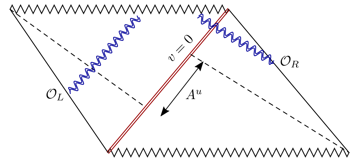
Here, we investigate the effect of backreaction in the opening of the wormhole by applying the double trace deformation in the BTZ geometry perturbed by the shock wave produced by $\phi$. This can be accomplished simply by replacing $U^{\prime}\to U^{\prime}+A^{u}$ in (3.12), which corresponds to apply a shift in the $U$ direction to the bulk-to-boundary propagator that originally connected the left boundary to a point at the horizon. The parameter $A^{u}$ is related to the total momentum sent through the wormhole via

$$A^{u}=-\frac{16\pi G_{N}}{a_{0}\kappa L}p_{v}^{\text{total}}.$$

(4.25)

Alternatively, using the diagnose of traversability of [6], we can apply a translation in the wavefunction $\Psi_{\mathcal{O}_{R}}$

$$\Psi_{\mathcal{O}_{R}}\to e^{-iA^{u}q_{u}}\Psi_{\mathcal{O}_{R}}.$$

(4.26)

For the purpose of the calculation, we can imagine that we send an extra particle with momentum $p_{v}\ll p_{v}^{\text{total}}$. We can then treat this particle as a probe for the opening of the wormhole that will now depend on $p_{v}^{\text{total}}$. In this picture the effective scattering amplitude becomes

$$i\delta_{\text{total}}=-i(A^{u}+a^{u})q_{u}$$

(4.27)

where

$$a^{u}=-\frac{16\pi G_{N}}{a_{0}\kappa L}p_{v}.$$

(4.28)

We can expand in $a^{u}$ to linear order, so that the particle with momentum $p_{v}$ will acquire a shift in the $v$ direction, which we identify as the opening of the wormhole including the backreaction. The integral over $q^{v}$ for the exponent of (4.6) gives

$$\mathcal{D}=\mathcal{D}_{0}\int dt_{1}dx_{1}dx\left(\frac{e^{r_{-}(x-x_{1})}}{\gamma(A^{u}+a^{u})+4e^{-r_{-}(x-x_{1})}\cosh[r_{+}(x-x_{1})]\cosh(\kappa t_{1})}\right)^{2\Delta},$$

(4.29)

where the coefficient $\mathcal{D}_{0}$ is

$$\mathcal{D}_{0}=\frac{hr_{+}^{1+\Delta}\kappa^{2-\Delta}\Gamma(2\Delta)}{\pi\Gamma(\Delta)^{2}}.$$

(4.30)

After expanding to first order in $a^{u}$ we obtain wormhole opening,

$$a^{v}_{\text{back}}=\mathcal{A}_{0}\int\frac{dx\,dt_{1}\,e^{r_{-}(x-x_{1})}}{(4\pi G_{N}e^{r_{-}(x-x_{1})}(-p_{v}^{\text{total}}/L)+\gamma\kappa\cosh(r_{+}(x-x_{1}))\cosh(\kappa t_{1}))^{1+2\Delta}},$$

(4.31)

where $\mathcal{A}_{0}$ is,

$$\mathcal{A}_{0}=-4^{1-2\Delta}hG_{N}\gamma^{2\Delta}r_{+}^{1+\Delta}\kappa^{2+\Delta}\frac{\Gamma(1+2\Delta)}{\Gamma(\Delta)^{2}}.$$

(4.32)