Subband Image Reconstruction using Differential Chromatic Refraction

Modern surveys observe the same region of the sky hundreds or thousands of times over the course of their lifetime. Due to changes in the atmosphere, airmass, and parallactic angle of these observations the image quality and effective throughput of these exposures can vary with time. Time-domain and multicolor studies need to consider these images jointly and, therefore, require advanced methods to combine the data to maximize their information content. Image stacking is one of these techniques and is traditionally accomplished by either coadding images or selecting a small subset of the highest quality data (often referred to as lucky imaging). Coadding can include convolving images to a common resolution before addition [1], combining images within a limited range of image qualities [2], stacking all images while weighting by signal-to-noise [3] or by using a matched-filter approach [4]. Lucky imaging, in contrast, selects the exposures with the highest image quality but at the cost of a reduction in signal-to-noise, and hence depth of the observations. In each of these approaches we sacrifice information (e.g., spatial resolution or depth) for computational expediency or to optimize some aspect about the properties of the images (e.g., image quality).

In Lee et al. [5], we introduced the concept of learning an underlying model that represents the sky from a sequence of images with differing image qualities and depths. In this approach, an image $y_{t}$ at epoch $t$ is a simple convolution of the PSF $f_{t}$ and a latent model image $x$ plus some (uncorrelated) normal noise $\epsilon_{t}$,

$$y_{t}=f_{t}\ast x+\epsilon_{t}\quad\textrm{with}\quad\epsilon_{t,i}\sim{\mathcal{N}}\!\left(0,\sigma_{t,i}^{2}\right)$$

(1)

where $\sigma_{t,i}$ is the estimated standard deviation of pixel $i$, i.e., $\sigma_{t}^{2}$ is the variance map of the $y_{t}$ image. Since the convolution is a linear operation, in the simplified limit of 1-dimensional vectors, the estimated $\hat{y}_{t}$ image can be written as a matrix multiplication

$$\hat{y}_{t}=f_{t}\ast\hat{x}=F_{t}\hat{x}$$

(2)

where $\hat{x}$ is the estimated latent image, without loss of generality. Given a set of $\{y_{t}\}$ exposures and their known $\{f_{t}\}$ PSFs we have shown that we can solve for the model image $x$ in an incremental way by iterating over the observations, considering them one-by-one, and updating the latent model using the data from the current epoch, $t$. Omitting the $t$ index for clarity, the multiplicative update formula is

$$\hat{x}^{\textrm{(new)}}\!=\hat{x}\odot\frac{F^{T}Wy}{F^{T}W\hat{y}}$$

(3)

where the dividing bar and the $\odot$ sign are elementwise division and multiplication operations, and the $\hat{y}\!=\!F\hat{x}$ is the predicted image [6, 5]. The $W$ matrix is a combination of the variance map and the binary masks for the exposure including censored areas, e.g., saturated pixels or bad camera columns, and robust weights that arise as a modified minimization of the dispersion of the $r_{t}=y_{t}-\hat{y}_{t}$ residuals in the form of a function $\rho(t)$ with

$$\min_{\hat{x}}\sum_{t,i}\rho\left(\frac{r_{t,i}}{\sigma_{t,i}}\right)$$

(4)

rather than the traditional

$$\min_{\hat{x}}\frac{1}{2}\sum_{t,i}\left(\frac{r_{t,i}}{\sigma_{t,i}}\right)^{2}$$

(5)

In the classical limit of $\rho(t)\!=\!t^{2}/2$, these two optimization problems are identical, however, for other (more) robust $\rho$-functions, they significantly differ. The typical choice for robust optimization is for $\rho$ to be quadratic for small residuals, but in case of large deviations $\rho$ becomes a constant value, say 1. In this way the contribution of outliers to the cost function is limited [7]. Such robust minimization essentially corresponds to a Maximum Likelihood Estimation using a likelihood function with a longer tail than the Gaussian to accommodate outliers. Our standard solution is an iterative process where we re-weight the quadratic terms with a weight derived from the robust $\rho$-function, $\mathbb{W}(t)\!=\!\rho^{\prime}(t)/t$. In the classical case of $\rho(t)\!=\!t^{2}/2$, the weight is constant 1, but for cases with significant outliers we use a Cauchy distribution with $\mathbb{W}(t)=1/(1+t^{2}/c^{2})$ to down weight these outliers; see Maronna et al. [7], Lee et al. [5].

In this paper, we expand upon these ideas to learn not just the latent image but also to infer the spectral properties of sources from astrometric shifts introduced through differential chromatic refraction (DCR). In Section II we describe our new method capable of extracting color information from sequences of monochromatic images. We apply this technique to simulated images in Section III where we study the limits of the approach in realistic settings. The results and potential applications of this approach are discussed in Section IV.

Astronomical sources emit light across the continuum of the electromagnetic spectrum, $S(\lambda)$, with varying intensity. Observed broadband magnitudes or fluxes $Y$ are an integral over the filter and instrument characteristics $r(\lambda)$ through which the source is observed (including the detector’s quantum efficiency, camera rotator, etc.).

Considering that the CCD counts photons, the equation is given by

$$Y=\frac{\int\!d\lambda\ \lambda\ r(\lambda)\,S(\lambda)}{c\int\!d\lambda\ r(\lambda)/\lambda}$$

(6)

with $c$ is the speed of light. By substituting for a specific filter

$$R(\lambda)=\frac{\lambda\ r(\lambda)}{c\int\!d\lambda\ r(\lambda)/\lambda}\,,$$

(7)

the expression for the flux is significantly simplified,

$$Y=\int\!d\lambda\ R(\lambda)\,S(\lambda)\,.$$

(8)

The above equation applies to each pixel in a $y_{t}$ exposure. The latent image is, however, complicated by the convolution from the PSF and the refraction of the atmosphere. DCR is due to the refraction of light as it passes through the atmosphere similar to light passing through a prism. The differential component of DCR refers to the change in the PSF across the bandpass of a given filter. It results in a positional shift and distortion of a source that depends on the source’s spectral energy distribution [8]. This shift and distortion is a function of wavelength, $f_{t}(\lambda)$, and the altitude and azimuth of the telescope for each epoch, $t$, of the observation. In image coordinates, the effect will also depend on the orientation of the camera rotator. The magnitude of the refraction depends on the temperature and humidity of the atmosphere [9].

Instead of a latent image $x$, we introduce the density image $\xi(\lambda)$, and formulate a more general model as

$$y_{t}=\int\!d\lambda\ R(\lambda)\,\Big[f_{t}(\lambda)\ast\xi(\lambda)\Big]\ +\ \epsilon_{t}$$

(9)

where again the $\ast$ sign denotes the spatial convolution. In the limit of negligible dependence of the PSF on the wavelength, we get back the previous model

$$y_{t}=f_{t}\ast\left[\int\!d\lambda\,R(\lambda)\,\xi(\lambda)\right]\ +\ \epsilon_{t}\ =\ f_{t}\ast x+\epsilon_{t}$$

(10)

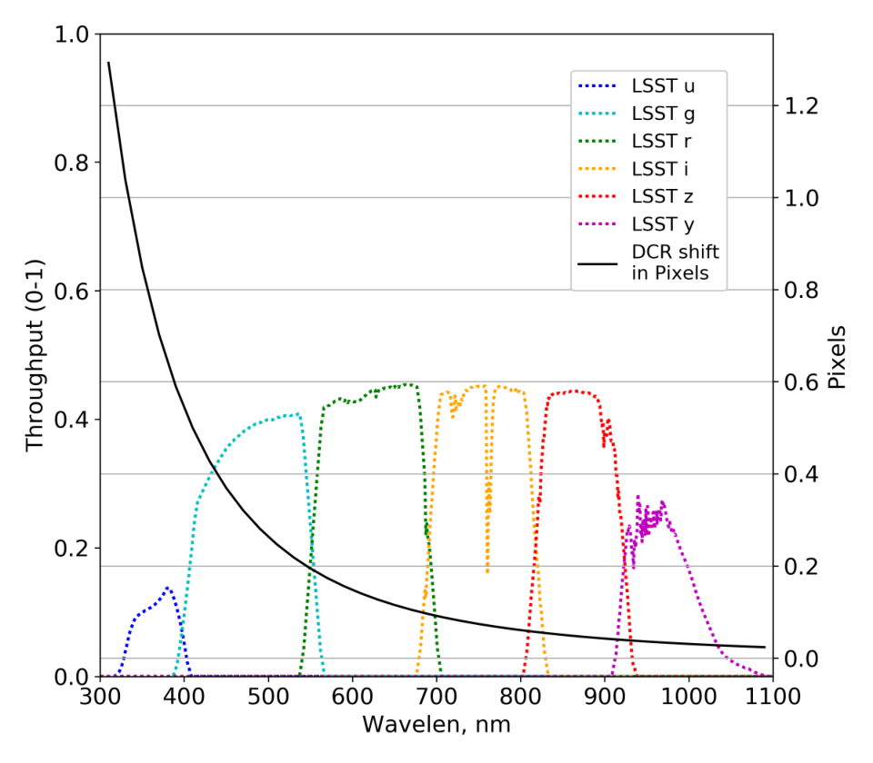
In Figure 1 we illustrate the strength of the astrometric shift as a function of wavelength. The black solid line plotted over the throughput curves shows the relative shift in pixels (0.2 arcsec) for a 10nm difference in observed wavelength. For example the differential shift at a zenith angle of $50^{\circ}$ across the extremes of the u-band, $\lambda_{1}=320\textrm{nm}$ and $\lambda_{2}=400\textrm{nm}$, is over 6 pixels, similarly over the g-band, $\lambda_{1}=400\textrm{nm}$ and $\lambda_{2}=560\textrm{nm}$, it is approximately 5.5 pixels. Of course in reality, the total apparent shift is dependent on the SED of the source [10, 11]. The elongation of the PSF arises because the PSF is simply the weighted summation of all monochromatic PSFs between $\lambda_{1}$ and $\lambda_{2}$.

To account for the wavelength dependence of DCR we, therefore, consider that a latent image is comprised of a number of sub-band images each comprising a limited wavelength interval within a given photometric passband. Given the spectral dependence of the PSF, if we can measure an astrometric offset or variation in the PSF as a function of airmass or parallactic angle (telescope pointing), we can in principle infer the underlying SED. Within these narrower spectral ranges, we assume a constant PSF and SED (though the technique can account for wavelength dependent PSFs even within these sub-bands). We split the filter’s wavelength range $[\Lambda_{0},\Lambda_{K})$ at preset $\{\Lambda_{k}:k\!=\!1\dots{}K\!-\!1\}$ values, and define the response function of these sub-bands as

$$R_{k}(\lambda)=\begin{cases}R(\lambda)&\text{if }\lambda\in[\Lambda_{k-1},\Lambda_{k})\\ \ \ 0&\text{otherwise}\end{cases}$$

(11)

for all $k$ from 1 to $K$. Naturally,

$$y_{t}=\sum_{k=1}^{K}\int\!d\lambda\ R_{k}(\lambda)\,\Big[f_{t}(\lambda)\ast\xi(\lambda)\Big]\ +\ \epsilon_{t}$$

(12)

is equivalent to eq.(9), and its terms can be approximated similarly to that in eq.(10), which yields

$$\hat{y}_{t}=\sum_{k}f_{t,k}\ast\hat{x}_{k}=\sum_{k}F_{t,k}\,\hat{x}_{k}$$

(13)

where each $x_{k}$ is a latent image in the given wavelength range of sub-band $k$, and $F_{t,k}$ is the linear operator that corresponds to the convolution with the PSF $f_{t,k}$ at the appropriate wavelengths.

Introducing a tall $\hat{x}$ vector that contains all these $\hat{x}_{k}$ (1-dimensional) images

$$\hat{x}=\left[\!\!\begin{array}[]{c}\hat{x}_{1}\\ \hat{x}_{2}\\ \vdots\end{array}\!\!\right]\quad\textrm{and}\quad F_{t}=\big[F_{t,1}\ F_{t,2}\ \dots\,\big]$$

(14)

as the horizontal concatenation of the convolution matrices, we can verify that the equation

$$y_{t}=F_{t}\hat{x}+\epsilon_{t}$$

(15)

is equivalent to eq.(13). Considering that eq.(15) is formally the same as the previous model, cf. eqs.(1) and (2), the iterative updates of eq.(3) directly apply to our new wavelength-dependent model.

Furthermore, considering that the transpose of $F$ (omitting the $t$ index) is

$$F^{T}=\left[\!\!\begin{array}[]{c}F_{1}^{T}\\ F_{2}^{T}\\ \vdots\end{array}\!\!\right]\,,$$

(16)

we see that the updates for the individual latent images at different $\lambda_{k}$ wavelengths take the familiar forms of

	$\displaystyle\hat{x}_{1}^{\textrm{(new)}}\!$	$\displaystyle=\hat{x}_{1}\odot\frac{F_{1}^{T}Wy}{F_{1}^{T}W\hat{y}}\ ,$
	$\displaystyle\hat{x}_{2}^{\textrm{(new)}}\!$	$\displaystyle=\hat{x}_{2}\odot\frac{F_{2}^{T}Wy}{F_{2}^{T}W\hat{y}}\ ,$		(17)
		$\displaystyle\,\,\,\vdots$

and so on. The important difference is that now the common $\hat{y}$ term, the predicted image is the sum of the constituents wavelength dependent image,

$$\hat{y}=\sum_{k}F_{k}\hat{x}_{k}\,.$$

(18)

Note that in the limit of a single latent image, we get back the original equations and the corresponding iterative algorithm, hence this is a more general approach With this formalism we can use our robust iterative deconvolution method with only minor modifications. This iterative method is comprised of the following steps. We begin by initializing our models, $\big[\hat{x}_{1}\dots\hat{x}_{k}\big]$, to be uniform in value such that the sum of all pixels is $1.0$, then start by selecting a random observation, $y_{t}$, for which we estimate the appropriate PSF, which we then use in conjunction with equations 17, to update our models. We repeat this procedure until we have reached convergence. Note that we reuse observations, once we have exhausted our unique supply.

To study the properties and limitations of this method we analyze synthetic images with only two components. This essentially corresponds to objects with spectra that only contain two discrete wavelengths. In other words, we attempt to solve for two images at preset wavelengths from a set of exposures that combine these wavelengths into single passband observations.

Deconvolutions such as these are incredibly computationally complex, requiring multiple FFTs per input image for every loop over the set of available image. GPUs or similar massively parallel co-processors are, therefore, required in order to tackle these types workloads within reasonable timeframes. We therefore spent a considerable effort ensuring we optimize the computations our research code to take full advantage of our GPUs. While precise timings vary depending on the available hardware and the runtime settings, most of our our test runs for this article concluded in less than 60 minutes. We make extensive use Nvidia’s cuFFT library as well as a variety of custom CUDA kernels, allowing us to keep the majority of our computation on the GPU while minimizing slow transfers to and from the GPU.

With this work, we show that small extension to our latent image recovery technique [5] enables us to account for the effects of DCR in broadband images and to use the effect of refraction to recover the underlying SED of a source, see also Sullivan [16]. Essentially we can use atmospheric refraction as a low resolution spectrograph to improve the spectral resolution of broadband imaging. Utilizing the LSST filter response curves for the $u$ and $g$ bands (where the DCR effect is strongest) we can improve astrometric and photometric accuracy over standard coaddition techniques that do not incorporate corrections for DCR. From the analysis of the astrometric and photometric performance we show that the improvements in uncertainties in the recovered positions and fluxes are consistent with the increase in signal-to-noise gained by combining multiple images. For intermediate signal-to-noise sources (i.e., SNR$\sim$6) accounting for DCR in the latent image reduces the bias in the astrometric solutions by a factor of five.

While the main focus in this paper has been on resolving two sub-bands, this technique is easily extensible to more sub-bands. In Figure 9, we use our method to resolve 3 subbands given a realistic set of images produced using LSST’s Starfast Simulator [14]. In the left-column we show two example simulated 3-band LSST images where the $g$-band was subdivided into three equally wide wavelength regions. The color dependent position of the sources and the extension of the PSF along the parallactic direction are clearly visible. The simulated observations (where we have a single broadband image) for the $g$-band filter and are shown in the center-column. The DCR induced distortion to the PSF is clearly present within these images. The right panel shows the result of processing 200 $g$-band observations, similar to those in the center-column. This latent image resolves the sub-band images (shown as and inverted RGB) as well as partially deconvolving the underlying image. Considering that the method is able to handle PSFs and pixel sizes of various kinds simultaneously, we expect this method to work across instruments and telescopes as well.

The current model of the latent image of the sky assumes constant brightness across the observations and does not accommodate possible variability of sources explicitly. The robust statistical treatment of our approach will detect the varying flux of these objects and will essentially downweight their observation when they are significantly different from the typical brightness. Variability is a key topic that we plan to address in the future.

A caveat to current study and its conclusions is that the observations of a given astronomical object will not generally have that same distribution as the expected distribution used derived for the whole ensemble. For example, observations of the celestial pole will always occur at the same zenith angle for a given telescope. For a given object (really, a given declination), the zenith angles and parallactic angles available are also highly correlated, occupying a 1-dimensional subspace of the 2d manifold. These effect should be included for detailed analyses for specific experiment.

Our results are consistent with the findings of Sullivan et al.¹¹ 1 LSST report at https://dmtn-037.lsst.io (2018) and demonstrate the potential for such an approach to learn the underlying model for the sky. We note that this first in a series of papers does not include the uncertainties introduced due to PSF estimation and errors in the underlying astrometry. We will address these issues in a forthcoming paper together with the expected spectral resolution that can be achieved by surveys such as the LSST. Given the speed of the GPU implementation we expect that one year of LSST survey data for approximately 50 $\textrm{arcminute}^{2}$ of sky could be processed in less than 30 minutes on a single GPU.

References

- [1] L. Lucy and R. Hook, in Astronomical Data Analysis Software and Systems I, Vol. 25 (1992) p. 277.
- [2] J. Annis, M. Soares-Santos, M. A. Strauss, A. C. Becker, S. Dodelson, X. Fan, J. E. Gunn, J. Hao, Z. Ivezic, S. Jester, et al., arXiv preprint arXiv:1111.6619 (2011).
- [3] A. S. Szalay, A. J. Connolly, and G. P. Szokoly, The Astronomical Journal 117, 68 (1999).
- [4] B. Zackay and E. O. Ofek, The Astrophysical Journal 836, 187 (2017).
- [5] M. Lee, T. Budavari, R. White, and C. Gulian, Astronomy and Computing 21, 15 (2017).
- [6] M. A. Lee and T. Budavári, in Astronomical Data Analysis Software an Systems XXIV (ADASS XXIV), Vol. 495 (2015) p. 261.
- [7] R. Maronna, D. Martin, and V. Yohai, Robust statistics (John Wiley & Sons, Chichester. ISBN, 2006) pp. 34–36.
- [8] J. E. Meyers and P. R. Burchat, The Astrophysical Journal 807, 182 (2015).
- [9] A. V. Filippenko, Publications of the Astronomical Society of the Pacific 94, 715 (1982).
- [10] M. C. Kaczmarczik, G. T. Richards, S. S. Mehta, and D. J. Schlegel, The Astronomical Journal 138, 19 (2009).
- [11] C. M. Peters, G. T. Richards, A. D. Myers, M. A. Strauss, K. B. Schmidt, Ž. Ivezic, N. P. Ross, C. L. MacLeod, and R. Riegel, The Astrophysical Journal 811, 95 (2015).
- [12] J. Sebag and K. Vogiatzis, in SPIE Astronomical Telescopes+ Instrumentation (International Society for Optics and Photonics, 2014) pp. 91500R–91500R.
- [13] B. Rowe, M. Jarvis, R. Mandelbaum, G. M. Bernstein, J. Bosch, M. Simet, J. E. Meyers, T. Kacprzak, R. Nakajima, J. Zuntz, et al., Astronomy and Computing 10, 121 (2015).
- [14] I. Sullivan, “Starfast - a fast simulation building tool for testing algorithms,” (2016).
- [15] S. C. K. C. C. P. S. R. Francisco Delgado, Abhijit Saha, “The lsst operations simulator,” (2014).
- [16] I. Sullivan, “Dmtn-037: Dcr-matched template generation,” (2018).