The Generalized Lasso for Sub-gaussian Measurements with Dithered QuantizationThanks: C. Thrampoulidis and A. S. Rawat are with the Research Laboratory of Electronics, MIT, Cambridge, MA 02139, USA (e-mail: {cthrampo, asrawat}@mit.edu).
Abstract
In the problem of structured signal recovery from high-dimensional linear observations, it is commonly assumed that full-precision measurements are available. Under this assumption, the recovery performance of the popular Generalized Lasso (G-Lasso) is by now well-established. In this paper, we extend these types of results to the practically relevant settings with quantized measurements. We study two extremes of the quantization schemes, namely, uniform and one-bit quantization; the former imposes no limit on the number of quantization bits, while the second only allows for one bit. In the presence of a uniform dithering signal and when measurement vectors are sub-gaussian, we show that the same algorithm (i.e., the G-Lasso) has favorable recovery guarantees for both uniform and one-bit quantization schemes. Our theoretical results, shed light on the appropriate choice of the range of values of the dithering signal and accurately capture the error dependence on the problem parameters. For example, our error analysis shows that the G-Lasso with one-bit uniformly dithered measurements leads to only a logarithmic rate loss compared to the full-precision measurements.
I Introduction
I-A Motivation
Over the last decade or so, the problem of structured signal recovery from high-dimensional linear measurements has received considerable attention. In its most classical formulation the problem asks to recover a signal from (noisy) linear measurements , , where , are the measurement vectors and represents a noise component. In the high-dimensional setting of interest both the dimension of the signal’s ambient space , as well as the number of measurements are large. Moreover, there is typically some prior structural knowledge about the unknown signal , which manifests itself in many forms such as sparsity, low-rankness, sparse derivatives, etc.
While many recovery algorithms have been proposed and analyzed in the literature, perhaps the most popular one is the Generalized Lasso (G-Lasso), which minimizes a least-squares objective function subject to a regularization constraint that promotes the prior structural knowledge on (e.g., -norm for sparse recovery and nuclear norm for low-rank matrix recovery). In its general form the G-Lasso obtains an estimate by solving the following (convex) optimization program for some appropriate (convex) constraint set 11 1 The discussion that follows, as well as, all the results presented in this paper do not require the set to be convex. However, convex constraint sets make (1) a convex optimization program; thus, they are often preferred in practice for computational purposes..
| (1) |
By now, there is a very good understanding of the algorithm’s recovery performance; the guarantees apply for general types of structure (and the corresponding constraint sets ) and hold under wide range of assumptions on the measurement vectors. It is rather typical that the analysis is performed under the assumption that the measurement vectors are realized from some probability distribution. For example, suppose that the measurements are centered sub-gaussian and that the noise is sub-gaussian and independent of the measurements, with entries iid of variance . Then, with high-probability, it holds22 2 Throughout the introduction, we are being deliberately informal in order to streamline the presentation and focus on the main points: the symbol hides positive constants and “high-probability” is not quantified. We refer the reader to the remaining sections of the paper for formal statements., [CRPW12, Tro15]:
| (2) |
provided that . In (2) the quantity is a geometric summary parameter, called the Gaussian width, which captures the geometry of the set with respect to the particular . While deferring its formal definition to Section II, it is important for our discussion to remark the following. First, despite being an abstract parameter, it is often possible to compute sufficiently accurate approximations that reveal the explicit role of primitive problem parameters. For example, for an -sparse and being a scaled -ball, it can be shown that . Second, the result stated above not only captures the correct error rate decay, but also, it captures the minimum required number of measurements to guarantee this decay, i.e., .
However, in many practical settings, full-precision measurements that have been assumed thus far in this discussion are not available. Instead, one observes quantized linear measurements , where is the quantization scheme at hand. For example, consider the following two commonly encountered quantization schemes (cf. Figure 1).
- •
Uniform (mid-riser) quantization: For some level , 33 3 For , denotes the largest integer that is smaller than .
- •
One-bit quantization:
This gives rise to the following natural question:
How to recover a structured signal from high-dimensional measurements ? Moreover, can we obtain recovery guarantees that resemble (2)?
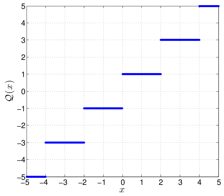
Uniform quantization with .
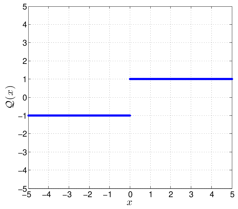
One-bit quantization.
First of all, notice that the task above is naturally harder than recovery from full-precision linear measurements, as the quantized measurements are clearly less informative. A simple illustrative example is to assume that and the noiseless setting (). Then, for the full-precision measurements, under mild assumptions, it is easy to perfectly recover by just inverting the system of linear equations. On the other hand, recovery becomes challenging when only one-bit measurements are available; even, in the absence of noise we may not hope to perfectly recover . Onwards, we focus only on the noiseless setting since it is already challenging for quantized measurements and it also leads to easier exposition.
Perhaps surprisingly, Plan and Versyynin [PV16] demonstrated that, even with quantized measurements, the G-Lasso achieves good recovery performance when the measurement vectors are Gaussian44 4 The question of structured signal recovery from quantized measurements (specifically, one-bit measurements) has been subject of numerous works over the past decade. We postpone a reference on this line of research to Section I-D, and instead, we focus on the directly relevant work [PV16].. An appealing feature of their theoretical result is that, similar to (2), their error bounds are simple to state and clearly isolate the effect of the specific quantization scheme, on one hand, and of the problem geometry, on the other hand. To be more concrete the authors [PV16] show that, with high probability, the estimator
| (3) |
satisfies
| (4) |
provided that . In this expression, the non-zero parameters and depend on the specific quantization function . For example, it can be shown that , for one-bit measurements, and, , for uniformly quantized measurements. For simplicity, we drop the subscript when the specific scheme in reference is clear from context. We now make the following two crucial remarks regarding (4).
- •
- •
Gaussian measurements: The validity of (4) requires that the measurement vectors are Gausssian.
In this work, we address both of the aforementioned weaknesses. We show that in the presence of appropriate dithering in the quantization scheme, the same algorithm (3) can recover not only direction but also norm information for distributions of the measurement vectors beyond Gaussians. Our results apply to both of the quantization schemes mentioned above, and they also inherit many of the interpretability features of (2) and (4).
I-B Contribution
We consider quantized linear measurements with appropriate dithering. Dither is a purposeful applied random noise component that is added to an input signal prior to its quantization. This technique is rather well-established and commonly used both in practice (because it can result in more subjectively pleasing reconstructions) and in theory (because it often results in favorable statistical properties of the quantization noise); e.g., see [GS93, DK06] and references therein. More recently, dithered quantization has been also exploited and studied in the context of high-dimensional structured signal recovery from quantized linear measurements [BFN+17, KSW16, XJ18, DM18]. Our work builds upon such recent results, in particular [XJ18, DM18]; see Section I-D for a detailed discussion.
In a nutshell, we show that the G-Lasso can be used to efficiently recover structured signals from (appropriately) dithered quantized linear measurements. More precisely, we study the recovery method in (3) for appropriate value of the parameter when the measurements are of the form , where is the dithering signal and is either the uniform or the one-bit quantizer. We consider sub-gaussian measurement vectors of sub-gaussian norm at most (see Section II).
Out results are rather easy to state. We include here an informal version to allow direct comparisons to (2) and (4). Formal statements and detailed discussions follow in later sections.
Uniform dithered quantization
For , let the measurements be given as follows:
| (5) |
where and . We solve the G-Lasso in (3) setting and we show that,
| (6) |
provided that . Note the resemblance of this result to (2). We may conclude that essentially the G-Lasso treats the quantization error (up to an absolute constant) as an independent noise component of strength 55 5 It is rather straightforward to see that the quantization error is a random variable that is absolutely bounded by under the quantization scheme in (6). On the other hand, this random variable is not independent of the measurements. Thus, (2) is not applicable and showing that (6) holds requires additional effort. Also, observe that unlike (4) our guarantee does not require knowledge of the norm of the signal .
One-bit dithered quantization.
For , let the measurements be given as follows:
| (7) |
where and . Furthermore, assume a known upper bound on the true norm of signal , i.e., known such that . Our main result suggests setting for some absolute constant and solving (3) while setting . Then, we show that
| (8) |
provided that . Here, Observe that despite only having one-bit information, the proposed estimator leads to only a logarithmic loss with respect to the best possible error rate in (2).
In the coming sections we also discuss (possible) extensions of this theory to other dithering distributions and to other random measurement models. We also corroborate our theoretical findings with numerical simulations.
I-C Proof sketch
A simple key inequality
We start by denoting the loss function in (3) as
Let be a solution of (3) and denote the error vector. If there is nothing to prove and so we assume onwards that this is the case. By optimality of (consequently, of ), we have that
| (9) |
where the equality holds by simple algebraic manipulations. Rearranging that expression yields
which is our starting point to obtain an upper bound on . Recall that , which leads to , where denotes the cone of descent directions or tangent cone (cf. Definition II.1). Therefore, we can deduce the following key fact:
| (10) |
where denotes the unit sphere in . The rest of the proof amounts to lower (upper) bounding the of the involved random processes in (10). Applying those bounds in (10) naturally leads to the results stated in (6) and (8).
Lower bound.
Upper bound
We will show how to upper bound in (10), where the expectation is over all the involved random variables, i.e., the ’s and ’s. This leads to a constant probability bound (say with probability at least ) by Markov inequality, but more powerful techniques can also be applied to yield similar bounds that hold up to probability of failure that goes to zero with increasing number of measurements. For the ease of exposition, we denote the quantization noise as follows:
| (11) |
In the sequel, keep in mind that is not independent of the measurement vectors . Also, for a random process indexed by , let us denote
| (12) |
By observing that , it easily follows that
| (13) |
where, for each , and are iid copies of and , respectively. Now, we need to show that both Term I and Term II are small. We may think of these as a bias (Term II) and variance (Term I) terms. Appropriately selecting the dithering signal helps reduce the bias in the estimate. At the same time, since the dither signal is not known, it acts as a source of noise and naturally increases the variance of the estimate.
Here, in oder to keep this proof sketch short, we focus on Term II. This alone already demonstrates the value of dithering and guides the correct choice of the parameter . The details regarding bounding Term I can be found in later sections. We consider Term II separately for each one of the quantization schemes that we wish to analyze.
Uniform quantization. The key observation here is that for all inputs the quantization noise of a uniform quantizer with uniform dithering (see (5)) is a mean zero random variable, i.e.,
| (14) |
This is a classical fact in the theory of dithered quantization (see Section III for a discussion) [GS93]. By using this fact and the tower property of expectation, one easily finds that Term II is equal to zero:
| (15) |
One-bit quantization. As compared to the uniform quantization, the quantization noise in the case of -bit quantization is not zero-mean. However, with an appropriate choice of we can still make Term II small enough. A simple calculation yields the following for the quantization scheme in (7):
Hence, by choosing , we have that
| (16) |
In (13) the role of above is played by . Clearly the right-hand side in (16) is non-zero for general values of , but we can hope of making it small by choosing large enough so that the events under which the indicator functions become active are rare. To see this, recall our assumption that is isotropic -subgaussian, from which it follows that Notice that this probability can be made sufficiently small by setting . Of course, a little more work is needed to translate this into being small, but at this point we defer the rest of the details to later sections (see Lemma B.1).
Remark 1 (Literature).
The method for analyzing the G-Lasso performance based on (10) has been commonly used in several recent works. In fact, this is the starting point not only for the analysis under dithered quantized measurement, but also for the error bounds in (2) and (4), e.g. [PV16]. Beyond that, as previously mentioned, the lower bound is based on Mendelson’s small-ball method [Men15, KM15]. For the upper bound: (Term I) we carefully put together several known techniques in the study of suprema of random processes (such as symmetrization, Rademacher contraction principle, majorizing measure theorem, etc.; see Lemmas A.2 and B.2); (Term II) we exploit the fact that dithering causes the quantization noise to behave in a statistically nice fashion. Although this latter idea is well-known, in the context of our paper, it was brought to our attention by the recent works [DM18, XJ18]. More precisely: (i) Identity (14) is the key fact used in [XJ18] (but also, see earlier classical works on dithered quantization, e.g., [GS93]); (ii) Identity (16) is previously derived and exploited in the same way in [DM18] (but also, see earlier work [DK06])
I-D Related Work
Our work naturally fits in the recent developments in the study of structured signal recovery from high-dimensional random measurements. With the advent of Compressive Sensing (CS), there has been a very long list of papers that collectively have significantly advanced our understanding regarding the performance of convex-optimization based methods in the case of (full-precision) noisy linear measurements. Perhaps the most widely used and most well-studied among such methods is the Generalized Lasso in (1) (and its variants). By now, there exists a rich, elegant and general theory that accurately (only up to absolute constants) characterizes the recovery performance of the G-Lasso under quite general assumptions on the measurements vectors (iid Gaussians, sub-gaussians, sub-exponentials, etc.), e.g., see [RV06, Sto09, DMM11, CRPW12, ALMT14, Sto13, OTH13, Tro15, SBR15, OT15]. In this paper, we extend this line of work by establishing recovery guarantees for the G-Lasso in the practical settings with quantized measurements. The error bounds that we derive are reminiscent of the existing results in the case of the full-precision measurements.
Structured signal recovery from quantized high-dimensional measurements has also been extensively studied in the literature. The vast majority of the related works focuses on the case of one-bit quantization (often termed 1-bit CS) without dithering, for which case norm recovery is impossible, e.g., see [BB08, PV13, JLBB13]. Also, most of these works, only apply to iid Gaussian measurements, with a few exceptions such as [ALPV14]. On the other hand, it was recently demonstrated that dithering has the advantage of making norm-recovery possible: [KSW16] considers iid Gaussian dithering signal, while [BFN+17] studies an adaptive dithering scheme. Both of these works are limited to iid Gaussian measurements and sparse signal recovery. It has only been very recent work due to Xu and Jacques [XJ18], who (to the best of our knowledge) first demonstrated that a uniform quantization scheme combined with a uniformly distributed dithering signal promises pushing much of the theory beyond Gaussian measurements. Shortly afterwards, Dirksen and Mendelson [DM18] extended this idea to one-bit measurements with appropriate uniform dithering. These two papers have motivated our work. We show that a single recovery algorithm can successfully be used for both quantization schemes considered in [XJ18] and [DM18]. Importantly, this algorithm is the well-established G-Lasso algorithm with a single tuning parameter , which changes depending on the specifics of the quantization scheme. In terms of theory, our analysis yields easily interpretable results that nicely fit in the existing literature on the full-precision measurements. Practically, the potential advantage of using the G-Lasso is that one can rely on the abundance of efficient specialized solvers for this program. We empirically observe that the G-Lasso significantly outperforms the simple recovery scheme proposed in [XJ18] for uniform quantization. On the other hand, the G-Lasso appears to perform similarly to the algorithm proposed in [DM18]. Yet, the former has the advantage of being directly applicable to uniformly quantized measurements. Also, our analysis suggests explicit guidelines on the choice of the threshold , which controls the range of dithering (7), and of the tuning parameter in (3).
Finally, our paper is very closely related to the work of Plan and Vershynin [PV16], who studied the G-Lasso for non-linear observations, which includes quantization as a special case. Unfortunately, their results do not guarantee norm-recovery and are limited to Gaussian measurements. Our work removes these limitations in the case of quantized measurements.
I-E Organization
The rest of the paper is organized as follows. In Section II, we introduce various key geometric quantities that are relevant to our analysis and state the underlying assumptions on the measurement vectors. We present our main results and accompanying discussions for the uniform dithered quantization and the one-bit dithered quantization models in Section III and Section IV, respectively. In Section V, we evaluate the recovery performance of (3) using synthetic experiments and compare it with the existing methods in the literature. We conclude the paper by highlighting multiple concrete directions for future work in Section VI. We have relegated all the proof to appendices to enhance the readability of the paper.
II Background
II-A Geometric notions
First, we introduce the notions of the tangent cone and the Gaussian width.
Definition II.1 (Tangent cone).
The tangent cone of a set at is defined as
Definition II.2 (Gaussian width).
The Gaussian width of a set is defined as
| (17) |
The Gaussian width plays a central role in asymptotic convex geometry. In particular, its square can be formally described as a measure of the effective dimension of the set [Ver17, ALMT14]. More recently, the Gaussian width has played a key role in the study of linear inverse problems. This is already revealed in (2) which requires that the number of measurements be larger than (a constant multiple of) the squared Gaussian width of a spherical section of the corresponding descent cone [Sto09, CRPW12, Tro15].
II-B Sub-gaussian vectors
Throughout this paper, we work with sub-gaussian measurement vectors. For the reader’s convenience, we recall the definition of sub-gaussian vector below; see e.g., [Ver17, Ch. 2] for an introduction to sub-gaussian random variables.
Definition II.3 (Sub-gaussian vectors).
A random vector is called sub-gaussian with sub-gaussian norm if the one-dimensional marginals are sub-gaussian random variables for all and
where we recall that the sub-gaussian norm of a random variable is defined as follows
Specifically, we make the following assumption on the measurement vectors .
Assumption 1 (Sub-gaussian measurements).
We assume that each vector is an iid copy of a random vector that satisfies the following properties.
- •
Subgaussian marginals: is a sub-gaussian random vector with .
- •
Symmetry: has a symmetric distribution. In particular this implies .
- •
Nondegeneracy: There exists such that for each , we have .
III Uniform quantization
In this section we study the problem of exact signal recovery from the observations generated by the uniform dithered quantization. In particular, we aim to recover a signal of interest from measurements given by (5). Our estimate of solves (3) with parameter . We assume that the measurement vectors satisfy Assumption 1. Our main result is as follows; we defer its proof to Appendix A.
Theorem III.1.
[Error analysis: uniform dithered quantization] Suppose that the vectors satisfy Assumption 1. For a fixed vector , let the measurements be given as in (5) and let be a solution to (3) with parameter . Finally, for the constraint set in (3), define the shorthand . Then, there exist positive constants such that the following holds with probability at least 0.99:
provided that
| (18) |
III-A Remarks and Extensions
On the constant probability bound
As stated, the error bound of the theorem holds with constant success probability. However, it is possible to extend the result to hold with success probability that goes to one as the dimension of the problem increases. This requires applying a few technical results on concentration properties of the suprema of random processes (e.g., [D+15]). Since this does not contribute to the essence of our results, we have decided to keep the exposition simple by focusing only on the constant probability bounds (similar to [PV16]).
Limit of full-resolution measurements
In the limit of the resolution of the quantizer , the quantized measurements in (5) approach the (noiseless) full-resolution measurements In that limit, Theorem III.1 suggests that provided that . As expected, this conclusion is in full-agreement with the well-established results on the phase-transition of noiseless linear inverse problems with full-resolution measurements, e.g., [Tro15].
On the distribution of the dithering signal
As previously mentioned, dithering is essential for the validity of the theorem. This is also revealed in the proof, where the specific uniformly distributed dithering signal guarantees that the quantization noise has zero mean conditioned on the input signal (cf. (15)). This raises a natural question: what are other dithering distributions (other than uniform) that guarantee that (15) holds. This question is well-studied in the literature of dithered quantization; in fact, the entire class of such distributions is characterized and we refer the interested reader to the excellent exposition in [GS93, Thm. 2] for details. As an example, (15) also holds when are iid and distributed as the sum of uniform random variables in . To further relate this classical result to Theorem III.1, note that the theorem essentially remains valid for all such distributions for the dither signal with bounded support.
Examples
The results of Theorem III.1 apply under rather general assumptions on and on the choice of the constraint set . Here, for mere illustration, we provide two concrete examples for the most popular instances of structured signal recovery problems.
- •
- •
Low-rand recovery: Assume that , where has rank . We further choose
where denotes the nuclear norm. In this case, it is well-known (e.g., [CRPW12]) that
(20) Thus,
provided that
Boundary of
In the examples provided above, the set is chosen such that lies on its boundary. This condition is, in general, a prerequisite so that the cone of descent directions is not the entire space and that the upper bound of Theorem III.1 in terms of is especially useful. Otherwise, and , in which case the error bound fails to capture the role of and of the structure of . When is a star-shaped set (in particular, this holds when is convex), then it is possible to break that limitation of Theorem III.1 by only slightly modifying the proof and by introducing the “local Gaussian width” in place of the Gaussian width considered here. The technical arguments towards these modifications are well-explained in [PV16, Thm. 1.9]. The focus of Theorem III.1 (also, of Theorem IV.1) is on capturing the role of dithered quantized measurements on the recovery performance of the G-Lasso. Hence, we refer the reader to the related works [PV16] for extensions regarding capturing the role of and of .
Sub-exponential measurements
It is possible to extend the result of Theorem III.1 (with appropriate modifications on the error bound) to a wider class of measurement vectors, in particular to sub-exponential distributions. Indeed, a close inspection of the proof of Theorem III.1 reveals that the fact that measurement vectors follow a sub-gaussian distribution is essentially only critical in lower bounding the left-hand side of (10) and in upper bounding the empirical width (see Appendix A-C). Since corresponding lower and upper bounds are also available for sub-exponential measurement vectors [Tro15, Oym18], it is possible to extend Theorem III.1 in that direction.
Related results
Essentially, Theorem III.1 can be viewed as an extension of the corresponding results in [PV16] (which are only true for Gaussians measurements) to sub-gaussian measurements66 6 Of course, Plan and Vershynin [PV16] study the generalized linear measurement model to which the quantized measurement model is only a special case. Note that the authors state their result under the additional assumption that (see (4)). However, in the case of uniform dithered quantization with uniformly distributed dither signal, it is relatively easy to extend their result by waiving the assumption. We omit the details for brevity.. Xu and Jacques [XJ18] were the first to study the effect of dithering in uniform quantization schemes in the high-dimensional setting. To showcase the favorable properties of dithering they analyzed the performance of a simple projected back projection (PBP) method. Naturally, as also confirmed via simulations in Section V, our proposed algorithm in (3) outperforms PBP method. On the other hand, using a different type of analysis, Xu and Jacques are able to extend their result to wider classes of measurement distributions beyond sub-gaussians.
On the number of quantization bits
The uniform quantization scheme studied thus far does not assume any constraints on the number of bits used for quantization of the input signal . In general, the input signal can take very large values (relative to the resolution value ) and thus it may require a large number of quantization bits, which might be impractical. A possible solution to this issue is to perform clipping, that is to limit the number of quantization levels to some fixed value . Unfortunately, clipping introduces an additional source of error to the measurement model (often referred to as overload distortion). Hence, it is not obvious at the outset how this affects the error bound of Theorem III.1. In the next section, we study one-bit quantization, which can be viewed as an extreme case of clipping (). Extending these results to the quantizers with general values of is an interesting direction for future research.
IV One-bit quanitzation
We explore the problem of exact signal recovery from one-bit dithered observations when the measurement vectors are sub-gaussian. Recall that we are working with the measurements of a signal of interest given by (7). The dithered signal is uniform in , and our main result specifies appropriate values for the range parameter . Our estimate of solves (3) with parameter .
We present the main result of this section in Theorem IV.1 below. All the proofs are deferred to Appendix B.
Theorem IV.1.
[Error analysis: one-bit dithered quantization] Suppose that the vectors , satisfy Assumption 1. Fix any and let be such that . Assume that the measurements are given as in (7) with range parameter and let be a solution to (3) with parameter . Finally, for the constraint set in (3) define the shorthand . Then, there exist positive constants such that the following holds with probability at least 0.99:
provided that and
IV-A Remarks
On the error decay with
Theorem IV.1 guarantees an error decay as a function of the number of measurements. Therefore, an important conclusion of the theorem is that the proposed LASSO estimator in (3) only leads to loss with respect to the best possible rate (see (2)). In other words, despite only having (appropriately dithered) one-bit measurements there is relatively little loss in performance with respect to full precision samples.
Gaussian measurements
When the measurement vectors have entries iid Gaussian, it is possible to perform a tighter analysis, which is presented in Appendix B-C and which leads to the following result.
Theorem IV.2 (Gaussian measurements).
Let the same setting as in Theorem IV.1 except that the measurement vectors , are assumed to have iid standard normal entries. Then, for sufficiently large , there exist absolute constants such that the following holds with probability at least 0.99:
provided that and
Compared to Theorem IV.1, the theorem above specifies the quantization parameter with an exact constant for Gaussian measurements. In our simulations, we observe that the same value yields good results even for other sub-gaussian distributions. Also, observe the close agreement in the error formulas of the two theorems. The formula in Theorem IV.1 has an extra factor; however, note that this term disappears in the overdetermined regime . Finally, in the Appendix B-C we obtain an even tighter expression for the error bound than the one that appears above. It is also shown that the former simplifies to the latter at the cost of requiring that is large enough and an extra multiplicative constant (that can be shown to approach 2 for increasing ).
On the classical statistics regime
The pervasive working assumption in classical statistics is that the number of measurements grows large , while the signal dimension remains fixed. In that context, signal recovery from dithered one-bit measurements using least-squares (i.e., (3) without any constraints) was previously studied by Dabeer and Karnik [DK06, Thm. 1]. Compared to their result, Theorem IV.2 is valid more generally: (i) it is non-asymptotic; (ii) it applies to the the high-dimensional regime (both and large); (iii) it captures the role of the constraint set . As expected, when specialized to the classical statistics regime, our theorem is in full agreement with [DK06, Thm. 1], which also captures the -rate.
On the dithering distribution
Theorem IV.1 assumes iid uniform dithering signals in the interval , as well as a specific choice of . A first interesting question is what is the best possible rate as a function of for uniform dithering signals: is it possible to improve upon the logarithmic rate loss of Theorem IV.1? A second question asks whether better rates can be obtained with different distributions for the dithering signal. Interestingly, Dabeer and Karnik [DK06, Thm. 2] give a negative answer to the latter question in the classical asymptotic regime with large and fixed . It is interesting to study these questions in the high-dimensional regime that is of modern interest.
On the scaling with
Note that the proposed scheme requires knowledge of an upper bound on the true norm of the unknown signal. Indeed, both the quantization-scheme parameter and the G-Lasso parameter are required by Theorem IV.1 to be proportional to such a value . Moreover, the theorem predicts that the normalized estimation error scales linearly with the the overshoot in our guess regarding the signal’s norm.
Examples
Related results
As mentioned before, our work is in-part motivated by recent results in [DM18]. In the context of uniformly dithered one-bit quantization, Dirksen and Mendelson [DM18] propose and analyze a different convex-optimization based estimator which shares some similarity with the LASSO in (3). Specifically, put in our notation, they solve the following program
| (21) |
where the value of the regularizer is set to . To see that this is indeed rather similar to the G-Lasso objective in (3), expand the squares in the latter and recall that we set . Empirically, we have observed that the two algorithms perform similarly for iid sub-gaussian measurements, when the value of is set according to our Theorem III.1. However, note that the G-LASSO also works for the uniform quantization scheme with only a simple tuning of the parameter . In terms of theoretical results, the error guarantees of Theorem III.1 and our suggested value for are not directly comparable to corresponding results in [DM18, Thm. 1.3], which are (perhaps) less explicit in terms of the problem parameters, e.g., , , , etc.. For example, our result naturally suggests a “good” value of . On the other hand, we mention that [DM18, Thm. 1.3] holds under a more general setting since it also accounts for pre- and post-quantization noise and also yields uniform guarantees over all . We leave such extensions of our results as future work.
V Simulations
In this section we experimentally evaluate the recovery performance of the Generalized LASSO in (3) when dithered quantized measurements are available. We consider both the uniform and the one-bit quantization schemes in the presence of uniformly distributed dithering, as shown in (5) and (7), respectively. In addition, we compare the performance of the method with corresponding ones proposed recently in [XJ18] and [DM18] for uniform and one-bit quantization, respectively.
We present results in which the measurements vectors have entries that are iid Rademacher random variables77 7 A Rademacher random variable takes two valued with equal probability.. Throughout our experiments, we keep the dimension of the signal fixed . The unknown signal is chosen to be -sparse constructed as follows. First, we select the support of uniformly at random among all possible supports. Then, the non-zero entries of are sampled iid from the standard normal distribution. Finally, we scale the entries of the signal such that . For one-bit measurements, we choose . In order to estimate , we solve the G-Lasso in (3) with using the CVX package for Matlab [GBGB]. The parameter in (3) is set to for uniform quantization and to for one-bit measurements. Throughout this section, each plot is obtained by averaging over Monte Carlo realizations, with independently sampled measurement vectors , signal vector , and dithering across different trials.


In Figure 2, we compare the G-Lasso (cf., (3)) with the projected back projection (PBP) method from [XJ18] for the case of uniform dithered quantization. Observe that the error plots for (3) concur with the scaling as predicted by Theorem III.1. Furthermore, note that (3) significantly outperforms the PBP method. Another advantage of (3) is its dependence on the parameter : when continuously decreasing the value of (which results into more informative measurements), this leads to sustained decrease in the recovery error (cf., Remark III-A). On the other hand, the PBP hits an error floor as the measurements increase, thus failing to utilize the information present in the measurements beyond a certain point. This phenomenon is clearly illustrated in Figure 3.
Focusing on the one-bit dithered quantization scheme (cf. (7)), we plot the recovery performance of the G-Lasso in Figure 4. Note that the recovery performance demonstrates a scaling that behaves as with increasing , as suggested by Theorem IV.2. During our experiments, we also observed that the performance of the G-Lasso is almost identical to that the alternative algorithm in (21) from [DM18]. However, as discussed in Section IV-A, our method offers additional benefits such as: (i) An explicit choice of the parameters appearing in the objective function. (Note the is associate with the parameter , which controls the range of the dithering.) (ii) An algorithm that is already well-established and can be commonly used both for one-bit, as well as, uniform quantization schemes.
VI Future work
There are several directions for future work related to the results presented in this paper. Some of the straightforward ones, include extensions to account for pre- and post-quantization noise, as well as, establishing uniform guarantees over all unknown signals of interest. Also, in Section IV we discussed a number of questions regarding other distributions for the dithering signal, the potential optimality of the error rate of in Theorem IV.1, etc.
One can also imagine extending our results to general quantization schemes, e.g, general number of quantization levels [TAH15]. Finally, considering other loss functions in (3) (e.g., see [Gen17]) and the performance of first-order solvers (e.g., see [OS16]) are also interesting directions to pursue.
References
- [ALMT14] Dennis Amelunxen, Martin Lotz, Michael B. Mccoy, and Joel A. Tropp. Living on the edge: Phase transitions in convex programs with random data. Information and Inference, 3(3):224–294, Sep. 2014.
- [ALPV14] Albert Ai, Alex Lapanowski, Yaniv Plan, and Roman Vershynin. One-bit compressed sensing with non-gaussian measurements. Linear Algebra and its Applications, 441:222–239, 2014.
- [BB08] Petros T Boufounos and Richard G Baraniuk. 1-bit compressive sensing. In 2008 42nd Annual Conference on Information Sciences and Systems (CISS), pages 16–21. IEEE, 2008.
- [BFN+17] Richard G Baraniuk, Simon Foucart, Deanna Needell, Yaniv Plan, and Mary Wootters. Exponential decay of reconstruction error from binary measurements of sparse signals. IEEE Transactions on Information Theory, 63(6):3368–3385, 2017.
- [CRPW12] Venkat Chandrasekaran, Benjamin Recht, Pablo A Parrilo, and Alan S Willsky. The convex geometry of linear inverse problems. Foundations of Computational Mathematics, 12(6):805–849, 2012.
- [D+15] Sjoerd Dirksen et al. Tail bounds via generic chaining. Electronic Journal of Probability, 20, 2015.
- [DK06] Onkar Dabeer and Aditya Karnik. Signal parameter estimation using 1-bit dithered quantization. IEEE Transactions on Information Theory, 52(12):5389–5405, 2006.
- [DM18] Sjoerd Dirksen and Shahar Mendelson. Robust one-bit compressed sensing with non-gaussian measurements. arXiv preprint arXiv:1805.09409, 2018.
- [DMM11] David L Donoho, Arian Maleki, and Andrea Montanari. The noise-sensitivity phase transition in compressed sensing. Information Theory, IEEE Transactions on, 57(10):6920–6941, 2011.
- [GBGB] Michael Grant, Stephen Boyd, Michael Grant, and Stephen Boyd. Cvx: Matlab software for disciplined convex programming, version 2.1. Recent Advances in Learning and Control, pages 95–110.
- [Gen17] Martin Genzel. High-dimensional estimation of structured signals from non-linear observations with general convex loss functions. IEEE Transactions on Information Theory, 63(3):1601–1619, 2017.
- [Gor88] Yehoram Gordon. On milman’s inequality and random subspaces which escape through a mesh in . 1988.
- [GS93] Robert M Gray and Thomas G Stockham. Dithered quantizers. IEEE Transactions on Information Theory, 39(3):805–812, 1993.
- [JLBB13] Laurent Jacques, Jason N Laska, Petros T Boufounos, and Richard G Baraniuk. Robust 1-bit compressive sensing via binary stable embeddings of sparse vectors. IEEE Transactions on Information Theory, 59(4):2082–2102, 2013.
- [KM15] Vladimir Koltchinskii and Shahar Mendelson. Bounding the smallest singular value of a random matrix without concentration. International Mathematics Research Notices, 2015(23):12991–13008, 2015.
- [KSW16] Karin Knudson, Rayan Saab, and Rachel Ward. One-bit compressive sensing with norm estimation. IEEE Trans. Information Theory, 62(5):2748–2758, 2016.
- [LT91] Michel Ledoux and Michel Talagrand. Probability in Banach Spaces: isoperimetry and processes, volume 23. Springer, 1991.
- [Men15] Shahar Mendelson. Learning without concentration. Journal of the ACM (JACM), 62(3):21, 2015.
- [OS16] Samet Oymak and Mahdi Soltanolkotabi. Fast and reliable parameter estimation from nonlinear observations. arXiv preprint arXiv:1610.07108, 2016.
- [OT15] Samet Oymak and Joel A Tropp. Universality laws for randomized dimension reduction, with applications. arXiv preprint arXiv:1511.09433, 2015.
- [OTH13] Samet Oymak, Christos Thrampoulidis, and Babak Hassibi. The squared-error of generalized lasso: A precise analysis. arXiv preprint arXiv:1311.0830, 2013.
- [Oym18] Samet Oymak. Learning compact neural networks with regularization. arXiv preprint arXiv:1802.01223, 2018.
- [PV13] Yaniv Plan and Roman Vershynin. One-bit compressed sensing by linear programming. Communications on Pure and Applied Mathematics, 66(8):1275–1297, 2013.
- [PV16] Yaniv Plan and Roman Vershynin. The generalized lasso with non-linear observations. IEEE Transactions on information theory, 62(3):1528–1537, 2016.
- [RV06] Mark Rudelson and Roman Vershynin. Sparse reconstruction by convex relaxation: Fourier and gaussian measurements. In Information Sciences and Systems, 2006 40th Annual Conference on, pages 207–212. IEEE, 2006.
- [SBR15] Vidyashankar Sivakumar, Arindam Banerjee, and Pradeep K Ravikumar. Beyond sub-gaussian measurements: High-dimensional structured estimation with sub-exponential designs. In Advances in neural information processing systems, pages 2206–2214, 2015.
- [Sto09] Mihailo Stojnic. Various thresholds for -optimization in compressed sensing. arXiv preprint arXiv:0907.3666, 2009.
- [Sto13] Mihailo Stojnic. A framework to characterize performance of lasso algorithms. arXiv preprint arXiv:1303.7291, 2013.
- [TAH15] Christos Thrampoulidis, Ehsan Abbasi, and Babak Hassibi. LASSO with non-linear measurements is equivalent to one with linear measurements. In Advances in Neural Information Processing Systems, pages 3420–3428, 2015.
- [Tal06] Michel Talagrand. The generic chaining: upper and lower bounds of stochastic processes. Springer Science & Business Media, 2006.
- [Tro15] Joel A Tropp. Convex recovery of a structured signal from independent random linear measurements. In Sampling Theory, a Renaissance, pages 67–101. Springer, 2015.
- [Ver17] Roman Vershynin. High-Dimensional Probability: An Introduction with Applications in Data Science. Cambridge University Press, 2017.
- [XJ18] Chunlei Xu and Laurent Jacques. Quantized compressive sensing with rip matrices: The benefit of dithering. arXiv preprint arXiv:1801.05870, 2018.
Appendix A Proofs for Section III
Throughout the appendices, we drop the subscript from the parameter and simply write , instead. Also, constants denoted by may change from line to line.
A-A Proof of Theorem III.1
We follow the proof strategy as described in Section I-C. Specifically, we continue from the key inequality in (10); recall the definition of the shorthand notation and for the involved terms.
First, it is shown in Lemma A.1 that there exist constants such that with probability it holds that provided (18) holds. Second, we show in Lemma A.2 that . Thus, by Markov’s inequality: with probability at least .
Therefore, by conditioning on the two aforementioned high-probability events and by using a simple union bound it follows from (10) that with probability :
This completes the proof of the theorem.
A-B Lower bound
The following lemma is essentially a restatement of [Tro15, Thm. 6.3] applied to our setting. Its proof is based on Mendelson’s small ball method [Men15, KM15].
Lemma A.1 (Lower Bound – Mendelson’s small-ball method).
Suppose that random vectors satisfy Assumption 1. Then, for any , there exist constants such that with probability at least 0.995 it holds:
provided that .
Proof.
The statement directly follows from [Tro15, Theorem 6.3] which shows that, for all , the following holds with probability at least .
where are absolute constants. ∎
A-C Upper bound
In this section we derive an upper bound on the quantity in the RHS of (10). We have already decomposed in two terms in (13). Moreover, we have shown in (15) that Term II is zero! Recall that this is due to property (14) of uniform dithered quantization with uniformly distributed dithering (see also Lemma C.1). Hence, in the remainder we focus on obtaining an upper bound on Term I.
Our main result is summarized in the following lemma.
Lemma A.2 (Upper bound – Uniform case).
Let , and be as in Theorem III.1. Then, for any subset , there exists absolute constant such that
| (22) |
Proof.
We begin with a standard symmetrization trick [LT91, Lem. 6.3] introducing iid Rademacher random variables :
| (23) |
where, recall that denotes the quantization noise as in (11).
Next, we observe that the quantization noise is always bounded, i.e., . We can exploit this and apply contraction principle to further simplify the expression in the RHS of (23). Specifically, we apply Talagrand’s Rademacher contraction principle (see [LT91, Eqn. 4.20]; also given as Proposition C.1 for convenience) with and . Note that and
Therefore, we have,
| (24) |
Now, we can directly relate the expected supremum on the RHS above with the Gaussian width of the set thanks to Talagrand’s majorizing theorem. Specifically, by sub-gaussianity of the ’s, the random vector is also sub-gaussian and satisfies (e.g., [Ver17, Prop. 2.6.1]). Therefore, because of generic chaining [Tal06, Thm. 1.2.6] and the majorizing measure theorem [Tal06, Thm. 2.1.1]:
| (25) |
∎
Appendix B Proofs for Section IV
B-A Proof of Theorem IV.1
We follow the proof strategy as described in Section I-C. Specifically, we continue from the key inequality in (10); recall the definition of the shorthand notation and for the involved terms.
First, note that the term does not depend on the quantization scheme. Thus, we can use the result of Section A-B. In particular, it is shown in Lemma A.1 that there exists constants such that with probability it holds that provided that (18) holds.
B-B Upper bound
B-B1 Upper Bounding Term II
The following lemma is only a slight modification of [DM18, Cor. 5.2]
Lemma B.1 (Term II – one-bit case).
Proof.
For simplicity, let us call and . Recall from (16) that
| (28) |
Using this along with the tower property of expectation and Cauchy-Schwartz inequality, we obtain that
| (29) |
By sub-gaussian properties of (see Lemma C.2) . Also, using integration by parts and subgaussian tails of (again, see Lemma C.2) it can be shown (as in [DM18, Lem. 5.1]) that for some absolute constant it holds
| (30) |
Thus, continuing from (29) and using the fact that , we get
| (31) |
To complete the proof, set
and use the fact that to find that the exponential term above is upper bounded by and the rest by for constants (we trivially assume that ). ∎
B-B2 Upper Bounding Term I
The next lemma establishes an upper bound on Term I.
Lemma B.2 (Term I – One-bit case).
Proof.
Exactly as in the proof of Lemma A.2 for the uniform quantization case, we begin with a standard symmetrization trick [LT91, Lem. 6.3] introducing iid Rademacher random variables :
| (33) |
Recall that in Lemma A.2 we proceeded by using the fact that in uniform quantization scheme the quantization error is always a bounded random variable. This allowed us to use the Rademacher contraction principle. Unfortunately, the ’s are not bounded in one-bit quantization. However, as we will see they can be bounded by a sufficiently large threshold with high-probability. Towards that goal we introduce indicator random variables as follows:
| (34) |
where the value of is to be specified later in the proof. With these and using the triangle inequality for the supremum metric we write
| (35) |
We proceed by bounding the two terms above.
: Note that Hence, we may bound Term A by first applying Rademacher contraction principle. The details are exactly identical to what follows Eqn. (23) in the proof of Lemma A.2, thus, they are omitted from brevity. Repeating the steps as in (24) and (25) (replacing wit ), we conclude that
| (36) |
for appropriate absolute constant .
: We use the following crude bound on the supremum (recall that ) to obtain the following chain of inequalities:
| (37) |
where, we have denoted
and, and follow from the triangle inequality; follows by combining the linearity of expectation with the fact that , are identically distributed; follows from the Cauchy–Schwarz inequality; follows from Lemma C.3.
B-C Proof of Theorem IV.2
We continue the proof from (10). The lower bound follows directly from Gordon’s escape through a mesh theorem [Gor88]. Since this is classical, we omit the details for brevity; see for example [PV16]. Onwards, we focus on the upper-bound term . The proof follows the lines of th proof of [PV16, Lemma 4.3], but requires several modifications.
For , we decompose into two components along the direction and the space perpendicular to , repsectively, i.e.,
| (42) |
Thus, can be decomposed in the following two terms, which we bound separately.
| (43) |
Term I: Since , note that
| (44) |
where, we define
and where we have used Jensen’s inequality in the second line and the fact that are iid, in the last line.
Using integration by parts it can be shown that
and
Combining the above two displays yields:
| (45) |
and
| (46) |
In particulare, for , we have from (45) that
| (47) |
and
| (48) |
Now, we can put (47) and (48) together in (44) to find that
| (49) |
Term II: Note that is independent of for all and all (see also [PV16, Lemma 4.3]). Hence,
| (50) |
where are iid random vectors with distribution and, most importantly, independent of the measurement vectors . Denoting
it follows from (50) that
| (51) |
where follows from the fact that for fixed , is random variable with the distribution . Note that
| (52) |
where we have used in . By combining (51) and (52), we obtain that
| (53) |
To continue, we only need to combine (49) and (53). In fact, letting large enough, we can find constants such that
Thus,
The proof is now complete by applying Markov’s inequality and combining with the lower bound, just as in the proof of Theorem IV.1.
Appendix C Auxiliary Facts
The following result is classical in the theory of dithered quantization; see [GS93] and references therein. We include here a proof for completeness.
Lemma C.1 (Quantization error – Uniform Quantization).
Let be a random variable distributed according to . Then for a fixed , we have
| (54) |
Proof.
The following facts about sub-gaussian random vectors are also well-know. We collect them here for ease of reference, since they are repeatedly used throughout the proofs.
Lemma C.2 (Sub-gaussian marginals).
Let be an -subgaussian random vector. Then, for all , the random variable is sub-gaussian. In particular,
- 1.
- 2.
for some universal constant .
- 3.
for all and some universal constant .
Proof.
Lemma C.3 (Norm of sub-gaussian vector).
For an -subgaussian random vector it holds
for some absolute constant .
Proof.
The statement is a result of the following chain of inequalities:
| (58) |
where we applied Lemma C.2 on the entries of denoted as , where is the standard basis vector. ∎
Finally, throughout our proofs we use the Rademacher comparison principle in the following form.
Proposition C.1 (Rademacher comparison principle; Eqn. (4.20) in [LT91]).
Let be a convex and increasing function. For , let be a Lipschitz function with Lipschitz constant , i.e., such that . Then, for any , we have
| (59) |
where denote i.i.d. Rademacher random variables.