| CP3-Origins-2018-027 DNRF90 |
| UUITP-30/18 |
On the -theorem in the Conformal Window
Vladimir Prochazkaa
and Roman Zwickyb,
a Department of Physics and Astronomy, Uppsala University,
Box 516, SE-75120, Uppsala, Sweden
b Higgs Centre for Theoretical Physics, School of Physics and Astronomy,
University of Edinburgh, Edinburgh EH9 3JZ, Scotland
E-Mail: vladimir.prochazka@physics.uu.se, roman.zwicky@ed.ac.uk.
Abstract
We show that for four dimensional gauge theories in the conformal window, the Euler anomaly, known as the -function, can be computed from a -point function of the trace of the energy momentum tensor making it more amenable to lattice simulations. Concretely, we derive an expression for the -function as an integral over the renormalisation scale of quantities related to - and -point functions of the trace of the energy momentum tensor. The crucial ingredients are that the square of the field strength tensor is an exactly marginal operator at the Gaussian fixed point and that the relevant -point correlation function is finite when resummed to all orders. This allows us to define a scheme for which the -point contribution vanishes, thereby explicitly establishing the strong version of the -theorem for this class of theories.
1 Introduction
The conformal anomaly, first known as the central charge of the Virasoro algebra, is key to the physics of conformal field theories (CFTs) as it is a measure of the number of degrees of freedom. The Weyl anomalies discovered in the 70’s (see [1] for a review of the topic) state that this central charge appears in the trace of the energy momentum tensor (TEMT) when there is a curved background, , elevating the central charge to a -function; . The -theorem [2] can be stated in terms of Cardy’s formula [3]
| (1) |
where and stands for the connected component of the vacuum expectation value (VEV). It is assumed that the theory flows from an ultraviolet (UV) to an infrared (IR) fixed point (FP). The inequality , establishes the irreversibility of the renormalisation group (RG) flow, and follows from the positivity of the spectral representation and the finiteness of the correlator in (1).
In 4D the situation is more involved as there are further terms in the TEMT
| (2) |
Above and as opposed to [4] we have omitted a cosmological constant term for brevity. In particular, we denote the coefficients of the geometric invariants by -functions except the -term which is a Weyl variation of the local -term. In CFTs, and , & are the true conformal anomalies.
The -theorem, , was conjectured early on [5] and a proof in flat space uses the -point function of the TEMT, anomaly matching and analyticity [6, 7].11 1 In curved space, can be assessed from a -point function [8]. A stronger version of the theorem requires an interpolating function that reduces to at the respective FPs, satisfying monoticity, , along the RG flow. A perturbative argument was given in [9] by finding a function satisfying where the Zamolodchikov metric is positive by unitarity at the Gaussian FP.22 2 This argument was generalised to conformal perturbations at interacting FPs in [10]. In both cases the positivity is controlled by the smallness of perturbative corrections encoded in the dots. In 2D the strong -theorem was proven in the original paper [2] without reference to perturbation theory.
A representation similar to (1) has been proposed involving - and -point functions [11]
| (3) |
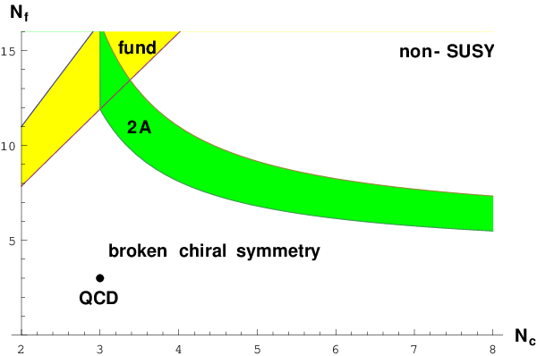
where . This expression is derived in appendix B using conformal anomaly matching. As alluded above, this expression does not lend itself to positivity because of the presence of the -point function. In this work, we will show that for gauge theories with gauge couplings only, the -point function term drops for theories in the conformal window cf. fig 1. This establishes the positivity with Euclidean methods and makes the evaluation more amenable to lattice simulations.

1.1 Executive Summary
In the remainder of this introduction, we give an executive summary of our work leaving the derivation of equations and definitions of schemes to the main part of the paper. Our assumptions are: (i) that the TEMT assumes the form
| (4) |
(summation over implied) and (ii) that the beta functions vanish in the IR & UV.33 3 For gauge theories with chiral symmetry breaking, the assumption breaks down since the goldstone bosons couple with a term which cannot be improved since it is in conflict with chiral symmetry [14, 15] leading to subtleties for flow theorems [16, 4]. Above operators with square brackets denote renormalised composite operators, e.g. in the case at hand, where , is the standard field strength tensor squared known from quantum chromodynamics (QCD). Using these assumptions allows us to derive
| (5) |
from (3). The -functions are -dependent through the couplings and the ’s are the analogues of the Zamolodchikov metric (cf. appendix A for definitions and notational conventions).44 4 Whereas the ’s are dependent on a generic scheme , the two flow integrals themselves are scheme independent, cf. [4]. We will refer to as the -metric throughout in a loose analogy to the Zamolodchikov metric in two dimensions. The expression (3) is derived in section 2, and is a new result of this paper.
For our work the crucial input is that the leading order correction to the non-interacting FP is
| (6) |
The main focus of this paper will be on asymptotically free QCD in the conformal window regime where (6) follows by using the conformal OPE (c.f. appendix C ) and is of course easily established by direct computation as well. Using (6) and our previous work on finiteness of - and -point functions we are able to define a scheme, referred to as the -scheme, for which along the flow. This establishes the main result of our paper
| (7) |
valid for the assumptions specified above and satisfying (6). On a side note this means that , for the same conditions, since the flow theorem for can be expressed in terms of the same -point function [4]. This relation was conjectured to hold for general classically conformal QFTs in [17]. In this work we show under what conditions this relation holds. A case where it fails is when the theory contains scalar couplings and the 3-point function does contribute.
The paper is organised as follows. The cornerstones, formula (5) and the scheme , are established in sections 2 and 3 respectively. More precisely, in section 3.1 it is shown that satisfies (6), used in section 3.2 to derive the finiteness of the counterterm which then allows the explicit construction of the scheme for which in section 3.3. Definitions, including notation from our previous work, are reviewed in appendix A. The sum rule (3) is derived in appendix B and a more formal argument for the first equation in (6), underlying the above mentioned scheme, is given in appendix C.
2 The Flow of (or ) as an Integral over the RG-scale
It is the aim of this section to derive (5). The presentation below is similar to the one given for the -flow in [4] where we have shown that55 5 For remarks concerning adding a local term to the bare action, with regards to eqns (3) and (8) cf. appendix B.2 or our previous work [4].
| (8) |
The starting point is formula (3), which is derived in appendix B. Using (8) one may write
| (9) |
where
| (10) |
and is defined in (B.10).66 6 Assuming the IR limit to be regular, we can choose to approach by taking, for example, and define a function .
The transformation of the equation above into an integral representation over the RG scale, necessitates the discussion of the renormalisation prescription. To regularise we use dimensional regularisation with . The correlator is renormalised by a splitting of the bare function into a renormalised and a counterterm
| (11) |
which consists in a Laurent series. Above (Källén function) and are the - and -point kinematic structures
| (12) |
where momentum conservation, , is implied. The quantities , are Laurent series in depending on the running couplings of the theory. From (9) it is seen that is the key quantity which we analyse by its scale dependence
| (13) |
In the last equality we used the result of [18] that is finite after resummation of divergences.
In establishing the flow formula (5), we follow the logic of [4] and introduce the so-called MOM-scheme, defined by
| (14) |
By solving the above ODE we arrive at
| (15) | |||||
where the split on the second line is compatible with (13). In order to pass to the coupling coordinates one uses the assumption (4) to write
| (16) |
with
| (17) |
Renormalisation of the above correlator and further definitions (e.g. in (A.8)) are reviewed in appendix A. It is now possible to define MOM-scheme relation analogical to (14) for the correlator (17). In this MOM-scheme we can use the relation , which in turn follows from substituting (4) into (14).
The final expression for is obtained by taking limit of (15) and inserting the result to (9)
| (18) |
Although as it stands (18) is written in a specific scheme, just like for [4], scheme-independence follow by observing that a change from a scheme to is given by a cohomologically trivial term
| (19) |
where with parametrising the change of scheme cf. eq. (A.10). This establishes the representation (5) and completes the aim of this section. We have also checked that eq. (18) is consistent with the -scheme formulae of [19] (namely 3.17b and 3.23 in this reference).
3 The -metric in Gauge Theories
In this section we restrict ourselves to QCD-like theories with one gauge coupling and massless fermions. The generalisation of the following result to multiple coupling theories satisfying (6) is straight forward. Before we proceed, let us establish the notation. The trace anomaly for gauge-theories reads
| (20) |
where is the logarithmic beta function. The corresponding operator is the field strength squared
| (21) |
with the somewhat non-standard treatment of the coupling constant (and has been defined previously). The mapping to the general expressions (5) and (7) is done by comparing (4) and (20), which gives and omitting the superscript on the -function for brevity.
In section 3.1 it is shown that , from where it is deduced, in section 3.2, that the counterterm to the -point function is finite when summed to all orders for all points along the flow. Based on this, in section 3.3, a scheme is defined for which , leading to the main result of the paper.
3.1 The vanishing of at the UV Fixed Point
Technically, we will show that . The -point function can be computed at leading order directly in momentum space by evaluating the diagram in fig. 2 which gives
| (22) | |||||
where the - and -point kinematic structures and are defined in (12). It is observed that at leading order in the coupling there is no divergent contribution to the -point function kinematic structure ; or more precisely to the projector (B.10) applied to the correlation function.

The -point function structure is not relevant for our work. From (11) and the definition of (A.8), follows. In principle this completes the task of this section but we think it is instructive to add a few more comments.
First, as demonstrated in the appendix C this can also be understood from the fact that for an exactly marginal operator the -structure vanishes in a CFT [20]. In the language of [20] the structure is referred to as semilocal, and that is at least one delta function in coordinate space; , in the case (22). For non-coincident points the correlation function is indeed proportional to cf. [21, 22]. It is in particular instructive to consider a case where this fails. An example is a free conformally coupled scalar field for which is an operator of scaling dimension four but since its perturbation induces an RG-flow, namely , it is not exactly marginal. In the explicit computation, one obtains in coordinate space
| (23) |
which is clearly not semi-local and will contribute to the structure upon Fourier transformation. On a side note it is a remarkable circumstance that from the evaluation (23), one can infer that the , cf. discussion in appendix C and [20].
Second, one might wonder whether something similar is possible for the -point function. The answer is no for the following reasons. If it were possible to set in some scheme then it would also imply that by reflection positivity in (8) which is incompatible with a non-trivial flow. The explicit straightforward computation for the -point function at leading order gives, , a non-contact term contribution, unlike (22), whose Fourier transform gives rise to -dependent term. Moreover, the formal argument given in appendix C does not descend to -point functions.
3.2 Finiteness of the 3-point Function
Following the analysis in [18], we study the finiteness of , the resummed Laurent series, after removing the regulator . This serves as the basis for defining the -scheme in the next section. The quantity is defined in analogy to in (11). In dimensional regularisation, the RGE (A.8) reads77 7 The quantity corresponds to in the classic paper of Jack and Osborn [19].
| (24) |
where we used the -dimensional logarithmic beta function and . This equation allows for the integral solution
| (25) |
This expression is well-defined for , convergent for , as we will show shortly for the asymptotically free and asymptotically safe case. Anticipating the result and removing regulator () the expression becomes
| (26) |
where the second integral representation in (26) is useful for practical computation.
- •
- •
We can also apply similar arguments for RG flows in the vicinity of a non-trivial UVFP , which corresponds to the asymptotically safe scenario (see [23] for some recent discussion of this possibility). In this case the UV behaviour is
(29) where and is the anomalous dimension of at the FP. One gets
(30) By inserting this back to (26), we find again finite UV behaviour . In fact, it is straightforward to see that provided , for any FP the equation (24) always allows for a finite solution
(31)
Let us now turn to the issue of IR convergence. Clearly, the presence of in the solution (26) indicates additional problems when the IR limit is taken. Note however, that near the IRFP another solution to (24) can be found
| (32) |
well-defined for . After taking (which is justified for the same reasons as (25)) one gets
| (33) |
By repeating the analysis leading to (27) and (28) near the IRFP, we conclude that (32) is well-defined in the vicinity of .
Assuming that the theory is free from any singularities in the coupling space, the solutions (25) and (32) should be compatible on overlapping domains. By subtracting (25) from (32) (and taking limit) we find a continuity condition
| (34) |
This is consistent with the vanishing of the 3-point contribution in (5), which can therefore be seen as the direct consequence of the finiteness and coupling continuity of . Indeed, in the next section, we will show how the above results can be used to construct a scheme, where the 3-metric vanishes.
3.3 Constructing the -scheme for the -metric
A change of scheme, cf. eq.(A.10), is given by a finite shift in the counterterms
| (35) |
Using (24) we can deduce that under such a shift the -metric transforms as
| (36) |
Since the limit of is uniform as shown in the previous section we can choose
| (37) |
to define a new scheme for which
| (38) |
is automatic. This scheme is new to this paper and not to be confused with the previously discussed MOM-scheme.
By using (38) in the general scheme-independent expression (18) we finally arrive at the desired result
| (39) |
We would like to end this section by demonstrating how to construct such a scheme in perturbation theory. Using the two-loop formulas of [19], we extract
| (40) |
where is one-loop coefficient of the beta function , the gluons and fermions are assumed to be in the adjoint and fundamental representation of an gauge group respectively (), and denotes the standard minimal subtraction scheme. By performing a scheme change (36) with
| (41) |
we achieve
| (42) |
as expected at this order in the perturbation theory. At the perturbative Banks-Zaks FP . Since is absent, in this theory can be computed purely by substituting the known perturbative expressions for the beta function and in (8) as was done up to five loops in [4] (see Eq. 60 and the discussion bellow in this reference).
To find at higher orders one would need to use the two-loop beta function together with the three-loop expression of , which is not presently available to the authors. Nevertheless, using the formulae of this paper some general predictions about the behaviour of these higher order corrections can be made (cf. appendix D).
After completion of the manuscript was computed to leading order in the large expansion in [24] by resumming infinite number of bubble diagrams. The result reads
| (43) |
where and
| (44) |
Since to leading order in the -function is one-loop exact , it is possible to use our formula (26) together with (37) to find the transformation corresponding to (43). The result reads
| (45) |
The formula above represents an application of our result beyond perturbation theory. By reexpanding expression (45) in small we find that the leading term agrees with (41).
4 Conclusions and Discussions
Our starting point was the derivation of a formula for the Euler anomaly or -function as an integral over the RG-scale of a - and -point functions of the trace of the energy momentum tensor (5), valid for theories which are governed by -functions at both fixed points (4).
For gauge theories in the conformal window the formula collapses to the -point function (7). Our main assumption for the proof is that the ultraviolet and infrared solution (25) and (32), of the RGE (24), can be matched continuously. This allowed us to define an explicit prescription, the -scheme (37), for which the -metric vanishes. In particular, our result means that for those theories, the Euler flow and the -flow are identical (8). The reason this works for gauge couplings, and not for generic couplings, is that for the former the -point function collapses to a -point function near the trivial FP (22). This is a consequence of the vanishing of the leading order contribution to the -metric (6) and can also be understood from the fact that the field strength tensor squared is an exactly marginal operator at zero coupling cf. appendix C. An example where this fails is a scalar free field theory for which is not an exactly marginal operator and its non-zero -function induces a -point function structure at leading order, prohibiting the use of the -scheme.
In the light of the above remarks one might wonder, whether the result can be applied to gauge theories with supersymmetry including scalar fields such as supersymmetric QCD (SQCD). The extension is possible owing the same form of the anomaly (4) in SQCD [25]. In supersymmetric gauge theories without superpotential the matter and gauge contributions are related through the Konishi anomaly [26], so that the trace anomaly can be expressed solely in terms of the field strength tensor squared up to equation of motion terms. We therefore expect that the main results of this paper should apply to SQCD in the conformal window.88 8 Some care has to be taken when passing from the dimensional regularisation to SUSY-preserving schemes (see Appendix A of [27] for some details of how this is to be done).

Another corollary of our analysis is that for the class of theories studied in this paper the strong -theorem applies. One defines the off-critical quantity
| (46) |
which reduces to in the limit by (39) and gives a (scheme dependent) interpolating function between the fixed points. The monotonicity of this function follows from the positivity of , established in [4].
Moreover, the perspective of implementing the -theorem in the conformal window on the lattice have improved since it is related to a -point function.99 9 This requires the renormalisation of the energy momentum tensor on the lattice which is a non-trivial task because of the breaking of the space-time symmetries [30]. Cf. [31, 32] for some recent proposals using the gradient flow technique. Supersymmetric lattice gauge theories [33], could be a particularly interesting test ground as the Euler anomaly is exactly known [34]. In practice though, lattice Monte Carlo simulation are done at finite quark mass which does not fall into our class of theories.1010 10 The TEMT contains a term of a the form in addition to the -function terms (4) where is the quark mass anomalous dimension. Thus unless this does not correspond to a CFT in the IR. A pragmatic way to deal with this problem is to choose an infrared cutoff ,
| (47) |
on the integral (7). The function is expected to plateau to for lower than the inverse quark mass for which the theory behaves like a massless theory.1111 11 None of this scales should be confused with the lattice size . In particular, , holds strictly by construction. To avoid finite size effects one has to impose as for the -point function the quark mass correction ought to be exponential where with is a mass of a hadron [35]. More precisely the flat region corresponds to the near-conformal behaviour in the vicinity of the IRFP. Thus one would expect to plateau to the massless case
| (48) |
for the above mentioned range, cf. fig.3 for a schematic illustration and an explanation about the scale . It would be interesting to apply this procedure to the case where the IR phase is chirally broken and investigate the expected appearance of the -divergence induced by the goldstone bosons [16, 4].
Acknowledgements
We are grateful to Luigi Del Debbio, José Latorre and Kostas Skenderis for useful discussions and Saad Nabeebaccus for careful reading of the manuscript. VP acknowledges the support of the Higgs Centre Edinburgh where a large part of this work was completed. VP is supported by the ERC STG grant 639220 (curvedsusy).
Appendix A Conventions for computing correlators
In this appendix we will give a brief review of the notation related to the renormalization of composite operator correlators adapted from [18].
We start with the -point functions of classically marginal renormalised operators
| (A.1) |
where the subtraction constant is a function of couplings of the theory and it contains Laurent series in as well as a finite part and is the finite renormalized correlator. A scheme is determined by the choice of the finite part of .
The finite quantity called Zamolodchikov metric is obtained via
| (A.2) |
where denotes the Lie derivative on a tensor in coupling space
| (A.3) |
Since the bare correlator is scale independent, the Zamolodchikov metric can be also defined directly from the finite renormalized correlators, e.g. [36], as follows
| (A.4) |
A scheme change is implemented using a finite, coupling dependent constant via
| (A.5) |
leaving the bare correlator invariant. Under such change we get a shift in the Zamolodchikov metric
| (A.6) |
The -point functions can be defined in a similar manner
| (A.7) | |||||
where cyclic permutation over the pairs , and is implied. Furthermore, , and are kinematic structures vanishing whenever any of the three external momenta is set to zero. Just as above and are subtraction constants containing Laurent series and finite parts. It follows that the -coefficients can be determined from the 2-point functions information (see [18] for the exact definition).
The new, purely 3-point information is encoded in the tensor. Again the scale derivative
| (A.8) |
proves useful. Above denotes the Lie derivative, acting on a -tensor
| (A.9) |
We can also define through the finite renormalized correlator by using a relation analogical to (A.4) and projecting onto etc.
The scheme change in is implemented via constant , which is now independent of from (A.6) (this follows since the structure is independent of the -point function). Under such scheme change we have and therefore
| (A.10) |
Appendix B Derivation of the 3-point Sum Rule
In this appendix, we provide a derivation of the -point sum rule (3) used in section 2 to derive a RG-scale integral representation for the Euler flow . Using the quantum action principle, a constraint on a gravity counterterm is worked out in section B.1, which is then used in the anomaly matching argument in section B.2 to derive the sum rule.
B.1 Renormalisation in Curved Space and
In an external gravitational field one needs to add counterterms
| (B.1) |
to the action to renormalise the theory [37]. The bare couplings are defined as etc. and geometric quantities are the same as in (2) except for which being a total derivative does not contribute to the action. The main idea is that the quantum action principle (differentiation with respect to sources) leads to finite quantities and thus to constraints on the counterterms. Concretely, a triple Weyl variation () leads to
| (B.2) |
where the abbreviation is introduced and we used (10) to include the dynamical contribution. By using, (11) we conclude that the finiteness of ensures finiteness of the combination in (B.2). Since has been shown to be finite [18] it is to be concluded that the quantity is finite. In particular this means that the limit is meaningful
| (B.3) |
In the last step we used that is finite and that . The latter follows from and the stationarity property at FPs (which can be seen by writing with constants and using ). Eq. (B.3) is a relevant observation as this implies finiteness of the corresponding term in the dilaton effective action.
B.2 Sum Rule from the Dilaton Effective Action
In the -point sum rule (3), the Euler flow arises, in dimensional regularisation, from an evanescent operator. This can be seen by writing the -dimensional Euler term as a sum of a four dimensional and an evanescent term
| (B.4) |
where we have assumed the conformally flat metric and is defined below (B.2). The -term is a total derivative
| (B.5) |
characteristic of topological terms. The evanescent part of the gravitational counterterms (B.1) becomes the Wess-Zumino term of the dilaton effective action in [6]
| (B.6) | |||||
where we have used (B.3). In the preceding argument, the finiteness of (and ) was essential to ensure UV finiteness of the dilaton effective action and match the the bare coefficient of the Wess-Zumino term to the Euler anomaly .
Similarly, the IR effective action contains the term which contributes at
| (B.7) |
We are now ready to put all the pieces together. By Fourier transforming the third functional derivative with respect to of (B.7), we see that at low momenta, the LHS of (B.2) behaves as
| (B.8) |
where the dots stand for nonlocal contributions subleading in the momentum expansion. Assuming momentum conservation, , (12) assumes the form
| (B.9) |
with the associated projector being
| (B.10) |
for which the -structure automatically vanishes (). Applying to the right-hand side of (B.2), one gets
| (B.11) |
where we used that for . The -point sum rule in momentum space follows
| (B.12) |
which in position space assumes the form
| (B.13) |
The Euler flow formula (B.13) is invariant under the addition of the local -term unlike the sum rule for (8) which needs to be amended. Such a scheme change (denoted as ’-scheme’ in [4]) should be viewed as independent of (A.6) and (A.10).1212 12 For more thorough discussion of various classes of schemes we refer the reader to [4], namely sections 2.3.2 and 2.3.3 of this reference. More concretely, the contribution of such shift precisely cancels between - and -point parts in (B.13). The reason this has to happen is that is well-defined at each FP and not only as a difference, like . At last, we would like to mention that eq. (B.13) itself has been derived by Anselmi [11] using different methods.
Appendix C Vanishing of at the UV Fixed Point - formal Argument
In this appendix we will demonstrate how in the free theory can be derived by using standard OPE arguments [38]. We start the discussion by considering a general perturbation
| (C.1) |
for some coupling constant that can be set to without loss of generality. We now deform the constant , the corrections to a generic correlator in the perturbed theory read
| (C.2) | |||||
The -term in (C.2) can be obtained by using the OPE
| (C.3) |
where dots encompass terms irrelevant for the calculation. By inserting this expression back into (C.2) and evaluating the integral with a UV cutoff , one finds that a logarithmic divergence appears
| (C.4) |
This divergence can be removed by adding a counterterm of the form
| (C.5) |
However, adding such a term amounts to introducing a -function
| (C.6) |
Hence the non-vanishing of the -function and the OPE coefficient are directly related.
We restrict our attention to the case at hand where in the free-field theory. Since the value of only affect the normalisation of the kinetic term, it is clear that the theory remains free (and therefore a CFT) for any value of . Thus and in the free theory
| (C.7) |
Using the fact that in a CFT the -point function of an operator is proportional to we conclude that also the -point function of has to vanish, which directly implies that
| (C.8) |
Note that the above argument shows that is exactly marginal at the Gaussian fixed point. In general an operator is called exactly marginal if its beta function vanishes, which is equivalent to the vanishing of the corresponding 3-point function as shown in [38, 20].1313 13 Note that the non-zero QCD -function should be understood as a consequence of coupling to fermions and gluons rather than a deformation by .
Appendix D The -scheme in Perturbation Theory
In this appendix, we will construct explicitly the solutions (26) and (32) for a theory with a trivial UVFP and a Banks-Zaks FP in the IR.
We start with the analysis near the trivial UVFP. The scheme (37) means that given a , we should be able to obtain to any given order in through (26). We demonstrate how this works for the first two non-vanishing orders in perturbation theory. Introducing the notation
| (D.1) |
the scheme change to is given by, performing the integral on the right-hand side of (26) and expanding the result in ,
| (D.2) |
where the two-loop -function is parameterised by . It is easily verified that
| (D.3) |
Note that (D.2) is and therefore nonzero at the UVFP even though itself vanishes there.
In the IR we assume a (Banks-Zaks) FP at , which exists for asymptotically free theory with . The -metric (D.1) expands to
| (D.4) |
where we used that for some finite constant (c.f. (40)). Close to this FP, (32) admits a perturbative solution in
| (D.5) |
Above we used that is the anomalous dimension of (field strength tensor squared). In the limit limit we get the expected dependence (31). Direct computation shows that (D.5) is compatible with (D.3). The leading parts of the IR solution (D.5) and the UV solution (D.2) match, up to corrections, provided that
| (D.6) |
The above should be regarded as the necessary condition for continuity of , equivalent to (34).
References
- [1] M. Duff, “Twenty years of the Weyl anomaly,” Class.Quant.Grav. 11 (1994) 1387–1404, arXiv:hep-th/9308075 [hep-th].
- [2] A. B. Zamolodchikov, “Irreversibility of the Flux of the Renormalization Group in a 2D Field Theory,” JETP Lett. 43 (1986) 730–732. [Pisma Zh. Eksp. Teor. Fiz.43,565(1986)].
- [3] J. L. Cardy, “The Central Charge and Universal Combinations of Amplitudes in Two-dimensional Theories Away From Criticality,” Phys. Rev. Lett. 60 (1988) 2709.
- [4] V. Prochazka and R. Zwicky, “On the Flow of Weyl-Anomaly,” Phys. Rev. D96 no. 4, (2017) 045011, arXiv:1703.01239 [hep-th].
- [5] J. L. Cardy, “Is There a c Theorem in Four-Dimensions?,” Phys. Lett. B215 (1988) 749–752.
- [6] Z. Komargodski and A. Schwimmer, “On Renormalization Group Flows in Four Dimensions,” JHEP 12 (2011) 099, arXiv:1107.3987 [hep-th].
- [7] Z. Komargodski, “The Constraints of Conformal Symmetry on RG Flows,” JHEP 07 (2012) 069, arXiv:1112.4538 [hep-th].
- [8] S. Forte and J. I. Latorre, “A Proof of the irreversibility of renormalization group flows in four-dimensions,” Nucl. Phys. B535 (1998) 709–728, arXiv:hep-th/9805015 [hep-th].
- [9] H. Osborn, “Derivation of a Four-dimensional Theorem,” Phys. Lett. B222 (1989) 97–102.
- [10] F. Baume, B. Keren-Zur, R. Rattazzi, and L. Vitale, “The local Callan-Symanzik equation: structure and applications,” JHEP 08 (2014) 152, arXiv:1401.5983 [hep-th].
- [11] D. Anselmi, “Kinematic sum rules for trace anomalies,” JHEP 11 (2001) 033, arXiv:hep-th/0107194 [hep-th].
- [12] K. A. Intriligator and N. Seiberg, “Lectures on supersymmetric gauge theories and electric-magnetic duality,” Nucl. Phys. Proc. Suppl. 45BC (1996) 1–28, arXiv:hep-th/9509066 [hep-th]. [,157(1995)].
- [13] C. T. Hill and E. H. Simmons, “Strong dynamics and electroweak symmetry breaking,” Phys. Rept. 381 (2003) 235–402, arXiv:hep-ph/0203079 [hep-ph]. [Erratum: Phys. Rept.390,553(2004)].
- [14] H. Leutwyler and M. A. Shifman, “GOLDSTONE BOSONS GENERATE PECULIAR CONFORMAL ANOMALIES,” Phys. Lett. B221 (1989) 384–388.
- [15] J. F. Donoghue and H. Leutwyler, “Energy and momentum in chiral theories,” Z. Phys. C52 (1991) 343–351.
- [16] M. A. Luty, J. Polchinski, and R. Rattazzi, “The -theorem and the Asymptotics of 4D Quantum Field Theory,” JHEP 01 (2013) 152, arXiv:1204.5221 [hep-th].
- [17] D. Anselmi, “Anomalies, unitarity and quantum irreversibility,” Annals Phys. 276 (1999) 361–390, arXiv:hep-th/9903059 [hep-th].
- [18] V. Prochazka and R. Zwicky, “Finiteness of two- and three-point functions and the renormalization group,” Phys. Rev. D95 no. 6, (2017) 065027, arXiv:1611.01367 [hep-th].
- [19] I. Jack and H. Osborn, “Analogs for the Theorem for Four-dimensional Renormalizable Field Theories,” Nucl.Phys. B343 (1990) 647–688.
- [20] A. Bzowski, P. McFadden, and K. Skenderis, “Scalar 3-point functions in CFT: renormalisation, beta functions and anomalies,” JHEP 03 (2016) 066, arXiv:1510.08442 [hep-th].
- [21] S. El-Showk, Y. Nakayama, and S. Rychkov, “What Maxwell Theory in D¡¿4 teaches us about scale and conformal invariance,” Nucl. Phys. B848 (2011) 578–593, arXiv:1101.5385 [hep-th].
- [22] F. A. Dolan and H. Osborn, “Conformal partial waves and the operator product expansion,” Nucl. Phys. B678 (2004) 491–507, arXiv:hep-th/0309180 [hep-th].
- [23] O. Antipin and F. Sannino, “Conformal Window 2.0: The large safe story,” Phys. Rev. D97 no. 11, (2018) 116007, arXiv:1709.02354 [hep-ph].
- [24] O. Antipin, N. A. Dondi, F. Sannino, and A. E. Thomsen, “The -theorem at large ,” arXiv:1808.00482 [hep-th].
- [25] M. A. Shifman and A. I. Vainshtein, “Solution of the Anomaly Puzzle in SUSY Gauge Theories and the Wilson Operator Expansion,” Nucl. Phys. B277 (1986) 456. [Zh. Eksp. Teor. Fiz.91,723(1986)].
- [26] K. Konishi, “Anomalous Supersymmetry Transformation of Some Composite Operators in SQCD,” Phys.Lett. B135 (1984) 439.
- [27] D. Z. Freedman and H. Osborn, “Constructing a c function for SUSY gauge theories,” Phys. Lett. B432 (1998) 353–360, arXiv:hep-th/9804101 [hep-th].
- [28] G. M. Pelaggi, F. Sannino, A. Strumia, and E. Vigiani, “Naturalness of asymptotically safe Higgs,” Front.in Phys. 5 (2017) 49, arXiv:1701.01453 [hep-ph].
- [29] D. F. Litim, M. Mojaza, and F. Sannino, “Vacuum stability of asymptotically safe gauge-Yukawa theories,” JHEP 01 (2016) 081, arXiv:1501.03061 [hep-th].
- [30] S. Caracciolo, G. Curci, P. Menotti, and A. Pelissetto, “The Energy Momentum Tensor for Lattice Gauge Theories,” Annals Phys. 197 (1990) 119.
- [31] H. Suzuki, “Energy–momentum tensor from the Yang–Mills gradient flow,” PTEP 2013 (2013) 083B03, arXiv:1304.0533 [hep-lat]. [Erratum: PTEP2015,079201(2015)].
- [32] L. Del Debbio, A. Patella, and A. Rago, “Space-time symmetries and the Yang-Mills gradient flow,” JHEP 11 (2013) 212, arXiv:1306.1173 [hep-th].
- [33] S. Catterall, D. B. Kaplan, and M. Unsal, “Exact lattice supersymmetry,” Phys. Rept. 484 (2009) 71–130, arXiv:0903.4881 [hep-lat].
- [34] D. Anselmi, D. Freedman, M. T. Grisaru, and A. Johansen, “Nonperturbative formulas for central functions of supersymmetric gauge theories,” Nucl.Phys. B526 (1998) 543–571, arXiv:hep-th/9708042 [hep-th].
- [35] L. Del Debbio and R. Zwicky, “Scaling relations for the entire spectrum in mass-deformed conformal gauge theories,” Phys. Lett. B700 (2011) 217–220, arXiv:1009.2894 [hep-ph].
- [36] G. M. Shore, The c and a-theorems and the Local Renormalisation Group. Springerbriefs in physics. Springer, Cham, 2017. arXiv:1601.06662 [hep-th].
- [37] S. Hathrell, “Trace Anomalies and QED in Curved Space,” Annals Phys. 142 (1982) 34.
- [38] L. P. Kadanoff and A. C. Brown, “Correlation functions on the critical lines of the Baxter and Ashkin-Teller models,” Annals Phys. 121 (1979) 318–342.