Model selection for sequential designs in discrete finite systems using Bernstein kernels
Abstract
We view sequential design as a model selection problem to determine which new observation is expected to be the most informative, given the existing set of observations. For estimating a probability distribution on a bounded interval, we use bounds constructed from kernel density estimators along with the estimated density itself to estimate the information gain expected from each observation. We choose Bernstein polynomials for the kernel functions because they provide a complete set of basis functions for polynomials of finite degree and thus have useful convergence properties. We illustrate the method with applications to estimating network reliability polynomials, which give the probability of certain sets of configurations in finite, discrete stochastic systems.
keywords
Bernstein polynomials, kernel density estimators, network reliability, sequential designs1 Introduction
The probability of configurations in a finite, discrete, stochastic dynamical system can be represented as a histogram with a finite number, , of bars. The bar heights are completely determined by a degree polynomial, but determining the coefficients of the monomial terms in the polynomial from data is notoriously ill-conditioned. Here we develop a numerically stable approach using an alternative basis of Bernstein polynomials instead of monomials and apply it to designing an efficient experiment to estimate the probability of configurations.
Given
- 1.
a function that can be represented as an degree polynomial and
- 2.
an “oracle” that can evaluate the function for arbitrary , but at a certain cost for each query,
we would like to find
- 1.
the sequence of points for querying the oracle such that each point gives the maximum amount of information about the function, i.e., most reduces the estimation error and
- 2.
a stopping criterion that lets the user decide when the amount of information to be gained is not worth the cost of calling the oracle, again.
We can project any degree polynomial uniquely onto the Bernstein basis of order ,
| (1) |
where is the th Bernstein basis function of order and are the Bernstein or Bézier coefficients (Bernstein, 1912; Levasseur, 1984; Lorentz, 2012). The function can thus be represented as a Bézier curve with control points . Bézier curves are frequently used in computer graphics, (Bézier et al., 1974; Farin, 1983; Bourke, 1996) in part because of the efficiency of de Casteljau’s recursive algorithm. It has been shown that de Casteljau’s algorithm is a numerically stable method for evaluating Bézier curves at arbitrary parameter values (De Casteljau, 1986; Chang and Rockwood, 1994; Phillips, 1997). A Bézier curve is completely contained in the convex hull of its control points and it always begins at the first control point and ends at the last one.
Bernstein polynomials have been extensively used to approximate a bounded and continuous function and adapted for smooth estimation of a distribution function concentrated on the interval (Babu et al., 2002; Comte and Lacour, 2011; Daouia et al., 2016). It has been shown that Bernstein estimators converge to the true densities for a degree polynomial (Petrone and Wasserman, 2002).
The function depends on the dynamical system. Further, the optimal -th measurement will typically depend on both the previous points and the values of the function at those points, making this an adaptive method. When the function is unknown, there is no guarantee of obtaining the most information possible out of every choice, but we propose a process that bounds the expected value of the information that is gained, given what we have already learned. Stopping criteria are determined by the Akaike Information Criterion () or Bayesian Information Criterion () applied to the L2 norm of successive estimates for . L2 norm provides our best estimate of the error in . If the error from the fit is within acceptable limits, we stop calling the oracle for additional points. The values of and give the information content of the estimator. Given a set of competing estimators to fit , the one with minimum and is preferred (Akaike, 1974; Akaike, 1998; Schwarz et al., 1978). We can view the model generated by each possible choice of measurement as a competing estimator and choose the measurement that provides the most marginal information. We will demonstrate these processes with two examples for which the function is known and consider the effect of estimation error in the coefficients themselves.
2 Method
For ease of explication, we focus on estimating a cumulative probability function of a single variable . Hence is monotonic non-decreasing, with and . Motivated by the typical behavior of the reliability polynomial for many stochastic systems, and without loss of generality, we introduce two parameters, and in our analysis, defined as follows: is the minimum for which and is the maximum such that . The corresponding s are and . In many applications, there are efficient methods for determining , and often their associated s, e.g., shortest path algorithms, minimum cut algorithms, and the Kirchoff matrix tree theorem. Out of the coefficients, now are unknown while the rest are s, s, and .
We call the estimator obtained with just these 4 parameters – and – the “estimator with no other knowledge”. There is an -parameter family of models consistent with these parameters. Bounds on can be obtained by choosing extremal values for the unknown s. A reasonable estimator, , can be obtained by linearly interpolating the unknown coefficients between the points and . The estimator is often surprisingly good. To improve the fit, the oracle is called to give a measurement of one of the unknown s and the remaining coefficients are again estimated using piecewise linear interpolation between the known coefficients. Knowledge of one more improves both the goodness-of-fit for and the bounds on . The optimization process allows us to select which measurement is likely to reduce the fitting error most. The process can be repeated till either all s have been measured by the oracle or the stopping criterion is reached.
We label the different estimators used in the process of estimating the exact as , where gives the number of additional known . is the “estimator with no additional knowledge”, is with one additional coefficient known i.e., in the toy example and so on. The goodness-of-fit is calculated by evaluating the L2 norm of :
| (2) | ||||
| (3) |
where s are the linearly interpolated ’s used to calculate . The integral of the Bernstein basis functions gives the factor . It is to be noted that is not simply the root-mean-squared error in the coefficients themselves. Cross terms appear because the Bernstein polynomials are not orthogonal. Also, the residuals for are the weighted smoothened version of those for . If the exact is unknown, we can nonetheless obtain provable bounds with the knowledge of the initial constraints and the values of and .

Now the aim is to determine which measurement by the oracle will most reduce the error in the estimation. Figure 1 shows the plot of the L2 norm obtained for the different as a function of for this case, where . For example, for the function described in Section 2.2, , and . The estimated for three possible choices of measurement, , and , are shown in Figures 2a, 2b and 2c, respectively.


By definition, we have the exact values and . In practice, the “oracle” is often a Monte Carlo simulation, and the cost of making a measurement can be exponential in the precision required. The cost may also depend on the value of , but we ignore that possibility here. Assuming that errors in are independent and identically distributed, we can estimate the distribution of by Monte Carlo. This gives the likelihood, that the observed data would be generated by the model . To calculate , we draw 10 random samples of values lying in the range (, ) from a binomial distribution (the sampling distribution of the Monte Carlo process used by the oracle) and obtain 10 different curves. We use the following equation to determine .
| (4) |
’s are the estimated coefficients obtained using linear interpolation, ’s and are the mean coefficients and the standard deviation respectively obtained from the 10 samples.
We consider the addition of more s as different models in this analysis and the one with the minimum and is chosen as the best candidate for fitting . Our models satisfy constraints on , the 4 basic parameters and some additional known . Therefore, the number of parameters estimated for each model is given by , where . The and values are calculated using
| (5) | ||||
| (6) |
where is the total number of points and is the maximum value of the likelihood function.
2.1 Toy Example
Consider the non-decreasing monotonic degree-7 polynomial 11 1 This is the reliability (Moore and Shannon, 1956) for the directed network , i.e., the probability that a message from node S will reach T if the probability of transmission is through each of the edges.,
| (7) |
which satisfies the boundary conditions, and . We can express it in the Bernstein basis as
| (8) |
where .
We start with the assumption that and are known. Figure 3a shows the bounds obtained from these known parameters. and must lie within these bounds. When we call the oracle to find one additional , both the fit and the bounds improve as shown in Figure 3b. Figures 3c and 3d show that improves with the additional and decreases from 0.0365 to 0.0047. The red points in Figure 3c and 3d represent the unknown linearly interpolated s which yield the red . The difference in the estimated ’s and with the exact ones are presented in Figure 3e and 3f.


The ’s for this small network can be evaluated exactly. However, if there were an error associated with the estimation of the s (those which are non-zero and not one), it could be handled by choosing random sets of s from the sampling distribution, as above. For example, if the errors are distributed uniformly in an interval around the observed value, the estimated would lie between the bounds shown in Figure 4.

2.2 Karate Network
The Zachary Karate club network (Zachary, 1977) is a social network of a university karate club, which has 34 vertices and 78 edges. This network has been extensively studied in the literature. Here we consider to be the probability that an infectious disease seeded in one randomly chosen person would eventually infect at least 30% of this population (i.e., at least 10 others), when the person-person transmission probability is 22 2 This is also a network reliability polynomial, which is related to the All Terminal reliability (Moore and Shannon, 1956; Youssef et al., 2013; Nath et al., 2018).. Figure 5 shows a high-precision Monte Carlo estimate of . For this network and this definition of reliability, , and . There are unknown lying between and .


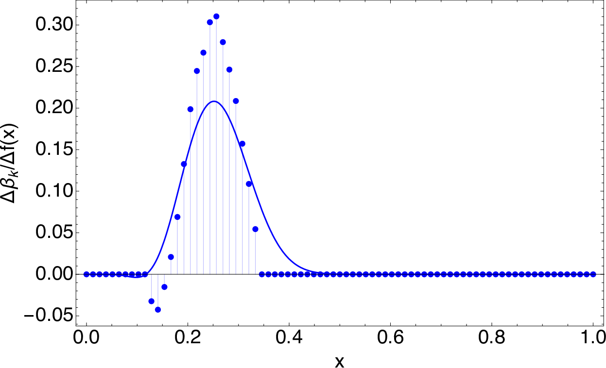

Table 1 summarizes the 6 models used for the analysis. The number of parameters estimated for each model, , is given by , where for this case. Similar to the example in Section 2.1, Figure 6 shows that knowing one more along with the initial 4 parameters - and , improves the estimate and the bounds of and that it makes a difference which is measured. The results for models 2-6 are in the Supplementary Material. Table 1 records the , and values for these models.
Model Estimator model 1 0 17 0.0694 model 2 1 16 0.0201 model 3 3 14 0.0074 model 4 5 12 0.0066 model 5 7 10 0.0012 model 6 9 8 0.0009
3 Discussions
Even when is unknown, we can bound it with the given information. Figures 1 and 2 show that the choice of at which to evaluate affects the quality of . Figure 1 also shows that if we could evaluate only one to estimate , we should pick for this particular example because it reduces the L2 norm the most. Figure 3 shows that the bounds on as well as the fit improve with additional measurements. The known s are used to calculate the unknown ones by linear interpolation. The estimated is obtained as a Bézier curve using these s. The black solid curve is the exact calculated using all the coefficients and the red is present within the bounds defined by the initial 4 parameters - and and the additional . This is demonstrated for a system with larger in Figure 6.
There will be an estimation error associated with the s obtained from Monte Carlo simulations for larger systems. Figure 4 show such an instance for the toy example when uniform error of 0.05 is assumed for all the s which are neither 0 nor 1. The resultant would lie within the bounded region. The error can be reduced by increasing the number of samples for the simulation yielding tighter bounds but this incurs possibly exponentially higher costs. Random samples for s obtained from the binomial Monte Carlo sampling distribution are used to calculate the likelihood that the true data has been generated by . The difference in the values from the random trials is plotted in the Supplementary Material.
The exact and estimated and the ’s for the Karate network for the various models listed in Table 1 are plotted in Figure 6. The in Table 1 decreases with the decrease in the number of estimated parameters. Since the standard deviation from the data is so small, the term dominates the information criteria, the number of parameters is actually irrelevant and it doesn’t matter which one of or is used. However, the change in or decreases monotonically with . Even though we do not obtain a minimum, it is still useful to calculate them because we place a threshold on what kind of error is tolerated. In practice, for some , it will drop below the threshold of bits per data point imposed by the cost of calling the oracle. For example, measuring only 7 of the 17 unknown s in the Karate network gives a good estimate of its reliability, as long as the right 7 are measured.
4 Conclusions
Many questions about finite, discrete stochastic systems can be answered by estimating the Moore Shannon network reliability, a probability distribution that is a high degree polynomial. Bernstein kernel density estimators provide extremely useful estimates for the overall reliability, when individual terms in the polynomial are estimated to arbitrary precision with Monte Carlo simulations. In addition, boundary conditions can often be used to specify many coefficients exactly. The corresponding Bézier curves can incorporate both the boundary constraints and simulation results. These Bernstein polynomials provide tight, provable bounds as well as achieving good estimates. We have shown here how these bounds can be used to guide a practical adaptive measurement process that efficiently uses calls to the Monte Carlo oracle to create a uniformly good approximation.
The number of samples required to reduce the error associated with precise measurements of the Bernstein coefficients using Monte Carlo simulations increases exponentially with the system size. The interplay between increasing the precision in estimates of individual s and increasing the number of s at which the s are measured remains to be investigated.
Acknowledgement
The authors would like to acknowledge Dr. Patrick Huber, Department of Physics, Virginia Tech. We thank our external collaborators and members of the Network Dynamics and Simulation Science Laboratory (NDSSL) for their suggestions and comments. This work has been partially supported by Defense Threat Reduction Agency Comprehensive National Incident Management System Contract HDTRA1-17-0118, by the National Institute of General Medical Sciences of the National Institutes of Health under a Models of Infectious Disease Agent Study (MIDAS) Grant U01GM070694 and by the United States Agency for International Development Grant AID-OAA-L-15-0001. The content is solely the responsibility of the authors and does not necessarily represent the official views of the National Institutes of Health, the Department of Defense or the United States Agency for International Development.
References
- Akaike (1974) Akaike, H. (1974) A new look at the statistical model identification. IEEE transactions on automatic control, 19, 716–723.
- Akaike (1998) — (1998) Information theory and an extension of the maximum likelihood principle. In Selected Papers of Hirotugu Akaike, 199–213. Springer.
- Babu et al. (2002) Babu, G. J., Canty, A. J. and Chaubey, Y. P. (2002) Application of Bernstein polynomials for smooth estimation of a distribution and density function. Journal of Statistical Planning and Inference, 105, 377 – 392. URL: http://www.sciencedirect.com/science/article/pii/S0378375801002658.
- Bernstein (1912) Bernstein, S. (1912) Démonstration du théoreme de weierstrass fondée sur le calcul des probabilities. Comm. Soc. Math. Kharkov, 13, 1–2.
- Bézier et al. (1974) Bézier, P. et al. (1974) Mathematical and practical possibilities of UNISURF. Computer Aided Geometric Design, 1.
- Bourke (1996) Bourke, P. (1996) Bézier curves. Bézier curves.
- Chang and Rockwood (1994) Chang, Y.-K. and Rockwood, A. P. (1994) A generalized de Casteljau approach to 3D free-form deformation. In Proceedings of the 21st annual conference on Computer graphics and interactive techniques, 257–260. ACM.
- Comte and Lacour (2011) Comte, F. and Lacour, C. (2011) Data-driven density estimation in the presence of additive noise with unknown distribution. Journal of the Royal Statistical Society: Series B (Statistical Methodology), 73, 601–627.
- Daouia et al. (2016) Daouia, A., Noh, H. and Park, B. U. (2016) Data envelope fitting with constrained polynomial splines. Journal of the Royal Statistical Society: Series B (Statistical Methodology), 78, 3–30.
- De Casteljau (1986) De Casteljau, P. D. F. (1986) Shape mathematics and CAD, vol. 2. Kogan Page.
- Farin (1983) Farin, G. (1983) Algorithms for rational Bézier curves. Computer-aided design, 15, 73–77.
- Levasseur (1984) Levasseur, K. M. (1984) A probabilistic proof of the Weierstrass approximation theorem. Amer. Math. Monthly, 91, 249–250.
- Lorentz (2012) Lorentz, G. G. (2012) Bernstein polynomials. American Mathematical Soc.
- Moore and Shannon (1956) Moore, E. and Shannon, C. (1956) Reliable circuits using less reliable relays. Journal of the Franklin Institute, 262, 191–208.
- Nath et al. (2018) Nath, M., Ren, Y., Khorramzadeh, Y. and Eubank, S. (2018) Determining whether a class of random graphs is consistent with an observed contact network. Journal of Theoretical Biology, 440, 121 – 132. URL: http://www.sciencedirect.com/science/article/pii/S002251931730560X.
- Petrone and Wasserman (2002) Petrone, S. and Wasserman, L. (2002) Consistency of Bernstein polynomial posteriors. Journal of the Royal Statistical Society: Series B (Statistical Methodology), 64, 79–100.
- Phillips (1997) Phillips, G. M. (1997) A de Casteljau algorithm for generalized Bernstein polynomials. BIT Numerical Mathematics, 37, 232–236.
- Schwarz et al. (1978) Schwarz, G. et al. (1978) Estimating the dimension of a model. The annals of statistics, 6, 461–464.
- Youssef et al. (2013) Youssef, M., Khorramzadeh, Y. and Eubank, S. (2013) Network reliability: The effect of local network structure on diffusive processes. Phys. Rev. E, 88, 052810. URL: https://link.aps.org/doi/10.1103/PhysRevE.88.052810.
- Zachary (1977) Zachary, W. W. (1977) An information flow model for conflict and fission in small groups. Journal of anthropological research, 33, 452–473.