All Transverse Motion is Peculiar: Connecting the Proper Motions of Galaxies to the Matter Power Spectrum

CAMB

Jeremy Darling Affiliation: Center for Astrophysics and Space Astronomy
Department of Astrophysical and Planetary Sciences
University of Colorado, 389 UCB
Boulder, CO 80309-0389, USA Corresponding author: Jeremy Darling Alexandra E. Truebenbach Affiliation: Center for Astrophysics and Space Astronomy
Department of Astrophysical and Planetary Sciences
University of Colorado, 389 UCB
Boulder, CO 80309-0389, USA

Abstract

In an isotropic and homogeneous Hubble expansion, all transverse motion is peculiar. Like the radial peculiar velocities of galaxies, transverse peculiar velocities are a means to trace the density of matter that does not rely on light tracing mass. Unlike radial peculiar velocity measurements that require precise redshift-independent distances in order to distinguish between the Hubble expansion and the observed redshift, transverse peculiar velocities can be measured using redshifts alone as a proxy for distance. Extragalactic proper motions can therefore directly measure peculiar velocities and probe the matter power spectrum. Here we develop two-point transverse velocity correlation statistics and demonstrate their dependence on the matter power spectrum. We predict the power in these correlation statistics as a function of the physical separation, angular separation, and distance of pairs of galaxies and demonstrate that the effect of large scale structure on transverse motions is best measured for pairs of objects with comoving separations less than about 50 Mpc. Transverse peculiar velocities induced by large scale structure should be observable as proper motions using long baseline radio interferometry or space-based optical astrometry.

Keywords:

astrometry — cosmology: observations — cosmology: theory — large-scale structure of universe — proper motions — techniques: high angular resolution

I Introduction

In a pure isotropic and homogeneous Hubble expansion, all apparent motion is radial. Therefore, proper motions of galaxies are the observable manifestation of peculiar velocities transverse to the line of sight induced by the density inhomogeneities of large scale structure. Extragalactic proper motions can be induced by a moving observer, an accelerating observer, or gravitational waves, which imprint a large-scale (dipole or quadrupole) proper motion signal on the sky [6, 2, 14, 4]. In contrast, the proper motion correlation of pairs of galaxies will imprint on all angular scales with a predictable dependence on pair separation that can be distinguished from these observer-induced signatures.

Studies of radial peculiar velocities require precise measurements of distances in order to disentangle the cosmological recession velocity from any peculiar velocity [13, 5, e.g.,]. Studies of transverse peculiar velocities, on the other hand, do not rely on accurate distance measurements and therefore, in principle, avoid a significant systematic error and can be made independent of cosmological model or extragalactic distance ladder. That said, proper motions are difficult to measure, particularly at the level that peculiar velocities are expected to arise: $v_{\rm pec}\sim 300$ km s^-1 is a proper motion of $\mu\sim 60$ $\mu$ as yr^-1 at 1 Mpc ( $\mu=v_{\rm pec}/D_{M}$ , neglecting the rate of change of the proper motion distance $D_{M}$ ). The distance at which transverse peculiar velocities could conceivably be measured in large astrometric surveys is about 100 Mpc, which is similar to radial peculiar velocity studies [16, e.g.,]. Measurements at much larger distances may be possible using gravitational lensing [9, 10, 11, e.g.].

Peculiar velocities relate directly to matter: it is gravity (dominated by dark matter) that drives peculiar motions. Unlike the two-point spatial correlation function, which depends strongly on small spatial scales, the peculiar velocity correlation functions get most of their power from larger spatial scales and therefore are better related to the linear density perturbation growth regime and more easily connected to the matter power spectrum [7, e.g.,].

Here we derive observable correlation statistics between pairs of extragalactic proper motions and relate these statistics to the matter power spectrum (Sections II and III). We explore observational strategies for detecting the peculiar velocities of galaxies induced by large scale structure in Section V. We parameterize the Hubble expansion today as $H_{0}=100$ $h$ km s^-1 Mpc^-1 and assume a geometrically flat universe with $\Omega_{m}=0.3$ and $\Omega_{\Lambda}=0.7$ .

II A Transverse Peculiar Velocity Correlation Function

Proper motions measure the transverse peculiar velocity, after observer-induced effects, such as the secular aberration drift and extragalactic parallax, and cosmological effects, such as primordial gravitational waves, are removed [6, 2, 3, 1, 14, 4]. But transverse velocities for different objects are not coplanar, so two-point correlations of pairs of transverse velocities will mix transverse and radial peculiar velocity correlation functions. This mixing of vector components in a spherical geometry is one reason why even 1D line-of-sight peculiar velocity studies are able to produce reasonable density maps [5, e.g.,].

We define a two-point correlation statistic $\xi_{v,\perp}$ that projects the transverse velocity of each object $\vec{v}_{\perp}(\vec{x}_{i})$ onto the space vector connecting the two objects, $\vec{x}=\vec{x}_{1}-\vec{x}_{2}$ , as

\xi_{v,\perp}(\vec{x}_{1},\vec{x}_{2})=\langle(\vec{v}_{\perp}(\vec{x}_{1})\cdot\hat{x})(\vec{v}_{\perp}(\vec{x}_{2})\cdot\hat{x})\rangle,

(1)

where the brackets indicate an average over all pairs with separation $|\vec{x}|$ . This statistic will produce negative values for pairs of objects that are converging or diverging along $\hat{x}$ and positive values for co-streaming motions. Unlike the radial peculiar velocity correlation function that depends directly on observable Doppler shifts $v(\vec{x}_{i})$ , $\xi_{v}(\vec{x}_{1},\vec{x}_{2})=\langle v(\vec{x}_{1})\,v(\vec{x}_{2})\rangle$ , two-dimensional transverse velocities must be reduced in dimensionality, and the choice for this reduction is non-unique. Since transverse velocities (observed as proper motions) of pairs of objects separated on the sky are not co-planar and are induced by the density inhomogeneities of large scale structure, we project the transverse velocities onto the space unit vector that connects the two objects, $\hat{x}$ . Another option is to simply take a dot product of the two transverse velocity vectors, $\xi^{\prime}_{v,\perp}(\vec{x}_{1},\vec{x}_{2})\equiv\langle\vec{v}_{\perp}(\vec{x}_{1})\cdot\vec{v}_{\perp}(\vec{x}_{2})\rangle$ (see Section IV for the derivation and results of this approach).

In what follows we connect this correlation statistic to the matter power spectrum in order to predict the correlated signals that should be observed in extragalactic proper motions and to connect observations to the matter power spectrum in a distance ladder-independent way. In Section II.1 we show that, in the linear regime of structure growth, which is a fair assumption for peculiar velocity statistics, Equation 1 can be reduced to two wavenumber integrals of the matter power spectrum and the derivatives of spherical Bessel functions:

	$\displaystyle\xi_{v,\perp}(\vec{x}_{1},\vec{x}_{2})=-f^{2}H_{0}^{2}\left[\sin^{2}\theta_{1}\sin^{2}\theta_{2}\ \int_{0}^{\infty}{dk\over 2\pi^{2}k}\ P(k)\ k\ j_{0}^{\prime\prime}(kx)\right.$
	$\displaystyle+\left.\frac{1}{4}\sin 2\theta_{1}\sin 2\theta_{2}\ \int_{0}^{\infty}{dk\over 2\pi^{2}k}\ P(k)\ {j_{0}^{\prime}(kx)\over x}\right].$		(2)

Terms are defined below.

II.1 Derivation

The following derivation is an adaptation of and closely follows the treatment of radial peculiar velocities by Dodelson [7] and relies on two assumptions: (1) linear growth of density perturbations $\delta=\delta\rho/\rho$ , which can be directly related to the Fourier components (spatial frequencies $\vec{k}$ ) of peculiar velocity at low redshift,

\vec{v}(\vec{k})=ifH_{0}\ \delta(\vec{k}){\vec{k}\over k^{2}},

(3)

where $f$ is the dimensionless linear growth rate approximated by $f=\Omega^{0.6}_{m}$ , and (2) low redshift, $z\lesssim 1$ .

Figure 1: The vectors and angles associated with a pair of objects with transverse velocities. The velocities have components out of the plane containing the two objects and the origin and are not necessarily coplanar.

D

is the distance to the pair midpoint,

\phi

is the pair vector orientation angle, and

\Delta\theta=\theta_{1}-\theta_{2}

Any velocity vector can be decomposed into radial and transverse components:

\vec{v}(\vec{x}_{i})=\vec{v}_{\perp}(\vec{x}_{i})+\vec{v}_{\parallel}(\vec{x}_{i})=\vec{v}_{\perp}(\vec{x}_{i})+(\vec{v}(\vec{x}_{i})\cdot\hat{x}_{i})\,\hat{x}_{i}

(4)

where $\hat{x}_{i}$ is the (radial) unit space vector to the object $i$ with velocity $\vec{v}(\vec{x}_{i})$ . The transverse velocity vector can therefore be expressed in terms of the total velocity vector and the direction to the object:

\vec{v}_{\perp}(\vec{x}_{i})=\vec{v}(\vec{x}_{i})-(\vec{v}(\vec{x}_{i})\cdot\hat{x}_{i})\,\hat{x}_{i}.

(5)

Inserting Equation 5 into the correlation statistic (Equation 1), we find that

\xi_{v,\perp}(\vec{x}_{1},\vec{x}_{2})=\langle\left(\left[\vec{v}(\vec{x}_{1})-(\vec{v}(\vec{x}_{1})\cdot\hat{x}_{1})\hat{x}_{1}\right]\cdot\hat{x}\right)\left(\left[\vec{v}(\vec{x}_{2})-(\vec{v}(\vec{x}_{2})\cdot\hat{x}_{2})\hat{x}_{2}\right]\cdot\hat{x}\right)\rangle.

(6)

Defining angles $\theta_{1}$ and $\theta_{2}$ in terms of the projections of $\hat{x}_{1}$ and $\hat{x}_{2}$ onto $\hat{x}$ (Figure 1), $\cos\theta_{1}\equiv-\hat{x}_{1}\cdot\hat{x}$ and $\cos\theta_{2}\equiv-\hat{x}_{2}\cdot\hat{x}$ ,¹¹ 1 These slightly unusual definitions arise from the definition $\vec{x}=\vec{x}_{1}-\vec{x}_{2}$ , the dot product $\hat{x}_{i}\cdot\hat{x}=\cos(\pi-\theta_{i})=-\cos\theta_{i}$ and the requirement that the observed angle between the two objects be $\Delta\theta=\theta_{1}-\theta_{2}$ . See Figure 1. and expanding the dot products,

\xi_{v,\perp}(\vec{x}_{1},\vec{x}_{2})=\langle\left(\vec{v}(\vec{x}_{1})\cdot\hat{x}+\vec{v}(\vec{x}_{1})\cdot\hat{x}_{1}\cos\theta_{1}\right)\left(\vec{v}(\vec{x}_{2})\cdot\hat{x}+\vec{v}(\vec{x}_{2})\cdot\hat{x}_{2}\cos\theta_{2}\right)\rangle.

(7)

This expression expands into four parts that can be treated separately:

	$\displaystyle\xi_{v,\perp}(\vec{x}_{1},\vec{x}_{2})=\langle\overbrace{(\vec{v}(\vec{x}_{1})\cdot\hat{x})(\vec{v}(\vec{x}_{2})\cdot\hat{x})}^{(i)}\rangle+\langle\overbrace{(\vec{v}(\vec{x}_{1})\cdot\hat{x})(\vec{v}(\vec{x}_{2})\cdot\hat{x}_{2}\cos\theta_{2})}^{(ii)}\rangle+\langle\overbrace{(\vec{v}(\vec{x}_{2})\cdot\hat{x})(\vec{v}(\vec{x}_{1})\cdot\hat{x}_{1}\cos\theta_{1})}^{(iii)}\rangle$
	$\displaystyle+\langle\overbrace{(\vec{v}(\vec{x}_{1})\cdot\hat{x}_{1})(\vec{v}(\vec{x}_{2})\cdot\hat{x}_{2})\cos\theta_{1}\cos\theta_{2}}^{(iv)}\rangle.$		(8)

For each part of this expression (following Dodelson [7]), we recast the velocity vectors in terms of their Fourier components,

\vec{v}(\vec{x}_{i})=\int{d^{3}k\over(2\pi)^{3}}\ e^{i\vec{k}\cdot\vec{x}_{i}}\ \vec{v}(\vec{k}),

(9)

and employ linear theory for $\vec{v}(\vec{k})$ to relate it to the density perturbation $\delta(\vec{k})$ (Equation 3).

II.1.1 Part $(i)$

Part $(i)$ is the transverse counterpart to the radial peculiar velocity two point correlation function, $\xi_{v}(\vec{x}_{1},\vec{x}_{2})=\langle(\vec{v}(\vec{x}_{1})\cdot\hat{x}_{1})\,(\vec{v}(\vec{x}_{2})\cdot\hat{x}_{2})\rangle$ . Rather than projecting the 3D velocities onto the radial coordinate, $(i)$ projects the 3D velocities onto the vector connecting the two objects, $\hat{x}$ . For pairs of objects with small angular separations, $\hat{x}$ be nearly coplanar with the observed proper motion vectors.

Using the Fourier transforms of the velocity vectors (Eqn. 9) followed by the linear velocity-density relation (Eqn. 3), part $(i)$ of the correlation statistic becomes

	$\displaystyle\langle(\vec{v}(\vec{x}_{1})\cdot\hat{x})(\vec{v}(\vec{x}_{2})\cdot\hat{x})\rangle$	$\displaystyle=$	$\displaystyle\int{d^{3}k\over(2\pi)^{3}}\ e^{i\vec{k}\cdot\vec{x}_{1}}\int{d^{3}k^{\prime}\over(2\pi)^{3}}\ e^{-i\vec{k}^{\prime}\cdot\vec{x}_{2}}\ \langle(\vec{v}(\vec{k})\cdot\hat{x})(\vec{v}^{\,*}(\vec{k}^{\prime})\cdot\hat{x})\rangle$		(10)
		$\displaystyle=$	$\displaystyle f^{2}H_{0}^{2}\ \int{d^{3}k\over(2\pi)^{3}}\ e^{i\vec{k}\cdot\vec{x}_{1}}\int{d^{3}k^{\prime}\over(2\pi)^{3}}\ e^{-i\vec{k}^{\prime}\cdot\vec{x}_{2}}\ \langle\delta(\vec{k})\delta^{*}(\vec{k}^{\prime})\rangle{(\vec{k}\cdot\hat{x})(\vec{k}^{\prime}\cdot\hat{x})\over k^{2}k^{\prime\,2}}.$		(11)

Using what is often the definition of the matter power spectrum, $P(k)$ , in terms of the density fluctuation variance and the Dirac delta function $\delta^{3}(\vec{k}-\vec{k}^{\prime})$ ,

\langle\delta(\vec{k})\delta^{*}(\vec{k}^{\prime})\rangle=(2\pi)^{3}\delta^{3}(\vec{k}-\vec{k}^{\prime})P(k),

(12)

we can reduce part $(i)$ to integrals in a single wavenumber:

\langle(\vec{v}(\vec{x}_{1})\cdot\hat{x})(\vec{v}(\vec{x}_{2})\cdot\hat{x})\rangle=f^{2}H_{0}^{2}\ \int_{0}^{\infty}{dk\,k^{2}\over(2\pi)^{3}}\ P(k)\int d\Omega_{k}\ e^{i\vec{k}\cdot\vec{x}}\ {(\vec{k}\cdot\hat{x})^{2}\over k^{4}}.

(13)

Since the wavenumber can be written

\vec{k}=e^{-i\vec{k}\cdot\vec{x}}\ {1\over i}\,\frac{\partial}{\partial\vec{x}}\,e^{i\vec{k}\cdot\vec{x}}\ ,

(14)

using index notation and the Einstein convention, we have

e^{i\vec{k}\cdot\vec{x}}\ (\vec{k}\cdot\hat{x})(\vec{k}\cdot\hat{x})=-\hat{x}_{i}\hat{x}_{j}\frac{\partial^{2}}{\partial x_{i}\partial x_{j}}e^{i\vec{k}\cdot\vec{x}}

(15)

and part $(i)$ becomes

\langle(\vec{v}(\vec{x}_{1})\cdot\hat{x})(\vec{v}(\vec{x}_{2})\cdot\hat{x})\rangle=-f^{2}H_{0}^{2}\ \int_{0}^{\infty}{dk\over(2\pi)^{3}k^{2}}\ P(k)\ \hat{x}_{i}\hat{x}_{j}\frac{\partial^{2}}{\partial x_{i}\partial x_{j}}\int d\Omega_{k}\ e^{i\vec{k}\cdot\vec{x}}.

(16)

At this stage, the only difference between $\xi_{v}(\vec{x}_{1},\vec{x}_{2})$ and the above are the unit vectors: for the radial peculiar velocity correlation function, these are the radial unit vectors $\hat{x}_{1}$ and $\hat{x}_{2}$ [7], while for part $(i)$ of the transverse peculiar velocity correlation function, it is the unit vector $\hat{x}$ . The angular integral is

\int d\Omega_{k}\ e^{i\vec{k}\cdot\vec{x}}=\int_{0}^{2\pi}d\phi\int_{-1}^{+1}d\mu\ e^{ikx\mu}=4\pi j_{0}(kx)

(17)

where $j_{0}(kx)=\sin(kx)/kx$ is the $\ell=0$ spherical Bessel function. The derivatives with respect to the components of $\vec{x}$ can be rewritten in terms of derivatives of the argument of $j_{0}$ , $kx$ :

\frac{\partial^{2}}{\partial x_{i}\partial x_{j}}j_{0}(kx)=k^{2}\left(\left[\delta_{ij}-\hat{x}_{i}\hat{x}_{j}\right]{j_{0}^{\prime}(kx)\over kx}+\hat{x}_{i}\hat{x}_{j}j_{0}^{\prime\prime}(kx)\right).

(18)

Thus,

\langle(\vec{v}(\vec{x}_{1})\cdot\hat{x})(\vec{v}(\vec{x}_{2})\cdot\hat{x})\rangle=-f^{2}H_{0}^{2}\ \int_{0}^{\infty}{dk\over 2\pi^{2}}\ P(k)\ \hat{x}_{i}\hat{x}_{j}\left(\left[\delta_{ij}-\hat{x}_{i}\hat{x}_{j}\right]{j_{0}^{\prime}(kx)\over kx}+\hat{x}_{i}\hat{x}_{j}j_{0}^{\prime\prime}(kx)\right)

(19)

Summing over $i$ and $j$ causes the $j_{0}^{\prime}(kx)$ term to vanish. We will label this result for part $(i)$ $\xi_{v,(i)}$ :

\xi_{v,(i)}(x)=-f^{2}H_{0}^{2}\ \int_{0}^{\infty}{dk\over 2\pi^{2}k}\ P(k)\ k\ j_{0}^{\prime\prime}(kx).

(20)

It is instructive to examine the behavior of $P(k)$ , $j_{0}^{\prime\prime}(kx)$ , and the integral of their product, which we will do below (Section II.1.5).

II.1.2 Part $(ii)$

For part $(ii)$ , we have

$\displaystyle\langle(\vec{v}(\vec{x}_{1})\cdot\hat{x})(\vec{v}(\vec{x}_{2})\cdot\hat{x}_{2}\cos\theta_{2})\rangle$	$\displaystyle=$	$\displaystyle\int{d^{3}k\over(2\pi)^{3}}\ e^{i\vec{k}\cdot\vec{x}_{1}}\int{d^{3}k^{\prime}\over(2\pi)^{3}}\ e^{-i\vec{k}^{\prime}\cdot\vec{x}_{2}}\ \langle(\vec{v}(\vec{k})\cdot\hat{x})(\vec{v}^{\,*}(\vec{k}^{\prime})\cdot\hat{x}_{2}\cos\theta_{2})\rangle$	(21)
	$\displaystyle=$	$\displaystyle f^{2}H_{0}^{2}\ \int{d^{3}k\over(2\pi)^{3}}\ e^{i\vec{k}\cdot\vec{x}_{1}}\int{d^{3}k^{\prime}\over(2\pi)^{3}}\ e^{-i\vec{k}^{\prime}\cdot\vec{x}_{2}}\ \langle\delta(\vec{k})\delta^{*}(\vec{k}^{\prime})\rangle{(\vec{k}\cdot\hat{x})(\vec{k}^{\prime}\cdot\hat{x}_{2})\cos\theta_{2}\over k^{2}k^{\prime\,2}}$	(22)
	$\displaystyle=$	$\displaystyle f^{2}H_{0}^{2}\ \int_{0}^{\infty}{dk\,k^{2}\over(2\pi)^{3}}\ P(k)\int d\Omega_{k}\ e^{i\vec{k}\cdot\vec{x}}\ {(\vec{k}\cdot\hat{x})(\vec{k}\cdot\hat{x}_{2})\cos\theta_{2}\over k^{4}}$	(23)
	$\displaystyle=$	$\displaystyle-f^{2}H_{0}^{2}\ \int_{0}^{\infty}{dk\over(2\pi)^{3}k^{2}}\ P(k)\ \hat{x}_{i}\hat{x}_{2,j}\cos\theta_{2}\ \frac{\partial^{2}}{\partial x_{i}\partial x_{j}}\int d\Omega_{k}\ e^{i\vec{k}\cdot\vec{x}}$	(24)
	$\displaystyle=$	$\displaystyle-f^{2}H_{0}^{2}\ \int_{0}^{\infty}{dk\over 2\pi^{2}}\ P(k)\ \hat{x}_{i}\hat{x}_{2,j}\cos\theta_{2}\ \left(\left[\delta_{ij}-\hat{x}_{i}\hat{x}_{j}\right]{j_{0}^{\prime}(kx)\over kx}+\hat{x}_{i}\hat{x}_{j}j_{0}^{\prime\prime}(kx)\right)$	(25)
	$\displaystyle=$	$\displaystyle-f^{2}H_{0}^{2}\ \int_{0}^{\infty}{dk\over 2\pi^{2}}\ P(k)\ (\hat{x}_{2}\cdot\hat{x})\cos\theta_{2}\ j_{0}^{\prime\prime}(kx).$	(26)

Since $\hat{x}_{2}\cdot\hat{x}=-\cos\theta_{2}$ , we obtain an expression for part $(ii)$ that is very similar to the result for part $(i)$ modulo a factor of $-\cos^{2}\theta_{2}$ :

	$\displaystyle\langle(\vec{v}(\vec{x}_{1})\cdot\hat{x})(\vec{v}(\vec{x}_{2})\cdot\hat{x}_{2}\cos\theta_{2})\rangle$	$\displaystyle=$	$\displaystyle+\cos^{2}\theta_{2}\ f^{2}H_{0}^{2}\ \int_{0}^{\infty}{dk\over 2\pi^{2}k}\ P(k)\ k\ j_{0}^{\prime\prime}(kx)$		(27)
		$\displaystyle=$	$\displaystyle-\cos^{2}\theta_{2}\ \xi_{v,(i)}(x).$		(28)

II.1.3 Part $(iii)$

Part $(iii)$ has a nearly identical result to part $(ii)$ :

\langle(\vec{v}(\vec{x}_{2})\cdot\hat{x})(\vec{v}(\vec{x}_{1})\cdot\hat{x}_{1}\cos\theta_{1})\rangle=-\cos^{2}\theta_{1}\ \xi_{v,(i)}(x).

(29)

II.1.4 Part $(iv)$

Part $(iv)$ follows the same procedure until the stage where we sum over $i$ and $j$ :

$\displaystyle\langle(\vec{v}(\vec{x}_{1})\cdot\hat{x}_{1})($	$\displaystyle\vec{v}(\vec{x}_{2})$	$\displaystyle\cdot\hat{x}_{2})\cos\theta_{1}\cos\theta_{2}\rangle$	(30)
	$\displaystyle=$	$\displaystyle-f^{2}H_{0}^{2}\int_{0}^{\infty}{dk\over 2\pi^{2}}\ P(k)\,\hat{x}_{1,i}\hat{x}_{2,j}\cos\theta_{1}\cos\theta_{2}\left(\left[\delta_{ij}-\hat{x}_{i}\hat{x}_{j}\right]{j_{0}^{\prime}(kx)\over kx}+\hat{x}_{i}\hat{x}_{j}j_{0}^{\prime\prime}(kx)\right)$	(30)
	$\displaystyle=$	$\displaystyle-f^{2}H_{0}^{2}\int_{0}^{\infty}{dk\over 2\pi^{2}}\ P(k)\,\cos\theta_{1}\cos\theta_{2}\left(\left[\cos(\theta_{1}-\theta_{2})-\cos\theta_{1}\cos\theta_{2}\right]{j_{0}^{\prime}(kx)\over kx}+\cos\theta_{1}\cos\theta_{2}j_{0}^{\prime\prime}(kx)\right)$	(31)
	$\displaystyle=$	$\displaystyle-f^{2}H_{0}^{2}\int_{0}^{\infty}{dk\over 2\pi^{2}k}\ P(k)\,\left(\sin\theta_{1}\sin\theta_{2}\cos\theta_{1}\cos\theta_{2}\ {j_{0}^{\prime}(kx)\over x}+\cos^{2}\theta_{1}\cos^{2}\theta_{2}\ k\ j_{0}^{\prime\prime}(kx)\right),$	(32)

where $\cos(\theta_{1}-\theta_{2})=\hat{x}_{1}\cdot\hat{x}_{2}$ , which comes from the inner angles of the $\vec{x}_{1}$ - $\vec{x}_{2}$ - $\vec{x}$ triangle, is invoked in Equation 31. We define $\xi_{v,(iv)}(x)$ to be the integral involving $j_{0}^{\prime}(kx)$ to obtain an expression for part $(iv)$ :

\langle(\vec{v}(\vec{x}_{1})\cdot\hat{x}_{1})(\vec{v}(\vec{x}_{2})\cdot\hat{x}_{2})\cos\theta_{1}\cos\theta_{2}\rangle=\sin\theta_{1}\sin\theta_{2}\cos\theta_{1}\cos\theta_{2}\ \xi_{v,(iv)}(x)+\cos^{2}\theta_{1}\cos^{2}\theta_{2}\ \xi_{v,(i)}(x).

(33)

Refer to caption — Figure 2: Top Left: Integration kernels for the transverse peculiar velocity correlation function (Equation 35) versus wavenumber for objects separated by $x=50$ $h^{-1}$ Mpc. Top Right: Matter power spectrum $P(k)$ versus wavenumber obtained from CAMB (Section II.1.5). Bottom Left: Matter power spectrum modulated by the integration kernels for $x=50$ $h^{-1}$ Mpc. Bottom Right: Integrated modulated power spectrum (the two terms in Equation 34, omitting the prefactors on $\xi_{v,(i)}$ and $\xi_{v,(iv)}$ ) versus pair separation $x$ .

II.1.5 Sum of Parts

Summing all parts of Equation 8, we have

\xi_{v,\perp}(\vec{x}_{1},\vec{x}_{2})=\sin^{2}\theta_{1}\sin^{2}\theta_{2}\ \xi_{v,(i)}(x)+\frac{1}{4}\sin 2\theta_{1}\sin 2\theta_{2}\ \xi_{v,(iv)}(x)

(34)

	$\displaystyle\xi_{v,\perp}(\vec{x}_{1},\vec{x}_{2})=-f^{2}H_{0}^{2}\left[\sin^{2}\theta_{1}\sin^{2}\theta_{2}\ \int_{0}^{\infty}{dk\over 2\pi^{2}k}\ P(k)\ k\ j_{0}^{\prime\prime}(kx)\right.$
	$\displaystyle+\left.\frac{1}{4}\sin 2\theta_{1}\sin 2\theta_{2}\ \int_{0}^{\infty}{dk\over 2\pi^{2}k}\ P(k)\ {j_{0}^{\prime}(kx)\over x}\right].$		(35)

The $\xi_{v,(i)}(x)$ term represents the motion along the pair separation axis $\hat{x}$ , and the $\xi_{v,(iv)}(x)$ term represents the motion perpendicular to $\hat{x}$ (defining a plane). It is instructive to examine the two kernels in this expression to see where most of the power lies in the correlation of transverse peculiar velocities. Figure 2 (top left) shows the integration kernels for the two terms above, assuming $x=50$ $h^{-1}$ Mpc. While power will be included on all scales, there is a suppression of power on spatial frequencies $k\gtrsim 0.1$ $h$ Mpc^-1. As with the radial velocity correlation function, the transverse velocity correlation is less sensitive to the nonlinear density perturbation regime than the density correlation function.

Figure 2 (top right) shows the matter power spectrum $P(k)$ obtained from the online Code for Anisotropies in the Microwave Background (CAMB)²² 2 Lewis, A. & Challinor, A., August 2017 version. for $z=0$ , $H_{0}=70$ km s^-1 Mpc^-1, $\Omega_{b}=0.0462$ , $\Omega_{CDM}=0.2538$ , and $\Omega_{\Lambda}=0.7$ . Figure 2 (bottom left) shows the kernel-weighted power spectrum for each term $\xi_{v,(i)}$ and $\xi_{v,(iv)}$ versus wavenumber $k$ . Figure 2 (bottom right) shows the wavenumber-integrated kernel-weighted power spectrum for each term $\xi_{v,(i)}$ and $\xi_{v,(iv)}$ in Equation 34 (omitting prefactors, which depend on individual pairs) versus physical separation $x$ . It should be stressed that while these terms in the transverse peculiar velocity correlation function peak at the smallest pair separations, the scales driving the correlated motions are dominated by much larger scale structure, $k\lesssim 0.1$ $h$ Mpc^-1. For example, a fairly close pair of galaxies will show highly correlated peculiar motion as they both respond to the density enhancement of the local filament or supercluster.

III Results

III.1 Equidistant Pairs

It is instructive to examine the above results for equidistant pairs of objects, $|\vec{x}_{1}|=|\vec{x}_{2}|$ , which implies that $\theta_{1}=\pi-\theta_{2}$ and $\Delta\theta=\theta_{1}-\theta_{2}=\pi-2\theta_{2}=2\theta_{1}-\pi$ . In this special case, Equation 34 simplifies to

\xi_{v,\perp}(\vec{x}_{1},\vec{x}_{2})\Bigr\rvert_{|\vec{x}_{1}|=|\vec{x}_{2}|}=\cos^{4}{\Delta\theta\over 2}\ \xi_{v,(i)}(x)-\frac{1}{4}\sin^{2}\Delta\theta\ \xi_{v,(iv)}(x).

(36)

Figure 3 shows this correlation function versus pair physical separation and versus pair angular separation. Pairs of objects with smaller physical separations, $x\lesssim 50$ Mpc, and smaller angular separations, $\Delta\theta\lesssim 60^{\circ}$ , show the largest transverse velocity correlation. The positive value of the correlation in these cases indicates co-streaming motions induced by density inhomogeneities (negative values would indicate converging or diverging motions, as is seen at low amplitude for large angular separations in Figure 3.

Equation 36 can be rewritten in terms of the ratio of the physical separation of pairs $x$ to the radial distance to each object ( $x_{1}=|\vec{x}_{1}|=|\vec{x}_{2}|$ ):

\xi_{v,\perp}(\vec{x}_{1},\vec{x}_{2})\Bigr\rvert_{|\vec{x}_{1}|=|\vec{x}_{2}|}=\left[1-\left({x\over 2x_{1}}\right)^{2}\right]^{2}\xi_{v,(i)}(x)-\left[1-\left({x\over 2x_{1}}\right)^{2}\right]\left({x\over 2x_{1}}\right)^{2}\xi_{v,(iv)}(x).

(37)

When the two objects in a pair are equidistant, the largest possible pair separation is twice the distance to each object ( $\Delta\theta=\pi$ ), and the smallest possible distance is half of the pair separation. When these extremal conditions are met, the projection of the transverse velocities onto $\hat{x}$ is zero and the correlation is null. On the other hand, when pairs have separations that are small compared to their distance, $\Delta\theta$ is small and the correlation asymptotes to $\xi_{v,(i)}(x)$ . Figure 4 (right) demonstrates that for $x_{1}\gtrsim 4x$ , the correlation becomes nearly constant at its largest amplitude.

III.2 Randomly Oriented Pairs

Equidistant pairs represent a special case of the physical reality of randomly oriented pairs. For fixed separation, we can examine the ensemble average of randomly oriented pair separation vector $\hat{x}$ using Equation 34. In this case, $\theta_{1}$ and $\theta_{2}$ are not independent random variables; they are determined by the orientation of the pair axis and the ratio of the pair separation $x$ to the distance to the pair midpoint $D$ :

	$\displaystyle\sin\theta_{1}$	$\displaystyle=$	$\displaystyle{\sin\phi\over\sqrt{1+{x\over D}\cos\phi+{1\over 4}\left(x\over D\right)^{2}}}$		(38)
	$\displaystyle\sin\theta_{2}$	$\displaystyle=$	$\displaystyle{\sin\phi\over\sqrt{1-{x\over D}\cos\phi+{1\over 4}\left(x\over D\right)^{2}}}.$		(39)

The orientation of the pair axis is determined by the angle $\phi$ , which we choose to be zero when $\hat{x}$ is radial (along the line of sight) and $\vec{x}_{1}>\vec{x}_{2}$ (see Figure 1). Random pair orientation corresponds to a uniform distribution in $\phi\ \epsilon\ [0,\pi]$ .

Using Equations 38 and 39, the angular terms in Equation 34 can be expressed in therms of $\phi$ and $x/D$ :

	$\displaystyle\sin^{2}\theta_{1}\sin^{2}\theta_{2}$	$\displaystyle=$	$\displaystyle{\sin^{4}\phi\over 1+\left({x\over D}\right)^{2}\left(\sin^{2}\phi-{1\over 2}\right)+{1\over 16}\left(x\over D\right)^{4}}$		(40)
	$\displaystyle{1\over 4}\sin 2\theta_{1}\sin 2\theta_{2}$	$\displaystyle=$	$\displaystyle{\left(1-{1\over 4}\left(x\over D\right)^{2}\right)\sin^{2}\phi-\sin^{4}\phi\over 1+\left({x\over D}\right)^{2}\left(\sin^{2}\phi-{1\over 2}\right)+{1\over 16}\left(x\over D\right)^{4}}.$		(41)

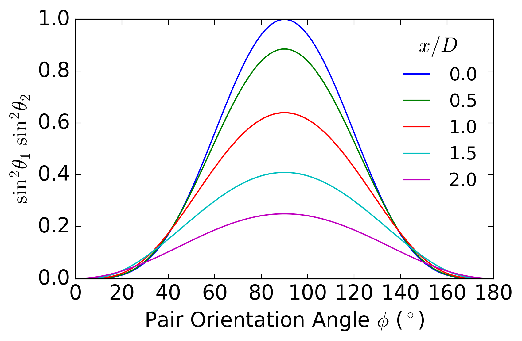
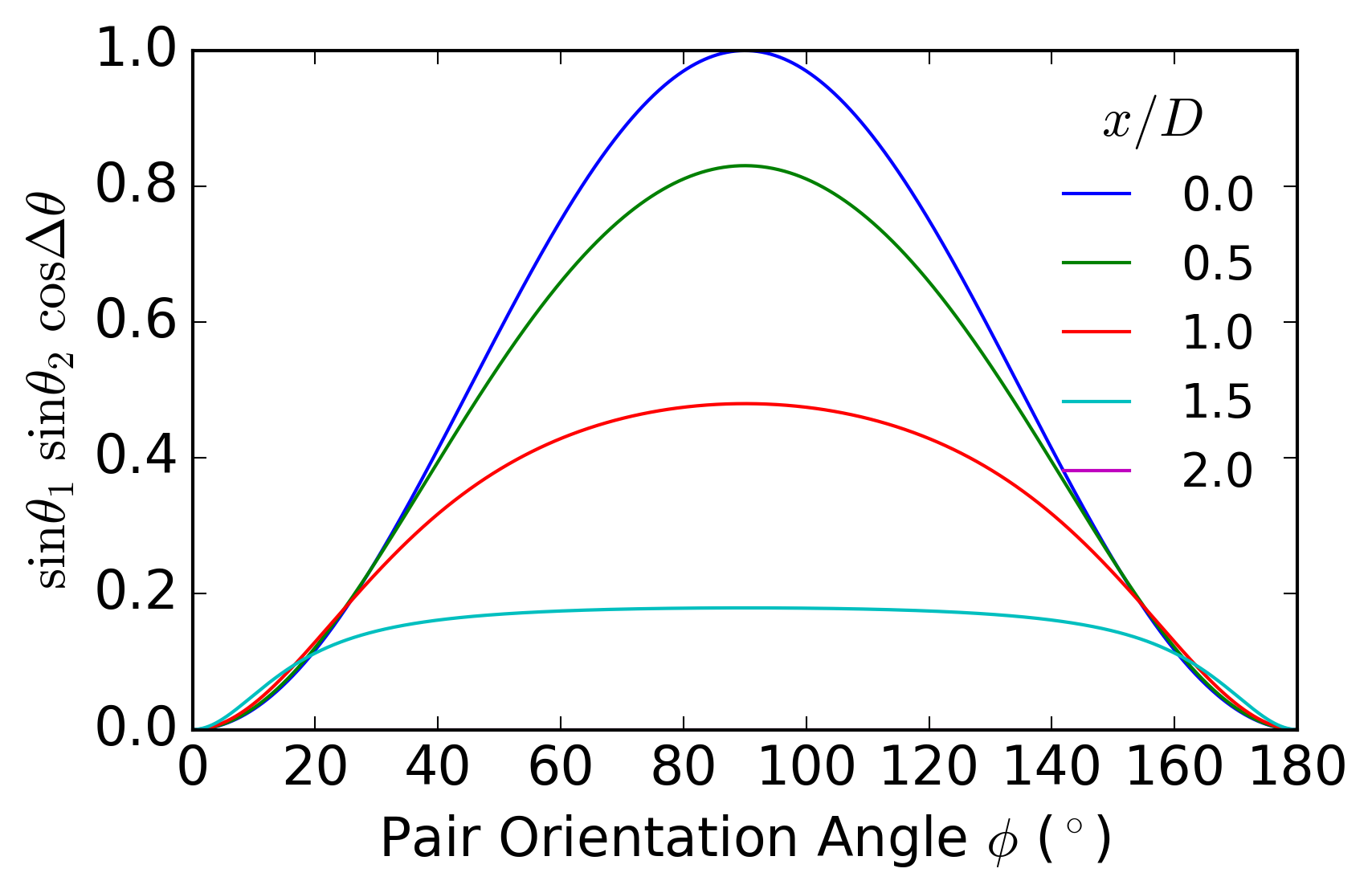
These expressions weight the contributions of the parallel, $\xi_{v,(i)}$ , and perpendicular, $\xi_{v,(iv)}$ , correlation terms to the total correlation $\xi_{v,\perp}$ . Figure 5 plots these angular terms for various $x/D$ and shows that the “parallel” term (left) favors pairs oriented perpendicular to the line of sight (proper motions are along $\hat{x}$ and $\phi=\pi/2$ ) while the “perpendicular” term (right) gives positive weight to pairs oriented roughly $\pm 45^{\circ}$ with respect to the line of sight.

For orientation angle $\phi$ uniformly distributed between 0 and $\pi$ , we integrate Equations 40 and 41 to obtain mean values for these angular weighting terms as a function of $x/D$ . The result predicts the outcome of observations of randomly oriented pairs binned in separation and/or distance. For all but very nearby or large-separation pairs, the orientation-averaged angular terms are insensitive to $x/D$ . For example, the perpendicular angular term’s mean value differs by only $\sim 1\%$ between $x/D=0.2$ and $x/D\rightarrow 0$ . This range will encompass most pairs in a large survey sample.

Figure 6 shows the total transverse peculiar velocity correlation as a function of pair separation for a range of $x/D$ values after averaging over randomly oriented pairs (while keeping pair separation $x$ fixed). This is what one expects to observe using proper motions to calculate the transverse peculiar velocity correlation statistic (Equation 1). The random orientation of pairs dilutes this signal compared to the equidistant pairs case, as expected (Figures 3 and 4), but the correlation function is fairly insensitive to $x/D$ except for very large-separation or nearby pairs (both of which have large angular separations). See Section IV for a parallel treatment of the alternate statistic $\xi^{\prime}_{v,\perp}$ that is substantially less dependent on $x/D$ and shows a larger amplitude.

IV An Alternate Statistic

We define an alternate two-point correlation statistic $\xi^{\prime}_{v,\perp}$ based on the direct (unprojected) inner product of pairs of transverse velocities:

\xi^{\prime}_{v,\perp}(\vec{x}_{1},\vec{x}_{2})\equiv\langle\vec{v}_{\perp}(\vec{x}_{1})\cdot\vec{v}_{\perp}(\vec{x}_{2})\rangle.

(42)

This statistic will produce negative values for pairs of objects that are converging or diverging and positive values for co-streaming motions. Using Equation 5, this becomes

\xi^{\prime}_{v,\perp}(\vec{x}_{1},\vec{x}_{2})=\langle\left[\vec{v}(\vec{x}_{1})-(\vec{v}(\vec{x}_{1})\cdot\hat{x}_{1})\hat{x}_{1}\right]\cdot\left[\vec{v}(\vec{x}_{2})-(\vec{v}(\vec{x}_{2})\cdot\hat{x}_{2})\hat{x}_{2}\right]\rangle.

(43)

This expression expands into four parts that can be treated separately:

	$\displaystyle\xi^{\prime}_{v,\perp}(\vec{x}_{1},\vec{x}_{2})=\langle\overbrace{\vec{v}(\vec{x}_{1})\cdot\vec{v}(\vec{x}_{2})}^{(i)}\rangle+\langle\overbrace{-(\vec{v}(\vec{x}_{1})\cdot\hat{x}_{1})(\vec{v}(\vec{x}_{2})\cdot\hat{x}_{1})}^{(ii)}\rangle+\langle\overbrace{-(\vec{v}(\vec{x}_{2})\cdot\hat{x}_{2})(\vec{v}(\vec{x}_{1})\cdot\hat{x}_{2})}^{(iii)}\rangle$
	$\displaystyle+\langle\overbrace{(\vec{v}(\vec{x}_{1})\cdot\hat{x}_{1})(\vec{v}(\vec{x}_{2})\cdot\hat{x}_{2})\cos\Delta\theta}^{(iv)}\rangle$		(44)

where $\cos\Delta\theta=\hat{x}_{1}\cdot\hat{x}_{2}$ . Following the derivation in Section II.1, we work with the velocities in wavenumber space and relate velocity correlations to the matter power spectrum. For parts $(ii)$ – $(iv)$ , it is straightforward to show that these can be written in terms of the correlation integrals parallel and perpendicular to $\hat{x}$ , $\xi_{v,(i)}(x)$ and $\xi_{v,(iv)}(x)$ , derived in Section II.1:

$\displaystyle(ii)$	$\displaystyle:$	$\displaystyle\ \ \langle-(\vec{v}(\vec{x}_{1})\cdot\hat{x}_{1})(\vec{v}(\vec{x}_{2})\cdot\hat{x}_{1})\rangle=-\sin^{2}\theta_{1}\ \xi_{v,(iv)}(x)-\cos^{2}\theta_{1}\ \xi_{v,(i)}(x)$	(45)
$\displaystyle(iii)$	$\displaystyle:$	$\displaystyle\ \ \langle-(\vec{v}(\vec{x}_{2})\cdot\hat{x}_{2})(\vec{v}(\vec{x}_{1})\cdot\hat{x}_{2})\rangle=-\sin^{2}\theta_{2}\ \xi_{v,(iv)}(x)-\cos^{2}\theta_{2}\ \xi_{v,(i)}(x)$	(46)
$\displaystyle(iv)$	$\displaystyle:$	$\displaystyle\ \ \langle(\vec{v}(\vec{x}_{1})\cdot\hat{x}_{1})(\vec{v}(\vec{x}_{2})\cdot\hat{x}_{2})\cos\Delta\theta\rangle=\cos\Delta\theta\sin\theta_{1}\sin\theta_{2}\ \xi_{v,(iv)}(x)+\cos\Delta\theta\cos\theta_{1}\cos\theta_{2}\ \xi_{v,(i)}(x).$	(47)

Part $(i)$ , however, is slightly different:

$\displaystyle\langle\vec{v}(\vec{x}_{1})\cdot\vec{v}(\vec{x}_{2})\rangle$	$\displaystyle=$	$\displaystyle\int{d^{3}k\over(2\pi)^{3}}\ e^{i\vec{k}\cdot\vec{x}_{1}}\int{d^{3}k^{\prime}\over(2\pi)^{3}}\ e^{-i\vec{k}^{\prime}\cdot\vec{x}_{2}}\ \langle\vec{v}(\vec{k})\cdot\vec{v}^{\,*}(\vec{k}^{\prime})\rangle$	(48)
	$\displaystyle=$	$\displaystyle f^{2}H_{0}^{2}\ \int{d^{3}k\over(2\pi)^{3}}\ e^{i\vec{k}\cdot\vec{x}_{1}}\int{d^{3}k^{\prime}\over(2\pi)^{3}}\ e^{-i\vec{k}^{\prime}\cdot\vec{x}_{2}}\ \langle\delta(\vec{k})\delta^{*}(\vec{k}^{\prime})\rangle{(\vec{k}\cdot\vec{k}^{\prime})\over k^{2}k^{\prime\,2}}$	(49)
	$\displaystyle=$	$\displaystyle f^{2}H_{0}^{2}\ \int_{0}^{\infty}{dk\,k^{2}\over(2\pi)^{3}}\ P(k)\int d\Omega_{k}\ e^{i\vec{k}\cdot\vec{x}}\ {(\vec{k}\cdot\vec{k})\over k^{4}}$	(50)
	$\displaystyle=$	$\displaystyle f^{2}H_{0}^{2}\ \int_{0}^{\infty}{dk\,\over 2\pi^{2}k}\ P(k)\ k\ j_{0}(kx).$	(51)

To recast this result in terms of the previous integration kernels, we can use the identity

j_{0}(kx)=-j^{\prime\prime}_{0}(kx)-2\,{j^{\prime}_{0}(kx)\over kx}

(52)

and obtain a result for part $(i)$ :

(i):\ \ \langle\vec{v}(\vec{x}_{1})\cdot\vec{v}(\vec{x}_{2})\rangle=2\ \xi_{v,(iv)}(x)+\xi_{v,(i)}(x).

(53)

Summing all parts of Equation 44, we have

\xi^{\prime}_{v,\perp}(\vec{x}_{1},\vec{x}_{2})=\sin\theta_{1}\sin\theta_{2}\cos\Delta\theta\ \xi_{v,(i)}(x)+(1+\cos\theta_{1}\cos\theta_{2}\cos\Delta\theta)\ \xi_{v,(iv)}(x)

(54)

	$\displaystyle\xi^{\prime}_{v,\perp}(\vec{x}_{1},\vec{x}_{2})=-f^{2}H_{0}^{2}\left[\sin\theta_{1}\sin\theta_{2}\cos\Delta\theta\ \int_{0}^{\infty}{dk\over 2\pi^{2}k}\ P(k)\ k\ j_{0}^{\prime\prime}(kx)\right.$
	$\displaystyle+\left.(1+\cos\theta_{1}\cos\theta_{2}\cos\Delta\theta)\ \int_{0}^{\infty}{dk\over 2\pi^{2}k}\ P(k)\ {j_{0}^{\prime}(kx)\over x}\right].$		(55)

IV.1 Equidistant Pairs

In the simplified case where the two objects lie at the same distance, Equation 54 becomes

\xi^{\prime}_{v,\perp}(\vec{x}_{1},\vec{x}_{2})\Bigr\rvert_{|\vec{x}_{1}|=|\vec{x}_{2}|}=\cos^{2}{\Delta\theta\over 2}\cos\Delta\theta\ \xi_{v,(i)}(x)+\left(1-\sin^{2}{\Delta\theta\over 2}\cos\Delta\theta\right)\ \xi_{v,(iv)}(x).

(56)

Figure 7 shows the correlation versus pair separation (left) and angular separation (right) in this case. This alternate correlation statistic is remarkably different from the statistic plotted in Figure 3: it is never negative, it is fairly insensitive to angular separation, and $\xi^{\prime}_{v,\perp}$ shows a larger amplitude than $\xi_{v,\perp}$ for all $x$ and $\Delta\theta$ .

Following the treatment in Section III.1, Equation 56 can be rewritten in terms of the ratio of the physical separation of pairs $x$ to the distance to each object ( $x_{1}=|\vec{x}_{1}|=|\vec{x}_{2}|$ ):

\xi^{\prime}_{v,\perp}(\vec{x}_{1},\vec{x}_{2})\Bigr\rvert_{|\vec{x}_{1}|=|\vec{x}_{2}|}=\left[1-3\left({x\over 2x_{1}}\right)^{2}+2\left({x\over 2x_{1}}\right)^{4}\right]\xi_{v,(i)}(x)+\left[1-\left({x\over 2x_{1}}\right)^{2}+2\left({x\over 2x_{1}}\right)^{4}\right]\xi_{v,(iv)}(x).

(57)

When the two objects in a pair are equidistant, the largest possible pair separation is twice the distance to each object ( $\Delta\theta=\pi$ ), and the smallest possible distance to each object is half of the pair separation. When these extremal conditions are met, $\xi^{\prime}_{v,\perp}=2\ \xi_{v,(iv)}$ . On the other hand, when pairs have separations that are small compared to their distance, $\Delta\theta$ is small and the correlation asymptotes to $\xi_{v,(i)}+\xi_{v,(iv)}<2\ \xi_{v,(iv)}$ . Figure 8 (right) demonstrates that for $x_{1}\gtrsim 4x$ , the correlation becomes nearly constant (but is not a maximum). The asymptote for $x_{1}\gtrsim 4x$ has a lower amplitude than the maximal value when $x_{1}=x/2$ .

IV.2 Randomly Oriented Pairs

The angular terms in Equation 54 can be expressed in terms of the pair orientation angle $\phi$ and the separation-to-distance ratio $x/D$ :

	$\displaystyle\sin\theta_{1}\sin\theta_{2}\cos\Delta\theta$	$\displaystyle=$	$\displaystyle{\left(1-{1\over 4}\left(x\over D\right)^{2}\right)\sin^{2}\phi\over 1+\left({x\over D}\right)^{2}\left(\sin^{2}\phi-{1\over 2}\right)+{1\over 16}\left(x\over D\right)^{4}}$		(58)
	$\displaystyle 1+\cos\theta_{1}\cos\theta_{2}\cos\Delta\theta$	$\displaystyle=$	$\displaystyle 2-{\left(1+{3\over 4}\left(x\over D\right)^{2}\right)\sin^{2}\phi\over 1+\left({x\over D}\right)^{2}\left(\sin^{2}\phi-{1\over 2}\right)+{1\over 16}\left(x\over D\right)^{4}}.$		(59)

Figure 9 plots the angular terms versus pair orientation, showing that even for a radially oriented pair ( $\phi=0$ ) this statistic is sensitive to correlated peculiar velocity. For uniformly random orientations, we calculate the mean values for these angular terms and sum the components of Equation 54 to obtain the transverse velocity correlation shown in Figure 10. This alternate statistic is roughly four times larger than the projected statistic and it is insensitive to $x/D$ . This statistic is observation-friendly because one can simply average pair measurements binned by pair separation.

V Discussion

Given the results above, proper motion observations should focus on the smallest physical separation pairs of galaxies or AGN that also have small angular separations (large distances), or small $x/D$ . This strategy will maximize the expected correlation signal. The caveat to this guidance, which suggests that the best tracers of transverse peculiar motions would be distant small-separation pairs of objects, is that the observed quantity is the proper motion. The rest-frame transverse velocity is proportional to the proper motion and the distance,

\vec{v}_{\perp}=D_{M}\ \vec{\mu},

(60)

where $D_{M}$ is the proper motion distance (equivalent to the comoving distance in a flat cosmology and related to the angular diameter distance as $D_{M}=D_{A}(1+z)$ [8]). Uncertainties in proper motion measurements will therefore scale linearly with distance when translated into transverse velocity uncertainties. A typical peculiar velocity of 300 km s^-1 equates to a proper motion of 6.3 $\mu$ as yr^-1 at 10 Mpc. A sample of objects with proper motion uncertainty $\sigma_{\mu}=100$ $\mu$ as yr^-1 would require roughly 250 independent measurements to reach this proper motion value and roughly 2300 measurements to achieve 3 $\sigma$ significance. Such averaging to reduce statistical errors would only be possible if one knew a priori the orientation of each proper motion vector in the sample. Since this is not known, it is appropriate to examine correlation of extragalactic pairs.

Since the number of galaxies in a volume scales as $N\propto D^{3}$ , and the number of possible pairs scales as $N_{p}\sim N^{2}$ , then the number of pairs scales as $N_{p}\propto D^{6}$ . The uncertainty in the transverse velocity correlation scales as $\sigma_{\xi_{\perp}}\propto v_{\perp}\,\sigma_{v_{\perp}}N_{p}^{-1/2}$ . Using Equation 60, and assuming that the fractional proper motion uncertainty is much larger than the distance uncertainty, $\sigma_{v_{\perp}}=\sigma_{\mu}D$ . The uncertainty in the correlation therefore scales roughly as $\sigma_{\xi_{\perp}}\propto\mu\,\sigma_{\mu}D^{-1}$ . This relationship assumes that $x/D\lesssim 1$ , that pairs represent independent measurements of the peculiar velocity field (not strictly true), that the proper motion measurements in value and uncertainty are uniform among the sample, and it neglects the random orientations of pairs. Including these effects will impact the constant of proportionality and may diminish the favorable impact of distance on the uncertainty in the measured correlation statistic.

The optimal strategy for measuring the transverse peculiar velocity created by large scale structure will depend on the data in hand: the redshift distribution, pair separations, sample size, and proper motion precision. VLBI proper motions will likely have redshifts $z\sim 1$ , proper motion uncertainties per object of $\sigma_{\mu}\sim 10$ $\mu$ as yr^-1, and sample size of 500–1000 objects [2, 14, e.g.,]. Gaia AGN proper motions will have lower redshifts, smaller pair separations, and sample size $\sim 10^{5}$ , but larger per-object proper motion uncertainties of $\sim 200$ $\mu$ as yr^-1 [12, 15, e.g.,].

VI Conclusions and Future Work

We have developed two-point transverse peculiar velocity correlation statistics that connect the matter power spectrum to extragalactic proper motions. We have explored the impact of pair separation, distance, and angular separation on these correlations and suggested some strategies for future extragalactic proper motion surveys. Except for very nearby pairs of objects that subtend large angles, close pairs are more sensitive to large scale structure than widely-separated pairs, as one might expect. We develop correlation statistics for randomly oriented pairs of objects with various separation-to-distance ratios. Finally, we suggest that the sensitivity to the transverse velocity correlation improves with distance in volume-limited surveys, but the optimal detection strategy will depend on the nature of the proper motion data in hand.

The work presented here has limitations that point to obvious directions for future work:

•

The two-point correlation statistics presented here are scalars while the inputs are proper motion vectors, so this work is not taking full advantage of the available observational information. We suggest that future work should consider a vector correlation measure. What this might look like, we do not know.
•

It will also be important to extend this work to higher redshifts, which will require modifications to $f$ , $H_{0}$ , and the power spectrum $P(k)$ . The treatment above is correct for low redshift, but quasars in general and radio sources in particular are significantly redshifted, and VLBI or Gaia samples will typically have mean redshifts of $z\sim 1$ , which is much more distant than traditional radial peculiar velocity surveys.
•

Very close pairs of objects will not obey linear perturbation theory. A complete treatment will need to rely on numerical simulations.

Ultimately, it may be possible to combine this work with radial peculiar velocities to obtain a true three-dimensional peculiar velocity map of the local universe.

The authors acknowledge support from the NSF grant AST-1411605 and the NASA grant 14-ATP14-0086. We thank the anonymous referee for helpful suggestions and for calculation validation. We acknowledge the use of the Legacy Archive for Microwave Background Data Analysis (LAMBDA), part of the High Energy Astrophysics Science Archive Center (HEASARC). HEASARC/LAMBDA is a service of the Astrophysics Science Division at the NASA Goddard Space Flight Center.

References

[1] Bower, G. C., Demorest, P., Braatz, J., et al. 2015, Next Generation Very Large Array Memo No. 9 Science Working Group 4, arXiv:1510.06432
[2] Darling, J. 2013, ApJL, 777, L21
[3] Darling, J. 2014, MNRAS, 441, L66
[4] Darling, J., Truebenbach, A. E., & Paine, J. 2018, ApJ, in press (arXiv:1804.06986)
[5] Dekel, A. 1997, “Galaxy Scaling Relations: Origins, Evolution and Applications,” proceedings from the ESO Workshop held November, 1996, eds. L. N. da Costa & A. Renzini (Springer-Verlag), p. 245 (astro-ph/9705033)
[6] Ding, F., & Croft, R. A. C. 2009, MNRAS, 397, 1739
[7] Dodelson, S. 2003, Academic Press.
[8] Hogg, D. W. 1999, astro-ph/9905116
[9] Kochanek, C. S., Kolatt, T. S., & Bartelmann, M. 1996, ApJ, 473, 610
[10] Mediavilla, E., Jiménez-Vicente, J., Muñoz, J. A., Mediavilla, T., & Ariza, O. 2015, ApJ, 798, 138
[11] Mediavilla, E., Jiménez-Vicente, J., Muñoz, J. A., & Battaner, E. 2016, ApJ, 832, 46
[12] Paine, J., Darling, J., & Truebenbach, A. E. 2018, ApJ, in press (arXiv:1804.02064)
[13] Strauss, M. A., & Willick, J. A. 1995, Physics Reports, 261, 271
[14] Truebenbach, A. E. & Darling, J. 2017, ApJS, 233, 3
[15] Truebenbach, A. E. & Darling, J. 2018, ApJ, submitted
[16] Tully, R. B., Courtois, H., Hoffman, Y., & Pomaréde, D. 2014, Nature, 513, 71