Keywords: Hénon map, symplectic maps, saddle-center bifurcation, Krein bifurcation, accelerator modes, invariant tori
Elliptic Bubbles in Moser’s 4D Quadratic Map:
the Quadfurcation
Abstract
Moser derived a normal form for the family of four-dimensional, quadratic, symplectic maps in 1994. This six-parameter family generalizes Hénon’s ubiquitous 2d map and provides a local approximation for the dynamics of more general 4d maps. We show that the bounded dynamics of Moser’s family is organized by a codimension-three bifurcation that creates four fixed points—a bifurcation analogous to a doubled, saddle-center—which we call a quadfurcation.
In some sectors of parameter space a quadfurcation creates four fixed points from none, and in others it is the collision of a pair of fixed points that re-emerge as two or possibly four. In the simplest case the dynamics is similar to the cross product of a pair of Hénon maps, but more typically the stability of the created fixed points does not have this simple form. Up to two of the fixed points can be doubly-elliptic and be surrounded by bubbles of invariant two-tori; these dominate the set of bounded orbits. The quadfurcation can also create one or two complex-unstable (Krein) fixed points.
Special cases of the quadfurcation correspond to a pair of weakly coupled Hénon maps near their saddle-center bifurcations. The quadfurcation also occurs in the creation of accelerator modes in a 4d standard map.
1 Introduction
Multi-dimensional Hamiltonian systems model dynamics on scales ranging from zettameters, for the dynamics of stars in galaxies [1, 2], to nanometers, in atoms and molecules [3, 4]. Hamiltonian flows generate symplectic maps on Poincaré sections [5, §9.14], and numerical algorithms for these flows can be symplectic [6, 7]. Symplectic maps also arise directly in discrete-time models of such phenomena as molecular vibrations [8, 9], stability of particle storage rings [10, 11], heating of particles in plasmas [12], microwave ionization of hydrogen [13] and chaos in celestial mechanics [14]
A map is canonically symplectic for coordinates and momenta if its Jacobian matrix, , satisfies
| (1) |
where is the Poisson matrix. In particular this implies that the map is volume preserving: .
Perhaps the most famous symplectic map is the area-preserving map introduced by Hénon in 1969 as an elemental model to inform his studies of celestial mechanics [15]. This map is also the simplest nonlinear symplectic map, since it contains a single quadratic term, and yet—as Hénon showed—every quadratic area-preserving map can be reduced to his form [16].
Quadratic maps are useful because they model the dynamics of smooth maps in the neighborhood of a fixed point or periodic orbit. For example, quadratic terms in the power series give a local description of the dynamics near an accelerator mode of Chirikov’s standard map [17]. More generally, any symplectic diffeomorphism can be approximated by a polynomial map on a compact set [18].
Higher-dimensional analogues of Hénon’s map were proposed in [19], and similar maps were used to study the stickiness of regions near an elliptic fixed point [20], the resonant formation of periodic orbits and invariant circles [21, 22, 23, 24], bifurcations due to twist singularities [25], and the dynamics near a homoclinic orbit to a saddle-center fixed point [26]. Such maps model a focussing-defocussing (FODO) magnet cell in a particle accelerator and have been used to study the structure of bounded orbits, the dynamic aperture, and robustness of invariant tori [27, 28, 29, 30].
In 1994, Moser [31] showed that every quadratic symplectic map on is conjugate to the form
| (2) |
Here are symplectic maps, is linear and is affine, and is a symplectic shear:
| (3) |
where is a cubic potential. There are several immediate consequences of this representation. Firstly, if the quadratic map has finitely many fixed points, as it generically will, then there are at most [31]. Note that more generally a quadratic non-symplectic map on a -dimensional space could have as many as isolated fixed points. Secondly, since the inverse of is also a quadratic shear of the same form (replace by ), the inverse of any quadratic, symplectic map is also quadratic. More generally, the inverse of a quadratic diffeomorphism could be a polynomial map of higher degree [32, Thm 1.5]; for example, the inverse of the volume-preserving map has degree eight. The form (2) also applies to cubic maps, but not to higher degree polynomial maps [33].
In this paper we study the dynamics of Moser’s map in four dimensions. The normal form for the 4d case is reviewed and slightly transformed for convenience in §2. We argue in §3 that its fixed points are most properly viewed as arising from a bifurcation in which they emerge from a single fixed point as parameters are varied away from a codimension-three surface. Since this bifurcation often results in the creation of four fixed points, we call it a quadfurcation, with thanks to Strogatz who, “with tongue in cheek,” proposed the term in an exercise for 1d odes in his well-known textbook [34, Ex. 3.4.12].
As we will see in §3.1, the unfolding of the quadfurcation in Moser’s map can lead to (i) the creation of four fixed points from none, or (ii) a collision and re-emergence of two pairs of fixed points, or (iii) even the collision of a pair leading to four fixed points. The stability of these fixed points is investigated in §3.2. The unfolding of the quadfurcation along paths in parameter space is studied in §3.3-§3.4. When the map is reversible, §3.5, additional cases occur including the simplest one: the Cartesian product of a pair of area-preserving maps. We investigate the creation of families of invariant two-tori, as expected from KAM theory, around doubly elliptic fixed points in §3.6. In §3.7 we observe that these bubbles of elliptic orbits strongly correlate with the regions of bounded dynamics.
Since Moser’s map is affinely conjugate to the general quadratic, symplectic map, it must have a limit in which it reduces to a pair of uncoupled Hénon maps—we show this in §4. Finally, we show in §5 that the dynamics near an accelerator mode of the 4d standard map (Froeschlé’s map [35]), can be modeled by Moser’s map, and indeed, the local dynamics reduces to a coupled version of the Hénon maps obtained in the previous section.
2 Moser’s quadratic, symplectic map
2.1 Four-Dimensional Normal Form
For the two-dimensional case, the map (2) can be transformed by an affine coordinate change to the Hénon map ,
| (4) |
with a single parameter . When this map has an elliptic fixed point (for ), it is conjugate to the map whose dynamics were first studied by Hénon [15]. By a similar transformation Moser showed [31] that in four dimensions, (2) can generically be written as
| (5) |
where
| (6) | ||||
and , . Here there are two discrete parameters, , and or . The remaining six parameters are free. It is convenient to think of the six real parameters of as and , where
| (7) |
Indeed, given these six, and the sign , we can determine the off-diagonal elements of from
| (8) |
The choice of the sign here is unimportant since this simply replaces with , and the resulting map is conjugate to the inverse of (5); see §2.3. Note that (8) has real solutions only when , and that is symmetric only at the lower bound of this inequality.
2.2 Shifted Coordinates
As a first step in the analysis of the dynamics of (5), we will study its fixed points. To do this it is convenient to define shifted variables and parameters. There is a codimension-three set of parameters where the map has exactly one fixed point, and focussing on this set simplifies the calculations more generally.
For any matrix and when , the map (5) has exactly one fixed point at
| (9) | ||||
when the parameters of the potential (6) take the values
| (10) | ||||
To see this, and to simplify the computations it is convenient to shift coordinates so that the origin is at the point and to define new shifted parameters:
| (11) | ||||
In these new coordinates, (5) becomes
| (12) |
where the new potential,
| (13) |
is the same as from (6) upon replacing by . This shifted form of Moser’s quadratic, symplectic map is convenient because several computations can be carried out more easily and many of the expressions we obtain below will be more compact.
The map (12) is generated by the discrete Lagrangian
| (14) |
through the equation
In other words the map is implicitly defined by and . This means that is exact symplectic [36], and of course, that it preserves the symplectic form . Note also that if we denote an orbit of (12) as a sequence
| (15) |
and define the action of a finite portion by
then each stationary point of , for fixed endpoints, is a segment of an orbit with the momentum determined by .
2.3 Second Difference Form and ODE Limit
The shifted form (12) of Moser’s map can be written as a second difference equation. Denoting an orbit as (15), then and the map (12) is equivalent to
| (16) |
One immediate consequence of (16) is that the replacement is clearly equivalent to inverting the map. Therefore the invariant sets of the Moser map with are the same as those of the original map. Similarly, note that the replacement together with and leaves the Moser map invariant. We will also use the form (16) in §3.2 and §3.7.
To emphasize the different roles of the symmetric and antisymmetric parts of , let
| (17) | ||||
where and, as before . Then (16) becomes
| (18) |
In this form the map closely resembles a pair of second order differential equations.
Indeed in a neighborhood of the origin in the phase space, , and in the space of the new parameters, , (18) approaches a Lagrangian system of ODEs. To see this, formally introduce a parameter , and scale
Here represents the deviation from symmetry, so that . Then in the limit , the second difference equation (16) limits on a system of ODEs in a scaled time , and a new variable
This scaling implies that for the potential (13), . Moreover, as , the second difference and the first difference . Substituting these into (18), gives the limiting system
| (19) |
as . Thus the symmetric part of corresponds to a mass matrix, multiplying the acceleration. By contrast, corresponds to a Coriolis-like force, which is proportional to the velocity.
The system (19) is obtained from the Lagrangian
| (20) |
To convert (19) into a Hamiltonian system define the canonical momenta
giving a Hamiltonian, , that has Coriolis and centripetal terms:
| (21) |
Thus is the mass matrix, and is the negative of the potential energy. The antisymmetric matrix contributes both a Coriolis-like term, bilinear in and , and a centripetal-like term, quadratic in . We will use this interpretation, for the case of symmetric , in §3.5.
3 Quadfurcation
From the general theory [31] we know that (5) and hence (12) has at most four (isolated) fixed points. On the codimension-three surface in parameter space there is a single fixed point (unless ). As we will see below, there are sectors in parameter space near this surface for which there are no fixed points, and sectors for which there are four. It seems appropriate to call the creation of four fixed points from none a quadfurcation. In some cases a quadfurcation can be analogous to a simultaneous pair of co-located saddle-center bifurcations; however, the stabilities of the resulting fixed points are usually not those of a pair of decoupled area-preserving maps, namely the Cartesian product of 2d saddles and centers.
In the following subsections we study the fixed points, their stability, and the structure of the region of phase space around the elliptic fixed points that contains bounded orbits.
3.1 Fixed Points
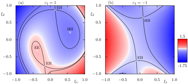
The coordinates, , of the fixed points of (12) are critical points of the cubic polynomial (13). Several contour plots of are shown in Fig. 1. Critical points satisfy the equations
| (22) |
Note that the positions are independent of the matrix , though the momenta, determined by , depend on the full matrix. Note that if for parameters , then it is also zero at the point for parameters and at the point for . Thus we can restrict attention to .
The case is an organizing center for the solutions of (22). In this case the second component immediately implies that either or . Then, whenever , the first implies that both . We call this the quadfurcation point. Since the matrix elements are still free parameters, it occurs on a codimension-three surface in the six-dimensional parameter space. The off-diagonal elements of the matrix, and , are then fixed up to exchange by the condition det, (8). In the parameterization (12) the quadfurcation surface is just the three-plane . In Moser’s original parameterization, this surface is determined by (10).

More generally if then (22) implies that , so
| (23) |
Substituting into the first component of (22) then shows that must be a root of the scalar polynomial
| (24) |
When this polynomial is quartic, and so has at most four roots. Since has no linear term, it has exactly one root in only when , on the quadfurcation set. When , is at most cubic, and there are at most three isolated roots. Several examples are shown in Fig. 2.
There are various regions in the parameter space that have different numbers of fixed points. We now determine the bifurcation sets, which separate these regions: to find these sets when , it is easiest to solve for the surfaces on which there are double roots, i.e., and . First, always has a critical point, , at , and it has two more critical points if
| (25) |
Eliminating from the two equations gives the discriminant
Thus there are double roots at , and on the surfaces , where
| (26) |
For these surfaces to be real, the radical in (26) must be real, i.e., (25) must be satisfied. Moreover letting
| (27) |
then and . To define real-valued functions let
| (28) | ||||
The resulting surfaces are shown in Fig. 3.


If , then when there are no real roots. At the upper surface, , which is nonzero for , two roots are created. Two additional roots are created upon crossing , which is nonzero for , see Table 1. The two surfaces intersect at on the line . Crossing this codimension-two set at and moving into the region thus corresponds to the simultaneous creation of four fixed points at two different locations, i.e., to a pair of simultaneous saddle-center bifurcations, as we will see in §3.2.
If , then (24) has four real roots only if and . Note that is nonzero only when . Inside cusp-like shape formed from the surfaces, as shown in Fig. 3(b), there are four roots. Going outwards from this region, by either crossing or , two solutions disappear in a saddle-center bifurcation. Thus on the surfaces or there are three roots (one of them with multiplicity 2). When these surfaces merge, on the curve and , there are two fixed points:
The cases and require special treatment. When but , the polynomial (24) has no cubic term and the fixed points can be solved for explicitly:
| (29) |
where is then obtained from (23). Note that there are four possible points here, with choices for the outer and the inner . This equation gives real solutions only when both square roots are real. When , (29) gives four real solutions if . On the boundary , these four solutions are created in two pairs, at
These pairs merge at the quadfurcation point . If then only the inner sign choice is valid and (29) gives two real solutions whenever or . Table 1 delineates the possibilities.
If , then (22) implies that either or . The first component of (22) is then trivially a quadratic. In this case the four solutions are
| (30) |
Note that when there are four real fixed points whenever , and two in the range . If , then the first pair is real when , and the second pair is real only if . Thus there are four real fixed points when .
| Number of Fixed Points | |||||||
| 1 | |||||||
| , | , | , | |||||
| or | or | and | |||||
| always | |||||||
| 0 | |||||||
For and , the polynomial (24) is cubic, so there is always at least one fixed point. The critical points of are at and , and critical values and . Thus there are three fixed points when
| (31) |
If , then the polynomial (24) is at most quadratic. It has two solutions if . Special cases are again shown in Table 1. Finally, when , there is a line of fixed points at . This case (not shown in Table 1) is the only one for which there are infinitely many fixed points.
3.2 Stability
The stability properties of fixed points of the map (12) are most easily computed using the second difference form (16). Linearization about a fixed point gives the eigenvalue problem
| (32) |
where is the symmetric matrix
| (33) |
Given the coordinate eigenvector , the momentum components are . A similar analysis can be used, more generally, for a period- orbit, see [37, eqs. (21)-(22)].
Thus for a nontrivial solution of (32), the matrix
must be singular. Since the map is symplectic its eigenvalues must satisfy the reflexive property: if is an eigenvalue, then so is . This follows for (32) because implies that . As a consequence the characteristic polynomial can be written as a quadratic in the partial trace :
| (34) |
where we recall that . The parameters are Broucke’s stability parameters [38, 39]. More generally, these parameters are determined by the linearized map at a fixed point, by and ; equivalently, in terms of the eigenvalues of the reduced characteristic polynomial one has and , or explicitly
| (35) |
where are the two reciprocal pairs of eigenvalues of the characteristic polynomial of the linearized map.
The -plane is divided into seven stability regions as shown in Fig. 4. These are bounded by the saddle-center (), and period-doubling () lines:
| (36) | ||||
on which there is a pair of eigenvalues at or , respectively, and the Krein parabola ()
| (37) |
on which there are double eigenvalues on the unit circle (for and ) or real axis (for and .). The point corresponds to four unit eigenvalues. The seven stability regions with different types of linearized dynamics around the fixed point are labeled by combinations of E (elliptic), H (hyperbolic), and I (inverse hyperbolic), each involving a pair of eigenvalues , and in the CU (complex unstable) region, where , there is a complex quartet of eigenvalues.
For a general symmetric , the stability parameters are
For the matrix (33) these become
| (38) | ||||
and the saddle-center and period-doubling parameters are
| (39) | ||||
In particular, note that the sign of depends on the fixed points only through the sign of the Hessian of the potential (13); for example, if , then at extrema and at saddle points of . Finally, the Krein parameter is
| (40) | ||||
At the quadfurcation, where , (38) gives
| (41) | ||||
This implies that the quadfurcation point lies on the saddle-center line; indeed from (39), at this point. When (), then lies below and to the left of (above and to the right of) the point . The quadfurcation occurs at only when , i.e., when the matrix is symmetric, see the discussion in §3.5 below. The quadfurcation occurs below the period-doubling line, i.e., for , only if and .
More generally, since fixed points are critical points of , (22), they can be created or destroyed only when , which is equivalent to by (39). This can also be seen upon computing the resultant of and (24)—recall that the resultant gives the set of parameters on which two polynomials simultaneously vanish. This resultant is proportional to . Of course, this is what we saw in Fig. 3—pairs of fixed points are created or destroyed upon crossing the surfaces (28).
3.3 Quadfurcation along a Line in Parameter Space
Near the quadfurcation, if we assume that for , then , the cubic term involving in (24) is negligible to lowest order, and the fixed points are given by (29) to . Substitution into the stability criteria then gives
| (42a) | ||||
| (42b) | ||||
| (42c) | ||||
Note that the signs in (42a) correspond to the inner in (29), the sign inside the square root. Using these results, we can get an overview of all possible stability scenarios of the fixed points created in a quadfurcation, see Table 2 and Fig. 5. As the quadfurcation point shifts along the line, different stabilities occur, but since and generically , the branches emerge tangentially to the line (the term could vanish, but this is exceptional). Moreover, the sign of depends on the choice of the outer sign in (29), so this pair of fixed points form a parabolic curve that is tangent to the line at the quadfurcation point.
| Condition | Fixed Points and Stability | |||
|---|---|---|---|---|
| on | , | , or | ||
| 2 EH 2 HH | 2 HH | |||
| see §3.5 | see §3.5 | |||
| 2 EE 2 EH | 2 EH | |||
| IE EE IH EH | IH EH | |||
| 2 IE 2 IH | 2 IH | |||
Finally, note that when , then at the quadfurcation, and hence a direct transition to the complex unstable (CU) region is only possible in the symmetric case for which ; this is discussed in §3.5.
For the basic structure is the one shown in the fourth column of Table 2 and Fig. 5(a, c): four new branches emerge from a point on the saddle-center line. In each case, two of the fixed points are above (), and two are below (), this line. The implication is that when , and the quadfurcation occurs below the line and corresponds to the transition
i.e., two of the created fixed points are of type IE and two of type IH (this is not shown in Fig. 5, but compare with Fig. 4). Perhaps the most interesting quadfurcation creates stable fixed points. This occurs for and , where we have the transition
| (43) |
This is the case shown in Fig. 5(a): as decreases from zero, the two created EE points move along the green and black curves in the figure and the two EH points move along the red and blue curves.
Note that one of the EE points in this figure eventually undergoes a Krein bifurcation, moving into the CU region. The implication is that the Krein signature of this point must have been indefinite when it was created in the quadfurcation, since this signature is constant under parameter variations so long as the stability remains in the interior of the EE-region in Fig. 4 [39, Sec. III].
Finally, when the quadfurcation point is above whenever , so the transition is
| (44) |
This case is shown in Fig. 5(c). Again, a Krein bifurcation, HH CU, eventually occurs.
For the basic structure is shown in the last column of Table 2 and in Fig. 5(b, d). There are two fixed points before and after the quadfurcation with positions given by the inner sign in (29). Using this and (23), there is no sign choice that smoothly connects the branches for to : the fixed points lose their identity when they collide. The sign choice implies that . When , and hence , the fixed points both before and after the quadfurcation are below the line, so the transition is
| (45) |
if . As shown in Fig. 5(b), the fixed points move in towards the line (black and red curves) as colliding at , and splitting apart again for . Similarly, when the transition corresponds to
Finally, when and , the transition is
| (46) |
as shown in Fig. 5(d).
It is interesting that all of this structure is quite different from what would be expected from a pair of decoupled, area-preserving maps undergoing saddle-center bifurcations, where there can be at most one EE point. This case corresponds to the special point , which will be treated in §3.5 and applied to the case of decoupled maps in §4.
3.4 Two to Four Fixed Point Transitions
When a parameter path crosses one of the surfaces then in (39), and the resulting saddle-center bifurcation typically creates or annihilates a pair of new fixed points, one with E eigenvalues and one with H eigenvalues. When , there are two fixed points outside the wedge between and shown in Fig. 3(b), and so if the parameter path enters the wedge then two new fixed points are created. If the path enters the wedge at the quadfurcation point , then the two existing fixed points merge, and the bifurcation—now a quadfurcation—occurs at the origin. Depending upon and the sign , the quadfurcation can occur at any point along the line, and so a number of different stability cases can arise.

An example is shown in Fig. 6 for the parabolic path
| (47) |
as varies, with the remaining parameters as shown in the caption. Figure 6 shows the contours of the potential for , and and Fig. 7 shows the corresponding stability diagram. There are two fixed points when both of type EH; these merge at . The quadfurcation corresponds to a transition
Effectively the original EH pair is reformed and the contour lines near the new EE–EH pair in Fig. 6(c) resemble those for a local saddle-center bifurcation.
3.5 Krein Collisions, Symmetric and Reversibility
As we noted in (41), the quadfurcation occurs for a multiplicity four unit eigenvalue only when the matrix of (6) is symmetric. This is the only case in which the quadfurcation can immediately create fixed points of type CU, recall Fig. 4.
As discussed in §2.3 the inverse of the Moser map is conjugate to the original map upon the replacement . Therefore, when is symmetric, the map (5) is reversible, i.e., it is conjugate to its inverse [40]: for a homeomorphism . For example, the Hénon map (4) is reversible with . In general, the inverse of (12) is
This map is conjugate to when using the reversor
Thus, as Moser showed [31], if is symmetric the map (5), or equivalently (12), is reversible; we do not know if the converse of this statement is true. This reversor is an involution with the fixed set , a 2d plane. All of the fixed points are thus symmetric.
The quadfurcation is especially interesting in the reversible case since, by (38) and (42), only then does it occur for the stability parameters . Indeed as in §3.3, assuming that and near the quadfurcation, the Krein criterion (42c) is zero to , and the first nonzero terms are
where is given by (29). The sign of this parameter can change, depending upon the details. However, note that since depends only on , it does not depend upon the outer sign in (29). Thus when , the fixed points come in pairs with the same sign of .
When , the four created fixed points come in pairs with opposite signs of from (42a). Thus there will be a pair of fixed points of type EH. Since the curves generically emerge tangent to the the line, the second pair will both have type CU or one will be EE and the other HH. For example, a quadfurcation of the form
| (48) |
is shown in Fig. 8(a). For this case to lowest order, where the sign is the inner sign in (29), implying that the two fixed points with the sign have when near the quadfurcation and are thus of type CU. In contrast, for the example shown in Fig. 8(b) the quadfurcation is
| (49) |
as here when the fixed points exist, . This last case is what would happen in a pair of uncoupled 2d maps, and will be seen below in §4.
As in §3.3, when , the quadfurcation at corresponds to a collision and re-emergence of a pair of fixed points with . When , all of the fixed points will have stability type EH, and so the transition will be
and thus follows the pattern shown in Fig. 5(b).
However, when , then implying that EE, HH and CU are all possible. However, since the two fixed points have the inner sign in (29) they will have the same sign of , so we either have a CU pair or an EE+HH pair. The possible transitions are
| (50) |
for which the stability diagram is shown in Fig. 9(a)
| (51) |
with stability diagram shown in in Fig. 9(b) and
| (52) |
with stability diagram shown in Fig. 9(c).
Another technique for analyzing stability in the neighborhood of the quadfurcation is to use the ODE limit (19) with the Hamiltonian (21). Recall that this limit assumes that we assume the scaling , for . This scaling differs from the -scaling by allowing larger relative values for . The implication of this is that the term in , which was negligible when , is formally important when we take . When is symmetric, , and the Coriolis and centripetal-like terms vanish, simply giving
| (53) |
When is positive or negative definite, then the stability is governed entirely by the classification of the critical point of . In particular if then since the potential in (21) is , a minimum of is an HH point, and a maximum is an EE point. Saddles, correspond to EH points. When , the minima are HH and the maxima are EE. This is consistent more generally with (39), which shows that . Two example contour plots for are shown in Fig. 10.
3.6 Elliptic Bubbles
To visualize the dynamics near the fixed points of the 4d map we use a 3d phase space slice [41]. In its simplest form one considers a thickened 3d hyperplane in the 4d phase space defined by fixing one of the coordinates, e.g., , to define the slice of thickness by
Whenever the points of an orbit lie within the slice, the remaining coordinates are displayed in a 3d plot. The parameter determines the resolution of the resulting plot; decreasing requires the computation of longer trajectories as the slice condition is fulfilled less often, but the resulting intersections will be more precise. For example, if a two-torus intersects the hyperplane, it will typically do so in one or more loops. As grows these loops thicken into annuli in the slice. For further examples and detailed discussion see [41, 42, 43, 44, 45, 46].

For our purposes a slightly more general, rotated slice, defined so as to contain all of the fixed points, will be more convenient. Because the momenta of the fixed points are determined by the coordinates through , all fixed points of the 4d map (12) are contained in a 2d plane. Following the ideas of [41, App. 3], we define new coordinates , with , so that the fixed points lie in the two-plane . Thus we define the 3d slice
so that we get as 3d coordinates. Equivalently, this corresponds to using non-orthogonal basis vectors given as columns of the block matrix
As these are linearly independent, they can be used to express any point as linear combination with coefficients . These coefficients can be computed from the scalar products with the dual basis vectors , which are the columns of
Figure 11 shows an example of a slice for the map (12) with the parameters of Fig. 5(a) when . For these parameters the quadfurcation has created two EE and two EH fixed points that, by construction of the 3d slice, lie in the 2d plane . As expected from KAM theory, the EE fixed points should be surrounded by a Cantor family of two-tori on which the dynamics is conjugate to incommensurate rotation. By analogy with Moser’s theorem for 2d maps [47], the density of these tori should approach one as they limit on the EE points providing that the linearized frequencies are not in a low-order resonance. Indeed, the formal normal form expansion around a nonresonant EE point is an integrable twist map to all orders [21], and higher-dimensional results along the lines of Moser’s twist theorem have been proven for elliptic equilibria of Hamiltonian flows [48, 49]. In the 3d slice each of these tori becomes two (or more) thin annular rings, which, since we have set , appear as 1d loops in the figure [41].
This family of two-tori appears to approximately be limited by the locations of the EH fixed points. Indeed, since the center-stable and center-unstable manifolds of the EH points are 3d, they should form boundaries for the elliptic dynamics. Of course, we expect there will be chaotic orbits near these manifolds, and so the regular 2d tori will not extend into the chaotic zone. The black loops in the plot are a selection of 2d tori that are close to the boundary of the regular region. Also shown in the plot is the full orbit of one of these 2d tori, now projected onto the slice; the projected coordinate is encoded in color as indicated in the color bar at the right [50].

Figure 12 shows an example of a slice for the transition (51), when the matrix is symmetric; the parameters correspond to Fig. 9(b) with , close to the quadfurcation. For this case there are only two fixed points, one of type EE and the other of type HH. Here again we see a family of 2d tori surrounding the EE point. This family has a larger extent in the direction than in , and the loops shrink in size as they become closer to the HH point. Note that now the stable and unstable manifolds of the HH point are two-dimensional, and so do not form barriers in 4d.
3.7 Bounded Orbits
Moser showed, under a nondegeneracy condition on the quadratic terms, that the domain of the quadratic map containing bounded orbits is itself bounded [31]. To obtain an explicit bound we consider the second-difference form (16), rewriting it as
| (54) |
where is a constant vector and the linear and quadratic terms are
Using this form we can prove the following.
Theorem 1.
When , all bounded orbits of the map (54) are contained in the disk , where
| (55) |
with for and for , and we define
| (56) | ||||
Proof.
When the norm of the quadratic terms has the lower bound
where we denote .
Using the triangle inequality on (54) gives
| (57) |
Define so that
For example we can use the Frobenius norms of these matrices to give (56) (or the operator norm, in terms of the singular values). Putting the bounds into (57) gives
| (58) |
Let be chosen such that whenever , then . Solving this quadratic, as an equality, gives (55). Using this in (58) implies that whenever ,
| (59) |
Now there are two possible cases:
- •
- •
Alternatively, suppose that . Again, by (59) whenever we have . Thus the sequence strictly increases as decreases. Again, this implies that is unbounded, now as .
Together, these imply the theorem when .
If , then we can see that , indeed
Thus the analysis above works, if we replace by the larger solution to
with , giving (55) again. ∎
Note that if , then
which does not obey a bound of the form needed in the proof of Th. 1. Thus the theorem does not apply to this case. Indeed, we showed in §3.1 that if , then when there is a line of fixed points, recall the discussion in §3.1.
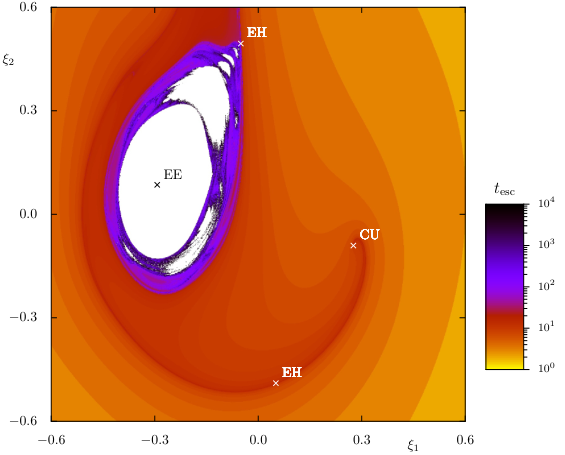
A good way to visualize the distinction between bounded and unbounded orbits for a given parameter set is an escape time plot, see Fig. 13. In this plot, a grid of initial points of the form are iterated until and the required time to escape is encoded in color. Points that have not escaped within iterations are displayed in white. Some of these points lie on a family of regular 2d tori in the neighborhood of the EE fixed point; these will never escape. Points near the boundary of the white region may eventually escape, and indeed, even arbitrarily close to an EE fixed point there are initial conditions that are expected to escape for extremely large times by means of Arnold’s exponentially-slow diffusion mechanism [51, 52, 53, 54].
We can quantify the size of the region of “bounded orbits” under parameter variation by computing the area of the white region in a 2d-plane of initial conditions like that in Fig. 13. For this we choose initial conditions in the two-plane , with varied on a grid of points within the box , and iterate at most steps. Orbits that remain within the disk are counted, and the resulting area is denoted . This area varies as fixed points undergo various bifurcations. A 1d cut through parameter space, Fig. 14, shows how varies with the parameter (here ). Insets in the figure show escape time plots, like that in Fig. 13, for some selected parameters. There is a strong correlation of the area with the structure of the region of stable orbits around the EE point, as we discuss further below.

In Fig. 15 we show as a function of the two parameters and , setting . Note that there are apparently no bounded orbits when (28), where there are no fixed points, nor when or . The largest bounded area occurs in the region near the origin in the plane; recall that the origin corresponds to the quadfurcation since . The dotted curve corresponds to parameters for which , the period-doubling bifurcation (42b). To the left of the curve, the EE fixed point becomes IE and decreases quickly to 0. To the right of the curve and for , the four fixed points have the stabilities EE, EH, EH, and CU. On the curve the EH and CU fixed points coalesce; however, since there are no bounded, regular orbits in a neighborhood these fixed points, this transition does not influence .

At several places in Fig. 14 and along several curves in Fig. 15 one observes a substantial decrease in the bounded area. Several of these can be related to those parameters for which the linearization about the elliptic-elliptic fixed point fulfills a low-order resonance. For such a point the four eigenvalues have the form , and the conjugate/inverse values . Each frequency, , describes the rate of rotation around the fixed point in the 2d invariant planes spanned by the eigenvectors of the corresponding conjugate pair of eigenvalues. These can be written in terms of the partial traces, , recall (35), as
The frequencies of an EE fixed point fulfill a resonance condition when
| (60) |
Without loss of generality, we can set , and . We refer to such a resonance as an resonance.
While resonances are dense in frequency space, those with small order, , are of particular relevance. For example the large white region in Fig. 15 starting for at corresponds to the resonance. This is also manifested in the broad minimum with in Fig. 14. The other prominent minimum near is caused by the resonance. In these two cases is reduced for parameters near those fulfilling the resonance condition. For other indicated resonances, i.e., , and , the density is only reduced on one side of the bifurcation. In the examples this happens for smaller , and sometimes—as for the resonance—it occurs quite some distance away.
Higher order resonances, , should be less important in changing . The results of [21] lead to the expectation that the EE point remains stable, and that for a single resonance the bifurcation creates a pair of invariant 1d tori, one normally hyperbolic and one normally elliptic (at least in the normal form). Further away from the bifurcation of the EE fixed point the geometry is described by bifurcations of families of 1d tori, see [43] and references therein. When the frequency passes through a double resonance, so that are rational, then one expects four periodic orbits to be created [21, 55]. According to [21] their stability is either EE 2 EH HH or 2 EH 2 CU, see [42] for an illustration of the geometry in the first case.

Two further examples of are shown in Fig. 16 with the same parameters as in Fig. 15, except for Fig. 16(a) and for Fig. 16(b) the parameter is fixed. In the latter case the parameter plane no longer intersects the quadfurcation point (), so that the curves do not intersect at the origin in the figure. In Fig. 16(a) the line corresponds to the one in Fig. 15 so that the same resonances are still relevant. These now extend to the region , bending strongly to the right. The same overall resonance structure is also visible in Fig. 16(b).
4 Coupled Hénon Maps
Since Moser’s map, (5) or equivalently (12), is the generic, four-dimensional quadratic map, there must be parameters for which it corresponds to a pair of uncoupled quadratic maps. In this section, we show that this is possible for and special choices of the matrix , depending on . The sign corresponds to positive and negative Krein signatures. These Hénon maps are uncoupled when , but when is nonzero the resulting coupling is, as we will see in §5, precisely what is needed to describe the dynamics in the neighborhood of an accelerator mode of a 4d standard map. Whether there are other possibilities for which the Moser map has uncoupled dynamics with respect to some invariant canonical planes on which the dynamics is conjugate to Hénon maps is presently not clear and left for future study.
Dynamics of a pair of coupled Hénon maps has been studied previously for example in [19, 20, 21, 27, 22, 23, 24, 28, 29, 30], particularly in regard to models of storage rings for particle accelerators.
4.1 Decoupled Limits: Hénon Maps
To find parameter values for which the Moser map is decoupled, we search for a coordinate transformation that reveals the invariant planes. This transformation should be affine in order to maintain the quadratic form. So that the resulting map is symplectic with the standard Poisson matrix (1) and to maintain the momentum-coordinate split for the Hénon form, we start with the linear transformation:
where is invertible and . This transformation is symplectic-with-multiplier, . In the new coordinates the map (12) becomes
where
so that . In order that the map be decoupled in the new coordinates, any cross terms in the new potential should be zero. This can be accomplished for (13) only if , , and is proportional to a rotation by angle . We can normalize the amplitude of the quadratic terms in the new map by setting choosing
to give
The transformation is thus fixed by this choice. In order that the resulting map be decoupled, must be diagonal, e.g.,
| (61) |
where . In order for this to be the case, the original must take one of two forms:
| (62a) | ||||
| (62b) | ||||
Note that one could also replace by in (61), but by the symmetries discussed in §2.3, this gives nothing new.
With this we get the transformed map
This is not quite in the Hénon form (4), but a final affine transformation and brings the map to the form
| (63) | ||||
Note that after this transformation we obtain, when , a pair of uncoupled maps of the Hénon-form (4). However, when , the first canonical pair has the Hénon form only upon a mirroring transformation, e.g., ; the point is that in the canonical coordinates, the components “rotate” under the map in the opposite sense from .
The component maps have saddle-center bifurcations along the lines , creating pairs of fixed points for each component when , respectively. However, in order that the 4d map have a fixed point, both components must have fixed points, implying that . This bifurcation occurs on the same line that appear in Fig. 3(a) when .
When the maps are decoupled, and the four newly created fixed points have types EE, EH, EH and HH. In particular the EE point is located at
In the original variables, the fixed points of these maps are given by (29) since this corresponds to . The doubly elliptic fixed point remains stable in the rectangle
since the individual maps have period-doubling bifurcations at , respectively.
Recall that for a symplectic map (1), with a doubly elliptic fixed point , the quadratic form is an invariant of the linearized dynamics. This implies stability when the form is definite [56, 39]: an EE fixed point cannot cross the line in Fig. 4 into the CU region. Equivalently, the Krein bifurcation cannot occur if the symmetric matrix
is definite. At an elliptic-elliptic point for (63), becomes
where is given in (61). When (63) has an EE point then . This implies that is positive definite when , but has a pair of negative eigenvalues when . Thus, only in the latter case, can coupling lead to a Krein bifurcation.
Indeed, we can see this if we re-introduce coupling by allowing . The same transformations that lead to (63) can be applied if we still take and to be one of the matrices (62). The result is the pair of coupled Hénon maps
| (64) | ||||
where
| (65) | ||||
The stability of the fixed points for this map can be conveniently obtained from the results for the Moser map (12). For and the diagonal matrix in (62a), the stability parameters (38) become
Since the quadfurcation occurs for , , it always occurs at the point for this , as more generally true for the symmetric case in §3.5. For this case the Krein parameter (40) is always nonpositive:
| (66) |
even when the maps are coupled again by nonzero . This reflects the fact that for the two 2d uncoupled maps the elliptic motions in and have the the same orientation. This is not changed by the coupling when , and a CU instability is not possible. This case corresponds to the transition (49) with a stability diagram like that shown in Fig. 8(b) and neither the EE nor the HH fixed point may turn CU.
For the case , and , for the matrix in (62b), we similarly obtain
Now the Krein parameter becomes
| (67) |
which potentially may have either sign. So when the rotation directions for the two canonical planes are opposed, the coupling terms make a Krein bifurcation possible as crosses zero. Thus the initial quadfurcation may correspond to the transition EE HH 2 EH, as in Fig. 8(b), and both the EE and HH might later become CU. In addition a direct transition to 2 CU 2 EH is possible, which is analogous to the - diagrams shown in Fig. 8(a) for the fully coupled case.
4.2 Numerical illustration


Let us now illustrate the dynamics near the uncoupled case. Figure 17 shows the area, , of bounded orbits for the two cases (62) of the matrix . In these figures, the maps are uncoupled along the line since we choose . As in Figs. 15 and 16 one observes clear drops of along curves in the plane. When both plots in Fig. 17 agree so that also the association to the relevant resonances is the same. For both panels, the line corresponds to a saddle-center bifurcation, but in Fig. 17(a) two fixed points with stabilities EH and HH disappear upon reaching from below; thus the decrease in the number of fixed points has no significant influence on the size of . In contrast, for Fig. 17(b) the fixed points with stabilities EE and EH disappear upon reaching from below, so that only the EH and HH fixed points are left in the region between and and decreases abruptly. In both cases the resonance of the EE fixed point leads to a strong reduction in bounded area as decreases through the resonance.
As for Fig. 17(a) none of fixed points can become CU. For , as in Fig. 17(b), the HH fixed point becomes CU when is sufficiently negative, but again this does not significantly influence .
Figure 18 shows a 3d phase space slice plot and an escape time plot in the -plane for and . The elliptic-elliptic fixed point is surrounded by a region of predominantly regular motion as seen by the white region of non-escaping orbits (within iterations). Corresponding regular 2d tori are shown as black curves in the slice. Some of these are secondary tori around periodic orbits and appear as sequences of disjoint loops in the 3d phase space slice. The HH fixed point and the two EH fixed points approximately limit the region in which the regular orbits and orbits with longer escape times are contained.
5 Accelerator Mode Islands
Accelerator modes are special orbits that occur in action-angle dynamical systems that are periodic in action as well in angle. For example, Chirikov’s area-preserving map [52] on can be written
| (68) | ||||
Here we have added an additional parameter, , representing the direction of the twist; this will be used for the 4d case below. For this system, projecting the “action” or momentum, , onto the torus gives a smooth map on . An accelerator mode is a period- orbit of this projected map that lifts to an orbit on for which
| (69) | ||||
where , i.e., the momentum increases by each period, so the orbit accelerates. Such orbits were first studied in [57, 58]. Regular islands surrounding an elliptic accelerator mode can have a substantial impact on the broader dynamics of the map. In particular, chaotic trajectories for the lifted map may show super-diffusive behavior in momentum due to long-time stickiness near the regular islands, see e.g., [52, 17, 59, 60, 61, 62, 63, 64].
In this section we consider the 4d symplectic map defined by
| (70) | ||||
where . For the case , this is the map first studied by Froeschlé [35, 65], and when , it has indefinite twist, and is equivalent to the map studied by Pfenniger [66]. As we will see below, the parameter is related to the same parameter of the Moser map (5).
Periodicity in the action variables implies that (70) can be projected onto the four-torus , and—as before—a period- orbit obeying (69), now with , is an accelerator mode. These were first studied in [67] where it was shown that like their 2d counterparts, they can have a substantial effect on the action-diffusion in strongly chaotic regimes.
For the 2d case, it was first shown in [17] that near the saddle-center bifurcation that creates an accelerator mode of (68), the dynamics can be approximated by the Hénon map (4), we recall this derivation in §5.1 below. Since the map (70) consists of two 2d standard maps that are coupled when , it is perhaps not surprising that a similar result holds for (70) near the creation of an accelerator mode, see §5.2. When , we will relate the local dynamics to the pair of coupled Hénon maps (64), and hence to the quadfurcation in the Moser map (12).
5.1 Accelerator Modes for the 2d Standard Map
Let us first recall the relation between the dynamics in the neighborhood of a fixed point accelerator mode for (68) and the Hénon map. Since the form (4) is different from the one used in [17], we use a different expansion and coordinate change here.
A fixed point of (68) on the torus must satisfy and . From (68) it follows that so we can take , and that must solve
| (71) |
with , accounting for the periodic boundary condition in . For one gets the fixed points and , which exist for all values of . For one gets accelerator modes; these exist only for sufficiently large . Restricting to , and taking gives two solutions
provided that . This pair of fixed points is created at in a saddle-center bifurcation at . The fixed point at is hyperbolic when and that at is elliptic when .
To relate the local dynamics to the 2d Hénon map, we transform to coordinates centered at the bifurcation,
and assume that there is a formal parameter so that . Expanding the map (68) in the new coordinates gives, through second order in ,
Since this is a quadratic area-preserving map, it can be converted by an affine transformation to the Hénon form (4); here we can use the transformation
| (72) | ||||
to obtain, in the new coordinates,
| (73) | ||||
When , this is the form (4) with . When the Hénon map has the opposite rotation direction. The fixed points of the map (73) occur when at and correspond to hyperbolic () and (initially) elliptic () stability. At the elliptic fixed point undergoes a period-doubling bifurcation and becomes inverse hyperbolic. This corresponds to . This value is close to the actual period-doubling of (68) at , which gives .
5.2 Accelerator Modes for the 4d Standard Map
A fixed point of the map (70) must have (mod 1) and thus the coordinates of fixed point accelerator modes must be solutions of
| (74) | ||||
for . When , (70) reduces to a pair of uncoupled 2d standard maps. To study the behavior in the neighborhood of an accelerator mode, we consider the bifurcation that occurs at , where , creating an , fixed-point accelerator mode.
Whenever (70) has a fixed point we can evaluate its stability using the parameters and in (34). This leads to the saddle-center parameter (36)
| (75) | ||||
Note that when , then , so the accelerator modes are born on the line. The Krein parameter (37) becomes
| (76) |
or
| (77) | ||||
depending upon . Consequently, when , and there are no CU fixed points (recall [37]). However, when , then can have either sign. In both cases the accelerator mode born at has . Thus these fixed points are born at with a quadruple unit eigenvalue.
To find a quadratic approximation in the neighborhood of the accelerator mode, we have to perform similar transformations to the 2d case, namely we expand using
As before we assume that the coordinate and parameter deviations are all of the same order of smallness, , , , . Expanding (70) then gives, to ,
Slightly generalizing the transformation (72), we let
| (78) | ||||
This transformation then gives the pair of coupled Hénon maps (64) if we identify
Thus the neighborhood of a fixed point accelerator mode for the Froeschlé map is described by the Moser map (12) with , one of the matrices in (62) and by (65)
The implication is that the creation of an accelerator mode for (70) at and is locally described by a special case of the quadfurcation of the Moser map.
Note that the form of the coupled Hénon maps changes for , as indicated in (64). Transforming back to the Moser coordinates shows that the case corresponds to the diagonal matrix (62a), and to the anti-diagonal matrix (62b). When , the Krein parameter is given by (66), which is non-positive in agreement with (76), so fixed points of type CU are not possible. Since the matrix (62a) is symmetric, the creation of the accelerator mode follows the pattern shown in Fig. 8(b) and the EE and HH branches above the line must stay outside of the CU region. When , however, then there can be a direct bifurcation to CU fixed points since the Krein parameter (67) does not have a definite sign, in agreement with (77). Thus the bifurcation may either follow the pattern as shown in Fig. 8(a) with a direct transition to CU pair, or the one shown in in Fig. 8(b), but with the possibility that the EE or HH (or both) fixed point may eventually become CU.
5.3 Numerical Illustration
As an example, we consider the case . When the coupling , the saddle-center bifurcations of the 2d maps in occur at and correspond to a quadfurcation of the form (49), i.e.,
When , these fixed points persist because when they do not have a unit eigenvalue; moreover when , the four fixed points will have the same stability types since the eigenvalues of the linearization are continuous functions of the coupling, and as noted above, when there is no Krein bifurcation. A 3d slice in the phase space for , , and is shown in Fig. 19. The EE fixed point is surrounded by families of two-tori and some selected examples are shown; as in previous plots each torus typically intersects the slice in two loops.

A corresponding escape time plot in the -plane for initial conditions with is shown as a plane in the figure with escape time encoded in color as in the previous plots. The white region of long-time (here ) trapped orbits mainly surrounds the EE fixed point and corresponds closely to the region containing the regular tori. Note, however, that initial conditions near the boundary of this region may eventually escape after some longer transient time. The location of the regular region can be understood from the case of the uncoupled Hénon maps: for both and there is an interval of initial conditions with regular motion that is limited by the chaotic dynamics caused by homoclinic intersections of the stable and unstable manifolds of the hyperbolic fixed points. The direct product structure of these intervals is still reflected in the weakly coupled case. Beyond the white region surrounding the EE fixed point there are several smaller ones. These are mainly due to regular tori fulfilling resonance conditions; for example, the largest of these smaller regions, located towards the EH fixed point at , is due to a resonance. The next smaller white region, located towards the other EH fixed point at , is caused by a resonance.
6 Summary and Outlook
In this paper we have studied some of the dynamics of Moser’s 4d quadratic, symplectic maps, which have a normal form (12) with six parameters and two discrete parameters . We showed that there is a codimension-three submanifold in parameter space for which Moser’s map has a single fixed point with a pair of unit eigenvalues. Bifurcations that occur on this submanifold correspond to creation and destruction of up to four fixed points, the maximum possible number for the map (except for one singular case). Along paths in parameter space that pass through this singularity it is possible that four fixed points are created from none—a quadfurcation. For other paths, two fixed points may be created or collide and emerge as two or four, recall Fig. 3 and Table 1. Intuitively, the simplest case corresponds to a pair of uncoupled 2d Hénon maps, where a quadfurcation corresponds to choosing parameters so that the maps have simultaneous, co-located saddle-center bifurcations.
When a fixed point has four distinct eigenvalues on the unit circle (has type “EE”), then it is linearly stable, and according to KAM theory, is generically surrounded by a Cantor family of invariant two-tori. We have seen that it is possible for one or two EE-fixed points to emerge from the quadfurcation. The remaining two fixed points have at least one hyperbolic pair of eigenvalues. For the case of uncoupled Hénon maps, the four fixed points correspond to the cross-products of the saddles and centers of the two area-preserving maps, giving rise to a single EE fixed point, two EH points, and one HH point. This scenario persists when coupling is added, and describes the creation of accelerator modes in a 4d standard map near zero coupling. However, this scenario is rather special from the point of Moser’s map, where one more typically has the creation of two EE and two EH fixed points, unless the matrix is symmetric.
For symmetric , where the map is reversible, the quadfurcation has the special feature that the fixed points are born with four unit eigenvalues. This allows, for example, the direct creation of complex unstable, CU, fixed points. It is also of interest that when is symmetric, the limiting form of Moser’s map near the quadfurcation is a natural Hamiltonian system (53). It is still an open question whether the map is reversible only when is symmetric
We showed in Th. 1 that, when , there is a ball that contains all bounded orbits. We observe that orbits that remain bounded are typically associated with the EE fixed points. The computations suggest that the center-stable manifolds of the EH points are likely candidates for partial barriers that delineate the boundary of the region of orbits that have long escape times. In a future paper, we hope to compute these manifolds to understand better the geometry of the barriers.
There are several other interesting questions left for future studies. For the 2d case, where the Hénon map provides the universal form for any quadratic area-preserving map, the algebraic decay of the survival probability for the escape from a neighborhood of the regular region is well established and understood in terms of partial barriers and approximately described by Markov models. While for higher-dimensional maps such power-law stickiness is numerically well established, the mechanism for this is still not understood. Moser’s map is the prototypical example for the study of the stickiness of a regular region in 4d. Of course, in this context, Arnold diffusion will also be important.
An interesting related aspect is the study of the accelerator mode islands in 4d, where the dynamics is much richer than the 2d case, due to the varied classes of stability and resonances. We leave for future study the form of the local dynamics near accelerator modes with , as well as of modes born when , in (74).
Finally, it would be of interest to study similar bifurcations for polynomial maps of higher degree; for example, the cubic case can be written in the Moser form as a composition of affine maps with a symplectic shear [33]. And of course, one can wonder what other exotic local bifurcations may happen in even higher-dimensional symplectic maps.
Acknowledgements
We would like to thank Robert Easton, Roland Ketzmerick, Rafael de la Llave, and Martin Richter for useful discussions. JDM was supported in part by NSF grant DMS-1211350, and as a Dresden Senior Fellow of the Technische Universität Dresden. AB acknowledges support by the Deutsche Forschungsgemeinschaft under grant KE 537/6–1. The visualizations of the 3d phase space slices were created using Mayavi [68].
References
References
- [1] Cincotta P M 2002 Arnold diffusion: An overview through dynamical astronomy New Astron. Rev. 46 13–39 https://doi.org/10.1016/S1387-6473(01)00153-1
- [2] Contopoulos G and Harsoula M 2013 3D chaotic diffusion in barred spiral galaxies. Mon. Not. R. Astron. Soc. 436 1201–1214 https://doi.org/10.1093/mnras/stt1640
- [3] Gekle S, Main J, Bartsch T and Uzer T 2006 Extracting multidimensional phase space topology from periodic orbits Phys. Rev. Lett. 97 104101 http://link.aps.org/doi/10.1103/PhysRevLett.97.104101
- [4] Paškauskas R, Chandre C and Uzer T 2008 Dynamical bottlenecks to intramolecular energy flow Phys. Rev. Lett. 100 083001 https://doi.org/10.1103/PhysRevLett.100.083001
- [5] Meiss J 2017 Differential Dynamical Systems revised ed (Mathematical Modeling and Computation vol 22) (Philadelphia: SIAM) https://doi.org/10.1137/1.9781611974645
- [6] McLachlan R I and Quispel G R W 2006 Geometric integrators for ODEs J. Phys. A 39 5251–5285 https://doi.org/10.1088/0305-4470/39/19/S01
- [7] Forest É 2006 Geometric integration for particle accelerators J. Phys. A 39 5321–5377 http://iopscience.iop.org/0305-4470/39/19/S03
- [8] Gaspard P and Rice S A 1989 Hamiltonian mapping models of molecular fragmentation J. Phys. Chem. 93 6947–6957 https://doi.org/10.1021/j100356a014
- [9] Gillilan R E and Ezra G S 1991 Transport and turnstiles in multidimensional Hamiltonian mappings for unimolecular fragmentation: Application to van der Waals predissociation J. Phys. Chem. 94 2648–2668 https://doi.org/10.1063/1.459840
- [10] Warnock R L and Ruth R D 1992 Long-term bounds on nonlinear Hamiltonian motion Physica D 56 188–255 https://doi.org/10.1016/0167-2789(92)90024-H
- [11] Dumas H S and Laskar J 1993 Global dynamics and long-time stability in Hamiltonian systems via numerical frequency analysis Phys. Rev. Lett. 70 2975–2979 https://doi.org/10.1103/PhysRevLett.70.2975
- [12] Howard J E, Lichtenberg A J, Lieberman M A and Cohen R H 1986 Four-dimensional mapping model for two-frequency electron cyclotron resonance heating Physica D 20 259–284 https://doi.org/10.1016/0167-2789(86)90033-3
- [13] Casati G, Guarneri I and Shepelyansky D L 1991 Two-frequency excitation of hydrogen atom Chaos, Solitons & Fractals 1 131–135 https://doi.org/10.1016/0960-0779(91)90003-R
- [14] Wisdom J and Holman M 1991 Symplectic maps for the -body problem Astron. J. 102 1528–1538 https://doi.org/10.1086/115978
- [15] Hénon M 1969 Numerical study of quadratic area-preserving mappings Quart. Appl. Math. 27 291–312 https://doi.org/10.1090/qam/253513
- [16] Hénon M 1976 A two-dimensional mapping with a strange attractor Comm. Math. Phys. 50 69–77 https://doi.org/10.1007/BF01608556
- [17] Karney C F F K, Rechester A B and White R B 1982 Effect of noise on the standard mapping Physica D 4 425–438 http://dx.doi.org/10.1016/0167-2789(82)90045-8
- [18] Turaev D 2003 Polynomial approximations of symplectic dynamics and richness of chaos in non-hyperbolic area-preserving maps Nonlinearity 16 123–135 http://dx.doi.org/10.1088/0951-7715/16/1/308
- [19] Mao J 1988 Standard form of four-dimensional symplectic quadratic maps Phys. Rev. A 38 525–526 http://link.aps.org/doi/10.1103/PhysRevA.38.525
- [20] Ding M, Bountis T and Ott E 1990 Algebraic escape in higher dimensional Hamiltonian systems Phys. Lett. A 151 395–400 https://doi.org/10.1016/0375-9601(90)90910-G
- [21] Todesco E 1994 Analysis of resonant struture of four-dimensional symplectic mappings, using normal forms Phys. Rev. E 50 R4298–R4301 http://prola.aps.org/pdf/PRE/v50/i6/pR4298_1
- [22] Todesco E 1996 Local analysis of formal stability and existence of fixed points in 4D symplectic mappings. Physica D 95 1–12 https://doi.org/10.1016/0167-2789(95)00290-1
- [23] Gemmi M and Todesco E 1997 Stability and geometry of third-order resonances in four-dimensional symplectic mappings Celestial Mech. 67 181–204 https://doi.org/10.1023/A:1008288826727
- [24] Vrahatis M N, Bountis T C and Kollmann M 1996 Periodic orbits and invariant surfaces of 4D nonlinear mappings Int. J. Bif. and Chaos 6 1425–1437 https://doi.org/10.1142/s0218127496000849
- [25] Dullin H and Meiss J 2003 Twist singularities for symplectic maps Chaos 13 1–16 https://doi.org/10.1063/1.1529450
- [26] Gonchenko S V, Turaev D V and Shilnikov L P 2004 Existence of infinitely many elliptic periodic orbits in four-dimensional symplectic maps with a homoclinic tangency Proc. Steklov. Inst. of Math. 244 106–131
- [27] Bountis T and Kollmann M 1994 Diffusion rates in a 4-dimensional mapping model of accelerator dynamics Physica D 71 122–131 https://doi.org/10.1016/0167-2789(94)90185-6
- [28] Vrahatis M N, Isliker H and Bountis T C 1997 Structure and breakdown of invariant tori in a 4-D mapping model of accelerator dynamics Int. J. Bif. and Chaos 7 2707–2722 https://doi.org/10.1142/S0218127497001825
- [29] Giovannozzi M, Scandale W and Todesco E 1998 Dynamic aperture extrapolation in the presence of tune modulation Phys. Rev. E 57 3432–3443 https://link.aps.org/doi/10.1103/PhysRevE.57.3432
- [30] Bountis T and Skokos Ch 2006 Application of the SALI chaos detection method to accelerator mappings Nuclear Inst. and Methods in Phys. Res. Sec. A 561 173–179 https://doi.org/10.1016/j.nima.2006.01.009
- [31] Moser J K 1994 On quadratic symplectic mappings Math. Zeitschrift 216 417–430 https://doi.org/10.1007/BF02572331
- [32] Bass H, Connell E H and Wright D 1982 The Jacobian conjecture: Reduction of degree and formal expansion of inverse Bull. Amer. Math. Soc. 7 287–330 https://doi.org/10.1090/S0273-0979-1982-15032-7
- [33] Koch H and Lomelí H 2014 On Hamiltonian flows whose orbits are straight lines Disc. Cont. Dyn. Sys. Series A 34 2091–2104 http://dx.doi.org/10.3934/dcds.2014.34.2091
- [34] Strogatz S H 2015 Nonlinear Dynamics and Chaos: With Applications in Physics, Biology, Chemistry, and Engineering 2nd ed Studies in Nonlinearity (Westview Press)
- [35] Froeschle C 1971 On the number of isolating integrals in systems with three degrees of freedom Astrophys. Space Sci. 14 110–117
- [36] Meiss J D 2015 Thirty years of turnstiles and transport Chaos 25 097602 https://doi.org/10.1063/1.4915831
- [37] Kook H-t and Meiss J D 1989 Periodic-orbits for reversible, symplectic mappings Physica D 35 65–86 http://dx.doi.org/10.1016/0167-2789(89)90096-1
- [38] Broucke R 1969 Stability of periodic orbits in the elliptic restricted three-body problem AIAA Journal 7 1003–1009 https://doi.org/10.2514/3.5267
- [39] Howard J E and MacKay R S 1987 Linear stability of symplectic maps J. Math. Phys. 28 1036–1051 http://dx.doi.org/10.1063/1.527544
- [40] Lamb J W S and Roberts J A G 1998 Time-reversal symmetry in dynamical systems: A survey Physica D 112 1–39 https://doi.org/10.1016/S0167-2789(97)00199-1
- [41] Richter M, Lange S, Bäcker A and Ketzmerick R 2014 Visualization and comparison of classical structures and quantum states of four-dimensional maps Phys. Rev. E 89 022902 http://link.aps.org/doi/10.1103/PhysRevE.89.022902
- [42] Lange S, Richter M, Onken F, Bäcker A and Ketzmerick R 2014 Global structure of regular tori in a generic 4D symplectic map Chaos 24 024409 https://doi.org/10.1063/1.4882163
- [43] Onken F, Lange S, Ketzmerick R and Bäcker A 2016 Bifurcations of families of 1D-tori in 4D symplectic maps Chaos 26 063124 https://doi.org/10.1063/1.4954024
- [44] Lange S, Bäcker A and Ketzmerick R 2016 What is the mechanism of power-law distributed Poincaré recurrences in higher-dimensional systems? Europhys. Lett. 116 30002 https://doi.org/10.1209/0295-5075/116/30002
- [45] Anastassiou S, Bountis T C and Bäcker A 2017 Homoclinic points of 2D and 4D maps via the parametrization method Nonlinearity 30 3799–3820 https://doi.org/10.1088/1361-6544/aa7e9b
- [46] Firmbach M, Lange S, Ketzmerick R and Bäcker A 2018 3D billiards: Visualization of regular structures and trapping of chaotic trajectories arXiv:1805.06823 [nlin.CD] http://arxiv.org/abs/1805.06823
- [47] Moser J 1962 On invariant curves of area-preserving mappings of an annulus Nachr. Akad. Wiss. Gött., II. Math.-Phys. Kl. 1 1–20
- [48] Delshams A and Gutiérrez P 1996 Estimates on invariant tori near an elliptic equilibrium point of a Hamiltonian system J. Diff. Eqs. 131 277–303 https://doi.org/10.1006/jdeq.1996.0165
- [49] Eliasson L H, Fayad B and Krikorian R 2013 KAM-tori near an analytic elliptic fixed point Regul. Chaotic Dyn. 18 801–831 https://doi.org/10.1134/S1560354713060154
- [50] Patsis P A and Zachilas L 1994 Using color and rotation for visualizing four-dimensional Poincaré cross-sections: With applications to the orbital behavior of a three-dimensional Hamiltonian system Int. J. Bifurcation Chaos 4 1399–1424 https://doi.org/10.1142/S021812749400112X
- [51] Arnold V I 1964 Instability of dynamical systems with several degrees of freedom Sov. Math. Dokl. 5 581–585
- [52] Chirikov B V 1979 A universal instability of many-dimensional oscillator systems Phys. Rep. 52 263–379 https://doi.org/10.1016/0370-1573(79)90023-1
- [53] Lochak P 1999 Arnold diffusion; a compendium of remarks and questions Hamiltonian Systems with Three or More Degrees of Freedom (S’Agaró, 1995) ed Simó C (Dordrecht: Kluwer Acad. Publ.) pp 168–183 http://link.springer.com/chapter/10.1007%2F978-94-011-4673-9_15
- [54] Dumas H S 2014 The KAM Story: A Friendly Introduction to the Content, History, and Significance of Classical Kolmogorov–Arnold–Moser Theory (World Scientific, Singapore)
- [55] Gelfreich V, Simó C and Vieiro A 2013 Dynamics of 4D symplectic maps near a double resonance Phys. D 243 92–110 http://dx.doi.org/10.1016/j.physd.2012.10.001
- [56] Arnold V and Avez A 1968 Ergodic Problems of Classical Mechanics (New York: Benjamin)
- [57] Zaslavsky G M 1970 Statistical irreversibility in nonlinear systems Nauka, Moskva Translated in UKAEA Culham Laboratory 1976 reprint CTO/1048
- [58] Chirikov B V and Izraelev F M 1973 Some numerical experiments with a nonlinear mapping: stochastic component Proc. Colloques Internationaux du CNRS 229 409–428
- [59] Zumofen G and Klafter J 1994 Random walks in the standard map Europhys. Lett. 25 565–570 https://doi.org/10.1209/0295-5075/25/8/002
- [60] Zaslavsky G M, Edelmann M and Niyazov B A 1997 Self-similarity, renormalization, and phase space nonuniformity of Hamiltonian chaotic dynamics Chaos 7 159–181 https://doi.org/10.1063/1.166252
- [61] Rom-Kedar V and Zaslavsky G 1999 Islands of accelerator modes and homoclinic tangles Chaos 9 697–705 https://doi.org/10.1063/1.166444
- [62] Manos T and Robnik M 2014 Survey on the role of accelerator modes for anomalous diffusion: The case of the standard map Phys. Rev. E 89 022905 http://link.aps.org/doi/10.1103/PhysRevE.89.022905
- [63] Miguel N, Simó C and Vieiro A 2015 Effect of islands in diffusive properties of the standard map for large parameter values Found. Comput. Math. 15 89–123 https://doi.org/10.1007/s10208-014-9210-3
- [64] Alus O, Fishman S and Meiss J D 2017 Universal exponent for transport in mixed Hamiltonian dynamics Phys. Rev. E 96 032204 https://doi.org/10.1103/PhysRevE.96.03220
- [65] Froeschlé C 1972 Numerical study of a four-dimensional mapping Astron. & Astrophys. 16 172–189
- [66] Pfenniger D 1985 Numerical study of complex instability. I. Mappings Astron. Astrophys. 150 97–111
- [67] Kook H-t and Meiss J D 1990 Diffusion in symplectic maps Phys. Rev. A 41 4143–4150 http://link.aps.org/doi/10.1103/PhysRevA.41.4143
- [68] Ramachandran P and Varoquaux G 2011 Mayavi: 3D visualization of scientific data Comput. Sci. Eng. 13 40–51 https://doi.org/10.1109/MCSE.2011.35