Cavity QED System with Optical Lattice:Photon Statistics and Conditioned Homodyne Detection

Mambwe Mumba Affiliation: Intel Corporation, 2200 Mission College Blvd, Santa Clara, CA 95054 Dyan Jones Affiliation: Department of Physics, Mercyhurst University, Erie PA 16546 Perry Rice Affiliation: Macklin Quantum Information Sciences,
Department of Physics, Miami University, Oxford, Ohio 45056 Email: perryr@uoregon.edu

August 24, 2026

Abstract

We investigate the quantum fluctuations of a single atom in a weakly driven cavity, with an intracavity optical lattice. The weak driving field is on resonance with the atoms and the cavity, and is the second-harmonic of the lattice beam. In this special case we can find eigenstates of the Hamiltonian in terms of Mathieu functions. We present analytic results for the second order intensity correlation function $g^{(2)}(\tau)$ and the intensity-field correlation function $h_{\theta}(\tau)$ , for both transmitted and fluorescent light for weak driving fields. We find that the coupling of the center of mass motion to the intracavity field mode can be deleterious to nonclassical effects in photon statistics; less so for the intensity-field correlations, and compare the use of trapped atoms in a cavity to atomic beams.

I Introduction

One system that has long been a paradigm of the quantum optics community is a single-atom coupled to a single mode of the electromagnetic field, the Jaynes-Cummings model[2]. In practice the creation of a preferred field mode is accomplished by the use of an optical resonator. This resonator generally has losses associated with it, and the atom is coupled to vacuum modes out the side of the cavity leading to spontaneous emission. Energy is put into the system by a driving field incident on one of the end mirrors. The investigation of such a system defines the subfield of cavity quantum electrodynamics[3]. Cavity QED systems exhibit many of the nonclassical effects described above, as well as interesting nonlinear dynamics which can lead to optical bistability[4], or chaotic dynamics[5]. The presence of the cavity can also be used to enhance or reduce the atomic spontaneous emission rate[3]. This system has also been studied extensively in the laboratory, but several practical problems arise.[7, 8, 6] There are typically many atoms in the cavity at any instant in time, but methods have been developed to load a cavity with a single atom. A major problem in experimental cavity QED stems from the fact that the atom(s)are not stationary as is often assumed by theorists. The atoms have typically been in an atomic beam originating from an oven, or perhaps released from a magneto-optical trap. This results in inhomogeneous broadening of the atomic resonance from Doppler and/or transit-time broadening. Using slow atoms can reduce these effects, but the coupling of the atom to the light field in the cavity is spatially dependent, and as the atoms are in motion, the coupling is then time dependent; also different atoms see different coupling strengths.

With greater control in recent years of the center of mass motion of atoms, developed by the cooling and trapping community, preliminary attempts have been made to investigate atoms trapped inside the optical cavity[9]. The recent demonstration of a single atom laser is indicative of the state of the art [10]. In this paper we consider a single atom cavity QED system with the addition of an external potential, provided perhaps by an optical lattice, and study the photon statistics and conditioned field measurements of both the transmitted and fluorescent fields. We seek to understand (with a simple model at first) how the coupling of the atom’s center of mass motion to the light field affects the nonclassical effects predicted and observed for a stationary atom.

The system we consider is shown schematically in Fig. 1.

Refer to caption — Figure 1: Single atom in a weakly driven optical cavity. Here g is the reversible coupling rate between the mode of the cavity and the atom, $\kappa$ is the decay rate of the field mode of the cavity, $\gamma$ is the spontaneous emission rate. $Y$ is the external drive (taken to be a classical field).

H=\frac{p^{2}}{2m}+\frac{1}{2}V_{0}\cos^{2}{kz}+\hbar g_{m}\cos{k_{L}}\left(a^{\dagger}\sigma_{+}+a\sigma_{-}\right).

(1)

A simplifying assumption is that $k=2k_{L}$ which is easily recreated in the lab through the use of a $\chi^{(2)}$ non-linearity so that $z=k_{L}x$ . This then reduces the Schrodinger equation to

\frac{d^{2}\psi}{dx^{2}}+\frac{2m}{\hbar^{2}}V_{0}\cos{2k_{L}x}+g_{0}\cos{kx}\sqrt{n}\psi=-\frac{2mE}{\hbar^{2}}

(2)

where we have taken advantage of the fact that by working in the dressed-state picture, the Jaynes-Cummings term can be substituted with the eigenvalue $\sqrt{n}$ .

Defining three constants:

	$\displaystyle z=k_{L}x$		(3)
	$\displaystyle a=\frac{2mE}{k_{L}^{2}\hbar^{2}}$		(4)
	$\displaystyle q=\frac{2m}{k_{L}^{2}\hbar^{2}}\left(V_{0}\pm g_{0}\sqrt{n}\right)$		(5)

so that the Schrodinger equation can be written in a form that looks conveniently like the general form for the Mathieu functions as described in section 4.2 leads to

\frac{d^{2}\psi}{dz^{2}}+\left(a-2q\cos{2k_{L}z}\right)\psi=0

(6)

The next step is to look at the probability that a transition between the ground and excited states of an atom will occur. In order to do this, we must examine how the transitions depend on the vibrational modes for the different electronic configurations. When a spatial overlap exists between the vibronic states (refer to figure ), the greater transition rates occur for the larger overlaps. This “overlap” is described by using what are known as the Franck-Condon Factors. Note that though we talk about the spatial overlap between transitions, there is no true spatial displacement in either the simple harmonic or Mathieu cases, so that the Franck-Condon factors are modelling the atomic coupling to the field lattice.

It has already been shown that the coupling rate is given as

g=\mu_{eg}\sqrt{\frac{\hbar\omega_{o}}{2\epsilon_{0}v}}\cos{kz}

(7)

where

\mu_{eg}=\langle e|qz|g\rangle

(8)

However, for completeness the Franck-Condon factors need to be included, which will now lead to

\mu_{eg}=\langle e|qz|g\rangle\langle k_{o}|k_{\pm}\rangle

(9)

Our goal is then to express those Franck-Condon factors in terms of the dressed states of the harmonic oscillator which we have been dealing with:

\langle k_{o}|k_{\pm}\rangle=\int\psi_{k_{0}}^{*}\psi_{k_{\pm}}dy

(10)

In the harmonic limit, both $\psi_{k,0}$ and $\psi_{k,\pm}$ can be expressed as a Gaussian function times a Hermite polynomial (for a full explanation, see [Mambwe]). However, in terms of the Mathieu functions, this needs to be altered slightly such that

\langle k_{0}|k_{\pm}\rangle=\int\psi^{*}_{n,k,\pm}\psi_{n,k,0}dy,

(11)

Where some combination of the Ce and Se Mathieu wave functions needs to be included. This needs to be done analytically, so it will not be necessary to take this any further. The analytical solution involves using the Ce and Se eigenfunctions to solve for the value of q once a potential has been specified. the equation for the $\dot{C}$ ’s, or the probability amplitudes was derived. They now need to be written in a slightly different form in order to hide the time dependence. This is really a change to a time-dependent basis, and begins by defining $D$ ’s in terms of $C$ ’s such that

$\displaystyle D_{0,l,g}$	$\displaystyle=$	$\displaystyle C_{0,l,g}$	(12)
$\displaystyle D_{1,l,\pm}$	$\displaystyle=$	$\displaystyle C_{1,l,\pm}e^{-\big(l\Omega_{1,\pm}-l\Omega_{0}\pm g\big)it}$	(13)
$\displaystyle D_{2,l,\pm}$	$\displaystyle=$	$\displaystyle C_{2,l,\pm}e^{-\big(l\Omega_{2,\pm}-l\Omega_{0}\pm\sqrt{2}g\big)it}$	(14)

Because the weak-field limit is being examined, $C_{0,l,g}=1$ which causes $\dot{C}_{0,l,g}=0$ . However, the above equations are still in the harmonic approximation. Going beyond this approximation and again using Mathieu eigenstates, our $\dot{D}$ s become

$\displaystyle D_{0,l,g}$	$\displaystyle=$	$\displaystyle C_{0,l,g}$	(15)
$\displaystyle D_{1,l,\pm}$	$\displaystyle=$	$\displaystyle C_{1,l,\pm}e^{-i\left(E_{1,l,\pm}-E_{0,l}\right)t/{\hbar}}$	(16)
$\displaystyle D_{2,l,\pm}$	$\displaystyle=$	$\displaystyle C_{2,l,\pm}e^{-i\left(E_{2,l,\pm}-E_{0,l}\right)t/{\hbar}}$	(17)

Using this, it can be shown that

	$\displaystyle\dot{D}_{0,l,g}=0$		(18)
	$\displaystyle\dot{D}_{1,l,+}=-\bigg[\frac{\gamma}{4}+\frac{\kappa}{2}+i\big(E_{1,l,\pm}-E_{0,l}+g\big)\bigg]D_{1,l+}-\frac{Y}{\sqrt{2}}D_{0,l,g}-\bigg[\frac{\gamma}{4}-\frac{\kappa}{2}\bigg]D_{1,l,-}$		(19)
	$\displaystyle\dot{D}_{1,l,-}=-\bigg[\frac{\gamma}{4}+\frac{\kappa}{2}+i\big(E_{1,l,\pm}-E_{0,l}+g\big)\bigg]D_{1,l-}-\frac{Y}{\sqrt{2}}D_{0,l,g}-\bigg[\frac{\gamma}{4}-\frac{\kappa}{2}\bigg]D_{1,l,+}$		(20)
	$\displaystyle\dot{D}_{2,l,+}=-\bigg[\frac{\gamma}{4}+\frac{3\kappa}{2}+i\big(E_{2,l,\pm}-E_{0,l}+\sqrt{2}g\big)\bigg]D_{2,l+}-Y\big(\frac{1}{\sqrt{2}}+\frac{1}{2}\big)D_{1,l,+}$
	$\displaystyle+Y\big(\frac{1}{\sqrt{2}}-\frac{1}{2}\big)D_{1,l,-}-\bigg[\frac{\gamma}{4}-\frac{\kappa}{2}\bigg]D_{2,l,-}$		(21)
	$\displaystyle\dot{D}_{2,l,+}=-\bigg[\frac{\gamma}{4}+\frac{3\kappa}{2}+i\big(E_{2,l,\pm}-E_{0,l}-\sqrt{2}g\big)\bigg]D_{2,l+}+Y\big(\frac{1}{\sqrt{2}}1\frac{1}{2}\big)D_{1,l,+}$
	$\displaystyle-Y\big(\frac{1}{\sqrt{2}}+\frac{1}{2}\big)D_{1,l,-}-\bigg[\frac{\gamma}{4}-\frac{\kappa}{2}\bigg]D_{2,l,+}$		(22)

Now, though, these must be changed to account for the Franck-Condon factors that were discussed in the previous chapter.

g_{m}\longrightarrow g_{\pm,l,m}=g_{m}\ast FC_{\pm,l,m}

(23)

So the above equations are altered to get their final form:

	$\displaystyle\dot{D}_{0,l,g}=0$		(24)
	$\displaystyle\dot{D}_{1,l,+}=-\bigg[\frac{\gamma}{4}+\frac{\kappa}{2}+i\big(E_{1,l,\pm}-E_{0,l}+g_{1,l,+}\big)\bigg]D_{1,l+}-\frac{Y}{\sqrt{2}}D_{0,l,g}-\bigg[\frac{\gamma}{4}-\frac{\kappa}{2}\bigg]D_{1,l,-}$		(25)
	$\displaystyle\dot{D}_{1,l,-}=-\bigg[\frac{\gamma}{4}+\frac{\kappa}{2}+i\big(E_{1,l,\pm}-E_{0,l}+g_{1,l,-}\big)\bigg]D_{1,l-}-\frac{Y}{\sqrt{2}}D_{0,l,g}-\bigg[\frac{\gamma}{4}-\frac{\kappa}{2}\bigg]D_{1,l,+}$		(26)
	$\displaystyle\dot{D}_{2,l,+}=-\bigg[\frac{\gamma}{4}+\frac{3\kappa}{2}+i\big(E_{2,l,\pm}-E_{0,l}+\sqrt{2}g_{2,l,+}\big)\bigg]D_{2,l+}-Y\big(\frac{1}{\sqrt{2}}+\frac{1}{2}\big)D_{1,l,+}$
	$\displaystyle+Y\big(\frac{1}{\sqrt{2}}-\frac{1}{2}\big)D_{1,l,-}-\bigg[\frac{\gamma}{4}-\frac{\kappa}{2}\bigg]D_{2,l,-}$		(27)
	$\displaystyle\dot{D}_{2,l,-}=-\bigg[\frac{\gamma}{4}+\frac{3\kappa}{2}+i\big(E_{2,l,\pm}-E_{0,l}-\sqrt{2}g_{2,l,-}\big)\bigg]D_{2,l+}+Y\big(\frac{1}{\sqrt{2}}1\frac{1}{2}\big)D_{1,l,+}$
	$\displaystyle-Y\big(\frac{1}{\sqrt{2}}+\frac{1}{2}\big)D_{1,l,-}-\bigg[\frac{\gamma}{4}-\frac{\kappa}{2}\bigg]D_{2,l,+}$		(28)

We can also prescribe an initial wave function in terms of Gaussian functions. We can write

\langle\Psi_{CM}|l\rangle

(29)

and consider the wavefunction to be a Gaussian

\Psi=Ae^{-y/2\Sigma^{2}}

(30)

where A is the normalization constant and $\Sigma$ is the width of the Gaussian. By defining $\sigma=\Sigma/\sigma_{0}$ with $\sigma_{0}=\left(\hbar/m\Omega_{0,l}\right)^{1/2}$ and finding the normalization to be $A=\left(m\Omega_{0,l}/\pi\hbar(2^{n}n!)^{2}\right)^{1/4}$

then

D_{0,l,g}=A\int_{-\infty}^{\infty}e^{-y^{2}/2\sigma^{2}}e^{-y^{2}/2}H_{l}(y)dy

(31)

Releasing the harmonic limit, $\Phi_{m}$ can be defined as a Mathieu function of order m, and $G(x)$ as a normalized Gaussian. Then

D_{0,l,g}=\int_{a}^{b}\Phi_{l}G(x)dx

(32)

where the Gaussian $G(x)$ must be equal to the Error Function such that

\int_{-x}^{x}G(x)dx=\emph{Erf}\left(\frac{x}{\sqrt{2}\sigma}\right)

(33)

\emph{Erf}(x)=1-\frac{2}{\sqrt{\pi}}\int_{x}^{\infty}e^{-u^{2}}du

(34)

Recall that when explaining the Quantum Trajectory Formalism in the previous chapter, the condition of being in the weak field limit was used. In the steady state for this case, there is a very small average photon number, and the probability of getting a collapse is small as well. The wavefunction for the steady state is written as

|\Psi_{SS}\rangle=\sum_{n,l}\left(D_{n,l,+}^{ss}|n,l,+\rangle+D_{n,l,-}^{ss}|n,l,-\rangle\right)

(35)

and the wavefunction after a transmission or fluorescence collapse as

	$\displaystyle a\|\Psi_{ss}\rangle=\frac{\|\Psi_{CT}(0)\rangle}{\|\Psi_{CT}(0)\rangle\|^{2}}$		(36)
	$\displaystyle\sigma_{-}\|\Psi_{ss}\rangle=\frac{\|\Psi_{CF}(0)\rangle}{\|\Psi_{CF}(0)\rangle\|^{2}}$		(37)

The probability of a transmission (cavity emission) occurring at $\tau=0$ is

P_{T}(\tau=0)=2\kappa\langle\Psi_{CT}|a^{\dagger}a|\Psi_{CT}\rangle

(38)

and similarly for a fluorescence

P_{F}(\tau=0)=2\gamma\langle\Psi_{CF}|\sigma_{+}\sigma_{-}|\Psi_{CF}\rangle

(39)

Putting these back into the equation for $g^{(2)}(\tau)$ ,

$\displaystyle g^{(2)}_{TT}(\tau)$	$\displaystyle=$	$\displaystyle\frac{\langle\Psi_{CT}\|a^{\dagger}a\|\Psi_{CT}\rangle}{\langle\Psi_{ss}\|a^{\dagger}a\|\Psi_{ss}\rangle}$	(40)
	$\displaystyle=$	$\displaystyle\frac{\sum_{n,l}n\|C_{g,n,1}^{CT}(\tau)\|^{2}}{\sum_{n,l}n\|C_{g,n,l}^{ss}(\tau)\|^{2}}$
	$\displaystyle=$	$\displaystyle\frac{\sum_{l}\|C_{g,n,1}^{CT}\|^{2}(\tau)}{\sum_{l}\|C_{g,n,l}^{ss}\|^{2}}$

Similarly for the fluorescence,

g^{(2)}_{FF}(\tau)=\frac{\sum_{l}|C_{e,0,l}^{CF}|^{2}(\tau)}{\sum_{l}|C_{e,0,l}^{ss}|^{2}}

(41)

In order to define the amplitudes of the states, we need to look at the wave function at the steady state and also after a collapse. These are expressed respectively as

	$\displaystyle\|\psi_{ss}\rangle=\sum^{\infty}_{n,l=0}\left(C_{1,l,+}^{ss}e^{-iE_{1,l,+}t}\|1,l,+\rangle+C_{1,l,-}^{ss}e^{-iE_{1,l,-}t}\|1,l,-\rangle\right)$		(42)
	$\displaystyle\|\psi(0)\rangle_{coll}=\sum_{n,l=0}^{\infty}\left(C_{g,n,l}^{coll}(t)e^{-iE_{g,n,l}t}\|g,n,l\rangle+C_{e,n,l}^{coll}(t)e^{-iE_{e,n,l}t}\|e,n,l\rangle\right)$		(43)

where the initial amplitudes of the collapsed states are

	$\displaystyle C_{g,n,l}^{coll}(0)=\frac{\sqrt{2}C_{g,2,l}^{ss}}{\sum_{n,l}\left(2\|C_{g,2,l}^{ss}\|^{2}+\|C_{e,1,l}^{ss}\|^{2}\right)}$		(44)
	$\displaystyle C_{e,0,l}^{coll}(0)=\frac{C_{e,1,l}^{ss}}{\sum_{n,l}\left(2\|C_{g,2,l}^{ss}\|^{2}+\|C_{e,1,l}^{ss}\|^{2}\right)}$		(45)

Now that all of the foundation has been laid, what exactly is the probability of getting either a transmission or a fluorescence event at time $t=\tau$ if a transmission or fluorescence event occured at time $t=0$ ? The four possible combinations are labelled as TT, FF, TF, or FT, and they are expressed as

$\displaystyle g^{(2)}_{TT}$	$\displaystyle=$	$\displaystyle\frac{\langle a^{\dagger}(0)a^{\dagger}(\tau)a(\tau)a()\rangle}{\langle a^{\dagger}a\rangle^{2}}$	(46)
$\displaystyle g^{(2)}_{FF}$	$\displaystyle=$	$\displaystyle\frac{\langle\sigma_{+}(0)\sigma_{+}(\tau)\sigma_{-}(\tau)\sigma_{-}(0)\rangle}{\langle\sigma_{+}\sigma_{-}\rangle^{2}}$	(47)
$\displaystyle g^{(2)}_{TF}$	$\displaystyle=$	$\displaystyle\frac{\langle a^{\dagger}(0)\sigma_{+}(\tau)\sigma_{-}(\tau)a(0)\rangle}{\langle a^{\dagger}a\rangle\langle\sigma_{+}\sigma_{-}\rangle}$	(48)
$\displaystyle g^{(2)}_{FT}$	$\displaystyle=$	$\displaystyle\frac{\langle\sigma_{+}(0)a^{\dagger}(\tau)a(\tau)\sigma_{-}(0)\rangle}{\langle a^{\dagger}a\rangle\langle\sigma_{+}\sigma_{-}\rangle}$	(49)

The collapse operators have been defined such that a transmission is $\kappa a$ and a fluorescence is $\sqrt{\gamma}\sigma_{-}$ , so that our collapsed states are

	$\displaystyle\|\psi_{c}^{T}\rangle=\frac{a\|\psi_{ss}}{\|a\|\psi_{ss}\|^{2}}$		(50)
	$\displaystyle\|\psi_{c}^{F}\rangle=\frac{\sigma_{-}\|\psi_{ss}}{\|\sigma_{-}\|\psi_{ss}\|^{2}}$		(51)

and the final form of all our second-order correlation functions can be shown to be [Joe]

	$\displaystyle g^{(2)}_{TT}=\frac{\sum_{\{m\}=0}^{\infty}\|C_{1,g\{m\}}^{CT}(\tau)\|^{2}}{\sum_{\{m\}=0}^{\infty}\|C_{1,g\{m\}}^{ss}\|^{2}}$		(52)
	$\displaystyle g^{(2)}_{FF}=\frac{\sum_{\{m\}=0}^{\infty}\|C_{0,e\{m\}}^{CF}(\tau)\|^{2}}{\sum_{\{m\}=0}^{\infty}\|C_{0,e\{m\}}^{ss}\|^{2}}$		(53)
	$\displaystyle g^{(2)}_{TF}=\frac{\sum_{\{m\}=0}^{\infty}\|C_{0,e\{m\}}^{CT}(\tau)\|^{2}}{\sum_{\{m\}=0}^{\infty}\|C_{0,e\{m\}}^{ss}\|^{2}}$		(54)
	$\displaystyle g^{(2)}_{FT}=\frac{\sum_{\{m\}=0}^{\infty}\|C_{1,g\{m\}}^{CF}(\tau)\|^{2}}{\sum_{\{m\}=0}^{\infty}\|C_{1,g\{m\}}^{ss}\|^{2}}$		(55)

I.1 Anti-bunching

Once again, the Schwartz inequalities that classical fields obey are

$\displaystyle g^{(2)}(0)$	$\displaystyle\geq$	$\displaystyle 1$	(56)
$\displaystyle g^{(2)}(\tau)$	$\displaystyle\leq$	$\displaystyle g^{(2)}(0)$	(57)
$\displaystyle\|g^{(2)}(\tau)-1\|$	$\displaystyle\leq$	$\displaystyle\|g^{(2)}(0)-1\|$	(58)

A violation of the first inequality means that there are no non-negative probability distributions that describe the field. The other two inequalities tell us information about the photon distribution of our source.

The third inequality describes any “undershoot” or “overshoot” properties, represented by
$|g^{(2)}(\tau)-1|>|g^{(2)}(0)-1|$ and $|g^{(2)}(\tau)-1|<|g^{(2)}(0)-1|$ , respectively.

Most interesting, though, is the second inequality. There are three possibilities for light: random, bunched, or anti-bunched (see figure 4). Random photon sources are represented by $g^{(2)}(\tau)=1$ , where $g$ is completely independent of $\tau$ . Bunched light, or Photon-Bunching is represented by super-Poissonian statistics and the inequality that $g^{(2)}(0)>g^{(2)}(\tau)$ . Lastly, is the case of sub-Poissonian statistics where $g^{(2)}(0)<g^{(2)}(\tau)$ , known as Anti-Bunching. In photon anti-bunching, there is a great probability that photons will be further apart than close together, making the detection pattern much more uniform. These are the states that have no classical description of fields. There are two ways to describe the amount of anti-bunching of a source. The first is to use perfect anti-bunching, which is the case where $g^{(2)}(0)=0$ . The more anti-bunched a source is, the closer $g^{(2)}(0)$ will be to zero. However, anti-bunching may also be characterized by the slope of $g^{(2)}(\tau)$ from some initial value of $g^{(2)}(0)$ . The differences between these two terminologies will be explained later.

In the weak field limit, the field quadrature is given as

\langle\hat{a}_{\theta}\rangle=\sum_{l}\left(C^{*}_{1,l}C_{0,l}e^{-i\theta}+C^{*}_{0,l}C_{1,l}e^{i\theta}\right)

(59)

and so the correlation function for weak fields is

h_{\theta}(\tau)=\frac{\sum_{l}\left(C_{1,l}^{CT*}C_{0,l}^{CT}e^{-i\theta}+C_{0,l}^{CT*}C_{1,l}^{CT}e^{i\theta}\right)}{\sum_{l}\left(C_{1,l}^{ss*}C_{0,l}^{ss}+C_{0,l}^{ss*}C_{1,l}^{ss}\right)}

(60)

Following the same format as when examining the $g^{(2)}$ ’s, the four combinations can be written as

$\displaystyle h_{\theta}^{TT}(\tau)$	$\displaystyle=$	$\displaystyle\frac{\langle a_{\theta}(\tau)\rangle_{CT}}{\langle a_{0}(\tau)\rangle_{ss}}$	(61)
$\displaystyle h_{\theta}^{FF}(\tau)$	$\displaystyle=$	$\displaystyle\frac{\langle\sigma_{\theta}(\tau)\rangle_{CF}}{\langle\sigma_{0}(\tau)\rangle_{ss}}$	(62)
$\displaystyle h_{\theta}^{TF}(\tau)$	$\displaystyle=$	$\displaystyle\frac{\langle\sigma_{\theta}(\tau)\rangle_{CT}}{\langle\sigma_{0}(\tau)\rangle_{ss}}$	(63)
$\displaystyle h_{\theta}^{FT}(\tau)$	$\displaystyle=$	$\displaystyle\frac{\langle a_{\theta}(\tau)\rangle_{CF}}{\langle\sigma_{0}(\tau)\rangle_{ss}}$	(64)

and expressed in terms of probability amplitudes,

$\displaystyle h_{\theta}^{TT}(\tau)$	$\displaystyle=$	$\displaystyle\frac{\sum_{\{m\}}C_{1,g,\{m\}}^{CT}(\tau)C_{0,g,\{m\}}^{CT}(\tau)}{\sum_{\{m\}}C_{1,g,\{m\}}^{ss}C_{0,g,\{m\}}^{ss}}\cos\theta$	(65)
$\displaystyle h_{\theta}^{FF}(\tau)$	$\displaystyle=$	$\displaystyle\frac{\sum_{\{m\}}C_{0,e,\{m\}}^{CF}(\tau)C_{0,g,\{m\}}^{CF}(\tau)}{\sum_{\{m\}}C_{0,e,\{m\}}^{ss}C_{0,g,\{m\}}^{ss}}\cos\theta$	(66)
$\displaystyle h_{\theta}^{TF}(\tau)$	$\displaystyle=$	$\displaystyle\frac{\sum_{\{m\}}C_{0,e,\{m\}}^{CT}(\tau)C_{0,g,\{m\}}^{CT}(\tau)}{\sum_{\{m\}}C_{0,e,\{m\}}^{ss}C_{0,g,\{m\}}^{ss}}\cos\theta$	(67)
$\displaystyle h_{\theta}^{FT}(\tau)$	$\displaystyle=$	$\displaystyle\frac{\sum_{\{m\}}C_{1,g,\{m\}}^{CF}(\tau)C_{0,g,\{m\}}^{CF}(\tau)}{\sum_{\{m\}}C_{1,g,\{m\}}^{ss}C_{0,g,\{m\}}^{ss}}\cos\theta$	(68)

II Inequalities and Non-Classical Behaviors

A set of figures are now presented. First, though, a reminder to the reader of the inequalities is included, and in which case the violations apply. In the graphs of $g^{(2)}(\tau)$ , the data must be examined in two parts. The transmission and fluorescence cases follow a set of inequalities different from those for the cross correlations.

II.1 Transmission and Fluorescence

The inequality satisfied by classical fields with a positive definite probability distribution is

g^{(2)}(\tau)\geq g^{(2)}(0)

(69)

Therefore, violations of this are written as

	$\displaystyle B:g^{(2)}(0)>g^{(2)}(\tau)$		(70)
	$\displaystyle A:g^{(2)}(0)<g^{(2)}(\tau)$		(71)

Simply put, they are dependent on the initial change in slope of the graph. An initial decrease in the graph signifies bunching “B ”, whereas an an initial increase signifies anti-bunching, “A ”.

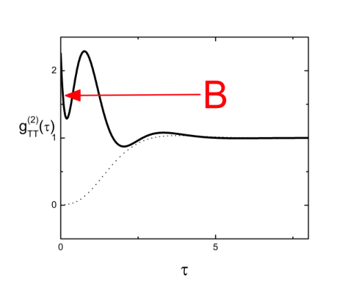
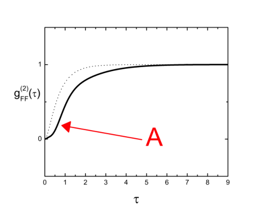
Figure 5: Example of a graph exhibiting Super-Poissonian statistics, denoted “SUP”

The next inequality is derived from the fact that all classical well behaved functions must obey the Schwartz inequality. Because we known that the general form of the Schwartz Inequality is

	$\displaystyle\left(\int dx\int dy\|f(x,y)g(x,y)\|P(x,y)\right)^{2}$	$\displaystyle\leq$	$\displaystyle\left(\int dx\int dy{f(x,y)}^{2}P(x,y)\right)$		(72)
		$\displaystyle\times$	$\displaystyle\left(\int dx\int dy\hskip 8.50012pt{g(x,y)}^{2}P(x,y)\right).$		(72)

We can absorb the probability into a function of $x,y$ and write

	$\displaystyle\left(\int dx\int dy\|\bar{f}(x,y)\bar{g}(x,y)\|\right)^{2}$	$\displaystyle\leq$	$\displaystyle\left(\int dx\int dy{\bar{f}(x,y)}^{2}\right)$		(73)
		$\displaystyle\times$	$\displaystyle\left(\int dx\int dy\hskip 8.50012pt{\bar{g}(x,y)}^{2}\right).$		(73)

By choosing $x=\bar{I}$ , $y=\bar{I}_{0}$ , $f(x,y)=\bar{I}$ , $\quad g(x,y)=1$ , and $P(x,y)=P(\bar{I},t+\tau;\bar{I}_{0},t)$ where $P(\bar{I},t+\tau;\bar{I}_{0},t)$ is the joint probability function that there is field intensity $\bar{I}$ at time $t+\tau$ and intensity $\bar{I}_{0}$ at time $t$ , equation 72 becomes

$\displaystyle\left(\int d\bar{I}\quad\bar{I}P(\bar{I},t+\tau)\right)^{2}$	$\displaystyle\leq$	$\displaystyle\left(\int d\bar{I}\quad{\bar{I}}^{2}P(\bar{I},t+\tau)\right)\times 1$
$\displaystyle{\langle\bar{I}\rangle}^{2}$	$\displaystyle\leq$	$\displaystyle\langle{\bar{I}}^{2}\rangle$
$\displaystyle\frac{\langle{\bar{I}}^{2}\rangle}{{\langle\bar{I}\rangle}^{2}}$	$\displaystyle\geq$	$\displaystyle 1.$	(74)

And now we express the Intensities in terms of the field as

	$\displaystyle\frac{\langle{E^{*}(t)}^{2}{E(t)}^{2}\rangle}{{E^{\ast}(t)E(t)\rangle}^{2}}$	$\displaystyle\geq$	$\displaystyle 1$
	$\displaystyle\frac{\langle{a^{{\dagger}}(t)}^{2}{a(t)}^{2}\rangle}{{\langle{a^{{\dagger}}}(t)a(t)\rangle}^{2}}$	$\displaystyle\geq$	$\displaystyle 1.$		(75)

Because the field is stationary, this can be written as

\frac{\langle{a^{{\dagger}}(t)}^{2}{a(t)}^{2}\rangle}{{\langle{a^{{\dagger}}}a\rangle}^{2}}\geq 1.

(76)

Which is just the expression for $g^{(2)}(\tau)$ at time $t=0$ , so the final inequality is

g^{(2)}(0)\geq 1

(77)

no non-negative probability distributions occur (refer to section for explanation). If $g^{(2)}(0)>1$ our data is super-Poissonian, and if If $g^{(2)}(0)<1$ our data is sub-Poissonian. They shall be referred to as “SUP” and “SUB”. An example of the sub-Poissonian condition is shown in figure 5. Please note specifically the notation used in this section, as some people refer to both of these violations as anti-bunching.

The next set of equalities represent what shall be termed an overshoot “OS” or an undershoot “US”Ṫhese are represented as

	$\displaystyle\|g^{(2)}(\tau)-1\|>\|g^{(2)}(0)-1\|$		(78)
	$\displaystyle\|g^{(2)}(\tau)-1\|<\|g^{(2)}(0)-1\|$		(79)

respectively. An example of each of these is shown (see figures 6, 7).

Figure 6: Overshoot represented by “OS”

II.2 Cross Correlations

There are only two inequalities that must be examined for the cross-correlations. They will be called Cross-Violations, and denoted as “CV1”and “CV2”. A CV1 disobeys the inequality

g^{(2)}_{TF,FT}(0)\leq\sqrt{g^{2}_{TT}(0)g^{2}_{FF}(0)}

(80)

However, because the case being examined is for one atom, $g^{2}_{FF}(0)$ is always zero. This is because of the fact that $\sigma_{-}|e\rangle=|g\rangle$ , and $\sigma_{-}|g\rangle$ is impossible (refer to section ). This simplifies the CV1 to

g^{(2)}_{TF,FT}(0)\leq 0

(81)

in which case there will always be a violation. As for CV2,

g^{2}_{TF}-1\leq\sqrt{|g^{2}_{TT}-1||g^{2}_{FF}-1|}

(82)

which again simplifies to

g^{2}_{TF}-1\leq\sqrt{g^{2}_{TT}-1}

(83)

III Graphs for $g/\gamma=1$ , $\kappa/\gamma=1.6$

Located on each graph will be a small table indicating which non-classical behaviors are present. If a behavior is not listed, it is assumed to be classical. The following is a reminder of each non-classical abbreviation.

B - Bunching

A - Anti-bunching

SUB - Sub-Poissonian probability distribution

SUP - Super-Poissonian probability distribution

OS - Overshoot

US - Undershoot

CV1 - Cross-violation 1

CV2 - Cross-violation 2

Note also that some of the graphs are not smooth lines, but instead have ”wiggles”. What is being seen are the beat frequencies. In the dressed-state picture, each next highest level can be considered an un-coupled three-level system. When these interact, we see the beat frequencies.

IV Inequalities and Non-Classical Behaviors

As described in Section , a violation of the classical behaviors of $h_{\theta}$ are a sign of squeezing (refer to section 7.2.4). Again, the results will be divided into two categories - the transmissions and fluorescence, and the cross correlations.

IV.1 Transmission and Fluorescence

There are only two possible violations to consider [11, 12]. The violations will be denoted as “S1”and “S2”because they both signify squeezing. They are defined respectively as

	$\displaystyle 0\leq h_{\theta}(0)-1\leq 1$		(84)
	$\displaystyle\|h_{\theta}(\tau)-1\|\leq\|h_{\theta}(0)-1\|\leq 1$		(85)

An S1 violation will therefore occur any time the value of $h_{\theta}(0)$ is not between 1 and 2. Note that because the fluorescence condition has an initial value of zero, it will always have an S1 violation. An S2 violation will occur any time the graph dips below zero or rises above two. Furthermore, an S2 violation can occur between a more narrow range of values, dependant upon the initial value, as analogous to overhoot/undershoot violations for $g^{(2)}(\tau)$ . Examples of S1 and S2 violations are shown below

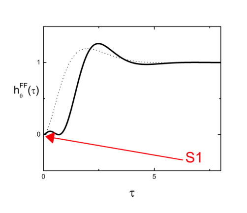
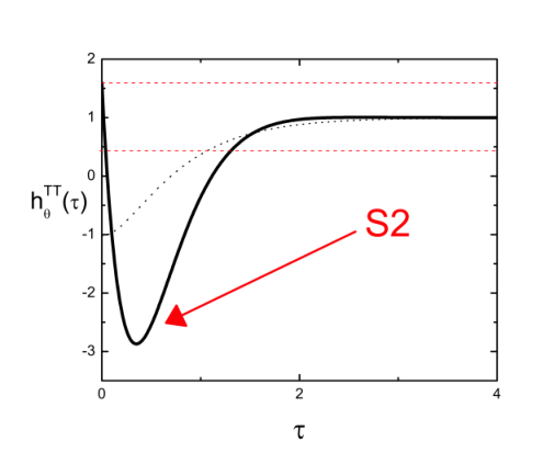
Finally we consider violations of classical inequalities for the cross correlations. These are also readily observed

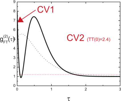
We now present tables that examine which nonclassical effects happen for which parameters

Figure 12: Nonclassical effects in $g^{(2)}(\tau)$ .

V Conclusions

We have investigated intensity-intensity and field-intensity correlations in a cavity QED system with an internal potential with a periodity of $\lambda/1$ where $\lambda$ is the simultaneous wavelength of the atomic transition and cavity mode. When both the atom and cavity are off resonance it was found that the anti-bunching in all the cases disappeared the more off resonance we went. It was found that both the photon statistics and the wave-particle correlation functions are quite sensitive to center-of-mass wave function. This can be eased by choosing atomic and cavity detunings equal and opposite (in units of their respective linewidths). Here nonclassical behavior is not reduced drastically We saw that an increase in the width of the Gaussian in both the SHO and Mahtieu cases washed away non-classicalities with the Mathieu case experiencing more rapid washing out with increase in Gaussian width. In all cases investigated, the correlation functions $g^{(2)}_{FF}$ and $h^{FF}_{\theta}$ appear to be sensitive only to the Mathieu and SHO population distributions for large values of the Gaussian width. The intensity-field fluctuations are not as sensitive to detunings.

References

[1] For a comprehensive review, see Optical Coherence and Quantum Optics, L. Mandel and E. Wolf, Cambridge (2000).
[2] E.T. Jaynes and F.W. Cummings, Proc. IEEE 51, 89 (1963).
[3] Cavity Quantum Electrodynamics, edited by P. Berman, in Advances in Atomic and Molecular Physics, Supplement 2, Academic, San Diego, (1994).
[4] Optical Bistability: Controlling Light With Light (Optics & Photonics Series), Hyatt Gibbs, , Academic Press, 2001.
[5] Introduction to Applied Nonlinear Dynamical Systems and Chaos (Texts in Applied Mathematics) (v. 2) 3rd ed), S. Wiggins, Springer, Berlin, 2000.
[6] H. J. Carmichael, R. J. Brecha, and P. R. Rice, Optics Communications 82, 73 (1991);R. J. Brecha, P. R. Rice, and X. Min, Phys. Rev. A 59, 2392 (1999).
[7] G. Rempe, R. J. Thompson, R. J. Brecha, W. D. Lee, and H. J. Kimble Phys. Rev. Lett. 67, 1727 (1991)
[8] G. T. Foster, S. L. Mielke, and L. A. Orozco Phys. Rev. A 61, 053821 (2000).
[9] A nice introduction is L Guidoni and P Verkerk, J. Opt. B 1, R23 (1999).
[10] J. McKeever, A. Boca, A. D. Boozer, J. R. Buck, and H. J. Kimble, Nature (London) 425, 268 (2003).
[11] adsrar
[12] asdrardsasdr
[13] H. J. Carmichael, An Open Systems Approach To Quantum Optics, (Springer-Verlag, Berlin, 1993), L. Tian and H. J. Carmichael, Phys. Rev. A. 46, R6801 (1992).
[14] D. W. Vernooy and H. J. Kimble Phys. Rev. A 56, 4287-4295 (1997)
[15] H. J. Carmichael, H. M.Castro-Beltran, G. T. Foster, and L. A. Orozco, Phys. Rev. Lett. 85, 1855 (2000).
[16] G. T. Foster, L. A. Orozco, H. J. Carmichael, and H. M. Castro-Beltran, Phys. Rev. Lett. 85, 3149 (2000).