Learning-based Natural Geometric Matching with Homography Prior
Abstract
Geometric matching is a key step in computer vision tasks. Previous learning-based methods for geometric matching concentrate more on improving alignment quality, while we argue the importance of naturalness issue simultaneously. To deal with this, firstly, Pearson correlation is applied to handle large intra-class variations of features in feature matching stage. Then, we parametrize homography transformation with 9 parameters in full connected layer of our network, to better characterize large viewpoint variations compared with affine transformation. Furthermore, a novel loss function with Gaussian weights guarantees the model accuracy and efficiency in training procedure. Finally, we provide two choices for different purposes in geometric matching. When compositing homography with affine transformation, the alignment accuracy improves and all lines are preserved, which results in a more natural transformed image. When compositing homography with non-rigid thin-plate-spline transformation, the alignment accuracy further improves. Experimental results on Proposal Flow dataset show that our method outperforms state-of-the-art methods, both in terms of alignment accuracy and naturalness.
keywords
Geometric matching, convolutional neural network (CNN), Pearson correlation, naturalness, homography*Jing Chen, \linkablechenjing@mail.nankai.edu.cn
1 Introduction
Estimating a geometric matching between images plays a fundamental and important role in computer vision tasks, such as image stitching [1, 2, 3] and image retrieval [4]. Traditional geometric matching methods usually start with a local image descriptor and then estimate geometric model by RANSAC [5]. In general, there are two main procedures for geometric matching: feature characterization, and transformation model selection.
For feature characterization, many hand-crafted image descriptors [6, 7] were proposed in the last decades, which aimed to reliably localize a set of stable local regions under various imaging conditions. However, when intra-class variation of images is large or background is full of cluster, traditional features may fail to generate valid geometric matching.

For transformation model selection, global D transformations such as Euclidean, similarity, affine, and homography have occupied a key position in rigid transformations. Among these transformations, affine has 6 degrees of freedom which maps parallel lines to parallel lines but lacks power of characterizing large viewpoint variations, whereas homography has 8 degrees of freedom which has better alignment, preserve all straight lines, and characterizes viewpoint variations well. To achieve alignment flexibility and accuracy, thin-plate spline (TPS) [9] and as-projective-as-possible (APAP) warp [10], formulate the non-rigid transformation as a matching problem with a smoothness constraint. However, naturalness is also a critical factor which influences the appearance of final transformed image. Non-rigid transformations usually align the source image and target image better than rigid transformations, but they suffer from line-bending and shape-distortion to some extent. As shown in Fig. 2(c), TPS transformation aligns the source image and target image well, at the cost of local distortion (such as curved lines).
Recently, learning-based geometric matching methods [11, 12, 13, 8] have made a great progress on dealing with the limited generalization power of traditional feature descriptors and the low alignment accuracy under large intra-class variations. Unlike [11, 12, 13] which divide the image into local patches and extract descriptors individually, Rocco et al. [8] proposed an end-to-end convolutional neural network architecture, which combines affine and TPS transformations (see Fig. 2(d)) for coarse-to-fine alignment. However, affine transformation is not flexible enough to characterize large viewpoint variations. As shown in Fig. 2(b), the orientation of motorbike after affine transformation looks different from that in target image, whereas homography can characterize this orientation properly (see Fig. 2(f)).
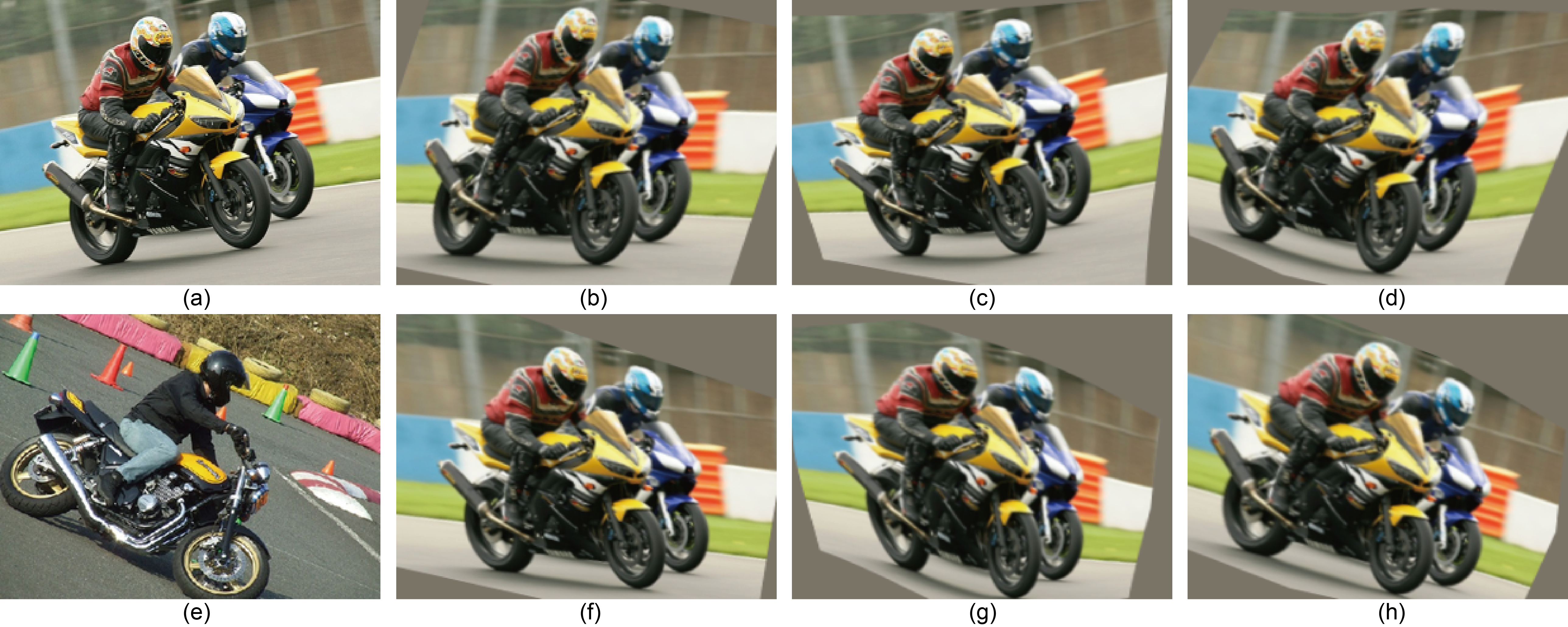
The above alignment and naturalness issues motivate us to construct a geometric matching which aligns images well and produces natural transformed images. Since affine is not powerful for aligning images and characterizing large viewpoint variations, we use homography in our network. The composition of homography and TPS provides better alignment (see Fig. 2(g)) than state-of-the-art methods, while the composition of homography and affine results in a more natural transformed image which preserves all lines (see Fig. 2(h)). In this letter, we propose a novel learning-based architecture, which can be trained end-to-end for natural geometric matching with homography prior. Contributions are summarized as follows:
- 1.
We introduce Pearson correlation for improving the generalization ability of feature matching stage.
- 2.
We add homography transformation to our CNN architecture for learning more flexible rigid transformation.
- 3.
We define a new loss function for training the model, which equips a location dependent Gaussian weight for grid loss [8].
- 4.
Our single homography model achieves the best performance on Proposal Flow dataset, while the compositions of homography and other transformations solve alignment and naturalness issues successfully.
2 Proposed Architecture
In this section, a novel architecture (see Fig. 1) is proposed for natural geometric matching. After extracting the features by CNN, we use Pearson correlation [15] to match features of two input images. Then, we apply the homography transformation with more degrees of freedom to obtain better alignment and more natural transformed images. Finally, a novel loss function guarantees the model accuracy and efficiency in training procedure. Compositing homography with affine or TPS transformation significantly further increases the performance.
2.1 Feature Extraction
Given two input images and with size ( in our architecture), we use ResNet-101 [16] cropped at the layer3 layer (ResNet-101-C4 layer in [16]) to extract deep features in two input images, respectively. Compared to VGG-16 network [17], ResNet-101 has been proven that it can characterize the features better and achieve less error on a majority of datasets.
2.2 Matching with Pearson Correlation
In [8], given L2-normalized dense feature maps , , the correlation map of between features is then characterized by scalar product of individual column vectors. Essentially, let and be the column vectors in and , the above two-step feature normalization and matching procedures can be regard as cosine similarity,
| (1) |
However, cosine similarity is not robust to shifts. If the distribution of or has large intra-class variations, the cosine similarity would change sensitively at the same time, which greatly effects the generalization power of feature matching stage.
Fortunately, in statistics, Pearson correlation [15] can measure the correlation or similarity between two variables and well. Thus, in our feature matching stage, we replace original correlation map of individual descriptor and in [8] with Pearson correlation, i.e.,
| (2) |
where , and are the respective means. The new correlation map alleviates the influence of large intra-class variations, and then makes our matching stage more general and robust under different conditions.
2.3 Transformation Model Selection
Estimating a geometric transformation is a challenging task in deep learning in recent years, since selecting a proper transformation is not intuitive and always needs more considerations about variations of different scenes. As mentioned above, considering the disadvantages of affine and TPS, we use homography transformation, which is known as the most flexible rigid transformation, in our geometric matching architecture for better alignment and more natural transformed images.
Generally, we can parametrize homography to be parameters, which contains a matrix with a fixed scale constraint [13]. As pointed in [18], it is not necessary and advisable to use minimal parametrization since the surface of the cost function usually becomes more complicated when minimal parametrizations are used. Thus, we parametrize homography transformation with parameters, i.e, a matrix with the following form
| (3) |
and allow the last parameter to be an arbitrary real number.
Compared to affine and TPS transformations, homography has a better alignment ability and viewpoint characterization than affine, and can preserve all lines while TPS always fails. After compositing homography with affine and TPS transformations in [8], we have two choices: affine + homography, and homography + TPS. Compared with affine + TPS in [8], the first choice results in a more natural transformed image (see Fig. 2), and the second choice achieves better alignment accuracy (see Tab. 1).
2.4 Loss Function
Let and denote the ground truth and the estimated transformations with parameters and , respectively. Rocco et al. [8] proposed a grid loss which measures the discrepancy between the two transformed imaginary grids by
| (4) |
where is the set of grid point from to with the step , and is the number of grid points, i.e., .
We mimic the classical approach APAP [10] which uses Gaussian weights to give higher importance to data that are closer to features for better alignment. Since objects always locate in the center of the image, we give higher weights to respects the local structure around the center of grid points (see Fig. 3), and the weight in grid is calculated as
| (5) |
Thus, our loss is defined as
| (6) |
Since is trainable with respect to the parameters of homography, our loss is differentiable with respect to in a straightforward manner.
3 Experimental Evaluation
In this section, we compare proposed architecture against CNN geometric matching methods [8] and several state-of-the-art geometric matching methods [19, 20, 21, 22, 14] on Proposal Flow dataset [14]. Moreover, ablation studies further show the advantages of proposed method.
In our experiment, we set hyper-parameters following existing architecture as [8], set to be , and to be in Eq. (6) since the grids range from . Codes are implemented in PyTorch [23], and based on the code 11 1 http://github.com/ignacio-rocco/cnngeometric_pytorch of [8].

| Methods | PCK (%) |
|---|---|
| DeepFlow [22] | 20 |
| GMK [19] | 27 |
| SIFT Flow [20] | 38 |
| DSP [21] | 29 |
| Proposal Flow NAM [14] | 53 |
| Proposal Flow PHM [14] | 55 |
| Proposal Flow LOM [14] | 56 |
| VGG + CNNGeo. (affine) [8] | 49 |
| ResNet-101 + CNNGeo. (affine) [8] | 56 |
| ResNet-101 + CNNGeo. (TPS) [8] | 58 |
| ResNet-101 + Ours (homo) | 61 |
| VGG + CNNGeo. (affine + TPS) [8] | 56 |
| ResNet-101 + CNNGeo. (affine + TPS) [8] | 68 |
| ResNet-101 + Ours (homo + affine) | 65 |
| ResNet-101 + Ours (homo + TPS) | 69 |
| Methods | Pascal-synth-homo |
|---|---|
| Matching with cosine similarity [8] | 58 |
| Homography with parameters | 55 |
| Training with MSE loss | 55 |
| Training with grid loss | 59 |
| Ours with our loss + Pearson correlation + parameters | 61 |
3.1 Datasets and Evaluation Criterion
We train the proposed network for homography on Pascal VOC 2011 by strongly supervised learning, with the generated dataset Pacal-synth-homo. For each image in the dataset, we randomly perturb the four corners of the image within image, then computed a relative homography matrix by the coordinates of four corners. Thus, each data contains a source image, a homography matrix with numbers, and a transformed image by homography. To evaluate the proposed architecture, we follow the standard criterion, the average probability of correct keypoint (PCK) [24], which computes the proportion of keypoints that are correctly matched.
3.2 Comparisons with state-of-the-arts
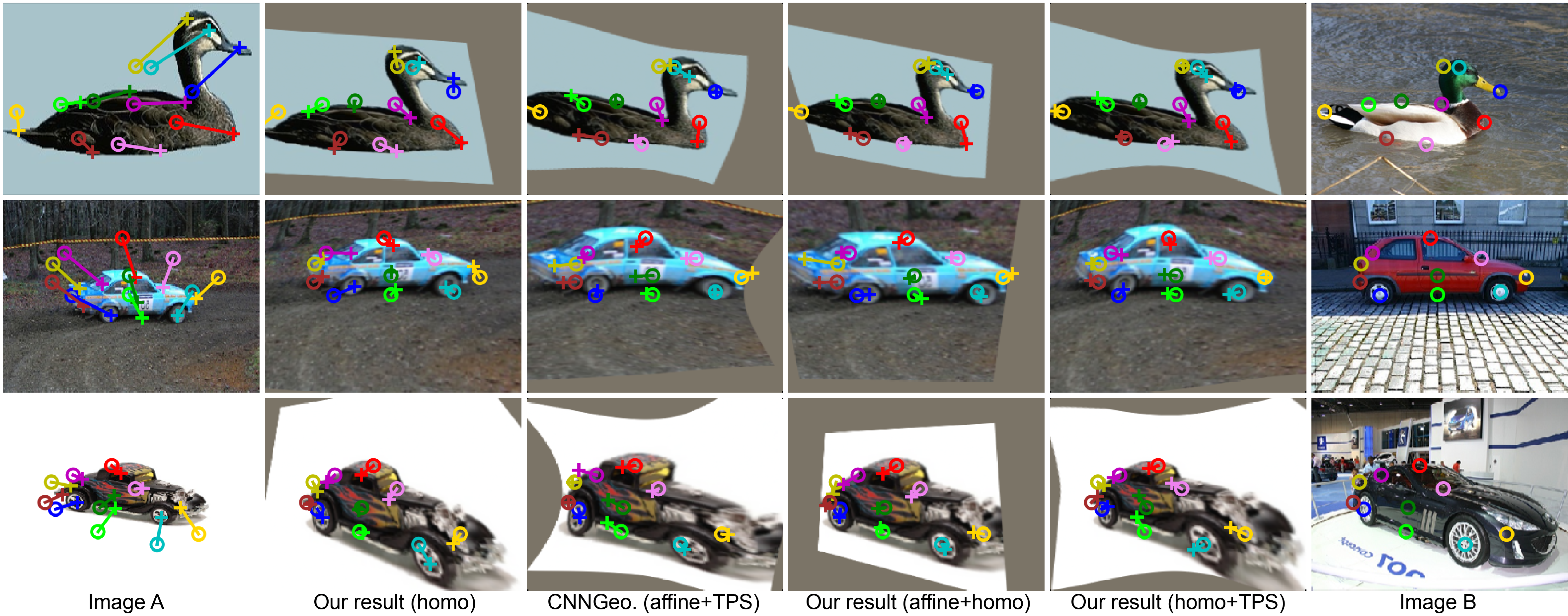
We run a number of comparisons to analyze the proposed architecture. As shown in Tab. 1, our architecture with single homography reaches the first place in all single model. When compositing with TPS, our architecture achieves better performance than the competing methods in [8] which composites affine and TPS. Note that the ResNet-101-based model in [8] uses larger datasets, and is composed of many other strategies, while our model does not use them but still performs better. Although compositing our homography with affine does not get the best performance, it is still meaningful when considering the naturalness issue, especially when the scenes is full of line structures.
3.3 Ablation Studies
Extensive ablation studies are conducted to validate how each of these changes contribute to our overall architecture, as shown in Tab. 2. When matching with cosine similarity as [8], the performance drops percent. After parametrizing homography with degrees of freedom instead of , the PCK increases significantly. Moreover, our loss function effectively improves the performance compared to grid loss and MSE loss.
4 Conclusion
We propose a novel architecture for natural geometric matching with homography prior, which uses Pearson correlation to match features of two input images, parametrizes the homography transformation with more degrees of freedom, and applies a novel loss function to guarantee the model accuracy and efficiency in training procedure. Compositing our homography prior with affine or TPS transformation significantly increases the performance both on alignment accuracy and naturalness. Future works include making the separate training of homography and other transformations in a unified framework.
References
- [1] M. Brown and D. G. Lowe, “Automatic panoramic image stitching using invariant features,” Int. J. Comput. Vis. 74(1), 59–73 (2007).
- [2] J. An, H. I. Koo, and N. I. Cho, “Unified framework for automatic image stitching and rectification,” J. Electron. Imaging 24(3), 033007 (2015).
- [3] N. Li, Y. Xu, and C. Wang, “Quasi-homography warps in image stitching,” IEEE Trans. Multimedia 20(6), 1365–1375 (2018).
- [4] L. Feng, L. Yu, and H. Zhu, “Spectral embedding-based multiview features fusion for content-based image retrieval,” J. Electron. Imaging 26(5), 1 (2017).
- [5] M. A. Fischler and R. C. Bolles, “Random sample consensus: A paradigm for model fitting with applications to image analysis and automated cartography,” Commun. ACM 24(6), 381–395 (1981).
- [6] D. G. Lowe, “Distinctive image features from scale-invariant keypoints,” Int. J. Comput. Vis. 60(2), 91–110 (2004).
- [7] H. Bay, T. Tuytelaars, and L. Van Gool, “SURF: Speeded up robust features,” in Proc. ECCV, 404–417, Springer (2006).
- [8] I. Rocco, R. Arandjelovic, and J. Sivic, “Convolutional neural network architecture for geometric matching,” in Proc. IEEE CVPR, 39–48 (2017).
- [9] F. L. Bookstein, “Principal warps: Thin-plate splines and the decomposition of deformations,” IEEE Trans. Pattern Anal. Mach. Intell. 11(6), 567–585 (1989).
- [10] J. Zaragoza, T.-J. Chin, Q.-H. Tran, et al., “As-projective-as-possible image stitching with moving DLT,” IEEE Trans. Pattern Anal. Mach. Intell. 36(7), 1285–1298 (2014).
- [11] X. Han, T. Leung, Y. Jia, et al., “Matchnet: Unifying feature and metric learning for patch-based matching,” in Proc. IEEE CVPR, 3279–3286 (2015).
- [12] E. Simo-Serra, E. Trulls, L. Ferraz, et al., “Discriminative learning of deep convolutional feature point descriptors,” in Proc. IEEE ICCV, 118–126 (2015).
- [13] D. DeTone, T. Malisiewicz, and A. Rabinovich, “Deep image homography estimation,” arXiv preprint arXiv:1606.03798 (2016).
- [14] B. Ham, M. Cho, C. Schmid, et al., “Proposal Flow,” in Proc. IEEE CVPR, 3475–3484 (2016).
- [15] K. Pearson, “Note on regression and inheritance in the case of two parents,” Proceedings of the Royal Society of London 58, 240–242 (2006).
- [16] K. He, X. Zhang, S. Ren, et al., “Deep residual learning for image recognition,” in Proc. IEEE CVPR, 770–778 (2016).
- [17] K. Simonyan and A. Zisserman, “Very deep convolutional networks for large-scale image recognition,” in Proc. ICLR, 1,2 (2015).
- [18] R. Hartley and A. Zisserman, Multiple view geometry in computer vision, Cambridge univ. press (2003).
- [19] O. Duchenne, A. Joulin, and J. Ponce, “A graph-matching kernel for object categorization,” in Proc. IEEE ICCV, 1792–1799, IEEE (2011).
- [20] C. Liu, J. Yuen, and A. Torralba, “Sift flow: Dense correspondence across scenes and its applications.,” IEEE Trans. Pattern Anal. Mach. Intell. 33(5), 978 (2011).
- [21] J. Kim, C. Liu, F. Sha, et al., “Deformable spatial pyramid matching for fast dense correspondences,” in Proc. IEEE CVPR, 2307–2314 (2013).
- [22] J. Revaud, P. Weinzaepfel, Z. Harchaoui, et al., “DeepMatching: Hierarchical deformable dense matching,” Int. J. Comput. Vis. 120(3), 300–323 (2016).
- [23] A. Paszke, S. Gross, S. Chintala, et al., “Pytorch.” http://pytorch.org/ (2017).
- [24] Y. Yang and D. Ramanan, “Articulated human detection with flexible mixtures of parts,” IEEE Trans. Pattern Anal. Mach. Intell. 35(12), 2878–2890 (2013).