跳到论文正文
W Papers独立论文阅读器 arXiv:1807.04612 论文正文 计算阅读时间 · 0%
引用这篇论文根据当前论文元数据生成,正式投稿前建议核对。


License: arXiv.org perpetual non-exclusive license
arXiv:1807.04612v2 [q-fin.MF] 10 May 2019

Pricing without martingale measure

Julien Baptiste    Laurence Carassus    Emmanuel Lépinette
Abstract

For several decades, the no-arbitrage (NA) condition and the martingale measures have played a major role in the financial asset’s pricing theory. We propose a new approach for estimating the super-replication cost based on convex duality instead of martingale measures duality : Our prices will be expressed using Fenchel conjugate and bi-conjugate. The super-hedging problem leads endogenously to a weak condition of NA called Absence of Immediate Profit (AIP). We propose several characterizations of AIP and study the relation with the classical notions of no-arbitrage. We also give some promising numerical illustrations.

keywords
Financial market models , Super-hedging prices , No-arbitrage condition , Conditional support , Essential supremum. 2000 MSC: 60G44 , G11-G13

?? Paris Dauphine university, PSL research university, Ceremade, CNRS, UMR, Place du Maréchal De Lattre De Tassigny, 75775 Paris cedex 16, France.
Email: baptiste@ceremade.dauphine.fr, emmanuel.lepinette@ceremade.dauphine.fr

??Léonard de Vinci Pôle Universitaire, Research Center, 92 916 Paris La Défense, France
and LMR, université de Reims-Champagne Ardenne, France
Email: laurence.carassus@devinci.fr

??Gosaef, Faculté des Sciences de Tunis, 2092 Manar II-Tunis, Tunisia.

1 Introduction

The problem of giving a fair price to a financial asset GG is central in the economic and financial theory. A selling price should be an amount which is enough to initiate a hedging strategy for GG, i.e. a strategy whose value at maturity is always above GG. It seems also natural to ask for the infimum of such amount. This is the so called super-replication price and it has been introduced in the binomial setup for transaction costs by [7]. Characterizing and computing the super-replication price has become one of the central issue in mathematical finance theory. Until now it was intimately related to the No-Arbitrage (NA) condition. This condition asserts that starting from a zero wealth it is not possible to reach a positive one (non negative almost surely and strictly positive with strictly positive probability measure). Characterizing the NA condition or, more generally, the No Free Lunch condition leads to the Fundamental Theorem of Asset Pricing (FTAP in short). This theorem proves the equivalence between those absence of arbitrage conditions and the existence of equivalent risk-neutral probability measures (also called martingale measures or pricing measures) which are equivalent probability measures under which the (discounted) asset price process is a martingale. This was initially formalised in [13], [14] and [20] while in [10] the FTAP is formulated in a general discrete-time setting under the NA condition. The literature on the subject is huge and we refer to [11] and [17] for a general overview. Under the NA condition, the super-replication price of GG is equal to the supremum of the (discounted) expectation of GG computed under the risk-neutral probability measures. This is the so called dual formulation of the super-replication price or superhedging theorem. We refer to [29] and [12] and the references therein.

In this paper, a super-hedging or super-replicating price is the initial value of some super-hedging strategy. We do not postulate any assumption on the financial market and analyze from scratch the set of super-hedging prices and its infimum value, which will be called the infimum super-hedging cost. Under mild assumptions, we show that the one-step set of super-hedging prices can be expressed using Fenchel-Legendre conjugate and the infimum super-replication cost is obtained by the Fenchel-Legendre biconjugate. So, we use here the convex duality instead of the usual financial duality based on martingale measures under the NA condition. To do so, we use the notion of conditional essential supremum. Using measurable selection techniques, we show that the conditional essential supremum of a function of YY is equal to the usual supremum of the function evaluated on a random set, the conditional support of YY (see Proposition 2.9). The pricing formula that we obtain (see (2.14)) shows that, if the initial stock price yy does not belong to the convex hull of the conditional support of the stock value at the end of the period Y,Y, then the super-hedging cost is equal to −∞-\infty. To exclude this possibility we postulate the condition of Absence of Immediate Profit (AIP). The AIP is an endogenous condition for pricing and is indeed very weak : If the initial information is trivial, a one period immediate profit is a strategy which starts from 0 and leads to a deterministic strictly positive gain at time 1. We propose several characterization of the AIP condition. In particular we show that AIP is equivalent to the non-negativity of the super-hedging prices of any fixed call option. We also discuss in details the link between AIP and the others no-arbitrage conditions as the no-arbitrage of first and second type and the no-riskless arbitrage of [15] and the No Unbounded Profit with Bounded Risk of [19]. None of the conditions is equivalent to AIP, the closest being the no-riskless arbitrage. Under AIP condition, we show that the one-step infimum super-hedging cost is the concave envelop of the payoff relatively to the convex envelop of the conditional support. Fenchel-Legendre duality have already been used to obtain a dual representation of the super-replication price thanks to deflators (see [24, Exemple 4.2] and [25, Theorem 10 and Corollary 15]). In [25, Theorem 10] the result is shown under the assumption that the set of claims that can be super-replicate from 00 is closed, which holds true under NA. Our approach is different as we do not postulate any assumption on the market and, actually, we do not seek for a dual representation of the (minimal) super-hedging price.

We then consider the multiple-period framework. We show that the global AIP condition and the local ones are equivalent. We study the link between AIP, NA and the absence of weak immediate profit (AWIP) conditions. We show that the AIP condition is the weakest-one and we also provide conditions for the equivalence between the AIP and the AWIP conditions, as well as characterization through absolutely continuous martingale measure.

We then focus on a particular, but still general setup, where we propose a recursive scheme for the computation of the super-hedging prices of a convex option. We obtain the same computation scheme as in [8] and [9] but here it is obtained by only assuming AIP instead of the stronger NA condition. We also give some numerical illustrations. We calibrate historical data of the french index CAC 4040 to our model and implement our super-hedging strategy for a call option. Our procedure is somehow model free as it is only based on statistical estimations.

The paper is organized as follows. In Section 2, we study the one-period framework while in Section 3 we study the multi-period one. Section 4 proposes an explicit pricing for a convex payoff and numerical experiments.

In the remaining of this introduction we present our framework and notations. Let (Ω,(ℱt)t∈{0,…,T}​ℱT,P)(\Omega,({\cal F}_{t})_{t\in\{0,\ldots,T\}}{\cal F}_{T},P) be a complete filtered probability space, where TT is the time horizon. For any σ\sigma-algebra ℋ{\cal H} and any k≥1k\geq 1, we denote by L0​(ℝk,ℋ)L^{0}({\mathbb{R}}^{k},{\cal H}) the set of ℋ{\cal H}-measurable and ℝk{\mathbb{R}}^{k}-valued random variables. We consider a non-negative process S:={St,t∈{0,…,T},}S:=\left\{S_{t},\ t\in\{0,\ldots,T\},\right\} such that St∈L0​(ℝd,ℱt)S_{t}\in L^{0}({\mathbb{R}}^{d},{\cal F}_{t}) for all t∈{0,…,T}t\in\{0,\ldots,T\}. The vector StS_{t} represents the price at time tt of the dd risky assets in the financial market in consideration. Trading strategies are given by a process θ:={θt,t∈{0,…,T−1},}\theta:=\{\theta_{t},t\in\{0,\ldots,T-1\},\} such that θt∈L0​(ℝd,ℱt)\theta_{t}\in L^{0}({\mathbb{R}}^{d},{\cal F}_{t}) for all t∈{0,…,T−1},t\in\{0,\ldots,T-1\},. The vector θt\theta_{t} represents the investor’s holding in the dd risky assets between time tt and time t+1t+1. We assume that trading is self-financing and that the riskless asset’s price is a constant equal to 11. The value at time tt of a portfolio θ\theta starting from initial capital x∈ℝx\in\mathbb{R} is then given by

Vtx,θ=x+∑u=1tθu−1​Δ​Su,V^{x,\theta}_{t}=x+\sum_{u=1}^{t}\theta_{u-1}\Delta S_{u},

where Δ​Su=Su−Su−1\Delta S_{u}=S_{u}-S_{u-1} for u≥1u\geq 1 and x​yxy is the scalar product of xx and yy.

2 The one-period framework

Let ℋ{\cal H} and ℱ{\cal F} be two complete sub-σ\sigma-algebras of ℱT{\cal F}_{T} such that ℋ⊆ℱ{\cal H}\subseteq{\cal F} and which represent respectively the initial and the final information. Let y∈L0​(ℝd,ℋ)y\in L^{0}({\mathbb{R}}^{d},{\cal H}) and Y∈L0​(ℝd,ℱ)Y\in L^{0}({\mathbb{R}}^{d},{\cal F}) be two non-negative11 1 For ease of notation, we assume that y⁡(ω)≥0y(\omega)\geq 0 and Y⁡(ω)≥0Y(\omega)\geq 0 for all ω∈Ω\omega\in\Omega. random variables. They represents the initial and the final prices of the dd risky assets. Finally, we introduce g:Ω×ℝ→ℝg:\Omega\times{\mathbb{R}}\to{\mathbb{R}} and the associated derivative g⁡(Y)g(Y), where g⁡(Y):ω→g⁡(Y)​(ω)=g⁡(ω,Y⁡(ω)).g(Y):\omega\to g(Y)(\omega)=g(\omega,Y(\omega)).
The objective of the section is to obtain under suitable assumptions on gg a characterization of 𝒫⁡(g){\cal P}(g), the one-step set of super-hedging (or super-replicating) prices of g⁡(Y)g(Y) and of its infimum value. The setting will be applied in Section 3 with the choices ℋ=ℱt{\cal H}={\cal F}_{t}, ℱ=ℱt+1{\cal F}={\cal F}_{t+1}, Y=St+1Y=S_{t+1} and y=Sty=S_{t}.

Definition 2.1.

The set 𝒫⁡(g){\cal P}(g) of super-hedging prices of the contingent claim g⁡(Y)g(Y) consists in the initial values of super-hedging strategies θ\theta:

𝒫(g)={x∈L0(ℝ,ℋ),∃θ∈L0(ℝd,ℋ),x+θ(Y−y)≥g(Y)a.s.}.{\cal P}(g)=\{x\in L^{0}({\mathbb{R}},{\cal H}),\exists\,\theta\in L^{0}({\mathbb{R}}^{d},{\cal H}),\;x+\theta(Y-y)\geq g(Y)\,{\rm a.s.}\}.

The infimum super-hedging cost of g⁡(Y)g(Y) is defined by p⁡(g):=ess​infℋ​𝒫​(g)p(g):=\mathrm{ess\,inf}_{{\cal H}}{\cal P}(g).

The notions of conditional essential infimum ess​infℋ\mathrm{ess\,inf}_{{\cal H}} and conditional essential supremum ess​supℋ\mathrm{ess\,sup}_{{\cal H}} are at the heart of this study and will be defined in Proposition 2.5 below. We will also use the conditional support of YY suppℋ​Y{\rm supp}_{{\cal H}}Y which is introduced in Definition 2.2 below. In Section 2.2, we derive the characterization of 𝒫⁡(g){\cal P}(g) and p⁡(g)p(g) from the following steps :

  1. 1.

    Observe that the set of super-hedging prices can be rewritten using a conditional essential supremum (see (2.8)).

  2. 2.

    Show that under mild conditions the conditional essential supremum of a function of YY is equal to the usual supremum of the function evaluated on the random set suppℋ​Y{\rm supp}_{{\cal H}}Y (see Proposition 2.9).

  3. 3.

    Recognize that a super-hedging price can be written using a Fenchel-Legendre conjugate (see (2.9)).

  4. 4.

    Take the essential infimum of the set of super-hedging prices and go through the three first steps to recognize the Fenchel-Legendre biconjugate (see (2.11)).

  5. 5.

    Use the classical convex biconjugate theorem (see (2.12) and Proposition 2.15) to evaluate the infimum super-hedging cost.

With this pricing formula in hand (see (2.14)), the condition of Absence of Immediate Profit (AIP) appears endogenously. In Section 2.3, we develop the concept of AIP and propose several characterization of the AIP condition and compare it with the classical No Arbitrage NA condition.

2.1 Conditional support and conditional essential infimum

This section is the toolbox of the paper. We recall some results and notations that will be used without further references in the rest of the paper. Let h:Ω×ℝd→ℝh:\Omega\times{\mathbb{R}}^{d}\to{\mathbb{R}}. The effective domain of h⁡(ω,⋅)h(\omega,\cdot) is defined by

dom​h​(ω,⋅):={x∈ℝd,h⁡(ω,x)<∞}{\rm dom\,}h(\omega,\cdot):=\{x\in{\mathbb{R}}^{d},\,h(\omega,x)<\infty\}

and h⁡(ω,⋅)h(\omega,\cdot) is proper if dom h⁡(ω,⋅)≠∅h(\omega,\cdot)\neq\emptyset and h⁡(ω,x)>−∞h(\omega,x)>-\infty for all x∈ℝdx\in{\mathbb{R}}^{d}. Next, if hh is ℋ{\cal H}-normal integrand (see Definition 14.27 in [28]) then hh is ℋ⊗ℬ⁡(ℝd){\cal H}\otimes{\cal B}({\mathbb{R}}^{d})-measurable and is lower semi-continuous (l.s.c. in the sequel, see [28, Definition 1.5]) in xx and the converse holds true if ℋ{\cal H} is complete for some measure, see [28, Corollary 14.34]. Note that, if Z∈L0​(ℝd,ℋ)Z\in L^{0}({\mathbb{R}}^{d},{\cal H}) and hh is ℋ⊗ℬ⁡(ℝd){\cal H}\otimes{\cal B}({\mathbb{R}}^{d})-measurable, then h⁡(Z)∈L0​(ℝd,ℋ)h(Z)\in L^{0}({\mathbb{R}}^{d},{\cal H}).
A random set 𝒦:Ω↠ℝd{\cal K}:\Omega\twoheadrightarrow\mathbb{R}^{d} is said ℋ{\cal H}-measurable if for all open set OO of ℝd{\mathbb{R}}^{d}, the subset {ω∈Ω,O∩𝒦(ω)≠∅}∈ℋ\{\omega\in\Omega,\,O\cap{\cal K}(\omega)\neq\emptyset\}\in{\cal H}. If 𝒦{\cal K} is a ℋ{\cal H}-measurable and closed-valued random set of ℝd{\mathbb{R}}^{d}, then 𝒦{\cal K} admits a Castaing representation (ηn)n∈ℕ(\eta_{n})_{n\in\mathbb{N}} (see Theorem 14.5 in [28]). This means that 𝒦⁡(ω)=cl⁡{ηn​(ω),n∈𝐍}{\cal K}(\omega)={\rm cl}\{\eta_{n}(\omega),\,n\in\mathbf{N}\} for all ω∈dom𝒦={ω∈Ω,𝒦(ω)∩ℝd≠∅}\omega\in{\rm dom\,}{\cal K}=\{\omega\in\Omega,\,{\cal K}(\omega)\cap{\mathbb{R}}^{d}\neq\emptyset\}, where the closure is taken in ℝd{\mathbb{R}}^{d}.

First, we introduce the conditional support of X∈L0​(ℝd,ℱ)X\in L^{0}({\mathbb{R}}^{d},{\cal F}) with respect to ℋ{\cal H}.

Definition 2.2.

Let μ\mu be a ℋ{\cal H}-stochastic kernel (i.e. for all ω∈Ω\omega\in\Omega, μ⁡(⋅,ω)\mu(\cdot,\omega) is a probability on ℬ⁡(ℝd){\cal B}({\mathbb{R}}^{d}) and μ⁡(A,⋅)\mu(A,\cdot) is ℋ{\cal H}-measurable for all A∈ℬ⁡(ℝd)A\in{\cal B}({\mathbb{R}}^{d})). We define the random set Dμ:Ω↠ℝd{D}_{\mu}:\Omega\twoheadrightarrow\mathbb{R}^{d} by :

Dμ​(ω):=⋂{A⊂ℝd,closed,μ⁡(A,ω)=1}.\displaystyle{D}_{\mu}(\omega):=\bigcap\left\{A\subset\mathbb{R}^{d},\;\mbox{closed},\;\mu(A,\omega)=1\right\}. (2.1)

For ω∈Ω\omega\in{\Omega}, Dμ​(ω)⊂ℝd{D}_{\mu}(\omega)\subset\mathbb{R}^{d} is called the support of μ⁡(⋅,ω)\mu(\cdot,\omega).
Let X∈L0​(ℝd,ℱ)X\in L^{0}({\mathbb{R}}^{d},{\cal F}), we denote by suppℋ​X\mathrm{supp\,}_{{\cal H}}X the set defined in (2.1) when μ⁡(A,ω)=P⁡(X∈A|ℋ)​(ω)\mu(A,\omega)=P(X\in A|\mathcal{H})(\omega) is a regular version of the conditional law of XX knowing ℋ{\cal H}. The random set suppℋ​X\mathrm{supp\,}_{{\cal H}}X is called the conditional support of XX with respect to ℋ{\cal H}.

Remark 2.3.

When ℋ{\cal H} is the trivial sigma-algebra, suppℋ​X\mathrm{supp\,}_{{\cal H}}X is just the usual support of XX (see p441 of [1]). Theorems 12.7 and 12.14 of [1] show that P(X∈.|ℋ)P(X\in.|\mathcal{H}) admits a unique support suppℋ​X⊂ℝd\mathrm{supp\,}_{{\cal H}}X\subset\mathbb{R}^{d} such that we have P⁡(X∈suppℋ​X|ℋ)=1P(X\in\mathrm{supp\,}_{{\cal H}}X|\mathcal{H})=1 a.s. i.e. suppℋ​X{\rm supp}_{{\cal H}}X is a.s. non-empty.
For simplicity we will assumed that Y⁡(ω)∈suppℋ​Y​(ω)Y(\omega)\in\mathrm{supp\,}_{{\cal H}}Y(\omega) for all ω∈Ω\omega\in\Omega. Moreover, as 0≤Y<∞0\leq Y<\infty, Dom​suppℋ​Y=Ω{\rm Dom\;supp\;}_{{\cal H}}Y=\Omega.

Lemma 2.4.

DμD_{\mu} is non-empty, closed-valued, ℋ\mathcal{H}-measurable and graph-measurable random set (i.e. G​r​a​p​h​(Dμ)∈ℋ⊗ℬ⁡(ℝd)Graph(D_{\mu})\in\mathcal{H}\otimes\mathcal{B}(\mathbb{R}^{d})).

Proof. It is clear from (2.1) that, for all ω∈Ω\omega\in\Omega, Dμ​(ω)D_{\mu}(\omega) is a non-empty and closed subset of ℝd\mathbb{R}^{d}. We show that DμD_{\mu} is ℋ\mathcal{H}-measurable. Let OO be a fixed open set in ℝd\mathbb{R}^{d} and μO:ω∈Ω↦μO​(ω):=μ⁡(O,ω).\mu_{O}:\omega\in\Omega\mapsto\mu_{O}(\omega):=\mu(O,\omega). As μ\mu is a stochastic kernel, μO\mu_{O} is ℋ\mathcal{H}-measurable. By definition of Dμ​(ω)D_{\mu}(\omega) we get that {ω∈Ω,Dμ(ω)∩O≠∅}={ω∈Ω,μO(ω)>0}∈ℋ,\{\omega\in\Omega,\;{D}_{\mu}(\omega)\cap O\neq\emptyset\}=\{\omega\in\Omega,\;\mu_{O}(\omega)>0\}\in\mathcal{H}, and DμD_{\mu} is ℋ\mathcal{H}-measurable. Now using Theorem 14.8 of [28], G​r​a​p​h​(Dμ)∈ℋ⊗ℬ⁡(ℝd)Graph(D_{\mu})\in\mathcal{H}\otimes\mathcal{B}(\mathbb{R}^{d}) (recall that DμD_{\mu} is closed-valued) and DμD_{\mu} is ℋ\mathcal{H}-graph-measurable. □\Box

It is possible to incorporate measurability in the definition of the essential supremum (see [17, Section 5.3.1] for the definition and the proof of existence of the classical essential supremum). This has been done by [3] for a single real-valued random variable and by [18] for a family of vector-valued random variables and with respect to a random partial order (see [18, Definition 3.1 and Lemma 3.9]). Proposition 2.5 is given and proved for sake of completeness and for pedagogical purpose. The authors thanks T. Jeulin who suggested this (elegant) proof.

Proposition 2.5.

Let ℋ⊆ℱ{\cal H}\subseteq{\cal F} be two σ\sigma-algebras on a probability space. Let Γ=(γi)i∈I\Gamma=(\gamma_{i})_{i\in I} be a family of real-valued ℱ{\cal F}-measurable random variables. There exists a unique ℋ{\cal H}-measurable random variable γℋ∈L0​(ℝ∪{∞},ℋ)\gamma_{{\cal H}}\in L^{0}({\mathbb{R}}\cup\{\infty\},{\cal H}) denoted ess​supℋ​Γ\mathrm{ess\,sup}_{{\cal H}}\Gamma which satisfies the following properties:

  1. 1.

    For every i∈Ii\in I, γℋ≥γi\gamma_{{\cal H}}\geq\gamma_{i} a.s.

  2. 2.

    If ζ∈L0​(ℝ∪{∞},ℋ)\zeta\in L^{0}({\mathbb{R}}\cup\{\infty\},{\cal H}) satisfies ζ≥γi\zeta\geq\gamma_{i} a.s. ∀i∈I\forall i\in I, then ζ≥γℋ\zeta\geq\gamma_{{\cal H}} a.s.

The conditional essential infimum ess​infℋ​Γ\mathrm{ess\,inf}_{{\cal H}}\Gamma is defined symmetrically.

Proof. Considering the homeomorphism arctan\arctan we can restrict our-self to γi\gamma_{i} taking values in [0,1][0,1]. We denote by Pγi|ℋP_{\gamma_{i}|{\cal H}} a regular version of the conditional law of γi\gamma_{i} knowing ℋ{\cal H}. Let ζ∈L0​(ℝ∪{∞},ℋ)\zeta\in L^{0}({\mathbb{R}}\cup\{\infty\},{\cal H}) such that ζ≥γi\zeta\geq\gamma_{i} a.s. ∀i∈I\forall i\in I. This is equivalent to Pγi|ℋ(]−∞,x])|x=ζ=1 a.s. P_{\gamma_{i}|{\cal H}}(]-\infty,x])|_{x=\zeta}=1\mbox{ a.s. } and suppℋγi⊂]−∞,ζ]\mathrm{supp\,}_{{\cal H}}\gamma_{i}\subset]-\infty,\zeta] a.s. follows from Definition 2.2. Let

Λγi|ℋ=sup{x∈[0,1],x∈suppℋ​γi}.\displaystyle\Lambda_{\gamma_{i}|{\cal H}}=\sup\{x\in[0,1],\,x\in\mathrm{supp\,}_{{\cal H}}\gamma_{i}\}. (2.2)

Then Λγi|ℋ≤ζ\Lambda_{\gamma_{i}|{\cal H}}\leq\zeta a.s. and it is easy to see that Λγi|ℋ\Lambda_{\gamma_{i}|{\cal H}} is ℋ{\cal H}-measurable. So taking the classical essential supremum, we get that ess​supi​Λγi|ℋ≤ζ\mathrm{ess\,sup}_{i}\Lambda_{\gamma_{i}|{\cal H}}\leq\zeta a.s. and that ess​supi​Λγi|ℋ\mathrm{ess\,sup}_{i}\Lambda_{\gamma_{i}|{\cal H}} is ℋ{\cal H}-measurable. We conclude that γℋ=ess​supi​Λγi|ℋ\gamma_{{\cal H}}=\mathrm{ess\,sup}_{i}\Lambda_{\gamma_{i}|{\cal H}} a.s. since for every i∈Ii\in I, P⁡(γi∈suppℋ​γi|ℋ)=1P(\gamma_{i}\in\mathrm{supp\,}_{{\cal H}}\gamma_{i}|{\cal H})=1 (see Remark 2.3).□\Box

Remark 2.6.

Let QQ be an absolutely continuous probability measure with respect to PP. Let Z=d​Q/d​PZ=dQ/dP and 𝔼Q\mathbb{E}_{Q} be the expectation under QQ. As for every i∈Ii\in I, ess​supℋ​Γ≥γi\mathrm{ess\,sup}_{{\cal H}}\Gamma\geq\gamma_{i} a.s. and ess​supℋ​Γ\mathrm{ess\,sup}_{{\cal H}}\Gamma is ℋ{\cal H}-measurable,

ess​supℋ​Γ≥𝔼⁡(Z​γi|ℋ)𝔼⁡(Z|ℋ)=𝔼Q​(γi|ℋ).\displaystyle\mathrm{ess\,sup}_{{\cal H}}\Gamma\geq\frac{\mathbb{E}(Z\gamma_{i}|{\cal H})}{\mathbb{E}(Z|{\cal H})}=\mathbb{E}_{Q}(\gamma_{i}|{\cal H}). (2.3)

Inspired by Theorem 2.8 in [3], we may easily show the following tower law property.

Lemma 2.7.

Let ℋ1⊆ℋ2⊆ℱ{\cal H}_{1}\subseteq{\cal H}_{2}\subseteq{\cal F} be σ\sigma-algebras and let Γ=(γi)i∈I\Gamma=(\gamma_{i})_{i\in I} be a family of real-valued ℱ{\cal F}-measurable random variables. Then,

ess​supℋ1​(ess​supℋ2​Γ)=ess​supℋ1​Γ.\mathrm{ess\,sup}_{{\cal H}_{1}}\left(\mathrm{ess\,sup}_{{\cal H}_{2}}\Gamma\right)=\mathrm{ess\,sup}_{{\cal H}_{1}}\Gamma.
Lemma 2.8.

Assume that d=1d=1 and consider X∈L0​(ℝ+,ℱ)X\in L^{0}({\mathbb{R}}_{+},{\cal F}). Then, we have a.s. that

ess​infℋ​X\displaystyle\mathrm{ess\,inf}_{{\cal H}}X =\displaystyle= infsuppℋ​X,ess​supℋ​X=supsuppℋ​X,\displaystyle\inf{\rm supp}_{{\cal H}}X,\quad\mathrm{ess\,sup}_{{\cal H}}X=\sup{\rm supp}_{{\cal H}}X,
ess​infℋ​X\displaystyle\mathrm{ess\,inf}_{{\cal H}}X ∈\displaystyle\in suppℋX,ontheset{essinfℋX>−∞},\displaystyle{\rm supp}_{{\cal H}}X,\quad{\rm on\,\,the\,\,set\,\,}\{\mathrm{ess\,inf}_{{\cal H}}X>-\infty\},
ess​supℋ​X\displaystyle\mathrm{ess\,sup}_{{\cal H}}X ∈\displaystyle\in suppℋX,ontheset{esssupℋX<∞},\displaystyle{\rm supp}_{{\cal H}}X,\quad{\rm on\,\,the\,\,set\,\,}\{\mathrm{ess\,sup}_{{\cal H}}X<\infty\},
convsuppℋ​X\displaystyle{\rm conv}{\rm supp}_{{\cal H}}X =\displaystyle= [ess​infℋ​X,ess​supℋ​X]∩ℝ,\displaystyle[\mathrm{ess\,inf}_{{\cal H}}X,\mathrm{ess\,sup}_{{\cal H}}X]\cap{\mathbb{R}}, (2.4)

where convsuppℋ​X{\rm conv}{\rm supp}_{{\cal H}}X is the convex envelop of suppℋ​X{\rm supp}_{{\cal H}}X, i.e. the smallest convex set that contains suppℋ​X{\rm supp}_{{\cal H}}X.

Proof. The two first statements follow from the construction of ess​supℋ​X\mathrm{ess\,sup}_{{\cal H}}X in Proposition 2.5 (see (2.2)). Suppose that ess​infℋ​X∉suppℋ​X\mathrm{ess\,inf}_{{\cal H}}X\notin{\rm supp}_{{\cal H}}X on some non-null measure subset Λ∈ℋ\Lambda\in{\cal H} of {essinfℋX>−∞}\{\mathrm{ess\,inf}_{{\cal H}}X>-\infty\}. As suppℋ​X\mathrm{supp\,}_{{\cal H}}X is ℋ{\cal H}-measurable and closed-valued, by a measurable selection argument, we deduce the existence of r∈L0​(ℝ+,ℋ)r\in L^{0}({\mathbb{R}}_{+},{\cal H}) such that r>0r>0 and (ess​infℋ​X−r,ess​infℋ​X+r)⊆ℝ∖suppℋ​X(\mathrm{ess\,inf}_{{\cal H}}X-r,\mathrm{ess\,inf}_{{\cal H}}X+r)\subseteq{\mathbb{R}}\setminus{\rm supp}_{{\cal H}}X on Λ\Lambda. As X∈suppℋ​XX\in{\rm supp}_{{\cal H}}X a.s. (see Remark 2.3) and X≥ess​infℋ​XX\geq\mathrm{ess\,inf}_{{\cal H}}X a.s., we deduce that X≥ess​infℋ​X+rX\geq\mathrm{ess\,inf}_{{\cal H}}X+r on Λ\Lambda, which contradicts the definition of ess​infℋ​X\mathrm{ess\,inf}_{{\cal H}}X. The next statement is similarly shown and the last one follows directly. □\Box

The following proposition is one of the main ingredient of the paper. It extends the fact that ess​supℋ​X=supx∈suppℋ​Xx​ a.s.\mathrm{ess\,sup}_{{\cal H}}X=\sup_{x\in\mathrm{supp\,}_{{\cal H}}X}x\mbox{ a.s.} (see (2.2)) and allows to compute a conditional essential supremum as a classical supremum but on a random set.

Proposition 2.9.

Let X∈L0​(ℝd,ℱ)X\in L^{0}({\mathbb{R}}^{d},{\cal F}) such that dom​suppℋ​X=Ω{\rm dom\;}\mathrm{supp\,}_{{\cal H}}X=\Omega and let h:h: Ω×ℝd→ℝ\Omega\times{\mathbb{R}}^{d}\to{\mathbb{R}} be a ℋ⊗ℬ⁡(ℝd){\cal H}\otimes{\cal B}({\mathbb{R}}^{d})-measurable function which is l.s.c. in xx. Then,

ess​supℋ​h​(X)=supx∈suppℋ​Xh⁡(x)a.s.\displaystyle\mathrm{ess\,sup}_{{\cal H}}h(X)=\sup_{x\in\mathrm{supp\,}_{{\cal H}}X}h(x)\quad a.s. (2.5)

The proposition has the following easy extension. The proof is postponed to the appendix.

Corollary 2.10.

Let 𝒳⊂L0​(ℝd,ℱ){\cal X}\subset L^{0}({\mathbb{R}}^{d},{\cal F}) such that dom​suppℋ​X=Ω{\rm dom\;}\mathrm{supp\,}_{{\cal H}}X=\Omega for all X∈𝒳X\in{\cal X} and ∪X∈𝒳suppℋX\cup_{X\in{\cal X}}\mathrm{supp\,}_{{\cal H}}X is a ℋ{\cal H}-measurable and closed-valued random set. Let h:h: Ω×ℝd→ℝ\Omega\times{\mathbb{R}}^{d}\to{\mathbb{R}} be a ℋ⊗ℬ⁡(ℝd){\cal H}\otimes{\cal B}({\mathbb{R}}^{d})-measurable function which is l.s.c. in xx. Then,

esssupℋ{h(X),X∈𝒳}=supx∈∪X∈𝒳suppℋXh(x)a.s.\displaystyle\mathrm{ess\,sup}_{{\cal H}}\{h(X),\,X\in{\cal X}\}=\sup_{x\in\cup_{X\in{\cal X}}\mathrm{supp\,}_{{\cal H}}X}h(x)\;\;{\rm a.s.} (2.6)

Note that, if 𝒳{\cal X} is countable, ∪X∈𝒳suppℋX\cup_{X\in{\cal X}}\mathrm{supp\,}_{{\cal H}}X is clearly ℋ{\cal H}-measurable. If 𝒳=L0​(ℝd,ℱ){\cal X}=L^{0}({\mathbb{R}}^{d},{\cal F}), then ∪X∈𝒳suppℋX=ℝd\cup_{X\in{\cal X}}\mathrm{supp\,}_{{\cal H}}X={\mathbb{R}}^{d}, which is again ℋ{\cal H}-measurable and also closed-valued.

The proof of Proposition 2.9 is based on the two following useful lemmata.

Lemma 2.11.

Let 𝒦:{\cal K}: Ω↠ℝd\Omega\twoheadrightarrow\mathbb{R}^{d} be a ℋ{\cal H}-measurable and closed-valued random set such that dom​𝒦=Ω{\rm dom\;}{\cal K}=\Omega and let h:h: Ω×ℝd→ℝ\Omega\times{\mathbb{R}}^{d}\to{\mathbb{R}} be l.s.c. in xx. Then,

supx∈𝒦h⁡(x)=supn∈𝐍h⁡(ηn),\displaystyle\sup_{x\in{\cal K}}h(x)=\sup_{n\in\mathbf{N}}h(\eta_{n}), (2.7)

where (ηn)n∈𝐍(\eta_{n})_{n\in\mathbf{N}} is a Castaing representation of 𝒦{\cal K}.

Proof. Let ω∈Ω\omega\in\Omega. As (ηn​(ω))n∈𝐍⊂𝒦⁡(ω)(\eta_{n}(\omega))_{n\in\mathbf{N}}\subset{\cal K}(\omega), h⁡(ω,ηn​(ω))≤supx∈𝒦⁡(ω)h⁡(ω,x)h(\omega,\eta_{n}(\omega))\leq\sup_{x\in{\cal K}(\omega)}h(\omega,x) and thus supnh⁡(ηn)≤supx∈𝒦h⁡(x)\sup_{n}h(\eta_{n})\leq\sup_{x\in{\cal K}}h(x). Let x∈𝒦⁡(ω)=cl⁡{ηn​(ω),n∈𝐍}x\in{\cal K}(\omega)={\rm cl}\{\eta_{n}(\omega),\,n\in\mathbf{N}\}, by lower semicontinuity of hh

h⁡(ω,x)≤lim infnh⁡(ω,ηn​(ω))≤supnh⁡(ω,ηn​(ω)).h(\omega,x)\leq\liminf_{n}h(\omega,\eta_{n}(\omega))\leq\sup_{n}h(\omega,\eta_{n}(\omega)).

We conclude that supx∈𝒦h⁡(x)≤supnh⁡(ηn)\sup_{x\in{\cal K}}h(x)\leq\sup_{n}h(\eta_{n}) and (2.7) is proved. □\Box

Lemma 2.12.

Let 𝒦:{\cal K}: Ω↠ℝd\Omega\twoheadrightarrow\mathbb{R}^{d} be a ℋ{\cal H}-measurable and closed-valued random set such that dom​𝒦=Ω{\rm dom\;}{\cal K}=\Omega and let h:h: Ω×ℝk×ℝd→ℝ\Omega\times{\mathbb{R}}^{k}\times{\mathbb{R}}^{d}\to{\mathbb{R}} be a ℋ⊗ℬ⁡(ℝk)⊗ℬ⁡(ℝd){\cal H}\otimes{\cal B}({\mathbb{R}}^{k})\otimes{\cal B}({\mathbb{R}}^{d})-measurable function such that h(ω,x,⋅)h(\omega,x,\cdot) is l.s.c. for all (ω,x)∈Ω×ℝk(\omega,x)\in\Omega\times{\mathbb{R}}^{k}. Then (ω,x)∈Ω×ℝk↦s⁡(ω,x)=supz∈𝒦⁡(ω)h⁡(ω,x,z)(\omega,x)\in\Omega\times{\mathbb{R}}^{k}\mapsto s(\omega,x)=\sup_{z\in{\cal K}(\omega)}h(\omega,x,z) is ℋ⊗ℬ⁡(ℝk){\cal H}\otimes{\cal B}({\mathbb{R}}^{k})-measurable.

Proof. Lemma 2.11 implies that s⁡(ω,x)=supnh⁡(ω,x,ηn​(ω)),s(\omega,x)=\sup_{n}h(\omega,x,\eta_{n}(\omega)), where (ηn)n∈𝐍(\eta_{n})_{n\in\mathbf{N}} is a Castaing representation of 𝒦{\cal K}. It implies that for any fixed c∈ℝc\in{\mathbb{R}}

{(ω,x)∈Ω×ℝd,s⁡(ω,x)≤c}\displaystyle\{(\omega,x)\in\Omega\times\mathbb{R}^{d},\,s(\omega,x)\leq c\} =\displaystyle= ⋂n{(ω,x)∈Ω×ℝd,h⁡(ω,x,ηn​(ω))≤c}.\displaystyle\bigcap_{n}\{(\omega,x)\in\Omega\times\mathbb{R}^{d},\,h(\omega,x,\eta_{n}(\omega))\leq c\}.

As hh is ℋ⊗ℬ⁡(ℝk)⊗ℬ⁡(ℝd){\cal H}\otimes{\cal B}({\mathbb{R}}^{k})\otimes{\cal B}({\mathbb{R}}^{d})-measurable and ηn\eta_{n} is ℋ{\cal H}-measurable, (ω,x)↦h⁡(ω,x,ηn​(ω))(\omega,x)\mapsto h(\omega,x,\eta_{n}(\omega)) is ℋ⊗ℬ⁡(ℝk){\cal H}\otimes{\cal B}({\mathbb{R}}^{k})-measurable and so is ss. □\Box

Proof of Proposition 2.9. As P⁡(X∈suppℋ​X|ℋ)=1P(X\in\mathrm{supp\,}_{{\cal H}}X|{\cal H})=1 (see Remark 2.3) we have that supx∈suppℋ​Xh⁡(x)≥h⁡(X)\sup_{x\in\mathrm{supp\,}_{{\cal H}}X}h(x)\geq h(X) a.s. and the definition of ess​supℋ​h​(X)\mathrm{ess\,sup}_{{\cal H}}h(X) implies that supx∈suppℋ​Xh⁡(x)≥ess​supℋ​h​(X)\sup_{x\in\mathrm{supp\,}_{{\cal H}}X}h(x)\geq\mathrm{ess\,sup}_{{\cal H}}h(X) a.s. since supx∈suppℋ​Xh⁡(x)\sup_{x\in\mathrm{supp\,}_{{\cal H}}X}h(x) is ℋ{\cal H}-measurable by Lemmata 2.4 and 2.12.

Let (γn)n∈𝐍(\gamma_{n})_{n\in\mathbf{N}} be a Castaing representation of suppℋ​X.\mathrm{supp\,}_{{\cal H}}X. Lemma 2.11 implies that supx∈suppℋ​Xh⁡(x)=supnh⁡(γn).\sup_{x\in\mathrm{supp\,}_{{\cal H}}X}h(x)=\sup_{n}h(\gamma_{n}). Fix some rational number ε>0\varepsilon>0 and set Zε=1B⁡(γn,ε)​(X)Z_{\varepsilon}=1_{B(\gamma_{n},\varepsilon)}(X), where B⁡(γn,ε)B(\gamma_{n},\varepsilon) is the closed ball of center γn\gamma_{n} and radius ε\varepsilon. Note that E⁡(Zε|ℋ)=P⁡(X∈B⁡(γn,ε)|ℋ)>0E(Z_{\varepsilon}|{\cal H})=P(X\in B(\gamma_{n},\varepsilon)|{\cal H})>0. Indeed if it does not hold true P⁡(X∈ℝd∖B⁡(γn,ε)|ℋ)=1P(X\in{\mathbb{R}}^{d}\setminus B(\gamma_{n},\varepsilon)|{\cal H})=1 on some H∈ℋH\in{\cal H} such that P⁡(H)>0P(H)>0 and by definition 2.2, suppℋ​X⊂ℝd∖B⁡(γn,ε)\mathrm{supp\,}_{{\cal H}}X\subset{\mathbb{R}}^{d}\setminus B(\gamma_{n},\varepsilon) on HH, which contradicts γn∈suppℋ​X\gamma_{n}\in\mathrm{supp\,}_{{\cal H}}X. By definition of the essential supremum, we have that ess​supℋ​h​(X)≥h⁡(X)\mathrm{ess\,sup}_{{\cal H}}h(X)\geq h(X) a.s. and that ess​supℋ​h​(X)\mathrm{ess\,sup}_{{\cal H}}h(X) is ℋ{\cal H}-measurable. This implies for all fixed ω∈Ωε\omega\in\Omega_{\varepsilon}, where Ωε\Omega_{\varepsilon} is of full measure, that

ess​supℋ​h​(X)​(ω)\displaystyle\mathrm{ess\,sup}_{{\cal H}}h(X)(\omega) ≥\displaystyle\geq 𝔼⁡(Zε​h​(X)|ℋ)𝔼⁡(Zε|ℋ)​(ω)=∫1B​(γn​(ω),ε)​(x)​h​(ω,x)​PX|ℋ​(𝑑x,ω)𝔼​(Zε|ℋ)​(ω)\displaystyle\frac{\mathbb{E}(Z_{\varepsilon}h(X)|{\cal H})}{\mathbb{E}(Z_{\varepsilon}|{\cal H})}(\omega)=\frac{\int 1_{B(\gamma_{n}(\omega),\varepsilon)}(x)h(\omega,x)P_{X|{\cal H}}(dx;\omega)}{\mathbb{E}(Z_{\varepsilon}|{\cal H})(\omega)}
≥\displaystyle\geq ∫(infy∈B⁡(γn​(ω),ε)h⁡(ω,y))​1B​(γn​(ω),ε)​(x)​PX|ℋ​(𝑑x,ω)𝔼​(Zε|ℋ)​(ω)\displaystyle\frac{\int\left(\inf_{y\in B(\gamma_{n}(\omega),\varepsilon)}h(\omega,y)\right)1_{B(\gamma_{n}(\omega),\varepsilon)}(x)P_{X|{\cal H}}(dx;\omega)}{\mathbb{E}(Z_{\varepsilon}|{\cal H})(\omega)}
≥\displaystyle\geq infy∈B⁡(γn​(ω),ε)h⁡(ω,y).\displaystyle\inf_{y\in B(\gamma_{n}(\omega),\varepsilon)}h(\omega,y).

As hh is l.s.c. (recall [28, Definition 1.5, equation 1(2)]), we have that

limε→0infy∈B⁡(γn,ε)h⁡(y)=lim infx→γnh⁡(x)=h⁡(γn).\lim_{\varepsilon\to 0}\inf_{y\in B(\gamma_{n},\varepsilon)}h(y)=\liminf_{x\to\gamma_{n}}h(x)=h(\gamma_{n}).

So on the full measure set ∩ε∈ℚ,ε>0Ωe\cap_{\varepsilon\in\mathbb{Q},\,\varepsilon>0}\Omega_{e}, ess​supℋ​h​(X)≥h⁡(γn)\mathrm{ess\,sup}_{{\cal H}}h(X)\geq h(\gamma_{n}). Taking the supremum over all nn, we get that

ess​supℋ​h​(X)≥supnh⁡(γn)=supx∈suppℋ​Xh⁡(x)≥ess​supℋ​h​(X)​ a.s.\mathrm{ess\,sup}_{{\cal H}}h(X)\geq\sup_{n}h(\gamma_{n})=\sup_{x\in\mathrm{supp\,}_{{\cal H}}X}h(x)\geq\mathrm{ess\,sup}_{{\cal H}}h(X)\mbox{ a.s.}

□\Box

2.2 Fenchel-Legendre conjugate and bi-conjugate to express super-replication prices and cost

We are now in position to perform the points 1 to 4 of the program announced in the beginning of the section.

Proposition 2.13.
𝒫⁡(g)={ess​supℋ​(g⁡(Y)−θ​Y)+θ​y,θ∈L0​(ℝd,ℋ)}+L0​(ℝ+,ℋ).\displaystyle{\cal P}(g)=\left\{\mathrm{ess\,sup}_{{\cal H}}\left(g(Y)-\theta Y\right)+\theta y,~\theta\in L^{0}({\mathbb{R}}^{d},{\cal H})\right\}+L^{0}({\mathbb{R}}_{+},{\cal H}). (2.8)

Suppose that gg is a ℋ{\cal H}-normal integrand. Then, for θ∈L0​(ℝd,ℋ)\theta\in L^{0}({\mathbb{R}}^{d},{\cal H}), we get that

ess​supℋ​(g⁡(Y)−θ​Y)=supz∈suppℋ​Y(g⁡(z)−θ​z)=f∗​(−θ)​a.s.\displaystyle\mathrm{ess\,sup}_{{\cal H}}\left(g(Y)-\theta Y\right)=\sup_{z\in{\rm supp}_{{\cal H}}Y}\left(g(z)-\theta z\right)=f^{*}(-\theta)\;\;\;{\rm a.s.} (2.9)

where f∗f^{*} is the Fenchel-Legendre conjugate of ff i.e.

f∗​(ω,x)\displaystyle f^{*}(\omega,x) =\displaystyle= supz∈ℝd(x​z−f⁡(ω,z))\displaystyle\sup_{z\in{\mathbb{R}}^{d}}\left(xz-f(\omega,z)\right)
f⁡(ω,z)\displaystyle f(\omega,z) =\displaystyle= −g⁡(ω,z)+δsuppℋ​Y​(ω,z),\displaystyle-g(\omega,z)+\delta_{{\rm supp}_{{\cal H}}Y}(\omega,z), (2.10)

where δC​(ω,z)=0\delta_{C}(\omega,z)=0 if z∈C⁡(ω)z\in C(\omega) and +∞+\infty else. Moreover, we have that

p⁡(g)\displaystyle p(g) =\displaystyle= −f∗⁣∗​(y)​a.s.\displaystyle-f^{**}(y)\;\;\;{\rm a.s.} (2.11)

where f∗⁣∗f^{**} is the Fenchel-Legendre biconjugate of ff i.e.

f∗⁣∗​(ω,x)=supz∈ℝd(x​z−f∗​(ω,z)).f^{**}(\omega,x)=\sup_{z\in{\mathbb{R}}^{d}}\left(xz-f^{*}(\omega,z)\right).

Notice that the infimum super-hedging cost is not a priori a price, i.e. an element of 𝒫⁡(g){\cal P}(g), as the later may be an open interval.

Remark 2.14.

Fenchel-Legendre duality have already been used many times in financial mathematics. In particular, Pennanen obtains a dual representation of the super-replication price thanks to deflators (see [24, Exemple 4.2] and [25, Theorem 10 and Corollary 15]). The proof of [25, Theorem 10] is also based on the convex biconjugate theorem but the result is shown under the assumption that the set ℛ{\cal R} of claims that can be super-replicate from 00 (see (2.15)) is closed, which holds true under the no-arbitrage condition. In [26], the existence and the absence of duality gap in a general stochastic optimization problem is proved through dynamic programming and under a condition (that does no rely on inf-compactness) of linearity on sets constructed with recession functions. This condition in classical mathematical finance problems is equivalent to the no-arbitrage condition (see [26, Exemple 1]). Our approach is different as we do not postulate any assumption on the market and we deduce from the biconjugate representation the condition that should be satisfied by the market. In particular, the goal is not to obtain a dual representation thanks to deflator or martingale measures.

Proof. As x∈𝒫⁡(g)x\in{\cal P}(g) if and only if there exists θ∈L0​(ℝd,ℋ)\theta\in L^{0}({\mathbb{R}}^{d},{\cal H}) such that x−θ​y≥g⁡(Y)−θ​Y​a.s.x-\theta y\geq g(Y)-\theta Y\,{\rm a.s.}, we get by definition of the conditional essential supremum (see Proposition 2.5) that (2.8) holds true. Then (2.9) follows from Proposition 2.9. Lemma 2.4 will be in force. First, it implies that δsuppℋ​Y\delta_{{\rm supp}_{{\cal H}}Y} is ℋ⊗ℬ⁡(ℝd){\cal H}\otimes\mathcal{B}({\mathbb{R}}^{d})-measurable and l.s.c. As dom​f=suppℋ​Y{\rm dom\,}f={\rm supp}_{{\cal H}}Y is non-empty (see Remark 2.3) f∗​(ω,⋅)f^{*}(\omega,\cdot) is convex and l.s.c. as the supremum of affine functions. Hence x↦f∗​(ω,−x)x\mapsto f^{*}(\omega,-x) is also l.s.c. and convex. Moreover, using Lemma 2.12, f∗​(ω,x)=supz∈suppℋ​Y​(ω)(x​z+g⁡(ω,z))f^{*}(\omega,x)=\sup_{z\in{\rm supp}_{{\cal H}}Y(\omega)}\left(xz+g(\omega,z)\right) is ℋ⊗ℬ⁡(ℝd){\cal H}\otimes\mathcal{B}({\mathbb{R}}^{d})-measurable. We obtain that a.s.

p⁡(g)\displaystyle p(g) =\displaystyle= ess​infℋ​{f∗​(−θ)+θ​y,θ∈L0​(ℝd,ℋ)}\displaystyle\mathrm{ess\,inf}_{{\cal H}}\{f^{*}(-\theta)+\theta y,~\theta\in L^{0}({\mathbb{R}}^{d},{\cal H})\}
=\displaystyle= −ess​supℋ​{θ​y−f∗​(θ),θ∈L0​(ℝd,ℋ)}\displaystyle-\mathrm{ess\,sup}_{{\cal H}}\{\theta y-f^{*}(\theta),~\theta\in L^{0}({\mathbb{R}}^{d},{\cal H})\}
=\displaystyle= −supz∈ℝd(zy−f∗(z))=−f∗⁣∗(y).\displaystyle-\sup_{z\in{\mathbb{R}}^{d}}\left(zy-f^{*}(z)\right)=-f^{**}(y).

The first equality is a direct consequence of (2.8), the second one is trivial. We prove the third one. First, remark that ess​supℋ​{θ​y−f∗​(θ),θ∈L0​(ℝd,ℋ)}\mathrm{ess\,sup}_{{\cal H}}\{\theta y-f^{*}(\theta),~\theta\in L^{0}({\mathbb{R}}^{d},{\cal H})\} coincides with ess​supℋ​{θ​y−f∗​(θ),θ∈L0​(ℝd,ℋ)∩dom​f∗}.\mathrm{ess\,sup}_{{\cal H}}\{\theta y-f^{*}(\theta),~\theta\in L^{0}({\mathbb{R}}^{d},{\cal H})\cap{\rm dom\;}f^{*}\}. Moreover, as f∗f^{*} is ℋ⊗ℬ⁡(ℝd){\cal H}\otimes{\cal B}({\mathbb{R}}^{d})-measurable,

graph​dom​f∗={(ω,x)∈Ω×ℝd,f∗​(ω,x)<∞}∈ℋ⊗ℬ⁡(ℝd){\rm graph\,}{\rm dom\;}f^{*}=\{(\omega,x)\in\Omega\times{\mathbb{R}}^{d},\;f^{*}(\omega,x)<\infty\}\in{\cal H}\otimes{\cal B}({\mathbb{R}}^{d})

and dom​f∗{\rm dom\;}f^{*} is ℋ{\cal H}-measurable (see [28, Theorem 14.8]). Since (ω,z)↦z​y​(ω)−f∗​(ω,z)(\omega,z)\mapsto zy(\omega)-f^{*}(\omega,z) is a ℋ⊗ℬ⁡(ℝd){\cal H}\otimes{\cal B}({\mathbb{R}}^{d})-measurable function and f∗​(ω,⋅)f^{*}(\omega,\cdot) is convex and thus u.s.c. on dom​f∗​(ω){\rm dom\,}f^{*}(\omega), we may apply Corollary 2.10 and we obtain that a.s.

ess​supℋ​{θ​y−f∗​(θ),θ∈L0​(ℝd,ℋ)∩dom​f∗}\displaystyle\mathrm{ess\,sup}_{{\cal H}}\{\theta y-f^{*}(\theta),~\theta\in L^{0}({\mathbb{R}}^{d},{\cal H})\cap{\rm dom\;}f^{*}\} =\displaystyle= supz∈dom⁡(f∗)(z​y−f∗​(z))\displaystyle\sup_{z\in{\rm dom}(f^{*})}\left(zy-f^{*}(z)\right)
=\displaystyle= supz∈ℝd(z​y−f∗​(z)).\displaystyle\sup_{z\in{\mathbb{R}}^{d}}\left(zy-f^{*}(z)\right).

□\Box

We now introduce the notations needed to perform the point 5 of our program. Let h:ℝd→ℝ,h:\,{\mathbb{R}}^{d}\to{\mathbb{R}}, conv​h{\rm conv\,}h is the convex envelop of hh i.e. the greatest convex function dominated by h:h: conv​h​(x)=sup{u⁡(x),u​ convex and ​u≤h}.{\rm conv\,}h(x)=\sup\{u(x),\;u\mbox{ convex and }u\leq h\}. The concave envelop is defined symmetrically and denoted by conc​h{\rm conc\;}h. We also define the (lower) closure h¯\underline{h} of hh as the greatest l.s.c. function which is dominated by hh i.e. h¯​(x)=lim infy→xh⁡(y)\underline{h}(x)=\liminf_{y\to x}h(y). The upper closure is defined symmetrically. It is easy to see that

conv¯h(y)=sup{αy+β,α∈ℝd,β∈ℝ,h(x)≥αx+β,∀x∈ℝd}.\underline{{\rm conv}}\,h(y)=\sup{\{\alpha y+\beta,\,\alpha\in{\mathbb{R}}^{d},\,\beta\in{\mathbb{R}},\;h(x)\geq\alpha x+\beta,\,\forall x\in{\mathbb{R}}^{d}\}}.

It is well-known (see for example [28, Theorem 11.1]) that

h∗=(conv​h)∗=(h¯)∗=(conv​h¯)∗.\displaystyle h^{*}=({\rm conv}\,h)^{*}=(\underline{h})^{*}=(\underline{{\rm conv}\,h})^{*}.

Moreover, if conv​h{\rm conv}\,h is proper, h∗⁣∗h^{**} is also proper, convex and l.s.c. and

h∗⁣∗=conv​h¯.\displaystyle h^{**}=\underline{{\rm conv}\,h}. (2.12)

We are now on position to obtain the representation of the infimum super-hedging cost.

Proposition 2.15.

Suppose that gg is a ℋ{\cal H}-normal integrand and that there exists some concave function φ\varphi such that g≤φg\leq\varphi on suppℋ​Y{\rm supp}_{{\cal H}}Y 22 2 This is equivalent to assume that there exists α,β∈ℝ\alpha,\beta\in{\mathbb{R}}, such that g⁡(x)≤α​x+βg(x)\leq\alpha x+\beta for all x∈suppℋ​Yx\in{\rm supp}_{{\cal H}}Y. and φ<∞\varphi<\infty on convsuppℋ​Y{\rm conv}{\rm supp}_{{\cal H}}Y. Then, a.s.

p⁡(g)\displaystyle p(g) =\displaystyle= conc¯​(g,suppℋ​Y)​(y)−δconvsuppℋ​Y​(y)\displaystyle\overline{{\rm conc}}(g,{\rm supp}_{{\cal H}}Y)(y)-\delta_{{\rm conv}{\rm supp}_{{\cal H}}Y}(y) (2.14)
=\displaystyle= inf{αx+β,α∈ℝd,β∈ℝ,αz+β≥g(z),∀z∈suppℋY}\displaystyle\inf{\{\alpha x+\beta,\,\alpha\in{\mathbb{R}}^{d},\,\beta\in{\mathbb{R}},\;\alpha z+\beta\geq g(z),\,\forall z\in{\rm supp}_{{\cal H}}Y\}}
−δconvsuppℋ​Y​(y),\displaystyle-\delta_{{\rm conv}{\rm supp}_{{\cal H}}Y}(y),

where the relative concave envelop of gg with respect to suppℋ​Y{\rm supp}_{{\cal H}}Y is given by

conc(g,suppℋY)(x)=inf{v(x),visconcaveandv(z)≥g(z),∀z∈suppℋY}.{\rm conc}(g,{\rm supp}_{{\cal H}}Y)(x)=\inf\{v(x),~v\,{\rm\,is\,concave\,and\,}v(z)\geq g(z),\,\forall z\in{\rm supp}_{{\cal H}}Y\}.

Note that [8] and [6] have represented the super-hedging price as a concave envelop but this was done under the no-arbitrage condition using the dual representation of the super-replication price through martingale measures.

Proof. We want to use (2.12) in order to compute p⁡(g)p(g). The convex envelop of ff can be written as follows (see [28, Proposition 2.31]):

conv​f​(x)=\displaystyle{\rm conv\,}f(x)= inf{∑i=1nλif(xi),n≥1,(λi)i∈{1,…,n}∈ℝ+n,(xi)i∈{1,…,n}∈ℝd×n,\displaystyle\inf\left\{\sum_{i=1}^{n}\lambda_{i}f(x_{i}),\,n\geq 1,\,(\lambda_{i})_{i\in\{1,\ldots,n\}}\in{\mathbb{R}}_{+}^{n},\,(x_{i})_{i\in\{1,\ldots,n\}}\in{\mathbb{R}}^{d\times n},\right.
x=∑i=1nλixi,∑i=1nλi=1}.\displaystyle\left.x=\sum_{i=1}^{n}\lambda_{i}x_{i},\,\sum_{i=1}^{n}\lambda_{i}=1\right\}.

Let x=∑i=1nλi​xix=\sum_{i=1}^{n}\lambda_{i}x_{i} for some n≥1,(λi)i∈{1,…,n}∈ℝ+nn\geq 1,\,(\lambda_{i})_{i\in\{1,\ldots,n\}}\in{\mathbb{R}}_{+}^{n} such that ∑i=1nλi=1\sum_{i=1}^{n}\lambda_{i}=1 and (xi)i∈{1,…,n}∈ℝd×n(x_{i})_{{}_{i\in\{1,\ldots,n\}}}\in{\mathbb{R}}^{d\times n}. Assume that x∉convsuppℋ​Yx\notin{\rm conv}{\rm supp}_{{\cal H}}Y. Then (see [28, Proposition 2.27, Theorem 2.29]), there exists at least one xi∉suppℋ​Yx_{i}\notin{\rm supp}_{{\cal H}}Y and f⁡(xi)=+∞f(x_{i})=+\infty and also conv​f​(x)=+∞{\rm conv\,}f(x)=+\infty. If x∈convsuppℋ​Yx\in{\rm conv}{\rm supp}_{{\cal H}}Y, by definition conv​f​(x)=−conc⁡(g,suppℋ​Y)​(x){\rm conv\,}f(x)=-{\rm conc}(g,{\rm supp}_{{\cal H}}Y)(x).
As convsuppℋ​Y{\rm conv}{\rm supp}_{{\cal H}}Y is non-empty (see Remark 2.3), conv​f{\rm conv\,}f is proper if and only if conc⁡(g,suppℋ​Y)​(x)<+∞{{\rm conc}}(g,{\rm supp}_{{\cal H}}Y)(x)<+\infty for all x∈convsuppℋ​Yx\in{\rm conv}{\rm supp}_{{\cal H}}Y and this holds true since

conc⁡(g,suppℋ​Y)≤φ<∞​ on ​convsuppℋ​Y.{\rm conc}(g,{\rm supp}_{{\cal H}}Y)\leq\varphi<\infty\mbox{ on }{\rm conv}{\rm supp}_{{\cal H}}Y.

As for all x∈convsuppℋ​Yx\in{\rm conv}{\rm supp}_{{\cal H}}Y, conc⁡(g,suppℋ​Y)​(x)≥g⁡(x)>−∞,{{\rm conc}}(g,{\rm supp}_{{\cal H}}Y)(x)\geq g(x)>-\infty, we get that conc⁡(g,suppℋ​Y)​(x)∈ℝ{\rm conc}(g,{\rm supp}_{{\cal H}}Y)(x)\in{\mathbb{R}} and one may write that

conv​f\displaystyle{\rm conv\,}f =\displaystyle= −conc⁡(g,suppℋ​Y)+δconvsuppℋ​Y​a.s.\displaystyle-{\rm conc}(g,{\rm supp}_{{\cal H}}Y)+\delta_{{\rm conv}{\rm supp}_{{\cal H}}Y}\;\;\;{\rm a.s.}

and using Proposition 2.13 and (2.12)

p⁡(g)\displaystyle p(g) =\displaystyle= −f∗⁣∗​(y)=−conv¯​f​(y)\displaystyle-f^{**}(y)=-\underline{{\rm conv}}\,f(y)
=\displaystyle= conc¯​(g,suppℋ​Y)​(y)−δconvsuppℋ​Y​(y)​a.s.\displaystyle{\overline{\rm conc}}(g,{\rm supp}_{{\cal H}}Y)(y)-\delta_{{\rm conv}{\rm supp}_{{\cal H}}Y}(y)\;\;\;{\rm a.s.}

□\Box

2.3 The AIP condition

Proposition 2.15 shows that if, y∉convsuppℋ​Yy\notin{\rm conv}{\rm supp}_{{\cal H}}Y, the infimum super-hedging price of a European claim p⁡(g)p(g) equals −∞-\infty. This leads to the natural notion of absence of immediate profit that we present now. It is important to note that this notion is endogenous to the problem of super-replication contrary to the NA condition. Let ℛ{\cal R} be the set of all ℱ{\cal F}-measurable claims that can be super-replicate from 00.

ℛ={θ⁡(Y−y)−ϵ+,θ∈L0​(ℝd,ℋ),ϵ+∈L0​(ℝ+,ℱ)}.\displaystyle{\cal R}=\left\{\theta(Y-y)-\epsilon^{+},~\theta\in L^{0}({\mathbb{R}}^{d},{\cal H}),\;\epsilon^{+}\in L^{0}({\mathbb{R}}_{+},{\cal F})\right\}. (2.15)

Then,

𝒫⁡(0)\displaystyle{\cal P}(0) =\displaystyle= {x∈L0(ℝ,ℋ),∃θ∈L0(ℝd,ℋ),x+θ(Y−y)≥0a.s.}\displaystyle\{x\in L^{0}({\mathbb{R}},{\cal H}),\exists\,\theta\in L^{0}({\mathbb{R}}^{d},{\cal H}),\;x+\theta(Y-y)\geq 0\,{\rm a.s.}\}
=\displaystyle= (−ℛ)∩L0​(ℝ,ℋ).\displaystyle(-{\cal R})\cap L^{0}({\mathbb{R}},{\cal H}).

Note that 0∈𝒫⁡(0),0\in{\cal P}(0), so p⁡(0)≤0.p(0)\leq 0. We say that there is an immediate profit when P⁡(p⁡(0)<0)>0P(p(0)<0)>0 i.e. if it is possible to super-replicate the contingent claim 00 at a negative super-hedging price.

Definition 2.16.

There is an immediate profit (IP) if P⁡(p⁡(0)<0)>0P(p(0)<0)>0. On the contrary case if p⁡(0)=0p(0)=0 a.s. we say that the Absence of Immediate Profit (AIP) condition holds.

We know propose several characterisations of the AIP condition. We will discuss in Lemma 2.22 and Remark 2.23, the link with the classical no-arbitrage condition and show that AIP is indeed very week.

Proposition 2.17.

AIP holds if and only if one of the following condition holds true.

  1. 1.

    y∈convsuppℋ​Yy\in{\rm conv}{\rm supp}_{{\cal H}}Y a.s. or 0∈convsuppℋ​(Y−y)0\in{\rm conv}{\rm supp}_{{\cal H}}(Y-y) a.s.

  2. 2.

    σsuppℋ​(Y−y)≥0\sigma_{{\rm supp}_{{\cal H}}(Y-y)}\geq 0 a.s. where σD​(z)=supx∈D(−x​z)\sigma_{D}(z)=\sup_{x\in D}(-xz) is the support function of −D-D

  3. 3.

    𝒫⁡(0)∩L0​(ℝ−,ℋ)={0}{\cal P}(0)\cap L^{0}({\mathbb{R}}_{-},{\cal H})=\{0\} or ℛ∩L0​(ℝ+,ℋ)={0}.{\cal R}\cap L^{0}({\mathbb{R}}_{+},{\cal H})=\{0\}.

Remark 2.18.

In the case d=1d=1, (2.4) implies that the previous conditions are equivalent to y∈[ess​infℋ​Y,ess​supℋ​Y]∩ℝ​a.s.y\in[\mathrm{ess\,inf}_{{\cal H}}Y,\mathrm{ess\,sup}_{{\cal H}}Y]\cap{\mathbb{R}}\,{\rm a.s.}

Example 2.19.

The AIP condition is very easy to check in practice. For d=1d=1, let Z=Y/yZ=Y/y. To check AIP, compute either suppℋ​Z{\rm supp}_{{\cal H}}Z or ess​infℋ​Z\mathrm{ess\,inf}_{{\cal H}}Z and ess​supℋ​Z\mathrm{ess\,sup}_{{\cal H}}Z and compare with 11. For example, let Z=e(μ−σ22)+σ⁡(Bt+1−Bt)Z=e^{(\mu-\frac{\sigma^{2}}{2})+\sigma(B_{t+1}-B_{t})} where (Bt)t∈ℝ+(B_{t})_{t\in{\mathbb{R}}_{+}} is a Brownian motion and ℋ=σ({Bu, 0≤u≤t}){\cal H}=\sigma(\{B_{u},\,0\leq u\leq t\}) and ℱ=σ({Bu, 0≤u≤t+1}){\cal F}=\sigma(\{B_{u},\,0\leq u\leq t+1\}). Then suppℋ​Z=[0,∞){\rm supp}_{{\cal H}}Z=[0,\infty) and AIP holds true. We propose in Example 2.25 other situation where AIP is easily verified.

Proof. The assumptions of Proposition 2.15 are satisfied for g=0g=0 and we get that p⁡(0)=−δconvsuppℋ​Y​(y)p(0)=-\delta_{{\rm conv}{\rm supp}_{{\cal H}}Y}(y) a.s. Hence, AIP holds true if and only if y∈convsuppℋ​Yy\in{\rm conv}{\rm supp}_{{\cal H}}Y a.s. or equivalently 0∈convsuppℋ​(Y−y)0\in{\rm conv}{\rm supp}_{{\cal H}}(Y-y) a.s. and AIP is equivalent to 1.
Using Proposition 2.13, we get that

𝒫⁡(0)\displaystyle{\cal P}(0) =\displaystyle= {ess​supℋ​(−θ⁡(Y−y)),θ∈L0​(ℝd,ℋ)}+L0​(ℝ+,ℋ).\displaystyle\left\{\mathrm{ess\,sup}_{{\cal H}}\left(-\theta(Y-y)\right),~\theta\in L^{0}({\mathbb{R}}^{d},{\cal H})\right\}+L^{0}({\mathbb{R}}_{+},{\cal H}).

Proposition 2.9 implies that for θ∈L0​(ℝd,ℋ)\theta\in L^{0}({\mathbb{R}}^{d},{\cal H})

ess​supℋ​(−θ⁡(Y−y))=supx∈suppℋ​(Y−y)(−θ​x)=σsuppℋ​(Y−y)​(θ).\mathrm{ess\,sup}_{{\cal H}}\left(-\theta(Y-y)\right)=\sup_{x\in{\rm supp}_{{\cal H}}(Y-y)}\left(-\theta x\right)=\sigma_{{\rm supp}_{{\cal H}}(Y-y)}(\theta).

So, 𝒫⁡(0)∩L0​(ℝ−,ℋ)={0}{\cal P}(0)\cap L^{0}({\mathbb{R}}_{-},{\cal H})=\{0\} if and only if σsuppℋ​(Y−y)≥0\sigma_{{\rm supp}_{{\cal H}}(Y-y)}\geq 0 a.s. and 2.2. and 3.3. are equivalent. To achieve the proof, it remains to prove that σsuppℋ​(Y−y)≥0\sigma_{{\rm supp}_{{\cal H}}(Y-y)}\geq 0 a.s. is equivalent to 0∈convsuppℋ​(Y−y)0\in{\rm conv}{\rm supp}_{{\cal H}}(Y-y) a.s. First remark that

σsuppℋ​(Y−y)=σconvsuppℋ​(Y−y).\sigma_{{\rm supp}_{{\cal H}}(Y-y)}=\sigma_{{\rm conv}{\rm supp}_{{\cal H}}(Y-y)}.

So, it remains to prove that for any closed convex set D∈ℝdD\in{\mathbb{R}}^{d}, σD≥0\sigma_{D}\geq 0 if and only if 0∈D0\in D. If 0∈D0\in D it is clear that σD≥0\sigma_{D}\geq 0. Assume that 0∉D0\notin D. Then by Hahn-Banach theorem there exists some β>0\beta>0 and some θ0∈ℝd∖{0}\theta_{0}\in{\mathbb{R}}^{d}\setminus\{0\} such that −x​θ0≤−β-x\theta_{0}\leq-\beta for all x∈Dx\in D and σD​(θ0)≤−β<0\sigma_{D}(\theta_{0})\leq-\beta<0 follows. □\Box

Corollary 2.20.

The AIP condition holds true if and only if p⁡(g)≥0p(g)\geq 0 a.s. for some non-negative ℋ{\cal H}-normal integrand gg such that there exists some concave function φ\varphi verifying that g≤φ<∞g\leq\varphi<\infty.

In particular, the AIP condition holds true if and only if the infimum super-hedging cost of some European call option is non-negative. Note that under AIP the price of some non-zero call option may be zero (see Example 2.28 below).
Proof. Assume that AIP condition holds true. Then, from Definition 2.16, we get that p⁡(0)=0p(0)=0 a.s. As g≥0g\geq 0, it is clear that p⁡(g)≥p⁡(0)=0p(g)\geq p(0)=0 a.s. Conversely, assume that there exists some IP. Proposition 2.15 implies that

p⁡(g)=conc¯​(g,suppℋ​Y)​(y)−δconvsuppℋ​Y​(y).p(g)=\overline{{\rm conc}}(g,{\rm supp}_{{\cal H}}Y)(y)-\delta_{{\rm conv}{\rm supp}_{{\cal H}}Y}(y).

IP and Proposition 2.17 lead to P⁡(y∈convsuppℋ​Y)<1P(y\in{\rm conv}{\rm supp}_{{\cal H}}Y)<1 and, since

conc¯​(g,suppℋ​Y)​(y)≤φ<∞,\overline{{\rm conc}}(g,{\rm supp}_{{\cal H}}Y)(y)\leq\varphi<\infty,

P⁡(p⁡(g)=−∞)>0.P(p(g)=-\infty)>0. The converse is proved. □\Box

We now compare the AIP condition with the classical No Arbitrage NA one, whose definition is recalled below.

Definition 2.21.

The No Arbitrage NA condition holds true if for θ∈L0​(ℝd,ℋ)\theta\in L^{0}({\mathbb{R}}^{d},{\cal H}), θ⁡(Y−y)≥0\theta(Y-y)\geq 0 a.s. implies that θ⁡(Y−y)=0\theta(Y-y)=0 a.s. or equivalently if ℛ∩L0​(ℝ+,ℱ)={0}.{\cal R}\cap L^{0}({\mathbb{R}}_{+},{\cal F})=\{0\}.

Lemma 2.22.

The AIP condition is strictly weaker than the NA one.

Remark 2.23.

The AIP condition is tailor-made for pricing issues. It allows to give a super-hedging price even in case of arbitrage opportunity (see example 2.28 below). Note that an IP is a very strong strategy. Assume that ℋ{\cal H} is trivial, then an IP corresponds to some θ∈ℝd\theta\in{\mathbb{R}}^{d} such that θ⁡(Y−y)\theta(Y-y) is determinist and strictly positive. So excluding IP and not NA may be not enough to get existence in the problem of maximization of expected utility. We compare IP with other notions of arbitrage as introduced by Ingersoll (see [15]) in a one step setting with a finite set of states of the world. Arbitrage opportunity of the first type is the classical arbitrage. An arbitrage opportunity θ\theta of the second type is limited liability investments with a current negative commitment. As we assume the existence of a riskless asset, it means that θ⁡(Y−y)\theta(Y-y) is not determinist but always greater that some strictly positive deterministic number. Finally, a riskless arbitrage opportunity is a nonpositive investment with a constant, positive profit. This notion is equivalent to our notion of IP (recall that there exits a riskless asset) in the context of a trivial initial filtration. If ℋ{\cal H} is not trivial anymore, a riskless arbitrage is an IP but the converse is not true anymore.
An unbounded profit with bounded risk is some θ∈L0​(ℝd,ℋ)\theta\in L^{0}({\mathbb{R}}^{d},{\cal H}) such that P⁡(θ⁡(Y−y)≥0)=1P(\theta(Y-y)\geq 0)=1 and P⁡(θ⁡(Y−y)>1)>0.P(\theta(Y-y)>1)>0. Let us show that one can have AIP and some unbounded profit with bounded risk. Fix d=1d=1 and choose some random variables YY and yy such that ess​infℋ​Y=y\mathrm{ess\,inf}_{{\cal H}}Y=y and P⁡(Γ)>0P(\Gamma)>0 where Γ={esssupℋY>y+1}.\Gamma=\{\mathrm{ess\,sup}_{{\cal H}}Y>y+1\}. Here, AIP holds true (recall Remark 2.18). Observe that (Y−y)≥ess​infℋ​Y−y=0(Y-y)\geq\mathrm{ess\,inf}_{{\cal H}}Y-y=0 a.s. Now if Y−y≤1Y-y\leq 1 a.s. then P⁡(Γ)=0P({\Gamma})=0, i.e. a contradiction. So the constant strategy equal to 1 is an unbounded profit with bounded risk.

Proof. It is clear from Proposition 2.17 and Definition 2.21 that NA implies AIP. Fix d=1d=1 and choose some random variables YY and yy such that ess​infℋ​Y=y\mathrm{ess\,inf}_{{\cal H}}Y=y and P⁡(Γ)>0P(\Gamma)>0 where Γ={esssupℋY>y}.\Gamma=\{\mathrm{ess\,sup}_{{\cal H}}Y>y\}. Here, AIP holds true (recall Remark 2.18). Observe that (Y−y)≥ess​infℋ​Y−y=0(Y-y)\geq\mathrm{ess\,inf}_{{\cal H}}Y-y=0 a.s. Now if Y−y=0Y-y=0 a.s. then P⁡(Γ)=0P({\Gamma})=0, i.e. a contradiction. So the constant strategy equal to 1 is an arbitrage opportunity. □\Box

We propose now a condition for the equivalence between NA and AIP when d=1d=1.

Lemma 2.24.

Assume that d=1d=1 and that P⁡(ess​infℋ​Y=y)=P⁡(ess​supℋ​Y=y)=0P(\mathrm{ess\,inf}_{{\cal H}}Y=y)=P(\mathrm{ess\,sup}_{{\cal H}}Y=y)=0. Then AIP and NA are equivalent conditions.

Lemma 2.24 applies if ess​infℋ​Y=0\mathrm{ess\,inf}_{{\cal H}}Y=0, ess​supℋ​Y=∞\mathrm{ess\,sup}_{{\cal H}}Y=\infty and y∈(0,∞)y\in(0,\infty).

Proof. We have already seen that NA implies AIP. Assume that AIP holds true. Using Remark 2.18, y∈[ess​infℋ​Y,ess​supℋ​Y]∩ℝ​a.s.y\in[\mathrm{ess\,inf}_{{\cal H}}Y,\mathrm{ess\,sup}_{{\cal H}}Y]\cap{\mathbb{R}}\,{\rm a.s.} Let θ∈L0​(ℝ,ℋ)\theta\in L^{0}({\mathbb{R}},{\cal H}) such that θ⁡(Y−y)≥0\theta(Y-y)\geq 0. On the set {θ>0}∈ℋ\{\theta>0\}\in{\cal H}, we have that Y≥yY\geq y hence ess​infℋ​Y≥y≥ess​infℋ​Y\mathrm{ess\,inf}_{{\cal H}}Y\geq y\geq\mathrm{ess\,inf}_{{\cal H}}Y. We deduce that P⁡(θ>0)=0P(\theta>0)=0. Similarly, we get that P⁡(θ<0)=0P(\theta<0)=0 and finally θ=0\theta=0. □\Box

Example 2.25.

We now provide an other example where AIP holds true and is strictly weaker than NA in the case d=1d=1. First, notice that, if there exists Q1,Q2≪PQ_{1},Q_{2}\ll{\bf{\rm P}} such that (y,Y)(y,Y) is a Q1Q_{1}-super martingale and a Q2Q_{2}-sub martingale, then AIP holds true. Indeed, let Zi=d​Qi/d​PZ_{i}=dQ_{i}/dP for i∈{1,2}.i\in\{1,2\}. As ess​infℋ​Y≤Y≤ess​supℋ​Y\mathrm{ess\,inf}_{{\cal H}}Y\leq Y\leq\mathrm{ess\,sup}_{{\cal H}}Y a.s., ess​supℋ​Y\mathrm{ess\,sup}_{{\cal H}}Y and ess​infℋ​Y\mathrm{ess\,inf}_{{\cal H}}Y are ℋ{\cal H}-measurable, we get that a.s. ess​supℋ​Y≥𝔼Q2​(Y|ℋ)≥y\mathrm{ess\,sup}_{{\cal H}}Y\geq\mathbb{E}_{Q_{2}}(Y|{\cal H})\geq y (see (2.3)) and ess​infℋ​Y≥𝔼Q1​(Y|ℋ)≤y\mathrm{ess\,inf}_{{\cal H}}Y\geq\mathbb{E}_{Q_{1}}(Y|{\cal H})\leq y. So Remark 2.18 implies that AIP holds true.

Let us consider M∈L0​((0,∞),ℱ)M\in L^{0}((0,\infty),{\cal F}), such that ess​infℋ​(M)<M<ess​supℋ​(M)\mathrm{ess\,inf}_{{\cal H}}(M)<M<\mathrm{ess\,sup}_{{\cal H}}(M) a.s. We define Y:=M−ess​infℋ​(M)>0Y:=M-\mathrm{ess\,inf}_{{\cal H}}(M)>0 and y=αH​ess​supℋ​(M)−ess​infℋ​(M)>0y=\alpha_{H}\mathrm{ess\,sup}_{{\cal H}}(M)-\mathrm{ess\,inf}_{{\cal H}}(M)>0 where αH∈L0​(ℝ,ℋ)\alpha_{H}\in L^{0}({\mathbb{R}},{\cal H}) is chosen such that αH∈(ess​infℋ​(M)ess​supℋ​(M),1]\alpha_{H}\in(\frac{\mathrm{ess\,inf}_{{\cal H}}(M)}{\mathrm{ess\,sup}_{{\cal H}}(M)},1] a.s. Morever, we suppose that αH=1\alpha_{H}=1 on a non null set Aℋ∈ℋA_{{\cal H}}\in{\cal H} that we arbirarily choose. By construction, AIP holds, since ess​infℋ​(Y)=0<y\mathrm{ess\,inf}_{{\cal H}}(Y)=0<y and ess​supℋ​(Y)=ess​supℋ​(M)−ess​infℋ​(M)≥y\mathrm{ess\,sup}_{{\cal H}}(Y)=\mathrm{ess\,sup}_{{\cal H}}(M)-\mathrm{ess\,inf}_{{\cal H}}(M)\geq y. Suppose that NA holds, then by the FTAP, there exists Q∼PQ\sim P such that EQ​(Y|ℋ)=yE_{Q}(Y|{\cal H})=y. This implies that

y=EQ​(M|ℋ)−ess​infℋ​(M)=αH​ess​supℋ​(M)−ess​infℋ​(M).y=E_{Q}(M|{\cal H})-\mathrm{ess\,inf}_{{\cal H}}(M)=\alpha_{H}\mathrm{ess\,sup}_{{\cal H}}(M)-\mathrm{ess\,inf}_{{\cal H}}(M).

In particular, we have EQ​(M|ℋ)=ess​supℋ​(M)E_{Q}(M|{\cal H})=\mathrm{ess\,sup}_{{\cal H}}(M) on AℋA_{{\cal H}}. This contradicts the hypothesis M<ess​supℋ​(M)M<\mathrm{ess\,sup}_{{\cal H}}(M) a.s. We may also show directly that θ=−1Aℋ\theta=-1_{A_{{\cal H}}} is an arbitrage opportunity. Indeed −1Aℋ​(Y−y)=1Aℋ​(ess​supℋ​(M)−M)-1_{A_{{\cal H}}}(Y-y)=1_{A_{{\cal H}}}(\mathrm{ess\,sup}_{{\cal H}}(M)-M) which is a.s. stricly positive. □\Box

We now provide the characterization of the infimum super-hedging cost under the AIP condition.

Corollary 2.26.

Suppose that AIP holds true. Let gg be a ℋ{\cal H}-normal integrand, such that there exists some concave function φ\varphi verifying that g≤φg\leq\varphi on suppℋ​Y{\rm supp}_{{\cal H}}Y and φ<∞\varphi<\infty on convsuppℋ​Y{\rm conv}{\rm supp}_{{\cal H}}Y. Then, a.s.

p⁡(g)\displaystyle p(g) =\displaystyle= conc¯​(g,suppℋ​Y)​(y)\displaystyle\overline{{\rm conc}}(g,{\rm supp}_{{\cal H}}Y)(y) (2.16)
=\displaystyle= inf{αy+β,α∈ℝd,β∈ℝ,αx+β≥g(x),∀x∈suppℋY}.\displaystyle\inf{\{\alpha y+\beta,\,\alpha\in{\mathbb{R}}^{d},\,\beta\in{\mathbb{R}},\;\alpha x+\beta\geq g(x),\,\forall x\in{\rm supp}_{{\cal H}}Y\}}.

If gg is concave and u.s.c., p⁡(g)=g⁡(y)p(g)=g(y) a.s.

Proof. The first equalities are a direct consequence of Proposition 2.15. If gg is concave and u.s.c., the result is trivial.□\Box

We finish the one-period study with the computation of the infimum super-hedging cost of a convex derivative when d=1d=1. In this case, the cost is in fact a super-hedging price and we get the super-hedging strategy explicitly.

Corollary 2.27.

Suppose that AIP holds true and that d=1d=1. Let g:ℝ→ℝg:{\mathbb{R}}\to{\mathbb{R}} be a non-negative convex function with dom​g=ℝ{\rm dom}\,g={\mathbb{R}} and limx→∞x−1​g​(x)=M∈[0,∞)\lim_{x\to\infty}x^{-1}g(x)=M\in[0,\infty), then a.s.

p⁡(g)\displaystyle p(g) =\displaystyle= θ∗​y+β∗=g⁡(ess​infℋ​Y)+θ∗​(y−ess​infℋ​Y),\displaystyle\theta^{*}y+\beta^{*}=g(\mathrm{ess\,inf}_{{\cal H}}Y)+\theta^{*}\left(y-\mathrm{ess\,inf}_{{\cal H}}Y\right), (2.17)
θ∗\displaystyle\theta^{*} =\displaystyle= g⁡(ess​supℋ​Y)−g⁡(ess​infℋ​Y)ess​supℋ​Y−ess​infℋ​Y,\displaystyle\frac{g(\mathrm{ess\,sup}_{{\cal H}}Y)-g(\mathrm{ess\,inf}_{{\cal H}}Y)}{\mathrm{ess\,sup}_{{\cal H}}Y-\mathrm{ess\,inf}_{{\cal H}}Y}, (2.18)

where we use the conventions θ∗=00=0\theta^{*}=\frac{0}{0}=0 in the case ess​supℋ​Y=ess​infℋ​Y\mathrm{ess\,sup}_{{\cal H}}Y=\mathrm{ess\,inf}_{{\cal H}}Y a.s. and θ∗=g⁡(∞)∞=M\theta^{*}=\frac{g(\infty)}{\infty}=M if ess​infℋ​Y<ess​supℋ​Y=+∞\mathrm{ess\,inf}_{{\cal H}}Y<\mathrm{ess\,sup}_{{\cal H}}Y=+\infty a.s. Moreover, p⁡(g)∈𝒫⁡(g)p(g)\in{\cal P}(g).

Example 2.28.

We compute the price of a call option under AIP in the case d=1d=1. Let G=g⁡(Y)=(Y−K)+G=g(Y)=(Y-K)_{+} for some K≥0K\geq 0.

  • •

    If K≥ess​supℋ​YK\geq\mathrm{ess\,sup}_{{\cal H}}Y then Y−K≤ess​supℋ​Y−KY-K\leq\mathrm{ess\,sup}_{{\cal H}}Y-K and G=0G=0. As AIP condition holds true, p⁡(g)=p⁡(0)=0p(g)=p(0)=0.

  • •

    If K≤ess​infℋ​YK\leq\mathrm{ess\,inf}_{{\cal H}}Y then Y−K≥ess​infℋ​Y−KY-K\geq\mathrm{ess\,inf}_{{\cal H}}Y-K and G=Y−KG=Y-K. As gg is concave and u.s.c., p⁡(g)=g⁡(y)=y−Kp(g)=g(y)=y-K a.s.

  • •

    If ess​infℋ​Y≤K≤ess​supℋ​Y.\mathrm{ess\,inf}_{{\cal H}}Y\leq K\leq\mathrm{ess\,sup}_{{\cal H}}Y. Then (2.18) and (2.17) imply that

    p⁡(g)\displaystyle p(g) =\displaystyle= ess​supℋ​Y−Kess​supℋ​Y−ess​infℋ​Y​(y−ess​infℋ​Y)\displaystyle\frac{\mathrm{ess\,sup}_{{\cal H}}Y-K}{\mathrm{ess\,sup}_{{\cal H}}Y-\mathrm{ess\,inf}_{{\cal H}}Y}\left(y-\mathrm{ess\,inf}_{{\cal H}}Y\right)

    on {esssupℋY≠essinfℋY}\{\mathrm{ess\,sup}_{{\cal H}}Y\neq\mathrm{ess\,inf}_{{\cal H}}Y\} and 0 else. So p⁡(g)=0p(g)=0 if and only if y=ess​infℋ​Yy=\mathrm{ess\,inf}_{{\cal H}}Y or ess​supℋ​Y=ess​infℋ​Y\mathrm{ess\,sup}_{{\cal H}}Y=\mathrm{ess\,inf}_{{\cal H}}Y. A non-negative call option can have a zero price.

We finish with an example of computation of a call price under AIP but when there is some arbitrage opportunity. We choose a simple model that will be studied in Section 4. We assume that ess​infℋ​Y=d​y\mathrm{ess\,inf}_{{\cal H}}Y=dy a.s. and ess​supℋ​Y=u​y\mathrm{ess\,sup}_{{\cal H}}Y=uy a.s. for two constants uu and dd. From Remark 2.18, AIP is equivalent to d∈[0,1]d\in[0,1] and u≥1u\geq 1. If d=1d=1 (and u>1u>1) or u=1u=1 and (0≤d<10\leq d<1), AIP holds but the NA condition does not hold true. Suppose that d=1d=1 and u>1u>1. If K∈[y,∞)K\in[y,\infty), the super-replication price under AIP is 00 and if K≤yK\leq y it is y−Ky-K. Suppose that u=1u=1 and 0≤d<10\leq d<1. If K∈[0,y]K\in[0,y], the super-replication price under AIP is y−Ky-K and if K≥yK\geq y it is zero.

Proof. As gg is convex, the relative concave envelop of gg with respect to suppℋ​Y{\rm supp}_{{\cal H}}Y is the affine function that coincides with gg on the extreme points of the interval convsuppℋ​Y{\rm conv}{\rm supp}_{{\cal H}}Y and (2.17) and (2.18) follow from Remark 2.18. Then using (2.16), we get that θ∗​Y+β∗≥g⁡(Y)\theta^{*}Y+\beta^{*}\geq g(Y) a.s. (recall that Y∈suppℋ​YY\in{\rm supp}_{{\cal H}}Y) and this implies by (2.17) that

p⁡(g)+θ∗​(Y−y)≥g⁡(Y)​a.s.\displaystyle p(g)+\theta^{*}(Y-y)\geq g(Y)\;{\rm a.s.} (2.19)

and p⁡(g)∈𝒫⁡(g)p(g)\in{\cal P}(g) follows. □\Box

3 The multi-period framework

3.1 Multi-period super-hedging prices

For every t∈{0,…,T},t\in\{0,\ldots,T\}, the set ℛtT\mathcal{R}_{t}^{T} of all claims that can be super-replicated from the zero initial endowment at time tt is defined by

ℛtT:={∑u=t+1Tθu−1​Δ​Su−ϵT+,θu−1∈L0​(ℝd,ℱu−1),ϵT+∈L0​(ℝ+,ℱT)}.\displaystyle\mathcal{R}_{t}^{T}:=\left\{\sum_{u=t+1}^{T}\theta_{u-1}\Delta S_{u}-\epsilon_{T}^{+},~\theta_{u-1}\in L^{0}({\mathbb{R}}^{d},{\cal F}_{u-1}),\;\epsilon_{T}^{+}\in L^{0}({\mathbb{R}}_{+},{\cal F}_{T})\right\}.\quad (3.20)

The set of (multi-period) super-hedging prices and the (multi-period) infimum super-hedging cost of some contingent claim gT∈L0​(ℝ,ℱT)g_{T}\in L^{0}({\mathbb{R}},{\cal F}_{T}) at time tt are given by for all t∈{0,…,T},t\in\{0,\ldots,T\}, by

𝒫T,T​(gT)\displaystyle{\cal P}_{T,T}(g_{T}) =\displaystyle= {gT}​ and ​πT,T​(gT)=gT\displaystyle\{g_{T}\}\mbox{ and }\pi_{T,T}(g_{T})=g_{T}
𝒫t,T​(gT)\displaystyle{\cal P}_{t,T}(g_{T}) =\displaystyle= {xt∈L0(ℝ,ℱt),∃R∈ℛtT,xt+R=gT a.s.}\displaystyle{\{x_{t}\in L^{0}({\mathbb{R}},{\cal F}_{t}),\,\exists R\in\mathcal{R}_{t}^{T},\,x_{t}+R=g_{T}\mbox{ a.s.}\}} (3.21)
πt,T​(gT)\displaystyle\pi_{t,T}(g_{T}) =\displaystyle= ess​infℱt​𝒫t,T​(gT).\displaystyle\mathrm{ess\,inf}_{{\cal F}_{t}}{\cal P}_{t,T}(g_{T}).

As in the one-period case, it is clear that the infimum super-hedging cost is not necessarily a price in the sense that πt,T​(gT)∉𝒫t,T​(gT)\pi_{t,T}(g_{T})\notin{\cal P}_{t,T}(g_{T}) when 𝒫t,T​(gT){\cal P}_{t,T}(g_{T}) is not closed.

We now define a local version of super-hedging prices. Let gt+1∈L0​(ℝ,ℱt+1)g_{t+1}\in L^{0}({\mathbb{R}},{\cal F}_{t+1}), then the set of one-step super-hedging prices of gt+1g_{t+1} and it associated infimum super-hedging cost are given by

𝒫t,t+1​(gt+1)\displaystyle{\cal P}_{t,t+1}(g_{t+1}) =\displaystyle= {xt∈L0(ℝ,ℱt),∃θt∈L0(ℝd,ℱt),xt+θtΔSt+1≥gt+1a.s.}\displaystyle\left\{x_{t}\in L^{0}({\mathbb{R}},{\cal F}_{t}),\exists\,\theta_{t}\in L^{0}({\mathbb{R}}^{d},{\cal F}_{t}),\;x_{t}+\theta_{t}\Delta S_{t+1}\geq g_{t+1}\,{\rm a.s.}\right\}
πt,t+1​(gt+1)\displaystyle\pi_{t,t+1}(g_{t+1}) =\displaystyle= ess​infℱt​𝒫t,t+1​(gt+1).\displaystyle\mathrm{ess\,inf}_{{\cal F}_{t}}{\cal P}_{t,t+1}(g_{t+1}).

The following lemma makes the link between local and global super-hedging prices under the assumption that the infimum (global) super-replication cost is a price. It also provides a dynamic programming principle.

Lemma 3.1.

Let gT∈L0​(ℝ,ℱT)g_{T}\in L^{0}({\mathbb{R}},{\cal F}_{T}) and t∈{0,…,T}t\in\{0,\ldots,T\}. Then

𝒫t,T​(gT)⊂𝒫t,t+1​(πt+1,T​(gT))​ and ​πt,T​(gT)≥πt,t+1​(πt+1,T​(gT)).{\cal P}_{t,T}(g_{T})\subset{\cal P}_{t,t+1}(\pi_{t+1,T}(g_{T}))\mbox{ and }\pi_{t,T}(g_{T})\geq\pi_{t,t+1}(\pi_{t+1,T}(g_{T})).

Moreover, assume that πt+1,T​(gT)∈𝒫t+1,T​(gT)\pi_{t+1,T}(g_{T})\in{\cal P}_{t+1,T}(g_{T}). Then

𝒫t,T​(gT)=𝒫t,t+1​(πt+1,T​(gT))​ and ​πt,T​(gT)=πt,t+1​(πt+1,T​(gT)).{\cal P}_{t,T}(g_{T})={\cal P}_{t,t+1}(\pi_{t+1,T}(g_{T}))\mbox{ and }\pi_{t,T}(g_{T})=\pi_{t,t+1}(\pi_{t+1,T}(g_{T})).
Remark 3.2.

We will give in Proposition 3.9 conditions under which we have πt+1,T​(gT)∈𝒫t+1,T​(gT)\pi_{t+1,T}(g_{T})\in{\cal P}_{t+1,T}(g_{T}). Under AIP, if at each step, πt+1,T​(gT)∈𝒫t+1,T​(gT)\pi_{t+1,T}(g_{T})\in{\cal P}_{t+1,T}(g_{T}) and if πt+1,T​(gT)=gt+1​(St+1)\pi_{t+1,T}(g_{T})=g_{t+1}(S_{t+1}) for some “nice” ℱt{\cal F}_{t}-normal integrand gt+1g_{t+1}, we will get from Corollary 2.26 that πt,T​(gT)=conc¯​(gt+1,suppℱt​St+1)​(St)\pi_{t,T}(g_{T})=\overline{{\rm conc}}(g_{t+1},{\rm supp}_{{\cal F}_{t}}S_{t+1})(S_{t}) a.s. We will propose in Section 4 a quite general setting where this holds true.

Proof. Let ΠT,T={gT}\Pi_{T,T}=\{g_{T}\} and for all t∈{0,…,T−1}t\in\{0,\ldots,T-1\}

Πt,T​(gT)\displaystyle\Pi_{t,T}(g_{T})\!\!\!\! =\displaystyle= {xt∈L0(ℝ,ℱt),∃θt∈L0(ℝd,ℱt),∃pt+1∈Πt+1,T(gT),xt+θtΔSt+1≥pt+1 a.s.}.\displaystyle\!\!\!\!{\{x_{t}\in L^{0}({\mathbb{R}},{\cal F}_{t}),\;\exists\theta_{t}\in L^{0}({\mathbb{R}}^{d},{\cal F}_{t}),\,\exists p_{t+1}\in\Pi_{t+1,T}(g_{T}),\,x_{t}+\theta_{t}\Delta S_{t+1}\geq p_{t+1}\mbox{ a.s.}\}}.

The set Πt,T​(gT)\Pi_{t,T}(g_{T}) contains at time tt all the super-hedging prices for some price pt+1∈Πt+1,T​(gT)p_{t+1}\in\Pi_{t+1,T}(g_{T}) at time t+1t+1. First we prove that for all t∈{0,…,T}t\in\{0,\ldots,T\}

𝒫t,T​(gT)\displaystyle{\cal P}_{t,T}(g_{T}) =\displaystyle= Πt,T​(gT).\displaystyle\Pi_{t,T}(g_{T}). (3.22)

It is clear at time TT. Let t∈{0,…,T}t\in\{0,\ldots,T\}. Let xt∈𝒫t,T​(gT)x_{t}\in{\cal P}_{t,T}(g_{T}). Then there exists for all u∈{t,…,T−1}u\in\{t,\ldots,T-1\}, θu∈L0​(ℝd,ℱu)\theta_{u}\in L^{0}({\mathbb{R}}^{d},{\cal F}_{u}) such that xt+∑u=t+1T−1θu−1​Δ​Su+θT−1​Δ​ST≥gTx_{t}+\sum_{u=t+1}^{T-1}\theta_{u-1}\Delta S_{u}+\theta_{T-1}\Delta S_{T}\geq g_{T} a.s. So

xt+∑u=t+1T−2θu−1​Δ​Su+θT−2​Δ​ST−1=xt+∑u=t+1T−1θu−1​Δ​Su∈ΠT−1,T​(gT)x_{t}+\sum_{u=t+1}^{T-2}\theta_{u-1}\Delta S_{u}+\theta_{T-2}\Delta S_{T-1}=x_{t}+\sum_{u=t+1}^{T-1}\theta_{u-1}\Delta S_{u}\in\Pi_{T-1,T}(g_{T})

and xt+∑u=t+1T−2θu−1​Δ​Su∈ΠT−2,T​(gT)x_{t}+\sum_{u=t+1}^{T-2}\theta_{u-1}\Delta S_{u}\in\Pi_{T-2,T}(g_{T}) and recursively xt∈Πt,T​(gT)x_{t}\in\Pi_{t,T}(g_{T}). Conversely, let xt∈Πt,T​(gT)x_{t}\in\Pi_{t,T}(g_{T}), then there exists θt∈L0​(ℝd,ℱt)\theta_{t}\in L^{0}({\mathbb{R}}^{d},{\cal F}_{t}) and pt+1∈Πt+1,T​(gT),p_{t+1}\in\Pi_{t+1,T}(g_{T}), such that xt+θt​Δ​St+1≥pt+1​ a.s.x_{t}+\theta_{t}\Delta S_{t+1}\geq p_{t+1}\mbox{ a.s.} Then as pt+1∈Πt+1,T​(gT),p_{t+1}\in\Pi_{t+1,T}(g_{T}), there exists θt+1∈L0​(ℝd,ℱt+1)\theta_{t+1}\in L^{0}({\mathbb{R}}^{d},{\cal F}_{t+1}) and pt+2∈Πt+2,T​(gT),p_{t+2}\in\Pi_{t+2,T}(g_{T}), such that pt+1+θt+1​Δ​St+2≥pt+2​ a.s.p_{t+1}+\theta_{t+1}\Delta S_{t+2}\geq p_{t+2}\mbox{ a.s.} Going forward until T,T, pT−1+θT−1​Δ​ST≥gT​ a.s.p_{T-1}+\theta_{T-1}\Delta S_{T}\geq g_{T}\mbox{ a.s.}, we get that xt+∑u=t+1Tθu−1​Δ​Su≥gTx_{t}+\sum_{u=t+1}^{T}\theta_{u-1}\Delta S_{u}\geq g_{T} a.s. and xt∈𝒫t,T​(gT)x_{t}\in{\cal P}_{t,T}(g_{T}) follows. This achieve the proof of (3.22).

Let xt∈𝒫t,T​(gT)x_{t}\in{\cal P}_{t,T}(g_{T}), then there exists θt∈L0​(ℝd,ℱt)\theta_{t}\in L^{0}({\mathbb{R}}^{d},{\cal F}_{t}) and pt+1∈𝒫t+1,T​(gT)p_{t+1}\in{\cal P}_{t+1,T}(g_{T}) such that (recall (3.22))

xt+θt​Δ​St+1≥pt+1≥ess​infℱt​𝒫t+1,T​(gT)=πt+1,T​(gT)​ a.s.x_{t}+\theta_{t}\Delta S_{t+1}\geq p_{t+1}\geq\mathrm{ess\,inf}_{{\cal F}_{t}}{\cal P}_{t+1,T}(g_{T})=\pi_{t+1,T}(g_{T})\mbox{ a.s.}

and the first statement follows. The second one follows directly from (3.22) and πt+1,T​(gT)∈𝒫t+1,T​(gT)\pi_{t+1,T}(g_{T})\in{\cal P}_{t+1,T}(g_{T}). □\Box

3.2 Multi-period AIP

We now define the notion of global and local immediate profit at time tt. The global (resp. local) profits mean that it is possible to super-replicate from a negative cost at time tt the claim 00 payed at time TT (resp. time t+1t+1). We will see that they are equivalent.

Definition 3.3.

Fix t∈{0,…,T}t\in\{0,\ldots,T\}. A global immediate profit (IP) at time tt is a non-null element of 𝒫t,T​(0)∩L0​(ℝ−,ℱt){\cal P}_{t,T}(0)\cap L^{0}({\mathbb{R}}_{-},{\cal F}_{t}). We say that AIP condition holds at time tt if there is no global IP at tt:

𝒫t,T​(0)∩L0​(ℝ−,ℱt)={0}.{\cal P}_{t,T}(0)\cap L^{0}({\mathbb{R}}_{-},{\cal F}_{t})=\{0\}.

A local immediate profit (LIP) at time tt is a non-null element of 𝒫t,t+1​(0)∩L0​(ℝ−,ℱt){\cal P}_{t,t+1}(0)\cap L^{0}({\mathbb{R}}_{-},{\cal F}_{t}). We say that (ALIP) condition holds at time tt if there is no local IP at tt:

𝒫t,t+1​(0)∩L0​(ℝ−,ℱt)={0}.{\cal P}_{t,t+1}(0)\cap L^{0}({\mathbb{R}}_{-},{\cal F}_{t})=\{0\}.

Finally we say that the AIP (resp. ALIP) condition holds true if the AIP (resp. ALIP) condition holds at time tt for all t∈{0,…,T}t\in\{0,\ldots,T\}.

Theorem 3.4 below proposes several characterization of the (AIP) condition.

Theorem 3.4.

AIP holds if and only if one of the the following assertions holds.

  1. 1.

    ALIP holds true.

  2. 2.

    St∈convsuppℱt​St+1​a.s.S_{t}\in{\rm conv}{\rm supp}_{{\cal F}_{t}}S_{t+1}\,{\rm a.s.} or 0∈convsuppℱt​(St+1−St)​a.s.0\in{\rm conv}{\rm supp}_{{\cal F}_{t}}(S_{t+1}-S_{t})\,{\rm a.s.} for all t∈{0,…,T−1}.t\in\{0,\ldots,T-1\}.

  3. 3.

    σsuppℱt​(St+1−St)≥0​a.s.\sigma_{{\rm supp}_{{\cal F}_{t}}(S_{t+1}-S_{t})}\geq 0\,{\rm a.s.} for all t∈{0,…,T−1}.t\in\{0,\ldots,T-1\}.

  4. 4.

    πt,T​(0)=0\pi_{t,T}(0)=0   a.s. for all t∈{0,…,T}.t\in\{0,\ldots,T\}.

Remark 3.5.

In the case d=1d=1, the previous conditions are equivalent to

  • •

    ess​infℱt​St+1≤St≤ess​supℱt​St+1​a.s.\mathrm{ess\,inf}_{{\cal F}_{t}}S_{t+1}\leq S_{t}\leq\mathrm{ess\,sup}_{{\cal F}_{t}}S_{t+1}\,{\rm a.s.} for all t∈{0,…,T−1}.t\in\{0,\ldots,T-1\}.

  • •

    ess​infℱt​Su≤St≤ess​supℱt​Su\mathrm{ess\,inf}_{{\cal F}_{t}}S_{u}\leq S_{t}\leq\mathrm{ess\,sup}_{{\cal F}_{t}}S_{u} a.s. for all u∈{u,…,T}u\in\{u,\ldots,T\}.

The equivalence between 2. and the first (resp. second) item comes from (2.4) (resp. Lemma 2.7).

Proof. At time TT, 𝒫T,T​(0)={0}{\cal P}_{T,T}(0)=\{0\}, thus AIP holds at TT and πT,T​(0)=0\pi_{T,T}(0)=0. We show by induction that if 0∈𝒫t+1,T​(0)0\in{\cal P}_{t+1,T}(0) and if AIP at time t+1t+1 holds true then 0∈𝒫t,T​(0)0\in{\cal P}_{t,T}(0) and the following equivalences are true :

πt,T​(0)=0​a.s.\displaystyle\pi_{t,T}(0)=0\,{\rm a.s.} ⇔\displaystyle\Leftrightarrow St∈convsuppℱt​St+1​a.s.⇔σsuppℱt​(St+1−St)≥0​a.s.\displaystyle S_{t}\in{\rm conv}{\rm supp}_{{\cal F}_{t}}S_{t+1}\,{\rm a.s.}\Leftrightarrow\sigma_{{\rm supp}_{{\cal F}_{t}}(S_{t+1}-S_{t})}\geq 0\,{\rm a.s.}
⇔\displaystyle\Leftrightarrow AIP holds at time ​t⇔ALIP holds at time ​t.\displaystyle\mbox{AIP holds at time }t\Leftrightarrow\mbox{ALIP holds at time }t.

As AIP is equivalent to AIP at time tt for all t∈{0,…,T}t\in\{0,\ldots,T\}, this proves the equivalence between AIP, 1., 2. , 3. and 4. Consider t∈{0,…,T−1}t\in\{0,\ldots,T-1\}, assume that the induction hypothesis holds true at t+1t+1, 0∈𝒫t+1,T​(0)0\in{\cal P}_{t+1,T}(0) and that AIP holds at time t+1t+1. As πt+1,T​(0)=0∈𝒫t+1,T​(0)\pi_{t+1,T}(0)=0\in{\cal P}_{t+1,T}(0), Lemma 3.1 shows that 𝒫t,T​(0)=𝒫t,t+1​(0){\cal P}_{t,T}(0)={\cal P}_{t,t+1}(0) and πt,T​(0)=πt,t+1​(0)\pi_{t,T}(0)=\pi_{t,t+1}(0). This implies that AIP at time tt is equivalent to ALIP at time tt and together with Proposition 2.17 and Definition 2.16 shows that the induction step holds at time tt and that πt,t+1​(0)=0∈𝒫t,t+1​(0)=𝒫t,T​(0)\pi_{t,t+1}(0)=0\in{\cal P}_{t,t+1}(0)={\cal P}_{t,T}(0). □\Box

3.3 Absence of weak immediate profit

In this section we study a condition stronger than AIP in the spirit of the No free Lunch condition i.e. by considering the closure of the set ℛtT\mathcal{R}_{t}^{T}. Before, we recall the classical multiperiod no-arbitrage NA condition.

Definition 3.6.

The no-arbitrage NA condition holds if for all t∈{0,…,T},t\in\{0,\ldots,T\},

ℛtT∩L0​(ℝ+,ℱT)={0}.\mathcal{R}_{t}^{T}\cap L^{0}({\mathbb{R}}_{+},{\cal F}_{T})=\{0\}.

It is easy to see that the NA condition can also be formulated as follows : VT0,θ≥0V_{T}^{0,\theta}\geq 0 a.s. implies that VT0,θ=0V_{T}^{0,\theta}=0 a.s. Recall that the set of all super-hedging prices for the zero claim at time tt is given by 𝒫t,T​(0)=(−ℛtT)∩L0​(ℝ,ℱt){\cal P}_{t,T}(0)=(-\mathcal{R}_{t}^{T})\cap L^{0}({\mathbb{R}},{\cal F}_{t}) (see (3.20) and (3.21)). It follows that (see Definition 3.3)

AIP reads as ​ℛtT∩L0​(ℝ+,ℱt)={0}​ for all ​t∈{0,…,T}.\mbox{AIP reads as }\mathcal{R}_{t}^{T}\cap L^{0}({\mathbb{R}}_{+},{\cal F}_{t})=\{0\}\mbox{ for all }t\in\{0,\ldots,T\}.

It is clear that the NA condition implies the AIP one and, by the counter-example of Lemma 2.22, the equivalence does not hold true: The AIP condition is strictly weaker than the NA one. We now introduce a weaker form of IP.

Definition 3.7.

The absence of weak immediate profit (AWIP) condition holds true if for all ∈{0,…,T}\in\{0,\ldots,T\}

ℛtT¯∩L0​(ℝ+,ℱt)={0},\overline{\mathcal{R}_{t}^{T}}\cap L^{0}({\mathbb{R}}_{+},{\cal F}_{t})=\{0\},

where the closure of ℛtT\mathcal{R}_{t}^{T} is taken with respect to the convergence in probability.

We will see in Lemma 3.10 that the AIP condition is not necessarily equivalent to AWIP. Before, in the case d=1d=1 we show that AWIP may be equivalent to AIP condition under an extra closeness condition. It also provides a characterization through (absolutely continuous) martingale measures.

Theorem 3.8.

Assume that the case d=1d=1. The following statements are equivalent:

  1. 1.

    AWIP holds.

  2. 2.

    For every t∈{0,…,T}t\in\{0,\ldots,T\}, there exists Q≪PQ\ll P with 𝔼⁡(d​Q/d​P|ℱt)=1\mathbb{E}(dQ/dP|{\cal F}_{t})=1 such that (Su)u∈{t,…,T}(S_{u})_{u\in\{t,\ldots,T\}} is a QQ-martingale.

  3. 3.

    AIP holds and ℛtT¯∩L0​(ℝ,ℱt)=ℛtT∩L0​(ℝ,ℱt)\overline{\mathcal{R}_{t}^{T}}\cap L^{0}({\mathbb{R}},{\cal F}_{t})=\mathcal{R}_{t}^{T}\cap L^{0}({\mathbb{R}},{\cal F}_{t}) for every t∈{0,…,T}.t\in\{0,\ldots,T\}.

The proof is based on classical Hahn-Banach Theorem arguments, see for example the textbooks of [11] and [17].

Remark 3.9.

From above, it is clear that AIP and AWIP are equivalent if ℛtT\mathcal{R}_{t}^{T} is closed. Therefore, we deduce by Lemma 3.10 that ℛtT\mathcal{R}_{t}^{T} is not necessarily closed under AIP.
Suppose now that P⁡(ess​infℱt​St+1=St)=P⁡(ess​supℱt​St+1=St)=0P(\mathrm{ess\,inf}_{{\cal F}_{t}}S_{t+1}=S_{t})=P(\mathrm{ess\,sup}_{{\cal F}_{t}}S_{t+1}=S_{t})=0 for all t∈{0​…,T−1}t\in\{0\ldots,T-1\}. Then, using Lemma 2.24, AIP is equivalent to NA. Under NA, the set ℛtT\mathcal{R}_{t}^{T} is closed in probability for every t∈{0​…,T−1}t\in\{0\ldots,T-1\} and Theorem 3.8 implies that AWIP, AIP and NA are equivalent conditions.

Proof. First we prove that 1. implies 2. Suppose that AWIP holds and fix some t∈{0,…,T}t\in\{0,\ldots,T\}. We may suppose without loss of generality that the process SS is integrable under PP. Under AWIP, we then have ℛtT¯∩L1​(ℝ+,ℱt)={0}\overline{\mathcal{R}_{t}^{T}}\cap L^{1}({\mathbb{R}}_{+},{\cal F}_{t})=\{0\} where the closure is taken in L1L^{1}. Therefore, for every nonzero x∈L1​(ℝ+,ℱt)x\in L^{1}({\mathbb{R}}_{+},{\cal F}_{t}), there exists by the Hahn-Banach theorem a non-zero Zx∈L∞​(ℝ+,ℱT)Z_{x}\in L^{\infty}({\mathbb{R}}_{+},{\cal F}_{T}) such that (recall that ℛtT\mathcal{R}_{t}^{T} is a cone) 𝔼​Zx​x>0\mathbb{E}Z_{x}x>0 and 𝔼​Zx​ξ≤0\mathbb{E}Z_{x}\xi\leq 0 for every ξ∈ℛtT\xi\in\mathcal{R}_{t}^{T}. Since −L1​(ℝ+,ℱT)⊆ℛtT-L^{1}({\mathbb{R}}_{+},{\cal F}_{T})\subseteq\mathcal{R}_{t}^{T}, we deduce that Zx≥0Z_{x}\geq 0 and we way renormalise ZxZ_{x} so that ‖Zx‖∞=1\|Z_{x}\|_{\infty}=1. Let us consider the family

𝒢={{𝔼(Zx|ℱt)>0},x∈L1(ℝ+,ℱt)∖{0}}.{\cal G}=\{\{\mathbb{E}(Z_{x}|{\cal F}_{t})>0\},~x\in L^{1}({\mathbb{R}}_{+},{\cal F}_{t})\setminus\{0\}\}.

Consider any non-null set Γ∈ℱt\Gamma\in{\cal F}_{t}. Taking x=1Γ∈L1​(ℝ+,ℱt)∖{0}x=1_{\Gamma}\in L^{1}({\mathbb{R}}_{+},{\cal F}_{t})\setminus\{0\}, since 𝔼⁡(Zx​1Γ)>0\mathbb{E}(Z_{x}1_{\Gamma})>0, we deduce that Γ\Gamma has a non-null intersection with {𝔼(Zx|ℱt)>0}\{\mathbb{E}(Z_{x}|{\cal F}_{t})>0\}. By [17, Lemma 2.1.3], we deduce an at most countable subfamily (xi)i≥1(x_{i})_{i\geq 1} such that the union ⋃i{𝔼(Zxi|ℱt)>0}\bigcup_{i}\{\mathbb{E}(Z_{x_{i}}|{\cal F}_{t})>0\} is of full measure. Therefore,

Z=∑i=1∞2−i​Zxi≥0Z=\sum_{i=1}^{\infty}2^{-i}Z_{x_{i}}\geq 0

is such that 𝔼⁡(Z|ℱt)>0\mathbb{E}(Z|{\cal F}_{t})>0 and we define Q≪PQ\ll P such that d​Q=(Z/𝔼⁡(Z|ℱt))​d​PdQ=(Z/\mathbb{E}(Z|{\cal F}_{t}))dP. As the subset {∑u=t+1Tθu−1​Δ​Su,θu−1∈L⁡(ℝ,ℱu−1)}\{\sum_{u=t+1}^{T}\theta_{u-1}\Delta S_{u},~\theta_{u-1}\in L({\mathbb{R}},{\cal F}_{u-1})\} is a linear vector space contained in ℛtT\mathcal{R}_{t}^{T}, we deduce that (Su)u∈{t,…,T}(S_{u})_{u\in\{t,\ldots,T\}} is a QQ-martingale.

We now prove that 2. implies 3. Suppose that for every t∈{0,…,T}t\in\{0,\ldots,T\}, there exists Q≪PQ\ll P such that (Su)u=t,…,T(S_{u})_{u=t,\ldots,T} is a QQ-martingale with 𝔼⁡(d​Q/d​P|ℱt)=1\mathbb{E}(dQ/dP|{\cal F}_{t})=1. Let us define for u∈{t,…,T}u\in\{t,\ldots,T\}, ρu=𝔼P​(d​Q/d​P|ℱu)\rho_{u}=\mathbb{E}_{{\bf{\rm P}}}(dQ/d{\bf{\rm P}}|{\cal F}_{u}) then ρu≥0\rho_{u}\geq 0 and ρt=1\rho_{t}=1. Consider γt∈ℛtT∩L0​(ℝ+,ℱt)\gamma_{t}\in\mathcal{R}_{t}^{T}\cap L^{0}({\mathbb{R}}_{+},{\cal F}_{t}), i.e. γt\gamma_{t} is ℱt{\cal F}_{t}-measurable and is of the form γt=∑u=tT−1θu​Δ​Su+1−ϵT+\gamma_{t}=\sum_{u=t}^{T-1}\theta_{u}\Delta S_{u+1}-\epsilon_{T}^{+}. Since θu\theta_{u} is ℱu{\cal F}_{u}-measurable, θu​Δ​Su+1\theta_{u}\Delta S_{u+1} admits a generalized conditional expectation under QQ knowing ℱu{\cal F}_{u} and we have by assumption that 𝔼Q​(θu​Δ​Su+1|ℱu)=0\mathbb{E}_{Q}(\theta_{u}\Delta S_{u+1}|{\cal F}_{u})=0. The tower law implies that a.s.

γt=𝔼Q​(γt|ℱt)=∑u=tT−1𝔼Q​(𝔼Q​(θu​Δ​Su+1|ℱu)|ℱt)−𝔼Q​(ϵT+|ℱt)=−𝔼Q​(ϵT+|ℱt).\gamma_{t}=\mathbb{E}_{Q}(\gamma_{t}|{\cal F}_{t})=\sum_{u=t}^{T-1}\mathbb{E}_{Q}(\mathbb{E}_{Q}(\theta_{u}\Delta S_{u+1}|{\cal F}_{u})|{\cal F}_{t})-\mathbb{E}_{Q}(\epsilon_{T}^{+}|{\cal F}_{t})=-\mathbb{E}_{Q}(\epsilon_{T}^{+}|{\cal F}_{t}).

Hence γt=0\gamma_{t}=0 a.s., i.e. AIP holds. It remains to show that ℛtT¯∩L0​(ℝ,ℱt)⊆ℛtT∩L0​(ℝ,ℱt)\overline{\mathcal{R}_{t}^{T}}\cap L^{0}({\mathbb{R}},{\cal F}_{t})\subseteq\mathcal{R}_{t}^{T}\cap L^{0}({\mathbb{R}},{\cal F}_{t}).

Consider first a one step model, where (Su)u∈{T−1,T}(S_{u})_{u\in\{T-1,T\}} is a QQ-martingale with ρT≥0\rho_{T}\geq 0 and ρT−1=1\rho_{T-1}=1. Suppose that γn=θT−1n​Δ​ST−ϵTn+∈L0​(ℝ,ℱT−1)\gamma^{n}=\theta_{T-1}^{n}\Delta S_{T}-\epsilon_{T}^{n+}\in L^{0}({\mathbb{R}},{\cal F}_{T-1}) converges in probability to γ∞∈L0​(ℝ,ℱT−1)\gamma^{\infty}\in L^{0}({\mathbb{R}},{\cal F}_{T-1}). We need to show that γ∞∈ℛT−1T∩L0​(ℝ,ℱT−1)\gamma^{\infty}\in\mathcal{R}_{T-1}^{T}\cap L^{0}({\mathbb{R}},{\cal F}_{T-1}).

On the ℱT−1{\cal F}_{T-1}-measurable set ΛT−1:={lim infn|θT−1n|<∞}\Lambda_{T-1}:=\{\liminf_{n}|\theta_{T-1}^{n}|<\infty\}, by [17, Lemma 2.1.2], we may assume w.l.o.g. that θT−1n\theta_{T-1}^{n} is convergent to some θT−1∞\theta_{T-1}^{\infty} hence ϵTn+\epsilon_{T}^{n+} is also convergent and we can conclude that γ∞​1ΛT−1∈ℛT−1T∩L0​(ℝ,ℱT−1)\gamma^{\infty}1_{\Lambda_{T-1}}\in\mathcal{R}_{T-1}^{T}\cap L^{0}({\mathbb{R}},{\cal F}_{T-1}).

Otherwise, on Ω∖ΛT−1\Omega\setminus\Lambda_{T-1}, we use the normalized sequences for i∈{1,…,d}i\in\{1,\ldots,d\}

θ~T−1n,i:=θT−1n,i/(|θT−1n|+1),ϵ~Tn+:=ϵTn+/(|θT−1n|+1).\tilde{\theta}_{T-1}^{n,i}:=\theta_{T-1}^{n,i}/(|\theta_{T-1}^{n}|+1),\;\;\tilde{\epsilon}_{T}^{n+}:=\epsilon_{T}^{n+}/(|\theta_{T-1}^{n}|+1).

By [17, Lemma 2.1.2] again, we may assume taking d+1d+1 sub-sequences that a.s. θ~T−1n→θ~T−1∞\tilde{\theta}_{T-1}^{n}\to\tilde{\theta}_{T-1}^{\infty}, ϵ~Tn+→ϵ~T∞+\tilde{\epsilon}_{T}^{n+}\to\tilde{\epsilon}_{T}^{\infty+} and

θ~T−1∞​Δ​ST−ϵ~T∞+=0​ a.s.\tilde{\theta}_{T-1}^{\infty}\Delta S_{T}-\tilde{\epsilon}_{T}^{\infty+}=0\mbox{ a.s.}

Remark that |θ~T−1∞|=1|\tilde{\theta}_{T-1}^{\infty}|=1 a.s. First consider the subset ΛT−12:=(Ω∖ΛT−1)∩{θ~T−1∞=1}∈ℱT−1\Lambda_{T-1}^{2}:=\left(\Omega\setminus\Lambda_{T-1}\right)\cap\{\tilde{\theta}_{T-1}^{\infty}=1\}\in{\cal F}_{T-1} on which Δ​ST≥0\Delta S_{T}\geq 0 a.s. Since 𝔼Q​(Δ​ST​1ΛT−12|ℱT−1)=0\mathbb{E}_{Q}(\Delta S_{T}1_{\Lambda_{T-1}^{2}}|{\cal F}_{T-1})=0 a.s., we get that ρT​Δ​ST​1ΛT−12=0\rho_{T}\Delta S_{T}1_{\Lambda_{T-1}^{2}}=0 a.s. Hence ρT​γn​1ΛT−12=−ρT​ϵTn+​1ΛT−12≤0\rho_{T}\gamma^{n}1_{\Lambda_{T-1}^{2}}=-\rho_{T}\epsilon_{T}^{n+}1_{\Lambda_{T-1}^{2}}\leq 0 a.s. Taking the limit, we get that ρT​γ∞​1ΛT−12≤0\rho_{T}\gamma^{\infty}1_{\Lambda_{T-1}^{2}}\leq 0 a.s. and, since γ∞∈L0​(ℝ,ℱT−1)\gamma^{\infty}\in L^{0}({\mathbb{R}},{\cal F}_{T-1}), we deduce that ρT−1​γ∞​1ΛT−12≤0\rho_{T-1}\gamma^{\infty}1_{\Lambda_{T-1}^{2}}\leq 0 a.s. Recall that ρT−1=1\rho_{T-1}=1 hence γ∞​1ΛT−12≤0\gamma^{\infty}1_{\Lambda_{T-1}^{2}}\leq 0 a.s. and γ∞​1ΛT−12∈ℛT−1T∩L0​(ℝ,ℱT−1)\gamma^{\infty}1_{\Lambda_{T-1}^{2}}\in\mathcal{R}_{T-1}^{T}\cap L^{0}({\mathbb{R}},{\cal F}_{T-1}). On the subset (Ω∖ΛT−1)∩{θ~T−1∞=−1}\left(\Omega\setminus\Lambda_{T-1}\right)\cap\{\tilde{\theta}_{T-1}^{\infty}=-1\} we may argue similarly and the conclusion follows in the one step model.

We now show the result in multi-step models by recursion. Fix some s∈{t,…,T−1}s\in\{t,\ldots,T-1\}. We show that ℛs+1T¯∩L0​(ℝ,ℱs+1)⊆ℛs+1T∩L0​(ℝ,ℱs+1)\overline{\mathcal{R}_{s+1}^{T}}\cap L^{0}({\mathbb{R}},{\cal F}_{s+1})\subseteq\mathcal{R}_{s+1}^{T}\cap L^{0}({\mathbb{R}},{\cal F}_{s+1}) implies the same property for ss instead of s+1s+1. By assumption (Su)u∈{s,…,T}(S_{u})_{u\in\{s,\ldots,T\}} is a QQ-martingale with 𝔼P​(d​Q/d​P|ℱu)=ρu≥0\mathbb{E}_{P}(dQ/dP|{\cal F}_{u})=\rho_{u}\geq 0 for u∈{s,…,T}u\in\{s,\ldots,T\} and ρs=1\rho_{s}=1. Suppose that

γn=∑u=s+1Tθu−1n​Δ​Su−ϵTn+∈ℛsT∩L0​(ℝ,ℱs)​ converges to ​γ∞∈L0​(ℝ,ℱs).\gamma^{n}=\sum_{u=s+1}^{T}\theta_{u-1}^{n}\Delta S_{u}-\epsilon_{T}^{n+}\in\mathcal{R}_{s}^{T}\cap L^{0}({\mathbb{R}},{\cal F}_{s})\mbox{ converges to }\gamma^{\infty}\in L^{0}({\mathbb{R}},{\cal F}_{s}).

If γ∞=0\gamma^{\infty}=0 there is nothing to prove. As before on the ℱs{\cal F}_{s}-measurable set Λs:={lim infn|θsn|<∞}\Lambda_{s}:=\{\liminf_{n}|\theta_{s}^{n}|<\infty\}, we may assume w.l.o.g. that θsn\theta_{s}^{n} converges to θs∞\theta_{s}^{\infty}. Therefore on Λs\Lambda_{s}

∑u=s+2Tθu−1n​Δ​Su−ϵTn+=γn−θsn​Δ​Ss+1→γ∞−θs∞​Δ​Ss+1\sum_{u=s+2}^{T}\theta_{u-1}^{n}\Delta S_{u}-\epsilon_{T}^{n+}=\gamma^{n}-\theta_{s}^{n}\Delta S_{s+1}\to\gamma^{\infty}-\theta_{s}^{\infty}\Delta S_{s+1}

and by the induction hypothesis, ∑u=s+2Tθu−1n​Δ​Su−ϵTn+\sum_{u=s+2}^{T}\theta_{u-1}^{n}\Delta S_{u}-\epsilon_{T}^{n+} also converges to an element of ℛs+1T∩L0​(ℝ,ℱs+1)\mathcal{R}_{s+1}^{T}\cap L^{0}({\mathbb{R}},{\cal F}_{s+1}) and we conclude that γ∞​1Λs∈ℛsT∩L0​(ℝ,ℱs)\gamma^{\infty}1_{\Lambda_{s}}\in\mathcal{R}_{s}^{T}\cap L^{0}({\mathbb{R}},{\cal F}_{s}).
On Ω∖Λs−1\Omega\setminus\Lambda_{s-1}, we use the normalisation procedure as before, and deduce the equality

∑u=s+1Tθ~u−1∞​Δ​Su−ϵ~T∞+=0​ a.s.\sum_{u=s+1}^{T}\tilde{\theta}_{u-1}^{\infty}\Delta S_{u}-\tilde{\epsilon}_{T}^{{\infty}+}=0\mbox{ a.s.}

for some θ~u∞∈L0​(ℝ,ℱu)\tilde{\theta}_{u}^{\infty}\in L^{0}({\mathbb{R}},{\cal F}_{u}), u∈{s,…,T−1}u\in\{s,\ldots,T-1\} and ϵ~T∞+≥0\tilde{\epsilon}_{T}^{{\infty}+}\geq 0 such that |θ~s∞|=1|\tilde{\theta}_{s}^{\infty}|=1 a.s. We then argue on Λs2:=(Ω∖Λs−1)∩{θ~s∞=1}∈ℱs\Lambda_{s}^{2}:=\left(\Omega\setminus\Lambda_{s-1}\right)\cap\{\tilde{\theta}_{s}^{\infty}=1\}\in{\cal F}_{s} and Λs3:=(Ω∖Λs−1)∩{θ~s∞=−1}∈ℱs\Lambda_{s}^{3}:=\left(\Omega\setminus\Lambda_{s-1}\right)\cap\{\tilde{\theta}_{s}^{\infty}=-1\}\in{\cal F}_{s} respectively.
When θ~s∞=1\tilde{\theta}_{s}^{\infty}=1, we deduce that

Δ​Ss+1+∑u=s+2Tθ~u−1∞​Δ​Su−ϵ~T∞+=0​ a.s., i.e. ​Δ​Ss+1∈𝒫s+1,T​(0)\Delta S_{s+1}+\sum_{u=s+2}^{T}\tilde{\theta}_{u-1}^{\infty}\Delta S_{u}-\tilde{\epsilon}_{T}^{{\infty}+}=0\mbox{ a.s., i.e. }\Delta S_{s+1}\in{\cal P}_{s+1,T}(0)

hence Δ​Ss+1≥πs+1,T​(0)=0\Delta S_{s+1}\geq\pi_{s+1,T}(0)=0 a.s. under AIP, see Theorem 3.4.
Since 𝔼Q​(Δ​Ss+1​1Λs2|ℱs)=0\mathbb{E}_{Q}(\Delta S_{s+1}1_{\Lambda_{s}^{2}}|{\cal F}_{s})=0 a.s., ρs+1​Δ​Ss+1​1Λs2=0\rho_{s+1}\Delta S_{s+1}1_{\Lambda_{s}^{2}}=0 a.s. So,

ρs+1​γn​1Λs2=∑u=s+2Tθu−1n​ρs+1​1Λs2​Δ​Su−ϵTn+​ρs+1​1Λs2∈ℛs+1T∩L0​(ℝ,ℱs+1).\rho_{s+1}\gamma^{n}1_{\Lambda_{s}^{2}}=\sum_{u=s+2}^{T}\theta_{u-1}^{n}\rho_{s+1}1_{\Lambda_{s}^{2}}\Delta S_{u}-\epsilon_{T}^{n+}\rho_{s+1}1_{\Lambda_{s}^{2}}\in\mathcal{R}_{s+1}^{T}\cap L^{0}({\mathbb{R}},{\cal F}_{s+1}).

Hence ρs+1​γ∞​1Λs2∈ℛs+1T∩L0​(ℝ,ℱs+1)\rho_{s+1}\gamma^{\infty}1_{\Lambda_{s}^{2}}\in\mathcal{R}_{s+1}^{T}\cap L^{0}({\mathbb{R}},{\cal F}_{s+1}) by induction. As ρs+1​γ∞​1Λs2\rho_{s+1}\gamma^{\infty}1_{\Lambda_{s}^{2}} admits a generalized conditional expectation knowing ℱs{\cal F}_{s}, we deduce by the tower law that a.s.

1Λs2​𝔼​(ρs​γ∞|ℱs)\displaystyle 1_{\Lambda_{s}^{2}}\mathbb{E}(\rho_{s}\gamma^{\infty}|{\cal F}_{s}) =\displaystyle= 𝔼⁡(ρs+1​γ∞​1Λs2|ℱs)\displaystyle\mathbb{E}(\rho_{s+1}\gamma^{\infty}1_{\Lambda_{s}^{2}}|{\cal F}_{s})
=\displaystyle= ∑u=s+2T1Λs2​𝔼​(θu−1∞​𝔼​(d​Qd​P​Δ​Su|ℱu−1)|ℱs)−1Λs2​𝔼​(ϵT∞+​ρs+1|ℱs)\displaystyle\sum_{u=s+2}^{T}1_{\Lambda_{s}^{2}}\mathbb{E}\left(\theta_{u-1}^{\infty}\mathbb{E}\left(\frac{dQ}{dP}\Delta S_{u}|{\cal F}_{u-1}\right)|{\cal F}_{s}\right)-1_{\Lambda_{s}^{2}}\mathbb{E}(\epsilon_{T}^{\infty+}\rho_{s+1}|{\cal F}_{s})
≤\displaystyle\leq 0,\displaystyle 0,

since (Su)u∈{s,…,T}(S_{u})_{u\in\{s,\ldots,T\}} is a QQ-martingale. Hence ρs​γ∞​1Λs2≤0\rho_{s}\gamma^{\infty}1_{\Lambda_{s}^{2}}\leq 0 a.s. As ρs=1,\rho_{s}=1, γ∞​1Λs2≤0\gamma^{\infty}1_{\Lambda_{s}^{2}}\leq 0 a.s. so that γ∞​1Λs2∈ℛsT∩L0​(ℝ,ℱs)\gamma^{\infty}1_{\Lambda_{s}^{2}}\in\mathcal{R}_{s}^{T}\cap L^{0}({\mathbb{R}},{\cal F}_{s}).

Finally, notice that the AIP condition implies AWIP as soon as the equality ℛtT¯∩L0​(ℝ+,ℱt)=ℛtT∩L0​(ℝ+,ℱt)\overline{\mathcal{R}_{t}^{T}}\cap L^{0}({\mathbb{R}}_{+},{\cal F}_{t})=\mathcal{R}_{t}^{T}\cap L^{0}({\mathbb{R}}_{+},{\cal F}_{t}) holds for every t∈{0,…,T}t\in\{0,\ldots,T\}. □\Box

Lemma 3.10.

The AIP condition is not necessarily equivalent to AWIP.

Proof. Assume that d=1d=1. Let us consider a positive process (S~t)t∈{0,…,T}(\tilde{S}_{t})_{t\in\{0,\ldots,T\}} which is a PP-martingale. We suppose that ess​infℱ0​S~1<S~1\mathrm{ess\,inf}_{{\cal F}_{0}}\tilde{S}_{1}<\tilde{S}_{1} a.s., which holds in particular if S~\tilde{S} a geometric Brownian motion as ess​infℱ0​S~1=0\mathrm{ess\,inf}_{{\cal F}_{0}}\tilde{S}_{1}=0 a.s. Let us define St:=S~tS_{t}:=\tilde{S}_{t} for t∈{1,…,T}t\in\{1,\ldots,T\} and S0:=ess​infℱ0​S1S_{0}:=\mathrm{ess\,inf}_{{\cal F}_{0}}S_{1}. We have ess​infℱ0​S1≤S0\mathrm{ess\,inf}_{{\cal F}_{0}}S_{1}\leq S_{0} and ess​supℱ0​S1≥ess​infℱ0​S1=S0\mathrm{ess\,sup}_{{\cal F}_{0}}S_{1}\geq\mathrm{ess\,inf}_{{\cal F}_{0}}S_{1}=S_{0} hence AIP holds at time 00 (see Remark 2.18). Moreover, by the martingale property (see Theorem 3.8), AIP and also AWIP hold at any time t∈{1,…,T}t\in\{1,\ldots,T\}. Let us suppose that AWIP holds true at t=0t=0. Using Theorem 3.8, there exists ρT≥0\rho_{T}\geq 0 with 𝔼⁡(ρT)=1\mathbb{E}(\rho_{T})=1 such that SS is a QQ-martingale where d​Q=ρT​d​PdQ=\rho_{T}dP. Therefore, 𝔼⁡(ρT​Δ​S1)=0\mathbb{E}(\rho_{T}\Delta S_{1})=0. Since Δ​S1>0\Delta S_{1}>0 by assumption, we deduce that ρT=0\rho_{T}=0 hence a contradiction. □\Box

4 Explicit pricing of a convex payoff under AIP

The aim of this section is to obtain some results in a particular model where d=1d=1, ess​infℱt−1​St=kt−1d​St−1\mathrm{ess\,inf}_{{\cal F}_{t-1}}S_{t}=k^{d}_{t-1}S_{t-1} a.s. and ess​supℱt−1​St=kt−1u​St−1\mathrm{ess\,sup}_{{\cal F}_{t-1}}S_{t}=k^{u}_{t-1}S_{t-1} a.s. for every t∈{1,…,T}t\in\{1,\ldots,T\} with (kt−1d)t∈{1,…,T}(k^{d}_{t-1})_{t\in\{1,\ldots,T\}}, (kt−1u)t∈{1,…,T}(k^{u}_{t-1})_{t\in\{1,\ldots,T\}} and S0S_{0} are deterministic non-negative numbers. We obtain the same computative scheme (see (4.23)) as in [9] but assuming only AIP and not NA. We also propose some numerical experiments.

4.1 The algorithm

Theorem 4.1.

Suppose that the model is defined by ess​infℱt−1​St=kt−1d​St−1\mathrm{ess\,inf}_{{\cal F}_{t-1}}S_{t}=k^{d}_{t-1}S_{t-1} a.s. and ess​supℱt−1​St=kt−1u​St−1\mathrm{ess\,sup}_{{\cal F}_{t-1}}S_{t}=k^{u}_{t-1}S_{t-1} a.s. where (kt−1d)t∈{1,…,T}(k^{d}_{t-1})_{t\in\{1,\ldots,T\}}, (kt−1u)t∈{1,…,T}(k^{u}_{t-1})_{t\in\{1,\ldots,T\}} and S0S_{0} are deterministic non-negative numbers.

  • •

    The AIP condition holds true if and only if kt−1d∈[0,1]k^{d}_{t-1}\in[0,1] and kt−1u∈[1,+∞]k^{u}_{t-1}\in[1,+\infty] for all t∈{1,…,T}t\in\{1,\ldots,T\}.

  • •

    Suppose that the AIP condition holds. Let h:ℝ→ℝh:{\mathbb{R}}\to{\mathbb{R}} be a non-negative convex function with dom​h=ℝ{\rm dom\,h}={\mathbb{R}} such that limz→+∞h⁡(z)z∈[0,∞)\lim_{z\to+\infty}\frac{h(z)}{z}\in[0,\infty). Then the infimum super-hedging cost of the European contingent claim h⁡(ST)h(S_{T}) is a price and it is given by

    πt,T​(h)=h⁡(t,St)∈𝒫t,T​(h⁡(ST))​a.s.h⁡(T,x)=h⁡(x)h⁡(t−1,x)=λt−1​h​(t,kt−1d​x)+(1−λt−1)​h​(t,kt−1u​x),\begin{split}\pi_{t,T}(h)&=h(t,S_{t})\in\mathcal{P}_{t,T}(h(S_{T}))\mbox{a.s.}\\ h(T,x)&=h(x)\\ h(t-1,x)&=\lambda_{t-1}h\left(t,k^{d}_{t-1}x\right)+(1-\lambda_{t-1})h\left(t,k^{u}_{t-1}x\right),\end{split} (4.23)

    where λt−1=kt−1u−1kt−1u−kt−1d∈[0,1]\lambda_{t-1}=\frac{k^{u}_{t-1}-1}{k^{u}_{t-1}-k^{d}_{t-1}}\in[0,1] and 1−λt−1=1−kt−1dkt−1u−kt−1d∈[0,1]1-\lambda_{t-1}=\frac{1-k^{d}_{t-1}}{k^{u}_{t-1}-k^{d}_{t-1}}\in[0,1], with the following conventions. When kt−1d=kt−1u=1k^{d}_{t-1}=k^{u}_{t-1}=1 or St−1=0S_{t-1}=0, λt−1=00=0\lambda_{t-1}=\frac{0}{0}=0 and 1−λt−1=11-\lambda_{t-1}=1 and when kt−1d<kt−1u=∞,k^{d}_{t-1}<k^{u}_{t-1}=\infty,

    λt−1=∞∞=1(1−λt−1)​h​(t,(+∞)​x)=(1−kt−1d)​x​h⁡(t,(+∞​x))(+∞​x)=(1−kt−1d)​x​limz→+∞h⁡(z)z.\begin{split}\lambda_{t-1}=&\frac{\infty}{\infty}=1\\ (1-\lambda_{t-1})h(t,(+\infty)x)=&(1-k^{d}_{t-1})x\frac{h(t,(+\infty x))}{(+\infty x)}\\ =&(1-k^{d}_{t-1})x\lim_{z\to+\infty}\frac{h(z)}{z}.\end{split} (4.24)

Moreover, for every t∈{1,…,T}t\in\{1,\ldots,T\}, limz→+∞h⁡(z)z=limz→+∞h⁡(t,z)z\lim_{z\to+\infty}\frac{h(z)}{z}=\lim_{z\to+\infty}\frac{h(t,z)}{z} and h⁡(⋅,x)h(\cdot,x) is non-increasing for all x≥0x\geq 0.

In the proof, the strategy associated to the infimum super-hedging price is given and, this result is illustrated through a numerical experiment in Section 4.2.

Proof. The conditions kt−1d∈[0,1]k^{d}_{t-1}\in[0,1] and kt−1u∈[1,+∞]k^{u}_{t-1}\in[1,+\infty] for all t∈{1,…,T}t\in\{1,\ldots,T\} are equivalent to the AIP condition (see Remark 2.18). We denote M=h⁡(∞)∞M=\frac{h(\infty)}{\infty} and Mt=limz→+∞h⁡(t,z)zM_{t}=\lim_{z\to+\infty}\frac{h(t,z)}{z}. We prove the second statement. Assume that AIP holds true. We establish (i) the recursive formulation πt,T​(h⁡(ST))=h⁡(t,St)\pi_{t,T}(h(S_{T}))=h(t,S_{t}) given by (4.23), (ii) h⁡(t,⋅)≥h⁡(t+1,⋅)h(t,\cdot)\geq h(t+1,\cdot) and (iii) Mt=Mt+1M_{t}=M_{t+1}. The case t=Tt=T is immediate. As h:ℝ→ℝh:{\mathbb{R}}\to{\mathbb{R}} is a convex function with dom​h=ℝ{\rm dom\,h}={\mathbb{R}}, hh is clearly a ℱT−1{\cal F}_{T-1}-normal integrand, we can apply Corollary 2.27 (see (2.17) and (2.18)) and we get that a.s.

πT−1,T​(h⁡(ST))=h⁡(kT−1d​ST−1)+θT−1∗​(ST−1−kT−1d​ST−1),θT−1∗=h⁡(kT−1u​ST−1)−h⁡(kT−1d​ST−1)kT−1u​ST−1−kT−1d​ST−1,\begin{split}\pi_{T-1,T}(h(S_{T}))&=h(k^{d}_{T-1}S_{T-1})+\theta_{T-1}^{*}\left(S_{T-1}-k^{d}_{T-1}S_{T-1}\right),\\ \theta_{T-1}^{*}&=\frac{h(k^{u}_{T-1}S_{T-1})-h(k^{d}_{T-1}S_{T-1})}{k^{u}_{T-1}S_{T-1}-k^{d}_{T-1}S_{T-1}},\end{split} (4.25)

where we use the conventions θT−1∗=00=0\theta_{T-1}^{*}=\frac{0}{0}=0 if either ST−1=0S_{T-1}=0 or kT−1u=kT−1d=1k^{u}_{T-1}=k^{d}_{T-1}=1 and θT−1∗=h⁡(∞)∞=M\theta_{T-1}^{*}=\frac{h(\infty)}{\infty}=M if kT−1d<kT−1u=+∞k^{d}_{T-1}<k^{u}_{T-1}=+\infty. Moreover, using (2.19), we obtain that

πT−1,T​(h⁡(ST))+θT−1∗​Δ​ST≥h⁡(ST)​ a.s. i.e. ​πT−1,T​(h⁡(ST))∈𝒫T−1,T​(h⁡(ST)).\pi_{T-1,T}(h(S_{T}))+\theta_{T-1}^{*}\Delta S_{T}\geq h(S_{T})\mbox{ a.s. i.e. }\pi_{T-1,T}(h(S_{T}))\in{\cal P}_{T-1,T}(h(S_{T})).

So, using Lemma 3.1, we get that 𝒫T−2,T​(h⁡(ST))=𝒫T−2,T−1​(πT−1,T​(h⁡(ST))){\cal P}_{T-2,T}(h(S_{T}))={\cal P}_{T-2,T-1}(\pi_{T-1,T}(h(S_{T}))),

πT−2,T​(h⁡(ST))=πT−2,T−1​(πT−1,T​(h⁡(ST)))\pi_{T-2,T}(h(S_{T}))=\pi_{T-2,T-1}(\pi_{T-1,T}(h(S_{T})))

and we may continue the recursion as soon as πT−1,T​(h⁡(ST))=h⁡(T−1,ST−1)\pi_{T-1,T}(h(S_{T}))=h(T-1,S_{T-1}) where h⁡(T−1,⋅)h(T-1,\cdot) satisfies (4.23), is convex with domain equal to ℝ{\mathbb{R}}, is such that h⁡(T−1,z)≥0h(T-1,z)\geq 0 for all z≥0z\geq 0 and MT−1=M∈[0,∞)M_{T-1}=M\in[0,\infty). To see that we distinguish three cases. If either ST−1=0S_{T-1}=0 or kT−1u=kT−1d=1k^{u}_{T-1}=k^{d}_{T-1}=1, πT−1,T​(h⁡(ST))=h⁡(ST−1)\pi_{T-1,T}(h(S_{T}))=h(S_{T-1}) and h⁡(T−1,z)=h⁡(z)=h⁡(T,z)h(T-1,z)=h(z)=h(T,z) satisfies all the required conditions. If kT−1d<kT−1u=+∞k^{d}_{T-1}<k^{u}_{T-1}=+\infty,

πT−1,T​(h⁡(ST))=h⁡(kT−1d​ST−1)+M⁡(ST−1−kT−1d​ST−1)=h⁡(T−1,ST−1)\pi_{T-1,T}(h(S_{T}))=h(k^{d}_{T-1}S_{T-1})+M\left(S_{T-1}-k^{d}_{T-1}S_{T-1}\right)=h(T-1,S_{T-1})

with

h⁡(T−1,z)\displaystyle h(T-1,z) =\displaystyle= h⁡(kT−1d​z)+M​z​(1−kT−1d)\displaystyle h(k^{d}_{T-1}z)+Mz\left(1-k^{d}_{T-1}\right)
=\displaystyle= limku→+∞(ku−1ku−kT−1d​h​(kT−1d​z)+1−kT−1dku−kT−1d​h​(ku​z)),\displaystyle\lim_{k^{u}\to+\infty}\left(\frac{k^{u}-1}{k^{u}-k^{d}_{T-1}}h(k^{d}_{T-1}z)+\frac{1-k^{d}_{T-1}}{k^{u}-k^{d}_{T-1}}h(k^{u}z)\right),

using (4.24). The term in the r.h.s. above is larger than h⁡(z)=h⁡(T,z)h(z)=h(T,z) by convexity since

ku−1ku−kT−1d​kT−1d​z+1−kT−1dku−kT−1d​ku​z=z.\frac{k^{u}-1}{k^{u}-k^{d}_{T-1}}k^{d}_{T-1}z+\frac{1-k^{d}_{T-1}}{k^{u}-k^{d}_{T-1}}k^{u}z=z.

As kT−1d∈[0,1]k^{d}_{T-1}\in[0,1] and M∈[0,∞)M\in[0,\infty), h⁡(T−1,z)≥0h(T-1,z)\geq 0 for all z≥0z\geq 0, we get that h⁡(T−1,⋅)h(T-1,\cdot) is convex function with domain equal to ℝ{\mathbb{R}} since hh is so. The function h⁡(T−1,⋅)h(T-1,\cdot) also satisfies (4.23) (see (4.24)). Finally

MT−1=limz→+∞kT−1d​h⁡(kT−1d​z)kT−1d​z+M⁡(1−kT−1d)=M.M_{T-1}=\lim_{z\to+\infty}k^{d}_{T-1}\frac{h(k^{d}_{T-1}z)}{k^{d}_{T-1}z}+M\left(1-k^{d}_{T-1}\right)=M.

The last case is when ST−1≠0S_{T-1}\neq 0 and kT−1u≠kT−1dk^{u}_{T-1}\neq k^{d}_{T-1} and kT−1u<+∞k^{u}_{T-1}<+\infty. It is clear that (4.25) implies (4.23). Moreover as kT−1d∈[0,1]k^{d}_{T-1}\in[0,1] and kT−1u∈[1,+∞)k^{u}_{T-1}\in[1,+\infty),

λT−1=kT−1u−1kT−1u−kT−1d∈[0,1]​ and ​1−λT−1=1−kT−1dkT−1u−kT−1d∈[0,1]\lambda_{T-1}=\frac{k^{u}_{T-1}-1}{k^{u}_{T-1}-k^{d}_{T-1}}\in[0,1]\mbox{ and }1-\lambda_{T-1}=\frac{1-k^{d}_{T-1}}{k^{u}_{T-1}-k^{d}_{T-1}}\in[0,1]

and (4.23) implies that h⁡(T−1,z)≥0h(T-1,z)\geq 0 for all z≥0z\geq 0, h⁡(T−1,⋅)h(T-1,\cdot) is convex with domain equal to ℝ{\mathbb{R}} since hh is so. Moreover,

MT−1=λT−1​kT−1d​limz→+∞h⁡(kT−1d​z)kT−1d​z+(1−λT−1)​kT−1u​limz→+∞h⁡(kT−1u​z)kT−1u​z=M,M_{T-1}=\lambda_{T-1}k^{d}_{T-1}\lim_{z\to+\infty}\frac{h(k^{d}_{T-1}z)}{k^{d}_{T-1}z}+(1-\lambda_{T-1})k^{u}_{T-1}\lim_{z\to+\infty}\frac{h(k^{u}_{T-1}z)}{k^{u}_{T-1}z}=M,

since

λT−1​kT−1d+(1−λT−1)​kT−1u=1.\lambda_{T-1}k^{d}_{T-1}+(1-\lambda_{T-1})k^{u}_{T-1}=1.

□\Box

Remark 4.2.

The infimum super-hedging cost of the European contingent claim h⁡(ST)h(S_{T}) in our model is a price, precisely the same than the price we get in a binomial model St∈{kt−1d​St−1,kt−1u​St−1}S_{t}\in\{k^{d}_{t-1}S_{t-1},k^{u}_{t-1}S_{t-1}\} a.s., t∈{1,…,T}t\in\{1,\ldots,T\}. Moreover, as in Corollary 2.20, one can prove that the AIP condition holds at every instant tt if and only if the super-hedging prices of some European call option at tt are non-negative. The advantage of this generalization is to provide a statistical principle to compute the minimal price and the super-hedging strategy, see next section.

4.2 Numerical experiments

4.2.1 Calibration

In this section, we suppose that the discrete dates are given by tin=i​Tnt_{i}^{n}=\frac{iT}{n}, i∈{0,…,n}i\in\{0,\ldots,n\} where n≥1n\geq 1. We assume that

kti−1nu=1+σti−1n​Δ​tin​ and ​kti−1nd=1−σti−1n​Δ​tin≥0,k_{t_{i-1}^{n}}^{u}=1+\sigma_{t_{i-1}^{n}}\sqrt{\Delta t_{i}^{n}}\mbox{ and }k_{t_{i-1}^{n}}^{d}=1-\sigma_{t_{i-1}^{n}}\sqrt{\Delta t_{i}^{n}}\geq 0,

where t↦σtt\mapsto\sigma_{t} is a positive Lipschitz-continuous function on [0,T][0,T]. Note that the assumptions on the multipliers kti−1nuk_{t_{i-1}^{n}}^{u} and kti−1ndk_{t_{i-1}^{n}}^{d} imply that

|Sti+1nStin−1|≤σtin​Δ​ti+1n,​a.s.\displaystyle\left|\frac{S_{t_{i+1}^{n}}}{S_{t_{i}^{n}}}-1\right|\leq\sigma_{t^{n}_{i}}\sqrt{\Delta t_{i+1}^{n},}{\rm\,a.s.} (4.26)

By Theorem 4.1, we deduce that the infimum super-hedging cost of the European Call option (ST−K)+(S_{T}-K)^{+} is given by hn​(tin,Stin)h^{n}\left(t_{i}^{n},S_{t_{i}^{n}}\right) defined by (4.23) with terminal condition hn​(T,x)=g⁡(x)=(x−K)+h^{n}(T,x)=g(x)=(x-K)^{+}. We extend the function hnh^{n} on [0,T][0,T] in such a way that hnh^{n} is constant on each interval [tin,ti+1n[[t_{i}^{n},t_{i+1}^{n}[, i∈{0,…,n}i\in\{0,\ldots,n\}. Such a scheme is proposed by Milstein [23] where a convergence theorem is proved when the terminal condition, i.e. the payoff function is smooth. Precisely, the sequence of functions (hn​(t,x))n≥1(h^{n}(t,x))_{n\geq 1} converges uniformly to h⁡(t,x)h(t,x), solution to the diffusion equation:

∂th⁡(t,x)+σt2​x22​∂x​xh⁡(t,x)=0,h⁡(T,x)=g⁡(x).\displaystyle\partial_{t}h(t,x)+\sigma_{t}^{2}\frac{x^{2}}{2}\partial_{xx}h(t,x)=0,\quad h(T,x)=g(x). (4.27)

In [23], it is supposed that the successive derivatives of the solution of the P.D.E. solution hh are uniformly bounded. This is not the case for the Call payoff function gg. On the contrary the successive derivatives of the solution of the P.D.E. explode at the horizon date, see [22]. In [2], it is proven that the uniform convergence still holds when the payoff function is not smooth provided that the successive derivatives of the solution of the P.D.E. do not explode too much.

Supposing that Δ​tin\Delta t_{i}^{n} is closed to 00, we can identify the observed prices of the Call option with the theoretical prices limit h⁡(t,St)h(t,S_{t}) at any instant tt, given by (4.27), to deduce an evaluation of the deterministic function t↦σtt\mapsto\sigma_{t} and test (4.26) on real data. The data set is composed of historical values of the french index CAC 40 and European call option prices of maturity 33 months from the 23rd of October 2017 to the 19th of January 2018. The observed values of SS are distributed as in Figure 1.

Refer to caption
Fig 1: Distribution of the observed prices.

For several strikes, matching the observed prices to the theoretical ones derived from the Black and Scholes formula with time-dependent volatility (see (4.27)), we deduce the associated implied volatility t↦σtt\mapsto\sigma_{t} and we compute the proportion of observations satisfying (4.26):
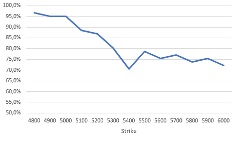
Refer to caption
Fig 2: Ratio of observations satisfying (4.26) as a function of the strike.
Strike 4800 4900 5000 5100 5200 5300 5400 5500 5600 5700 5800 5900 6000
Ratio 96,7% 95,1% 95,1% 88,5% 86,9% 80,3% 70,5% 78,7% 75,4% 77,0% 73,8% 75,4% 72,1%

The results are satisfactory for strikes lower that 5100. Note that when the strike increases less prices’s data are available for the Call option as the strike is too large with respect to the current price SS, see Figure 1. This could explain the degradation of our results.

4.2.2 Super-hedging prices

We test the infimum super-hedging cost deduced from Theorem 4.1 on some data set composed of historical daily closing values of the french index CAC 40 from the 5th of January 2015 to the 12th of March 2018. The interval [0,T][0,T] we choose corresponds to one week composed of 55 working days so that the discrete dates are ti4t^{4}_{i}, i∈{0,⋯,4}i\in\{0,\cdots,4\} and n=4n=4. We first evaluate σti\sigma_{t_{i}}, i∈{0,⋯,3}i\in\{0,\cdots,3\} as

σti=max¯​(|Sti+1Sti−1|/Δ​ti+14,)i∈{0,⋯,3},\displaystyle\sigma_{t_{i}}\>=\overline{\max}\left(\left|\frac{S_{t_{i+1}}}{S_{t_{i}}}-1\right|/\sqrt{\Delta t_{i+1}^{4},}\right)\quad i\in\{0,\cdots,3\}, (4.28)

where max¯\overline{\max} is the empirical maximum taken over a one year sliding sample window of 5252 weeks. Notice that this estimation is model free and does not depend on the strike as it was the case in the preceding sub-section. So we estimate the volatility on 52 weeks and we implement our hedging strategy on the fifty third one. We then repeat the procedure by sliding the window of one week, We observe the empirical average of the stock price S0S_{0} is equal to 40444044.

For a payoff function g⁡(x)=(x−K)+g(x)=(x-K)^{+}, we implement the strategy associated to the super-hedging cost given by Theorem 4.1. The super-hedging cost is given by h⁡(0,S0)h(0,S_{0}) and, using (4.25), we compute the super-hedging strategies (θti4∗)i∈{0,…,3}(\theta_{t_{i}^{4}}^{*})_{i\in\{0,\ldots,3\}}. We denote by VTV_{T} the terminal value of our strategy starting from the minimal price V0=π0,T=h⁡(0,S0)V_{0}=\pi_{0,T}=h(0,S_{0}):

VT=V0+∑i=03θti4∗​Δ​Sti+14.V_{T}=V_{0}+\sum_{i=0}^{3}\theta_{t_{i}^{4}}^{*}\Delta S_{t_{i+1}^{4}}.

We study below the super-hedging error εT=VT−(ST−K)+\varepsilon_{T}=V_{T}-(S_{T}-K)^{+} for different strikes.

Case where K=4700K=4700. The distribution of the super-hedging error εT\varepsilon_{T} for K=4700K=4700 is represented in Figure 3:

Refer to caption
Fig 3: Distribution of the super-hedging error εT=VT−(ST−K)+\varepsilon_{T}=V_{T}-(S_{T}-K)^{+}.

The empirical average of the error εT\varepsilon_{T} is 12.7612.76 and its standard deviation is 21.6521.65. This result is rather satisfactory in comparison to the large value of the empirical mean of S0S_{0} which is equal to 48444844. Notice that we observe E​(ST−K)+≃282.69E(S_{T}-K)^{+}\simeq 282.69. This empirically confirms the efficiency of our suggested method. The empirical probability of {εT<0}\{\varepsilon_{T}<0\} is equal to 14.29%14.29\% but the Value at Risk at 95 % is −10.33-10.33 which confirms that our strategy is conservative.

Refer to caption
Fig 4: Distribution of the ratio V0/S0V_{0}/S_{0}.

The empirical average of V0/S0V_{0}/S_{0} is 5.61%5.61\% and its standard deviation is 5.14%5.14\%. This is again satisfactory since the theoretical super-hedging price in incomplete market is often equal to S0S_{0} (this is for example the case when kd=0k^{d}=0 and ku=∞k^{u}=\infty, in particular when the dynamics of SS is modeled by a (discrete) geometric Brownian motion, see [8]). Note that the loss of -50 is related to so-called black friday week that occures the 24th of June 2016. Large falls of risky assets were observed in European markets mainly explained by the Brexit vote. In particular, the CAC 4040 felt from S0=4340S_{0}=4340 to ST=4106S_{T}=4106, with a loss of −8%-8\% on Friday.

Case where K=S0K=S_{0}. We know present the “at the money” case. The empirical average of the error εT=VT−(ST−K)+\varepsilon_{T}=V_{T}-(S_{T}-K)^{+} is 35.6935.69 and its standard deviation is 34.1134.11. We observe 𝔼⁡(S0)=4844\mathbb{E}(S_{0})=4844, E​(ST−K)+≃38.15E(S_{T}-K)^{+}\simeq 38.15, the probability P⁡(εT<0)=9.82%P(\varepsilon_{T}<0)=9.82\% and the Value at Risk at 95 % is −11.41-11.41. The empirical average of V0/S0V_{0}/S_{0} is 1.51%1.51\% and its standard deviation is 0.47%0.47\%.

Asymmetric case. We now propose another estimation probably more natural of the parameters of the model: ktj−1ndk_{t_{j-1}^{n}}^{d} and ktj−1nuk_{t_{j-1}^{n}}^{u} are estimated as

kti−1nd=min¯​StinSti−1n,kti−1nu=max¯​StinSti−1n,k_{t_{i-1}^{n}}^{d}=\overline{\min}\frac{S_{t_{i}^{n}}}{S_{t_{i-1}^{n}}},\quad k_{t_{i-1}^{n}}^{u}=\overline{\max}\frac{S_{t_{i}^{n}}}{S_{t_{i-1}^{n}}},

where the empirical minimum and maximum are taken over a one year sliding sample window of 5252 weeks, as previously.

Asymmetric case where K=4700K=4700.
The distribution of the super-hedging error εT\varepsilon_{T} for K=4700K=4700 is represented in Figure 5:

Refer to caption
Fig 5: Distribution of the super-hedging error εT=VT−(ST−K)+\varepsilon_{T}=V_{T}-(S_{T}-K)^{+}.

The empirical average of the error εT\varepsilon_{T} is 9.479.47 and its standard deviation is 14.2014.20. This result is rather satisfactory in comparison to the large value of the empirical mean of S0S_{0} which is equal to 48444844. The empirical probability of {εT<0}\{\varepsilon_{T}<0\} is equal to 8.04%8.04\% and the Value at Risk at 95 % is −1.81-1.81 which confirms that our strategy is conservative.

Refer to caption
Fig 6: Distribution of the ratio V0/S0V_{0}/S_{0}.

The empirical average of V0/S0V_{0}/S_{0} is 5.52%5.52\% and its standard deviation is 5.22%5.22\%.

Asymmetric case where K=S0K=S_{0}.

The distribution of the super-hedging error εT\varepsilon_{T} for K=S0K=S_{0} is represented in Figure 7:

Refer to caption
Fig 7: Distribution of the super-hedging error εT\varepsilon_{T}.

The empirical average of the error εT=VT−(ST−K)+\varepsilon_{T}=V_{T}-(S_{T}-K)^{+} is 33.3733.37 and its standard deviation is 32.7832.78. The probability P⁡(εT<0)=12.5%P(\varepsilon_{T}<0)=12.5\%. The Value at Risk at 95 % is −9.29.-9.29.

Refer to caption
Fig 8: Distribution of the ratio V0/S0V_{0}/S_{0}.

The empirical average of V0/S0V_{0}/S_{0} is 1.47%1.47\% and its standard deviation is 0.49%0.49\%.

We now compare the result of both methods is the table below.

Mean of V0/S0V_{0}/S_{0} Variance of V0/S0V_{0}/S_{0} Mean of εT\varepsilon_{T} Variance of εT\varepsilon_{T} P⁡(εT<0)P(\varepsilon_{T}<0) VaR 95 %
Symmetric 5.61% 5.14 % 12.76 21.65 14.29 % -10.33
Asymmetric 5.52% 5.22% 9.47 14.20 8.04% -1.81
Fig 9: Comparison of the two methods of estimation for K=4700K=4700. The mean of S0S_{0} is 4844,93 and the mean of (S0−K)+(S_{0}-K)^{+} is 278,73.
Mean of V0/S0V_{0}/S_{0} Variance of V0/S0V_{0}/S_{0} Mean of εT\varepsilon_{T} Variance of εT\varepsilon_{T} P⁡(εT<0)P(\varepsilon_{T}<0) VaR 95 %
Symmetric 1.51% 0.47 % 35.69 34.11 9.82 % -11.41
Asymmetric 1.47% 0.49% 33.37 32.78 12.50% -9.29
Fig 10: Comparison of the two methods of estimation for K=S0K=S_{0}. The mean of S0S_{0} is 4844,93.

The asymmetric method perform better than the symmetric one which is not a surprise.

5 Appendix

Proof of Corollary 2.10. For all X∈𝒳X\in{\cal X}, ess​supℋ​{h⁡(X),X∈𝒳}≥h⁡(X)\mathrm{ess\,sup}_{{\cal H}}\{h(X),\,X\in{\cal X}\}\geq h(X) a.s. and as ess​supℋ​{h⁡(X),X∈𝒳}\mathrm{ess\,sup}_{{\cal H}}\{h(X),\,X\in{\cal X}\} is ℋ{\cal H}-measurable, we get that a.s.

ess​supℋ​{h⁡(X),X∈𝒳}\displaystyle\mathrm{ess\,sup}_{{\cal H}}\{h(X),\,X\in{\cal X}\} ≥\displaystyle\geq ess​supℋ​h​(X)\displaystyle\mathrm{ess\,sup}_{{\cal H}}h(X)
ess​supℋ​{h⁡(X),X∈𝒳}\displaystyle\mathrm{ess\,sup}_{{\cal H}}\{h(X),\,X\in{\cal X}\} ≥\displaystyle\geq supX∈𝒳ess​supℋ​h​(X).\displaystyle\sup_{X\in{\cal X}}\mathrm{ess\,sup}_{{\cal H}}h(X).

Conversely, for all X∈𝒳X\in{\cal X}, supX∈𝒳ess​supℋ​h​(X)≥h⁡(X)\sup_{X\in{\cal X}}\mathrm{ess\,sup}_{{\cal H}}h(X)\geq h(X) a.s.

If supX∈𝒳ess​supℋ​h​(X)\sup_{X\in{\cal X}}\mathrm{ess\,sup}_{{\cal H}}h(X) is ℋ{\cal H}-measurable, we may conclude that a.s.

supX∈𝒳ess​supℋ​h​(X)≥ess​supℋ​{h⁡(X),X∈𝒳}.\sup_{X\in{\cal X}}\mathrm{ess\,sup}_{{\cal H}}h(X)\geq\mathrm{ess\,sup}_{{\cal H}}\{h(X),\,X\in{\cal X}\}.

Using Proposition 2.9, we get that a.s.

supX∈𝒳ess​supℋ​h​(X)\displaystyle\sup_{X\in{\cal X}}\mathrm{ess\,sup}_{{\cal H}}h(X) =\displaystyle= supX∈𝒳supx∈suppℋ​Xh(x)=supx∈∪X∈𝒳suppℋXh(x).\displaystyle\sup_{X\in{\cal X}}\sup_{x\in\mathrm{supp\,}_{{\cal H}}X}h(x)=\sup_{x\in\cup_{X\in{\cal X}}\mathrm{supp\,}_{{\cal H}}X}h(x).

Since ∪X∈𝒳suppℋX\cup_{X\in{\cal X}}\mathrm{supp\,}_{{\cal H}}X is ℋ{\cal H}-measurable and closed-valued, Lemma 2.12 implies that supx∈∪X∈𝒳suppℋXh(x)\sup_{x\in\cup_{X\in{\cal X}}\mathrm{supp\,}_{{\cal H}}X}h(x) is ℋ{\cal H}-measurable and the proof is complete. □\Box

References

  • [1] Aliprantis, C. D. and K. C. Border. Infinite Dimensional Analysis : A Hitchhicker’s Guide, Grundlehren der Mathematischen Wissenschaften [Fundamental Principles of Mathematical Sciences]. Springer-Verlag, Berlin, 3rd edition, 2006.
  • [2] Baptiste J. and E. Lépinette . Diffusion equations: convergence of the functional scheme derived from the binomial tree with local volatility for non smooth payoff functions. Applied Mathematical Finance, 0,0 (2018), 1-22.
  • [3] Barron E. N., Cardaliaguet, P. and R. Jensen . Conditional Essential Suprema with Applications. Appl Math Optim 48, 229-253, 2003.
  • [4] Barron E. N., and R. Jensen A stochastic control approach to the pricing of options. Mathematics of operations research, 15,1 49-79, 1990.
  • [5] Bensaid B., Lesne J.P., Pagès H. and J. Scheinkman. Derivative asset pricing with transaction costs . Math.Fin. 2, 63-86, 1992.
  • [6] Beiglböck, M. and M. Nutz . Martingale Inequalities and Deterministic Counterparts. Electronic Journal of Probability 19, 95, 1-15, 2014.
  • [7] Bensaid, B., Lesne J.P., Pagès H. and J. Scheinkman. Derivative asset pricing with transaction costs . Math.Fin. 2, 63-86, 1992.
  • [8] Carassus, L., Gobet, E. and E. Temam. A class of financial products and models where super-replication prices are explicit “International Symposium, on Stochastic Processes and Mathematical Finance” at Ritsumeikan University, Kusatsu, Japan, March 2006.
  • [9] Carassus L. and T. Vargiolu. Super-replication price: it can be ok. To appear in ESAIM: proceedings and surveys, 2017.
  • [10] Dalang E.C., Morton A. and W. Willinger. Equivalent martingale measures and no-arbitrage in stochastic securities market models. Stochastics and Stochastic Reports, 29, 185-201, 1990.
  • [11] Delbaen F. and W. Schachermayer. The Mathematics of Arbitrage. Springer Finance, 2006.
  • [12] Föllmer H. and D. Kramkov. Optional Decompositions under Constraints, Probability Theory and Related Fields 109, 1-25, 1997.
  • [13] Harrison J.M. and D.M. Kreps. Martingale and Arbitrage in Multiperiods Securities Markets, Journal of Economic Theory 20, 381-408, 1979.
  • [14] Harrison J.M. and S. Pliska. Martingales and Stochastic Integrals in the Theory of Continuous Trading, Stochastic Processes and their Applications 11, 215-260, 1981.
  • [15] Ingersoll, J.E. Jr. Theory of Financial Decision Making. Rowman & Littlefield, 1987.
  • [16] Hess, C. Set-valued integration and set-valued probability theory: An overview. E. Pap, editor, Handbook of Measure Theory, Elsevier, 14, 617-673, 2002.
  • [17] Kabanov Y. and M. Safarian. Markets with transaction costs. Mathematical Theory. Springer-Verlag, 2009.
  • [18] Kabanov Y. and E. Lépinette. Essential supremum with respect to a random partial order. Journal of Mathematical Economics, 49 , 6, 478-487, 2013.
  • [19] Karatzas I. and C. Kardaras. The numéraire portfolio in semimartingale financial models. Finance & Stochastics, 11, 447-493, 2007.
  • [20] Kreps D. Arbitrage and equilibrium in economies with infinitely many commodities. Journal of Mathematical Economics 8, 15-35, 1981.
  • [21] Lépinette E. and I. Molchanov. Conditional cores and conditional convex hulls of random sets. https://arxiv.org/abs/1711.10303, Preprint 2017.
  • [22] Lépinette E. and T. Tran. Approximate hedging in a local volatility model with proportional transaction costs. Applied Mathematical Finance, 21, 4, 313-341, 2014.
  • [23] Milstein, G.N. The Probability Approach to Numerical Solution of Nonlinear Parabolic Equations. Numerical methods for partial differential equations, 18, 4, 490-522, 2002.
  • [24] Pennanen T. Convex duality in stochastic optimization and mathematical Finance. Mathematics of Operations Research, 36(2), 340-362, 2011.
  • [25] Pennanen T. Arbitrage and Deflators in illiquid markets. Mathematical Finance, 21 pp. 519-540, 2011.
  • [26] Pennanen T. and A-P Perkkio Stochastic programs without duality gaps. Mathematical Programming, 136 pp. 91-110, 2012.
  • [27] Rockafellar, R.T. Convex analysis, Princeton University Press, 1972.
  • [28] R. T. Rockafellar and R. J.-B. Wets. Variational analysis, volume 317 of Grundlehren der Mathematischen Wissenschaften [Fundamental Principles of Mathematical Sciences], 2002. Springer-Verlag, Berlin, 1998. ISBN 3-540-62772-3.
  • [29] Schal M. Martingale measures and hedging for discrete-time financial markets. Mathematics of Operations Research, 24, 509-528, 1999.