Query-Efficient Hard-label Black-box Attack:
An Optimization-based Approach

For simplicity, we consider attacking a $K$-way multi-class classification model in this paper. Given the classification model $f\mathrel{\mathop{\mathchar 58\relax}}\mathbb{R}^{d}\rightarrow\{1,\dots,K\}$ and an original example ${\boldsymbol{x}}_{0}$, the goal is to generate an adversarial example ${\boldsymbol{x}}$ such that

Most attack algorithms in the literature consider the white-box setting, where the classifier $f$ is exposed to the attacker. For neural networks, under this assumption, back-propagation can be conducted on the target model because both network structure and weights are known by the attacker. For classification models in neural networks, it is usually assumed that $f({\boldsymbol{x}})=\operatornamewithlimits{argmax}_{i}(Z({\boldsymbol{x}})_{i})$, where $Z({\boldsymbol{x}})\in\mathbb{R}^{K}$ is the final (logit) layer output, and $Z({\boldsymbol{x}})_{i}$ is the prediction score for the $i$-th class. The objectives in (1) can then be naturally formulated as the following optimization problem:

where $\text{Dis}(\cdot,\cdot)$ is some distance measurement (e.g., $\ell_{2},\ell_{1}$ or $\ell_{\infty}$ norm in Euclidean space), $\mathscr{L}(\cdot)$ is the loss function corresponding to the goal of the attack, and $c$ is a balancing parameter. For untargeted attack, where the goal is to make the target classifier misclassify, the loss function can be defined as

where $y_{0}$ is the original label predicted by the classifier. For targeted attack, where the goal is to turn it into a specific target class $t$, the loss function can also be defined accordingly.

Therefore, attacking a machine learning model can be posed as solving this optimization problem [9, 12], which is also known as the C&W attack or the EAD attack depending on the choice of the distance measurement. To solve (2), one can apply any gradient-based optimization algorithm such as SGD or Adam, since the gradient of $\mathscr{L}(Z({\boldsymbol{x}}))$ can be computed via back-propagation.

The ability of computing gradient also enables many different attacks in the white-box setting. For example, eq (2) can also be turned into a constrained optimization problem, which can then be solved by projected gradient descent (PGD) [11]. FGSM [3] is the special case of one step PGD with $\ell_{\infty}$ norm distance. Other algorithms such as Deepfool [6] also solve similar optimization problems to construct adversarial examples.

In real-world systems, usually the underlying machine learning model will not be revealed and thus white-box attacks cannot be applied. This motivates the study of attacking machine learning models in the black-box setting, where attackers do not have any information about the function $f$. And the only valid operation is to make queries to the model and get the corresponding output $f({\boldsymbol{x}})$. The first approach for black-box attack is using transfer attack [14]—instead of attacking the original model $f$, attackers try to construct a substitute model $\hat{f}$ to mimic $f$ and then attack $\hat{f}$ using white-box attack methods. This approach has been well studied and analyzed in [15]. However, recent papers have shown that attacking the substitute model usually leads to much larger distortion and low success rate [10]. Therefore, instead, [10] considers the score-based black-box setting, where attackers can use ${\boldsymbol{x}}$ to query the softmax layer output in addition to the final classification result. In this case, they can reconstruct the loss function (3) and evaluate it as long as the objective function $h({\boldsymbol{x}})$ exists for any ${\boldsymbol{x}}$. Thus a zeroth order optimization approach can be directly applied to minimize $h({\boldsymbol{x}})$. [16] further improves the query complexity of [10] by introducing two novel building blocks: (i) an adaptive random gradient estimation algorithm that balances query counts and distortion, and (ii) a well-trained autoencoder that achieves attack acceleration. [13] also solves a score-based attack problem using an evolutionary algorithm and it shows their method could be applied to hard-label black-box setting as well.

Throughout this paper, the hard-label black-box setting refers to cases where real-world ML systems only provide limited prediction results of an input query. Specifically, only the final decision (top-1 predicted label) instead of probability outputs is known to an attacker.

Attacking in this setting is very challenging. In Figure 1a, we show a simple 3-layer neural network’s decision boundary. Note that the $\mathscr{L}(Z({\boldsymbol{x}}))$ term is continuous as in Figure 1b because the logit layer output is real-valued functions. However, in the hard-label black-box setting, only $f(\cdot)$ is available instead of $Z(\cdot)$. Since $f(\cdot)$ can only be one-hot vector, if we plug-in $f$ into the loss function, $\mathscr{L}(f({\boldsymbol{x}}))$ (as shown in Figure 1c) will be discontinuous and with discrete outputs.

Optimizing this function will require combinatorial optimization or search algorithms, which is almost impossible to do given high dimensionality of the problem. Therefore, almost no algorithm can successfully conduct hard-label black-box attack in the literature. The only current approach [1] is based on random-walk on the boundary. Although this decision-based attack can find adversarial examples with comparable distortion with white-box attacks, it suffers from exponential search time, resulting in lots of queries, and lacks convergence guarantees. We show that our optimization-based algorithm can significantly reduce the number of queries compared with decision-based attack, and has guaranteed convergence in the number of iterations (queries).

For a given example ${\boldsymbol{x}}_{0}$, true label $y_{0}$ and the hard-label black-box function $f\mathrel{\mathop{\mathchar 58\relax}}\mathbb{R}^{d}\rightarrow\{1,\dots,K\}$, we define our objective function $g\mathrel{\mathop{\mathchar 58\relax}}\mathbb{R}^{d}\rightarrow\mathbb{R}$ depending on the type of attack:

In this formulation, ${\boldsymbol{\theta}}$ represents the search direction and $g({\boldsymbol{\theta}})$ is the distance from ${\boldsymbol{x}}_{0}$ to the nearest adversarial example along the direction ${\boldsymbol{\theta}}$. The difference between (4) and (5) corresponds to the different definitions of “successfulness” in untargeted and targeted attack, where the former one aims to turn the prediction into any incorrect label and the later one aims to turn the prediction into the target label. For untargeted attack, $g({\boldsymbol{\theta}})$ also corresponds to the distance to the decision boundary along the direction ${\boldsymbol{\theta}}$. In image problems the input domain of $f$ is bounded, so we will add corresponding upper/lower bounds in the definition of (4) and (5).

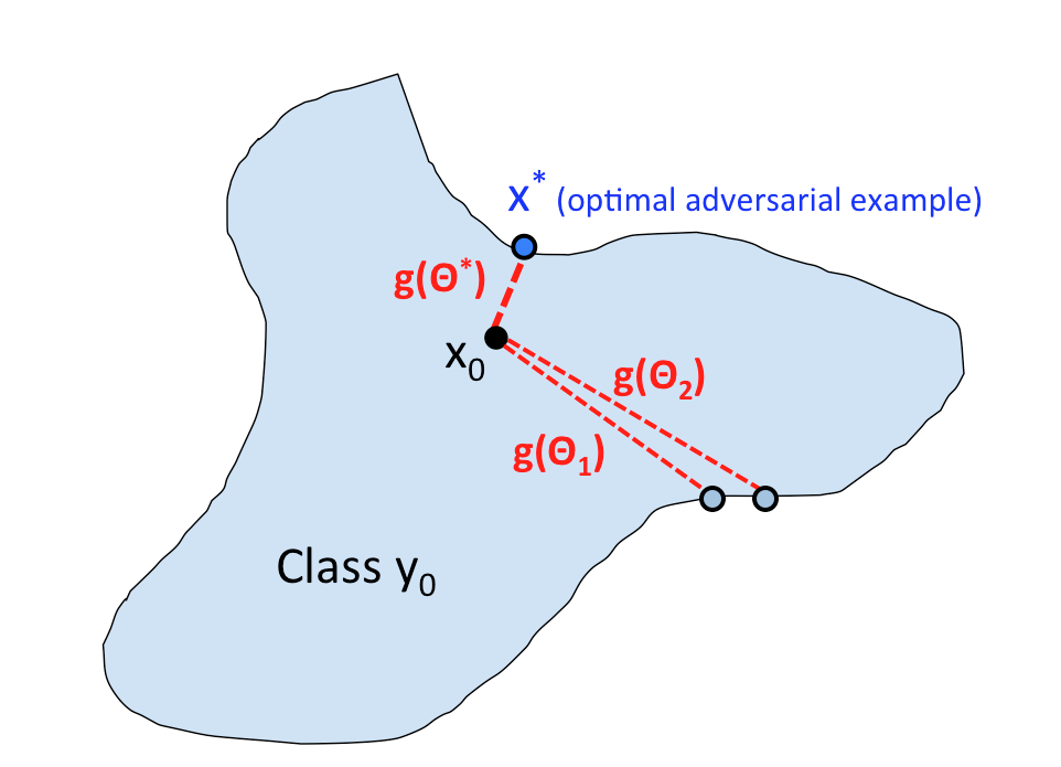
Instead of searching for an adversarial example, we search the direction ${\boldsymbol{\theta}}$ to minimize the distortion $g({\boldsymbol{\theta}})$, which leads to the following optimization problem:

Finally, the adversarial example can be found by ${\boldsymbol{x}}^{*}={\boldsymbol{x}}_{0}+g({\boldsymbol{\theta}}^{*})\frac{{\boldsymbol{\theta}}^{*}}{\|{\boldsymbol{\theta}}^{*}\|}$, where ${\boldsymbol{\theta}}^{*}$ is the optimal solution of (6).

Note that unlike the C&W or PGD objective functions, which are discontinuous step functions in the hard-label setting (see Section 2), $g({\boldsymbol{\theta}})$ maps input direction to real-valued output (distance to decision boundary), which is usually continuous—a small change of ${\boldsymbol{\theta}}$ usually leads to a small change of $g({\boldsymbol{\theta}})$, as can be seen from Figure 2.

Moreover, we give three examples of $f({\boldsymbol{x}})$ defined in two dimension input space and their corresponding $g({\boldsymbol{\theta}})$. In Figure  3a, we have a continuous classification function defined as follows

In this case, as shown in Figure  3c, $g({\boldsymbol{\theta}})$ is continuous. Moreover, in Figure  3b and Figure  1a, we show decision boundaries generated by GBDT and neural network classifier, which are not continuous. However, as showed in Figure  3d and Figure  1d, even if the classifier function is not continuous, $g({\boldsymbol{\theta}})$ is still continuous. This makes it easy to apply zeroth order method to solve (6).

Compute $g({\boldsymbol{\theta}})$ up to certain accuracy. We are not able to evaluate the gradient of $g$, but we can evaluate the function value of $g$ using the hard-label queries to the original function $f$. For simplicity, we focus on untargeted attack here, but the same procedure can be applied to targeted attack as well.

First, we discuss how to compute $g({\boldsymbol{\theta}})$ directly without additional information. This is used in the initialization step of our algorithm. For a given normalized ${\boldsymbol{\theta}}$, we do a fine-grained search and then a binary search. In fine-grained search, we query the points $\{{\boldsymbol{x}}_{0}+\alpha{\boldsymbol{\theta}},{\boldsymbol{x}}_{0}+2\alpha{\boldsymbol{\theta}},\dots\}$ one by one until we find $f({\boldsymbol{x}}+i\alpha{\boldsymbol{\theta}})\neq y_{0}$. This means the boundary goes between $[{\boldsymbol{x}}_{0}+(i-1)\alpha{\boldsymbol{\theta}},{\boldsymbol{x}}_{0}+i\alpha{\boldsymbol{\theta}}]$. We then enter the second phase and conduct a binary search to find the solution within this region (same with line 11–17 in Algorithm 1). Note that there is an upper bound of the first stage if we choose ${\boldsymbol{\theta}}$ by the direction of ${\boldsymbol{x}}-{\boldsymbol{x}}_{0}$ with some ${\boldsymbol{x}}$ from another class. This procedure is used to find the initial ${\boldsymbol{\theta}}_{0}$ and corresponding $g({\boldsymbol{\theta}}_{0})$ in our optimization algorithm. We omit the detailed algorithm for this part since it is similar to Algorithm 1.

Next, we discuss how to compute $g({\boldsymbol{\theta}})$ when we know the solution is very close to a value $v$. This is used in all the function evaluations in our optimization algorithm, since the current solution is usually close to the previous solution, and when we estimate the gradient using (7), the queried direction will only be a small perturbation of the previous one. In this case, we first increase or decrease $v$ in local region to find the interval that contains boundary (e.g, $f(v)=y_{0}$ and $f(v^{\prime})\neq y_{0}$), then conduct a binary search to find the final value of $g$. Our procedure for computing $g$ value is presented in Algorithm 1.

To solve the optimization problem (1) for which we can only evaluate function value instead of gradient, zeroth order optimization algorithms can be naturally applied. In fact, after the reformulation, the problem can be potentially solved by any zeroth order optimization algorithm, like zeroth order gradient descent or coordinate descent (see [17] for a comprehensive survey).

Here we propose to solve (1) using Randomized Gradient-Free (RGF) method proposed in [2, 18]. In practice we found it outperforms zeroth-order coordinate descent. In each iteration, the gradient is estimated by

where ${\boldsymbol{u}}$ is a random Gaussian vector, and $\beta>0$ is a smoothing parameter (we set $\beta=0.005$ in all our experiments). The solution is then updated by ${\boldsymbol{\theta}}\leftarrow{\boldsymbol{\theta}}-\eta\hat{{\boldsymbol{g}}}$ with a step size $\eta$. The procedure is summarized in Algorithm 2.

There are several implementation details when we apply this algorithm. First, for high-dimensional problems, we found the estimation in (7) is very noisy. Therefore, instead of using one vector, we sample $q$ vectors from Gaussian distribution and average their estimators to get $\hat{{\boldsymbol{g}}}$. We set $q=20$ in all the experiments. The convergence proofs can be naturally extended to this case. Second, instead of using a fixed step size (suggested in theory), we use a backtracking line-search approach to find step size at each step. This leads to additional query counts, but makes the algorithm more stable and eliminates the need to hand-tuning the step size.

If $g({\boldsymbol{\theta}})$ can be computed exactly, it has been proved in [2] that RGF in Algorithm 2 requires at most $O(\frac{d}{\delta^{2}})$ iterations to converge to a point with $\|\nabla g({\boldsymbol{\theta}})\|^{2}\leq\delta^{2}$. However, in our algorithm the function value $g({\boldsymbol{\theta}})$ cannot be computed exactly; instead, we compute it up to $\epsilon$-precision, and this precision can be controlled by binary threshold in Algorithm 1. We thus extend the proof in [2] to include the case of approximate function value evaluation, as described in the following theorem.

Detailed proofs can be found in the appendix. Note that the binary search procedure could obtain the desired function value precision in $O(\log\delta)$ steps. By using the same idea with Theorem 1 and following the proof in [2], we could also achieve $O(\frac{d^{2}}{\delta^{3}})$ complexity when $g({\boldsymbol{\theta}})$ is non-smooth but Lipschitz continuous.

We use three standard datasets: MNIST [19], CIFAR-10 [20] and ImageNet-1000 [21]. To have a fair comparison with previous work, we adopt the same networks used in both  [9] and  [1]. In detail, both MNIST and CIFAR use the same network structure with four convolution layers, two max-pooling layers and two fully-connected layers. Using the parameters provided by  [9], we could achieve 99.5% accuracy on MNIST and 82.5% accuracy on CIFAR-10, which is similar to what was reported in  [9]. For Imagenet-1000, we use the pretrained network Resnet-50  [22] provided by torchvision¹¹ 1 https://github.com/pytorch/vision/tree/master/torchvision, which could achieve 76.15% top-1 accuracy. All models are trained using Pytorch and our source code is publicly available²² 2 https://github.com/LeMinhThong/blackbox-attack.

We include the following algorithms into comparison:

• •

  Opt-based black-box attack (Opt-attack): our proposed algorithm.

• •

  Decision-based black-box attack [1] (Decision-attack): the only previous work on attacking hard-label black box model. We use the authors’ implementation and use default parameters provided in Foolbox³³ 3 https://github.com/bethgelab/foolbox.

• •

  C&W white-box attack [9]: one of the current state-of-the-art attacking algorithm in the white-box setting. We do binary search on parameter $c$ per image to achieve the best performance. Attacking in the white-box setting is a much easier problem, so we include C&W attack just for reference and indicate the best performance we can possibly achieve.

For all the cases, we conduct adversarial attacks for randomly sampled $N=100$ images from validation sets. Note that all three attacks have 100% successful rate, and we report the average $L_{2}$ distortion, defined by $\frac{1}{N}\sum_{i=1}^{N}\|{\boldsymbol{x}}^{(i)}-{\boldsymbol{x}}_{0}^{(i)}\|_{2}$, where ${\boldsymbol{x}}^{(i)}$ is the adversarial example constructed by an attack algorithm and ${\boldsymbol{x}}_{0}^{(i)}$ is the original $i$-th example. For black-box attack algorithms, we also report average number of queries for comparison.

Suppose $g$ has a lipschitz-continuous gradient with constant $L_{1}(g)$, then

We could bound $E_{u}(||\hat{g}({\boldsymbol{\theta}})||^{2})$ as follows. Since

and $|\epsilon_{{\boldsymbol{\theta}}+\beta u}-\epsilon_{{\boldsymbol{\theta}}}|\leq 2\epsilon$,

Take expectation over u, and with Theorem 3 in  [24], which is $E_{u}(||g^{\prime}({\boldsymbol{\theta}},u)\cdot u||^{2})\leq(d+4)||\nabla g(x)||^{2}$,

With $\epsilon\sim O(\delta^{2}\beta)$, we could bound $E_{u}(||\tilde{g}({\boldsymbol{\theta}})||^{2})$:

We use the result that

which is proved in  [24] Lemma 4.

Therefore, since $(n+6)^{3}+2(n+4)^{3}\leq 3(n+5)^{3}$, we could get

Therefore, since $g_{\beta}({\boldsymbol{\theta}})$ has Lipshcitz-continuous gradient:

so that

Since

where $\mathbb{1}$ is a all-one vector, taking the expectation in $u_{k}$, we obtain

Choosing $\alpha_{k}=\hat{\alpha}=\frac{1}{4(d+4)L_{1}(f)}$, we obtain

Since $(d+5)^{3}\leq(d+8)(d+4)^{2}$, taking expectation over $\mathscr{U}_{k}$, where $\mathscr{U}_{k}=\{u_{1},u_{2},\dots,u_{k}\}$, we get

where $\phi_{k}=E_{\mathscr{U}_{k-1}(g({\boldsymbol{\theta}}_{k}))},k\geq 1$ and $\phi_{0}=g({\boldsymbol{\theta}}_{0})$.

Assuming $g(x)\geq g^{*}$, summing over k and divided by N+1, we get

Clearly, $\frac{1}{N+1}\sum\limits_{k=0}^{N}E_{\mathscr{U}_{k}}(||\nabla g_{\beta}({\boldsymbol{\theta}}_{k})||)\leq\delta^{2}$.

Since $\vartheta_{k}^{2}=E_{\mathscr{U}_{k}}(||\nabla g({\boldsymbol{\theta}}_{k})||^{2})\leq 2E_{\mathscr{U}_{k}}(||\nabla g_{\beta}({\boldsymbol{\theta}}_{k})||^{2})+\frac{\beta^{2}(d+4)^{2}}{2}L_{1}^{2}(g)$, $\vartheta_{k}^{2}$ is in the same order oas$E_{\mathscr{U}_{k}}(||\nabla g_{\beta}({\boldsymbol{\theta}}_{k})||^{2})$. In order to satisfy $\frac{1}{N+1}\sum\limits_{k=0}^{N}\vartheta_{k}^{2}\leq\delta^{2}$, we need to choose $\beta\leq O(\frac{\delta}{dL_{1}(g)})$, then N is bounded by $O(\frac{d}{\delta^{2}})$.

References

- [1] Wieland Brendel, Jonas Rauber, and Matthias Bethge. Decision-based adversarial attacks: Reliable attacks against black-box machine learning models. arXiv preprint arXiv:1712.04248, 2017.
- [2] Yurii Nesterov and Vladimir Spokoiny. Random gradient-free minimization of convex functions. Foundations of Computational Mathematics, 17(2):527–566, 2017.
- [3] Ian J Goodfellow, Jonathon Shlens, and Christian Szegedy. Explaining and harnessing adversarial examples. arXiv preprint arXiv:1412.6572, 2014.
- [4] Christian Szegedy, Wojciech Zaremba, Ilya Sutskever, Joan Bruna, Dumitru Erhan, Ian Goodfellow, and Rob Fergus. Intriguing properties of neural networks. arXiv preprint arXiv:1312.6199, 2013.
- [5] Seyed-Mohsen Moosavi-Dezfooli, Alhussein Fawzi, Omar Fawzi, and Pascal Frossard. Universal adversarial perturbations.
- [6] Seyed Mohsen Moosavi Dezfooli, Alhussein Fawzi, and Pascal Frossard. Deepfool: a simple and accurate method to fool deep neural networks. In Proceedings of 2016 IEEE Conference on Computer Vision and Pattern Recognition (CVPR), number EPFL-CONF-218057, 2016.
- [7] Hongge Chen, Huan Zhang, Pin-Yu Chen, Jinfeng Yi, and Cho-Jui Hsieh. Attacking visual language grounding with adversarial examples: A case study on neural image captioning. In ACL, 2018.
- [8] Minhao Cheng, Jinfeng Yi, Huan Zhang, Pin-Yu Chen, and Cho-Jui Hsieh. Seq2sick: Evaluating the robustness of sequence-to-sequence models with adversarial examples. CoRR, 2018.
- [9] Nicholas Carlini and David Wagner. Towards evaluating the robustness of neural networks. In Security and Privacy (SP), 2017 IEEE Symposium on, pages 39–57. IEEE, 2017.
- [10] Pin-Yu Chen, Huan Zhang, Yash Sharma, Jinfeng Yi, and Cho-Jui Hsieh. Zoo: Zeroth order optimization based black-box attacks to deep neural networks without training substitute models. In Proceedings of the 10th ACM Workshop on Artificial Intelligence and Security, pages 15–26. ACM, 2017.
- [11] Aleksander Madry, Aleksandar Makelov, Ludwig Schmidt, Dimitris Tsipras, and Adrian Vladu. Towards deep learning models resistant to adversarial attacks. In ICLR, 2018.
- [12] Pin-Yu Chen, Yash Sharma, Huan Zhang, Jinfeng Yi, and Cho-Jui Hsieh. Ead: elastic-net attacks to deep neural networks via adversarial examples. In AAAI, 2018.
- [13] Andrew Ilyas, Logan Engstrom, Anish Athalye, and Jessy Lin. Query-efficient black-box adversarial examples. arXiv preprint arXiv:1712.07113, 2017.
- [14] Nicolas Papernot, Patrick McDaniel, Ian Goodfellow, Somesh Jha, Z Berkay Celik, and Ananthram Swami. Practical black-box attacks against machine learning. In Proceedings of the 2017 ACM on Asia Conference on Computer and Communications Security, pages 506–519. ACM, 2017.
- [15] Arjun Nitin Bhagoji, Warren He, Bo Li, and Dawn Song. Exploring the space of black-box attacks on deep neural networks. arXiv preprint arXiv:1712.09491, 2017.
- [16] Chun-Chen Tu, Pai-Shun Ting, Pin-Yu Chen, Sijia Liu, Huan Zhang, Jinfeng Yi, Cho-Jui Hsieh, and Shin-Ming Cheng. Autozoom: Autoencoder-based zeroth order optimization method for attacking black-box neural networks. CoRR, abs/1805.11770, 2018.
- [17] Andrew R Conn, Katya Scheinberg, and Luis N Vicente. Introduction to derivative-free optimization, volume 8. Siam, 2009.
- [18] Saeed Ghadimi and Guanghui Lan. Stochastic first-and zeroth-order methods for nonconvex stochastic programming. SIAM Journal on Optimization, 23(4):2341–2368, 2013.
- [19] Yann LeCun, Léon Bottou, Yoshua Bengio, and Patrick Haffner. Gradient-based learning applied to document recognition. Proceedings of the IEEE, 86(11):2278–2324, 1998.
- [20] Alex Krizhevsky. Learning multiple layers of features from tiny images. 2009.
- [21] Jia Deng, Wei Dong, Richard Socher, Li-Jia Li, Kai Li, and Li Fei-Fei. Imagenet: A large-scale hierarchical image database. In Computer Vision and Pattern Recognition, 2009. CVPR 2009. IEEE Conference on, pages 248–255. IEEE, 2009.
- [22] Kaiming He, Xiangyu Zhang, Shaoqing Ren, and Jian Sun. Deep residual learning for image recognition. In Proceedings of the IEEE conference on computer vision and pattern recognition, pages 770–778, 2016.
- [23] Pierre Baldi, Peter Sadowski, and Daniel Whiteson. Searching for exotic particles in high-energy physics with deep learning. Nature communications, 5:4308, 2014.
- [24] Yurii Nesterov. Random gradient-free minimization of convex functions. Technical report, 2011.
6 Appendix
Because there is a stopping criterion in Algorithm 1, we couldn’t achieve the exact . Instead, we could get with error, i.e., . Also, we define to be the noisy gradient estimator.
Following [24], we define the Guassian smoothing approximation over , i.e,