Spherical surfaces with conical points: systole inequality and moduli spaces with many connected components

Gabriele Mondello Affiliation: “Sapienza” Università di Roma, Department of Mathematics (mondello@mat.uniroma1.it) Dmitri Panov Affiliation: King’s College London, Department of Mathematics (dmitri.panov@kcl.ac.uk)

Abstract

In this article we address a number of features of the moduli space of spherical metrics on connected, compact, orientable surfaces with conical singularities of assigned angles, such as its non-emptiness and connectedness. We also consider some features of the forgetful map from the above moduli space of spherical surfaces with conical points to the associated moduli space of pointed Riemann surfaces, such as its properness, which follows from an explicit systole inequality that relates metric invariants (spherical systole) and conformal invariant (extremal systole).

1 Introduction

The aim of the present paper is to investigate certain topological properties of the moduli space $\text{\footnotesize{$\mathpzc{MSph}$}}_{g,n}(\text{\boldmath$\vartheta$})$ of spherical metrics on genus $g$ surfaces with $n$ conical singularities of angles $2\pi\cdot\text{\boldmath$\vartheta$}=2\pi\cdot(\vartheta_{1},\dots,\vartheta_{n})$ , and of the associated forgetful map $F_{g,n,\text{\boldmath$\vartheta$}}:\text{\footnotesize{$\mathpzc{MSph}$}}_{g,n}(\text{\boldmath$\vartheta$})\rightarrow\text{\footnotesize{$\mathpzc{M}$}}_{g,n}$ that sends a spherical surface to its underlying Riemann surface of genus $g$ with $n$ marked points.

Our main results, labeled as Theorems A-B-C-D-E, can be summarized as follows:

(A)

$\text{\footnotesize{$\mathpzc{MSph}$}}_{g,n}(\text{\boldmath$\vartheta$})$ is always non-empty for $g>0$ , provided the obvious Gauss-Bonnet constraint is satisfied;
(B)

for suitable $\vartheta$ , the moduli space $\text{\footnotesize{$\mathpzc{MSph}$}}_{0,3+m}(\text{\boldmath$\vartheta$})$ and its image through the forgetful map $F_{0,3+m,\text{\boldmath$\vartheta$}}$ have at least $3^{m}$ connected components;
(C)

if $\vartheta$ does not belong to a certain well-understood locally finite union of affine hyperplanes of $\mathbb{R}^{n}$ (at which some bubbling phenomenon can occur), spherical systole and extremal systole of spherical surfaces in $\text{\footnotesize{$\mathpzc{MSph}$}}_{g,n}(\text{\boldmath$\vartheta$})$ bound each other through an explicit systole inequality;
(D)

for every $(g,n)\neq(0,2),\,(0,3)$ with $n\geq 2$ and for every fixed conformal class there exists an open subset of $\text{\boldmath$\vartheta$}\in\mathbb{R}_{>0}^{n}$ such that $\text{\footnotesize{$\mathpzc{MSph}$}}_{g,n}(\text{\boldmath$\vartheta$})$ is non-empty but it contains no metric in the given conformal class; moreover, the $\vartheta$ ’s occurring in such open subset can have arbitrarily small $\vartheta_{1}$ ;
(E)

under the same (non-bubbling) hypotheses of Theorem C, the forgetful map $F_{g,n,\text{\boldmath$\vartheta$}}$ is proper.

Complete statements can be found in Subsection 1.2.

We remark that Theorems C-D-E are genus independent.

On the contrary, Theorem A only holds for positive genus and it is false in genus zero, since the simple topology of the sphere imposes some constraints on the possible monodromy representation of a spherical metric (see Subsection 1.3.5).

The content of Theorem B is essentially to provide examples of moduli spaces with many connected components. Our construction works in genus zero because $\text{\footnotesize{$\mathpzc{MSph}$}}_{0,3}\left(\frac{1}{2}+m_{1},\frac{1}{2}+m_{2},\frac{1}{2}+m_{3}\right)$ consists of a single point for $m_{1},m_{2},m_{3}\in\mathbb{Z}_{\geq 0}$ , and because such a point represents a spherical surface with discrete (and so finite) monodromy. The study of such phenomena of disconnectedness in higher genus is object of future work.

Theorems stated in Subsection 1.3, which are not labeled by letters, are extracted from previous works of various authors.

1.1 Setting

In this subsection we introduce the notion of spherical surface with conical points, of (metric) systole and of extremal systole, and of non-bubbling parameter. Moreover, we recall the definition of forgetful map from the moduli space of spherical surfaces with conical points to the moduli space of Riemann surfaces with marked points.

Let $S$ be a compact, connected, oriented surface and let $\dot{S}$ be the punctured surface obtained from $S$ by removing a subset $\text{\boldmath$x$}=(x_{1},\dots,x_{n})$ of $n$ marked points.

A metric of curvature $1$ on a surface is locally isometric to $\mathbb{S}^{2}$ and so it can be locally written as $d\rho^{2}+\sin^{2}(\rho)d\phi^{2}$ in polar coordinates $(\rho,\phi)$ . The model for a closed neighborhood of a conical point of angle $2\pi\theta$ inside a spherical surface will be the disk $\mathbb{D}_{\theta}(r)=\{z=\rho e^{i\phi}\in\mathbb{C}\,|\,|z|\leq r\}$ with $0<r<\pi$ , endowed with the metric $d\rho^{2}+\theta^{2}\sin^{2}(\rho)d\phi^{2}$ .

Definition 1.1 (Spherical metric).

A spherical metric on $S$ with conical singularities at $x$ of angles $2\pi\text{\boldmath$\vartheta$}=2\pi(\vartheta_{1},\dots,\vartheta_{n})$ is a Riemannian metric $h$ of curvature $1$ on $\dot{S}$ such that every $x_{i}$ has a closed neighbourhood isometric to $\mathbb{D}_{\vartheta_{i}}(r)$ for some small $r>0$ . We will call $(S,\text{\boldmath$x$},h)$ a spherical surface and each $x_{i}$ a conical point.

Remark 1.2 (Developing map and monodromy representation).

For every spherical surface $(S,\text{\boldmath$x$},h)$ we can construct a locally isometric developing map $\iota:(\widetilde{\dot{S}},\tilde{h})\rightarrow\mathbb{S}^{2}$ from the universal cover $\widetilde{\dot{S}}$ of $\dot{S}$ (endowed with the pull-back metric $\tilde{h}$ ), which is equivariant with respect to a monodromy representation $\rho:\pi_{1}(\dot{S})\rightarrow\mathrm{SO}_{3}(\mathbb{R})$ . The couple $(\iota,\rho)$ is well-defined up to the action $\mathcal{Q}\cdot(\iota,\rho)=(\mathcal{Q}\circ\iota,\mathcal{Q}\rho\mathcal{Q}^{-1})$ by elements $\mathcal{Q}\in\mathrm{SO}_{3}(\mathbb{R})$ .

Each spherical surface $(S,h)$ admits a triangulation, where all edges are geodesic segments and all triangles are isometric to spherical triangles with respect to the induced metric $h$ . In other words, each spherical surface is a polyhedral space (see [29, Section 8] for a nice introduction to the topic). In this description all conical points sit at some vertices of the triangulation.

Notation.

If $p\in S$ is any point in the spherical surface $S$ and $r>0$ , we denote by $B_{p}(r)$ the closed ball centered at $p$ of radius $r$ , namely the locus of points at distance at most $r$ from $p$ .

The diameter of a spherical surface with $n$ conical points is at most $\pi(n+1)$ (see Lemma 3.2). For this reason, a sequence of spherical metrics degenerates if and only if two (or more) conical points clash or if a geodesic loop based at a conical point shrinks to a singular point. Thus, the following quantity can be interpreted as a measure of how far the metric is from degenerating.

Definition 1.3 (Spherical systole).

The systole $\mathrm{sys}(S,\text{\boldmath$x$})$ of a spherical surface $(S,\text{\boldmath$x$})$ is the supremum of all $r>0$ for which the $n$ balls $B_{x_{i}}(r)$ are pairwise disjoint and each $B_{x_{i}}(r)$ is isometric to $\mathbb{D}_{\vartheta_{i}}(r)$ .

We recall that the datum of a conformal class of metrics on an oriented surface $S$ is equivalent to giving an almost-complex structure $J:TS\rightarrow TS$ , and so to giving a complex structure by Gauss’s existence of isothermal coordinates. In what follows, we will denote a Riemann surface by $(S,J)$ .

The conformal counterpart to the spherical systole, which measures how far the underlying conformal structure on a surface is from degenerating, is introduced in Definition 1.4 below. The definition and some basic properties of the extremal length and of the conformal modulus of a cylinder are summarized in Appendix A.

Definition 1.4 (Extremal systole).

Let $(S,J)$ be a Riemann surface with marked points $x$ and assume that $\dot{S}$ is not a sphere with at most $3$ punctures. The extremal systole $\mathrm{Ext}\mathrm{sys}(\dot{S})$ of $\dot{S}$ is the infimum of the extremal lengths $\mathrm{Ext}_{\gamma}(\dot{S})$ , where $\gamma\subset\dot{S}$ is a simple closed essential curve.

We will use the notation $\mathrm{Ext}\mathrm{sys}(\dot{S},J)$ whenever we want to emphasize the dependence on $J$ . Clearly, if $(S,\text{\boldmath$x$})$ is a spherical surface, then $\mathrm{Ext}\mathrm{sys}(\dot{S})$ must be understood as the extremal systole of the underlying conformal structure.

Next, we introduce a quantity that depends only on the topology of $(S,\text{\boldmath$x$})$ and on the angle vector $\vartheta$ . Consider the subset $\mathrm{Crit}_{\text{\boldmath$\vartheta$}}\subset\mathbb{R}$ defined as

\mathrm{Crit}_{\text{\boldmath$\vartheta$}}:=\left\{\|\text{\boldmath$\vartheta$}_{I}\|_{1}-\|\text{\boldmath$\vartheta$}_{I^{c}}\|_{1}+2b\ \Big|\ I\subsetneq\{1,2,\dots,n\},\ b\in\mathbb{Z}_{\geq 0}\right\}

where $\|\text{\boldmath$\vartheta$}_{I}\|_{1}:=\sum_{i\in I}\vartheta_{i}$ and $I^{c}=\{1,2,\dots,n\}\setminus I$ .

Definition 1.5 (Non-bubbling parameter).

The non-bubbling parameter of $(S,\text{\boldmath$x$},\text{\boldmath$\vartheta$})$ is

\mathrm{NB}_{\text{\boldmath$\vartheta$}}(S,\text{\boldmath$x$}):=d_{\mathbb{R}}\Big(\chi(\dot{S}),\mathrm{Crit}_{\text{\boldmath$\vartheta$}}\Big)

where $d_{\mathbb{R}}$ is the usual distance as subsets of $\mathbb{R}$ .

Remark 1.6.

We stress that

\mathrm{NB}_{\text{\boldmath$\vartheta$}}(S,\text{\boldmath$x$})=0\iff\chi(\dot{S})+\sum_{i=1}^{n}(\pm\vartheta_{i})\in 2\mathbb{Z}_{\geq 0}

for a suitable choice of the signs.

We will explain in Section 1.3.3 that the condition $\mathrm{NB}_{\text{\boldmath$\vartheta$}}(S,\text{\boldmath$x$})\geq\varepsilon$ prevents spherical metrics on $(S,\text{\boldmath$x$})$ with conical angles $2\pi\text{\boldmath$\vartheta$}$ from being geometrically close to a bouquet of bubbles (as in Figure 1.3.3).

Another feature of the non-bubbling parameter is that it provides an obstruction for spherical surfaces to having degenerate monodromy representation in the following sense.

Definition 1.7 (Coaxial representation).

A representation $\rho$ in $\mathrm{SO}_{3}(\mathbb{R})$ is coaxial if it takes values in a $1$ -parameter subgroup of $\mathrm{SO}_{3}(\mathbb{R})$ . We say that a metric has coaxial monodromy (or that it is a coaxial metric) if its monodromy representation is coaxial.

The link between non-bubbling parameter and coaxiality is the following.

Lemma 9.3 (Coaxial metrics have vanishing non-bubbling parameter).

Let $(S,\text{\boldmath$x$})$ be a spherical surface with conical points of angles $2\pi\cdot\text{\boldmath$\vartheta$}$ . If $(S,\text{\boldmath$x$})$ has coaxial monodromy, then $\mathrm{NB}_{\text{\boldmath$\vartheta$}}(S,\text{\boldmath$x$})=0$ .

The above lemma can be proven in more than one way. In Section 9 we will derive it from Theorem C.

Notation.

Since $\mathrm{NB}_{\text{\boldmath$\vartheta$}}(S,\text{\boldmath$x$})$ only depends on $\vartheta$ and on the topology of the surface $S$ of genus $g$ with $n$ marked points, such quantity will be also denoted by $\mathrm{NB}_{\text{\boldmath$\vartheta$}}(g,n)$ .

Finally, we recall the definition of moduli spaces of Riemann surfaces and of spherical surfaces.

Definition 1.8 (Moduli space of Riemann surfaces).

Let $g,n\geq 0$ with $2g-2+n>0$ . The moduli space $\text{\footnotesize{$\mathpzc{M}$}}_{g,n}$ of Riemann surfaces of genus $g$ with $n$ marked points is the space of isomorphism classes $[S,\text{\boldmath$x$},J]$ , where $J$ is a complex structure on the connected oriented surface $S$ of genus $g$ and $\text{\boldmath$x$}=(x_{1},\dots,x_{n})$ is a collection of $n$ distinct points on $S$ .

We recall that $\text{\footnotesize{$\mathpzc{M}$}}_{g,n}$ is a complex-analytic connected orbifold of complex dimension $3g-3+n$ .

Definition 1.9 (Moduli space of spherical surfaces).

Let $g,n\geq 0$ with $2g-2+n>0$ and let $\text{\boldmath$\vartheta$}\in\mathbb{R}^{n}_{>0}$ . The moduli space $\text{\footnotesize{$\mathpzc{MSph}$}}_{g,n}(\text{\boldmath$\vartheta$})$ of spherical surfaces of genus $g$ with $n$ conical singularities of angles $2\pi\cdot\text{\boldmath$\vartheta$}$ is the space of isometry classes $[S,\text{\boldmath$x$},h]$ , where $h$ is a spherical metric on the connected oriented surface $S$ of genus $g$ with conical singularity at $x_{i}$ of angle $2\pi\vartheta_{i}$ for $i=1,\dots,n$ .

In the case $\mathrm{NB}_{\text{\boldmath$\vartheta$}}(S,\text{\boldmath$x$})>0$ , it can be shown that $\text{\footnotesize{$\mathpzc{MSph}$}}_{g,n}(\text{\boldmath$\vartheta$})$ is locally the quotient of a real-analytic variety of dimension $6g-6+2n$ by a finite group (see Section 6.2.1).

The procedure of forgetting the spherical metric $h$ on the surface $(S,\text{\boldmath$x$})$ and remembering only the underlying conformal structure $J$ determines a real-analytic forgetful map

F_{g,n,\text{\boldmath$\vartheta$}}:\text{\footnotesize{$\mathpzc{MSph}$}}_{g,n}(\text{\boldmath$\vartheta$})\longrightarrow\text{\footnotesize{$\mathpzc{M}$}}_{g,n}

defined as $F_{g,n,\text{\boldmath$\vartheta$}}[S,\text{\boldmath$x$},h]:=[S,\text{\boldmath$x$},J]$ .

1.2 Main results

1.2.1 Components of the moduli space of spherical surfaces

Our first result is the existence of a spherical metric in some conformal class, provided $g>0$ and the obvious Gauss-Bonnet constraint is satisfied. The constraint can be stated as follows: if $S$ supports a spherical metric with $n$ conical singularities of angles $2\pi\text{\boldmath$\vartheta$}$ , its area

\frac{1}{2\pi}\mathrm{Area}(S)=\chi(S,\text{\boldmath$\vartheta$}):=\chi(\dot{S})+\sum_{i}\vartheta_{i}

must be positive.

Theorem A (Existence of spherical metrics in positive genus).

Let $g,n>0$ and let $\text{\boldmath$\vartheta$}\in\mathbb{R}^{n}_{>0}$ such that $\chi(S,\text{\boldmath$\vartheta$})>0$ . Then the moduli space $\text{\footnotesize{$\mathpzc{MSph}$}}_{g,n}(\text{\boldmath$\vartheta$})$ is non-empty.

In [27] we proved that a conical singularity can be split into several conical points, provided the metric is angle-deformable. The above statement is a simple consequence of such result.

Remark 1.10.

Theorem A can be contrasted with what happens for genus $0$ surfaces (see Theorem 1.19 in Section 1.3.5).

At present very little seems to be known about the number of connected components of $\text{\footnotesize{$\mathpzc{MSph}$}}_{g,n}(\text{\boldmath$\vartheta$})$ . In particular, we are not aware of any special case prior to this work in which such moduli space is shown to be disconnected.

In our next result we produce examples in which $\text{\footnotesize{$\mathpzc{MSph}$}}_{g,n}(\text{\boldmath$\vartheta$})$ has an arbitrarily large number of components. Moreover each component parametrizes surfaces with quite a different conformal type.

Theorem B (The moduli space of spherical surfaces can have many components).

Let $m\geq 0$ . Given integers $m_{1},m_{2},m_{3}\geq m$ and $\varepsilon_{1},\dots,\varepsilon_{m}\in\left(0,\frac{1}{2m+2}\right)$ , set $\text{\boldmath$\vartheta$}=\left(\frac{1}{2}+m_{1},\frac{1}{2}+m_{2},\frac{1}{2}+m_{3},\varepsilon_{1},\dots,\varepsilon_{m}\right)$ . Then

(a)

the moduli space $\text{\footnotesize{$\mathpzc{MSph}$}}_{0,m+3}(\text{\boldmath$\vartheta$})$ has at least $3^{m}$ connected components;
(b)

if $\max\{\varepsilon_{j}\}\leq\frac{1}{16}\exp\left(-2\pi\cdot\max\{m_{i}\}\right)$ , then the image of $F_{0,m+3,\text{\boldmath$\vartheta$}}:\text{\footnotesize{$\mathpzc{MSph}$}}_{0,m+3}(\text{\boldmath$\vartheta$})\rightarrow\text{\footnotesize{$\mathpzc{M}$}}_{0,m+3}$ has at least $3^{m}$ connected components.

Remark 1.11.

The same statement holds for $(\vartheta_{1},\vartheta_{2},\vartheta_{3})$ ranging in a small neighbourhood of the point $\left(\frac{1}{2}+m_{1},\frac{1}{2}+m_{2},\frac{1}{2}+m_{3}\right)$ inside $\mathbb{R}^{3}$ .

The space of spherical polygons (i.e. spherical disks with piecewise geodesic boundary) can be thought of as a “real” locus of the moduli space of spherical surfaces of genus $0$ . A disconnectedness result for certain moduli spaces of quadrilaterals can be found in Eremenko-Gabrielov [12]. More examples of such behaviour can be also found in Eremenko-Gabrielov-Tarasov [13].

1.2.2 Systole inequality and surfaces with one conical point of small angle

By the very definition of extremal length (see Appendix A), a lower bound for the spherical systole of $(S,\text{\boldmath$x$})$ always implies the following lower bound for its extremal systole

\mathrm{Ext}\mathrm{sys}(\dot{S})\geq\frac{\inf_{\gamma}\ell(\gamma)^{2}}{\mathrm{Area}(S)}\geq\frac{\left(2\,\mathrm{sys}(S,\text{\boldmath$x$})\right)^{2}}{2\pi\left(\chi(\dot{S})+\|\text{\boldmath$\vartheta$}\|_{1}\right)}=\frac{2\,\mathrm{sys}(S,\text{\boldmath$x$})^{2}}{\pi\left(\chi(\dot{S})+\|\text{\boldmath$\vartheta$}\|_{1}\right)}.

where $\gamma$ ranges over all essential simple closed curves in $\dot{S}$ and where $\|\text{\boldmath$\vartheta$}\|_{1}:=\vartheta_{1}+\dots+\vartheta_{n}$ . Here we are using the inequality $\ell(\gamma)>2\mathrm{sys}(S,\text{\boldmath$x$})$ , which is proven in Lemma 3.11.

Conversely, our next main result provides a lower bound for $\mathrm{sys}(S,\text{\boldmath$x$})$ in terms of $\mathrm{Ext}\mathrm{sys}(\dot{S})$ , as long as the angle vector $\vartheta$ does not satisfy $\mathrm{NB}_{\text{\boldmath$\vartheta$}}(g,n)=0$ .

Theorem C (Systole inequality).

Let $S$ be a surface with spherical metric and conical singularities at $x$ of angles $2\pi\text{\boldmath$\vartheta$}$ . Assume that $\chi(\dot{S})<0$ and $\dot{S}$ is not a $3$ -punctured sphere.
Suppose that there exists $\varepsilon\in\left(0,\frac{1}{2}\right)$ such that

\mathrm{NB}_{\text{\boldmath$\vartheta$}}(S,\text{\boldmath$x$})\geq\varepsilon.

Then

\mathrm{Ext}\mathrm{sys}(\dot{S})\geq\frac{2\pi\|\text{\boldmath$\vartheta$}\|_{1}}{\log(1/\varepsilon)}\quad\text{implies}\quad\mathrm{sys}(S,\text{\boldmath$x$})\geq\left(\frac{\varepsilon}{4\pi\|\text{\boldmath$\vartheta$}\|_{1}}\right)^{-3\chi(\dot{S})+1}\hskip-28.45274pt.

As a first application of the above result, we are able to prove non-existence of spherical metrics in a given conformal class with one sufficiently small angle.

Theorem D (Non-existence of spherical metrics with one small angle).

Let $(S,J)$ be a Riemann surface with $n$ marked points $x$ and assume that $\chi(\dot{S})<-1$ . Let $\text{\boldmath$\hat{\vartheta}$}=(0,\vartheta_{2},\dots,\vartheta_{n})$ with $\vartheta_{2},\dots,\vartheta_{n}>0$ and suppose that

(i)

$\chi(S,\text{\boldmath$\hat{\vartheta}$})>0$
(ii)

$\mathrm{NB}_{\text{\boldmath$\hat{\vartheta}$}}(S,\text{\boldmath$x$})>0$ .

Then there is a $\vartheta_{1}^{\star}\in(0,10^{-6})$ that depends only on $\mathrm{Ext}\mathrm{sys}(\dot{S},J)$ , $\|\text{\boldmath$\hat{\vartheta}$}\|_{1}$ , $\mathrm{NB}_{\text{\boldmath$\hat{\vartheta}$}}(S,\text{\boldmath$x$})$ and $\chi(\dot{S})$ such that there exists no spherical metric on $S$ with angles $2\pi\text{\boldmath$\vartheta$}$ at $x$ and underlying conformal structure $J$ for any $\vartheta_{1}<\vartheta_{1}^{\star}$ .

Remark 1.12.

In Theorem D it is possible to take

\vartheta_{1}^{\star}=\frac{1}{\pi}\left(\frac{\varepsilon}{\pi(1+4\|\text{\boldmath$\hat{\vartheta}$}\|_{1})}\right)^{1-3\chi}

where $\chi=\chi(\dot{S})$ and

\varepsilon=\min\left\{\frac{1}{2}\mathrm{NB}_{\text{\boldmath$\hat{\vartheta}$}}(S,\text{\boldmath$x$}),\quad\exp\left(\frac{-\pi(1+2\|\text{\boldmath$\hat{\vartheta}$}\|_{1})}{\mathrm{Ext}\mathrm{sys}(\dot{S},J)}\right)\right\}.

Remark 1.13.

Note that, by Theorem A, for any $g>0$ , any $\text{\boldmath$\hat{\vartheta}$}=(0,\vartheta_{2},\dots,\vartheta_{n})$ satisfying $\chi(S,\text{\boldmath$\hat{\vartheta}$})\geq 0$ and for any choice of $\vartheta_{1}>0$ , we can construct a spherical metric on $S$ with angles $2\pi\text{\boldmath$\vartheta$}=2\pi(\vartheta_{1},\vartheta_{2},\dots,\vartheta_{n})$ . Hence, Theorem D provides us an open subset of $\mathbb{R}^{n}$ such that, for every fixed $\vartheta$ in such subset, the existence of a spherical metric with conical points of angles $2\pi\text{\boldmath$\vartheta$}$ depends on the conformal structure of the surface. Moreover, the smaller is $\vartheta_{1}$ the smaller is the subset of conformal structures for which the metric exists.

Another application of Theorem C emphasizes the relation between metric and conformal invariants of a spherical surface.

Theorem E (Properness of the forgetful map).

Let $g,n\geq 0$ with $2g-2+n>0$ and let $\text{\boldmath$\vartheta$}\in\mathbb{R}^{n}_{>0}$ such that $\mathrm{NB}_{\text{\boldmath$\vartheta$}}(g,n)>0$ . Then the forgetful map $F_{g,n,\text{\boldmath$\vartheta$}}$ is proper.

1.3 Context and known results

In this section we recall some relevant results in the literature on spherical surfaces with conical points that relate to our main results.

Consider metrics of constant curvature on a surface of genus $g$ . Up to rescaling, we can always assume that such metrics are hyperbolic (curvature $-1$ ), spherical (curvature $1$ ) or flat (curvature $0$ ) metrics. Moreover, the sign of the curvature must agree with the sign of $\chi(S,\text{\boldmath$\vartheta$})=\chi(\dot{S})+\|\text{\boldmath$\vartheta$}\|_{1}$ by Gauss-Bonnet.

Generalizing the definition given in the Section 1.1, a hyperbolic/flat/spherical metric $h$ on $S$ of has a conical singularity at the point $x_{i}\in S$ of angle $2\pi\vartheta_{i}$ if

h=\begin{cases}d\rho^{2}+\vartheta_{i}^{2}\rho^{2}d\phi^{2}&\text{in the flat case}\\ d\rho^{2}+\vartheta_{i}^{2}\sinh^{2}(\rho)d\phi^{2}&\text{in the hyperbolic case}\\ d\rho^{2}+\vartheta_{i}^{2}\sin^{2}(\rho)d\phi^{2}&\text{in the spherical case}\end{cases}

with respect to local polar coordinates $(\rho,\phi)$ centered at $x_{i}$ .

Here is one of the fundamental problems in the theory.

Problem 1.14 (Spherical metrics in a fixed conformal class).

Fix $\text{\boldmath$\vartheta$}=(\vartheta_{1},\dots,\vartheta_{n})\in\mathbb{R}^{n}_{>0}$ and a Riemann surface $(S,J)$ of genus $g$ with $n$ marked points $x$ . Study the set of $J$ -conformal spherical metrics on $S$ with conical singularities at $x$ of angles $2\pi\cdot\text{\boldmath$\vartheta$}$ , namely the fiber $F_{g,n,\text{\boldmath$\vartheta$}}^{-1}[S,\text{\boldmath$x$},J]$ of the forgetful map $F_{g,n,\text{\boldmath$\vartheta$}}:\text{\footnotesize{$\mathpzc{MSph}$}}_{g,n}(\text{\boldmath$\vartheta$})\rightarrow\text{\footnotesize{$\mathpzc{M}$}}_{g,n}$ .

From this point of view, the existence of a spherical metric in each conformal class can be rephrased in terms of surjectivity of $F_{g,n,\text{\boldmath$\vartheta$}}$ . As an example, such surjectivity is verified whenever it is possible to define a degree of $F_{g,n,\text{\boldmath$\vartheta$}}$ and this degree is nonzero.

1.3.1 The unpunctured case

Consider first the case $n=0$ . In genus $0$ it is well-known that there is a $\mathrm{PSL}_{2}(\mathbb{C})/\mathrm{SO}_{3}(\mathbb{R})$ family of conformally equivalent spherical metrics in each conformal class. In genus $1$ , Riemann surfaces are isomorphic to flat tori $\mathbb{C}/\Lambda$ , which thus admit a unique flat metric up to rescaling. For genus greater than $1$ the celebrated uniformization theorem by Koebe [19] [20] and Poincaré [30] states that there exists a unique hyperbolic in each conformal class.

Since the situation in the unpunctured case is clear, we will assume now on that $n>0$ .

1.3.2 Existence of conformal metrics of constant curvature in the subcritical case

First of all, we wish to recall the following important existence result by Troyanov, which we only state in the case of constant curvature.

Theorem 1.15 (Existence of conformal metrics of constant $K$ in the subcritical case [36]).

Let $(S,J)$ be a compact connected Riemann surface, $\text{\boldmath$x$}=(x_{1},\dots,x_{n})$ be a subset of $n\geq 0$ distinct points of $S$ and let $\text{\boldmath$\vartheta$}=(\vartheta_{1},\dots,\vartheta_{n})\in\mathbb{R}^{n}_{>0}$ . Assume that

\chi(S,\text{\boldmath$\vartheta$})<\tau(S,\text{\boldmath$\vartheta$}):=2\cdot\min\{\vartheta_{1},\,\vartheta_{2},\dots,\,\vartheta_{n},\,1\}.

Then there exists a conformal metric on $(S,J)$ with constant curvature and conical singularities at $x$ of angle $2\pi\cdot\text{\boldmath$\vartheta$}$ . Moreover, if $\chi(S,\text{\boldmath$\vartheta$})\leq 0$ , then such metric is unique up to rescaling.

The approach taken by Troyanov is analytic. He fixes a background metric $h_{0}$ on $S$ in the given conformal class and with the prescribed conical behaviour at $x$ and he looks for a conformal factor $u:\dot{S}\rightarrow\mathbb{R}$ such that $h=e^{2u}h_{0}$ has wished curvature function $K:\dot{S}\rightarrow\mathbb{R}$ (in our case, the constant function $K=1$ ). This translates into a Liouville equation $\Delta_{h_{0}}u=Ke^{2u}-K_{h_{0}}$ and in turn, following an idea already contained in [5], into a variational problem. More precisely, Troyanov consider the functionals $\mathcal{F},\mathcal{G}:\overline{W}^{1,2}(S,h_{0})\rightarrow\mathbb{R}$ on the space $\overline{W}^{1,2}(S,h_{0})$ of $W^{1,2}$ functions on $(S,h_{0})$ with zero mean defined as $\mathcal{F}(u):=\int_{S}\left(\|du\|_{h_{0}}^{2}+K_{h_{0}}u\right)dA_{h_{0}}$ and $\mathcal{G}(u):=\int_{S}Ke^{2u}dA_{h_{0}}$ . The key step to show the existence of a solution is to prove that $\mathcal{F}$ is coercive on each level $\mathcal{G}^{-1}(c)$ . Under the subcritical hypothesis $\chi(S,\text{\boldmath$\vartheta$})<\tau(S,\text{\boldmath$\vartheta$})$ , this is achieved through the Moser-Trudinger inequality [28].

The uniqueness result for $\chi(S,\text{\boldmath$\vartheta$})\leq 0$ relies on an application of the maximum principle and it had been previously proven by Troyanov himself [34] in a different way for $\chi(S,\text{\boldmath$\vartheta$})=0$ and by McOwen [26] for $\chi(S,\text{\boldmath$\vartheta$})<0$ . As a consequence, the analogue of Problem 1.14 for metrics of constant curvature is trivially solved for $\chi(S,\text{\boldmath$\vartheta$})\leq 0$ .

In what follows we will consider only the case $\chi(S,\text{\boldmath$\vartheta$})>0$ .

1.3.3 Bubbling phenomenon in positive curvature

The purpose of this subsection is to discuss a typical phenomenon of positive curvature: the existence of degenerating sequences of metrics, with bounded (or even fixed) underlying conformal structures.

A local example of such behaviour can be obtained by fixing $\theta>0$ and by considering for every integer $m\geq 1$ the metric $\left(\frac{2m\theta|z|^{\theta-1}|dz|}{1+m^{2}|z|^{2\theta}}\right)^{2}=f_{m}^{*}\left(\frac{2|dw|}{1+|w|^{2}}\right)^{2}$ on the complex plane $\Pi=\mathbb{C}$ obtained by pulling back the standard spherical metric $\left(\frac{2|dw|}{1+|w|^{2}}\right)^{2}$ through the (possibly multi-valued) map $f_{m}:\Pi\rightarrow\mathbb{C}$ defined as $f_{m}(z)=mz^{\theta}$ . The above metrics on $\Pi$ are all conformally equivalent to one another and their area concentrates at the (possibly conical) point $z=0$ as $m\rightarrow+\infty$ .

It is known since [6] that, if a sequence of conformal spherical metrics $(h_{m})$ on a fixed Riemann surface $(S,J)$ is not bounded, then (up to subsequences) the area of $h_{m}$ concentrates at finitely many points of the surface and it goes to zero elsewhere as $m\rightarrow\infty$ .

This phenomenon can be prevented by requiring that the non-bubbling parameter $\mathrm{NB}_{\text{\boldmath$\vartheta$}}(S,\text{\boldmath$x$})$ remains strictly positive, as in the following result by Bartolucci-Tarantello, which we only state in the constant curvature case.

Theorem 1.16 (Compactness of the space of spherical metrics in a conformal class [3]).

Given a Riemann surface $(S,J)$ of genus $g$ with $n$ marked points $x$ (with $2g-2+n>0$ ) and an angle vector $\text{\boldmath$\vartheta$}\in(1,+\infty)^{n}$ such that $\mathrm{NB}_{\text{\boldmath$\vartheta$}}(g,n)>0$ , the space of conformal spherical metrics on $S$ with conical singularities at $x$ of angles $2\pi\text{\boldmath$\vartheta$}$ is compact.

The key point of the above result is to show that, if a sequence of spherical metrics $(h_{m})$ on $S$ is blowing up at the point $p$ , then the area that concentrates at $p$ is exactly $4\pi\vartheta_{i}$ if $p=x_{i}$ and it is $4\pi$ if $p$ is not a conical point. This is achieved essentially by comparing $h_{m}$ to a model metric near the blow-up points.

The above result is implied and extended to all possible values of $\vartheta$ by Theorem C, which can be in fact seen as a geometric and quantitative counterpart to Theorem 1.16. The properness of the forgetful map (Theorem E) is also a qualitative consequence of Theorem C.

In order to understand the geometric meaning of the assumption $\mathrm{NB}_{\text{\boldmath$\vartheta$}}(g,n)>0$ , let us consider a special class of spherical surfaces, which we call almost bubbling (see Figure 1.3.3 and Definition 9.4).

Refer to caption — Figure 1: An example of almost bubbling spherical surface.

Informally speaking, a spherical surface $S$ is almost bubbling if there exists a subset $I\subseteq\{1,2,\dots,n\}$ such that $S$ can be partitioned into the disjoint union of

•

finitely many disks $\mathpzc{B}^{0}_{j}$ with no conical points,
•

a disk $\mathpzc{B}^{1}_{i}$ with exactly one conical point $x_{i}$ for every $i\in I$ , and
•

a connected subsurface $S^{c}$ (which will be called the core),

so that the core has small area and the disks (which will be also called bubbles) have short boundary compared to their size. In particular, we will say that $S$ is $\varepsilon$ -bubbling if the area of $S^{c}$ and the lengths of the boundaries of the disks can be estimated in terms of $\varepsilon$ in a precise way (see Section 9.2 for a formal definition).

In Section 9 we will construct a partition as above by taking $S^{c}$ equal to the locus of points that sit at distance at most $r$ from $\text{\boldmath$x$}\setminus\{x_{i}\,|\,i\in I\}$ for some $r<\pi/2$ : under appropriate hypotheses, the surface $S$ will be almost bubbling with core given by such $S^{c}$ (Voronoi core) and the boundary of $S^{c}$ will be piecewise smooth of constant extrinsic curvature.

A feature of $\varepsilon$ -bubbling surfaces with conical singularities of angles $2\pi\text{\boldmath$\vartheta$}$ is that they have non-bubbling parameter smaller than $\varepsilon$ (Theorem 9.5) or, equivalently, that the value $\frac{1}{2\pi}\mathrm{Area}(S)$ is at distance smaller than $\varepsilon$ from the subset

\mathrm{ACrit}_{\text{\boldmath$\vartheta$}}=\left\{2b+2\sum_{i\in I}\vartheta_{i}\ \big|\ b\in\mathbb{Z}_{\geq 0},\ I\subseteq\{1,2,\dots,n\}\right\}

inside $\mathbb{R}_{\geq 0}$ .

The above assertion depends on the fact that each bubble $\mathpzc{B}^{0}_{j}$ has area approximately $4\pi b^{0}_{j}$ and each bubble $\mathpzc{B}^{1}_{i}$ has area approximately $2\pi(1+\vartheta_{i})+4\pi b^{1}_{i}$ for certain integers $b^{0}_{j},b^{1}_{i}\geq 0$ . A quantitative estimate in terms of $\varepsilon$ of the area of the bubbles $\mathpzc{B}^{0}_{j}$ and $\mathpzc{B}^{1}_{i}$ is obtained in Theorem 8.2. Though logically independent, such calculation of ours may remind the area estimate near a bubbling point for the metrics $h_{m}$ performed in [3].

The proof of Theorem C essentially shows that, if the extremal systole remains bounded from below, the only way that a sequence of spherical metrics can degenerate is by getting $\varepsilon$ -bubbling with smaller and smaller $\varepsilon$ .

To sum up, the hypothesis $\mathrm{NB}_{\text{\boldmath$\vartheta$}}(g,n)\geq\varepsilon$ prevents $\varepsilon$ -bubbling and so it prevents degenerations at all in a fixed conformal class.

1.3.4 Existence of conformal spherical metrics in positive genus

Theorem 1.15 implies that the forgetful map $F_{g,n,\text{\boldmath$\vartheta$}}$ is surjective in the spherical case if $\chi(S,\text{\boldmath$\vartheta$})<\tau(S,\text{\boldmath$\vartheta$})$ (subcritical case). In the variational formulation employed by Troyanov, the above numerical condition on the angles is exploited to show that the functional he considers is proper.

As seen in Section 1.3.3, a diverging sequence of spherical metrics in a fixed conformal class gets $\varepsilon$ -bubbling for smaller and smaller $\varepsilon$ . By Theorem 8.2, the area of a $\mathpzc{B}^{0}_{j}$ or a $\mathpzc{B}^{1}_{i}$ in an $\varepsilon$ -bubbling surface is at least $2\pi\cdot(\tau(S,\text{\boldmath$\vartheta$})-\varepsilon)$ and so this is also a lower bound for the total area of an $\varepsilon$ -bubbling surface. Hence, the subcritical hypothesis is equivalent to asking that there is not enough room for $\varepsilon$ -bubbling if $\varepsilon$ is too small.

The following general existence result for $\tau(S,\text{\boldmath$\vartheta$})>\chi(S,\text{\boldmath$\vartheta$})$ (supercritical case) is due to Bartolucci-De Marchis-Malchiodi.

Theorem 1.17 (Existence of supercritical spherical metrics in positive genus [4]).

Let $(S,J)$ be a compact connected Riemann surface of genus $g$ , let $\text{\boldmath$x$}=\{x_{1},\dots,x_{n}\}$ be a subset of $n\geq 0$ distinct points of $S$ and let $\text{\boldmath$\vartheta$}=(\vartheta_{1},\dots,\vartheta_{n})\in\mathbb{R}^{n}_{>0}$ . Assume that

(i)

$g>0$ and $\vartheta_{i}\geq 1$ for all $i$
(ii)

$\chi(S,\text{\boldmath$\vartheta$})>\tau(S,\text{\boldmath$\vartheta$})$
(iii)

$\mathrm{NB}_{\text{\boldmath$\vartheta$}}(S,\text{\boldmath$x$})>0$ .

Then there exists at least one conformal spherical metric on $(S,J)$ with conical singularities at $x$ of angles $2\pi\cdot\text{\boldmath$\vartheta$}$ .

Both Theorem 1.15 in the spherical case and Theorem 1.17 do not provide any uniqueness result for the metric. On the contrary, an inspection of [4] shows that, if counted with the appropriate multiplicities, there should be at least $\displaystyle\binom{g-1+\lfloor{\frac{1}{2}\chi(S,\text{\boldmath$\vartheta$})}\rfloor}{g-1}$ spherical metrics in the given conformal class. The strategy is again to consider a variational formulation of a Liouville-type equation, but now critical points of the functional are found by examining the topology of the sublevels: hypothesis (i) is used to ensure that the topology indeed changes.

Remark 1.18.

By contrast with Theorem 1.17, Lin-Wang [21] prove that the existence of a spherical metric with one conical point of angle $6\pi$ in a prescribed conformal class on a torus depends on the conformal class. Note though that, in this case, $\mathrm{NB}_{\text{\boldmath$\vartheta$}}(S,\text{\boldmath$x$})=0$ and $\chi(S,\text{\boldmath$\vartheta$})=\tau(S,\text{\boldmath$\vartheta$})$ . It also follows from Theorem A and Theorem D that, on a given pointed Riemann surface $(S,J,\text{\boldmath$x$})$ , for suitable $\vartheta$ (with small $\vartheta_{1}$ ), existence of a spherical metric depends on the conformal class (see Subsection 1.3.6).

A major progress in the enumeration of solutions of such Liouville-type equations was achieved by Chen-Lin [8], who exhibited a recursive formula for the number of solutions (counted with signed multiplicity) intended as a Schauder degree of an endomorphism of a Sobolev space. We do not recall the full statement of such a result for brevity but we emphasize that, in particular, it implies that the forgetful map $F_{g,n,\text{\boldmath$\vartheta$}}$ is surjective whenever such degree is non-zero. In view of Remark 1.18 though, Chen-Lin’s result does not always detect which moduli spaces $\text{\footnotesize{$\mathpzc{MSph}$}}_{g,n}(\text{\boldmath$\vartheta$})$ are non-empty.

1.3.5 Non-emptyness and connectedness for moduli spaces of spherical surfaces of genus zero

If $n\leq 3$ , Riemann surfaces of genus $0$ with $n$ marked points are all isomorphic to each other. In this case, spherical surfaces of genus $0$ with $n$ conical singularities were classified by Troyanov [35] for $n=1$ (the round sphere) and $n=2$ (the rugby ball and the cyclic cover of $\mathbb{S}^{2}$ branched at two points) and by Eremenko [11] for $n=3$ . Moreover, the results in [11] give a complete answer to Problem 1.14 for $(g,n)=(0,3)$ .

In the case of genus $0$ and $n\geq 4$ , explicit inequalities in $\mathbb{R}^{n}$ describing the set of all $n$ -uples of vectors $\vartheta$ for which a spherical metric with angles $2\pi\text{\boldmath$\vartheta$}$ and non-coaxial monodromy exists were determined by Mondello-Panov, and they can be phrased as follows.

Theorem 1.19 (Monodromy constraints for spherical surfaces of genus zero [27]).

Let $n\geq 3$ and let $\text{\boldmath$\vartheta$}\in\mathbb{R}_{>0}^{n}$ an angle vector such that the Gauss-Bonnet constraint $2-n+\|\text{\boldmath$\vartheta$}\|_{1}>0$ is satisfied. Then

\text{\footnotesize{$\mathpzc{MSph}$}}_{0,n}(\text{\boldmath$\vartheta$})\ \begin{cases}\text{is empty}&\text{if $d_{1}(\text{\boldmath$\vartheta$}-\text{\boldmath$1$},\mathbb{Z}^{n}_{o})<1$}\\ \text{contains non-coaxial metrics}&\text{iff $d_{1}(\text{\boldmath$\vartheta$}-\text{\boldmath$1$},\mathbb{Z}^{n}_{o})>1$}\end{cases}

where $d_{1}(\text{\boldmath$\vartheta$}-\text{\boldmath$1$},\mathbb{Z}^{n}_{o})$ is the standard $L^{1}$ -distance in $\mathbb{R}^{n}$ between the vector $\text{\boldmath$\vartheta$}-\text{\boldmath$1$}=(\vartheta_{1}-1,\dots,\vartheta_{n}-1)$ and the subset $\mathbb{Z}^{n}_{o}=\{\text{\boldmath$p$}\in\mathbb{Z}^{n}\,|\,\text{$p_{1}+\dots+p_{n}$ is odd}\}$ .

Remark 1.20.

Inspecting the proof of the case $d_{1}(\text{\boldmath$\vartheta$}-\text{\boldmath$1$},\mathbb{Z}^{n}_{o})>1$ in [27], one can realize that all metrics for $n\geq 5$ are constructed starting from metrics with fewer singularities by splitting some conical points. Moreover, one can notice that the choice of which point to split is harder if the angles are small. In any case, the metrics obtained through such splitting procedure have a very small spherical systole (and so they can be thought of being “very close to degenerating”).

After [27], the case $d_{1}(\text{\boldmath$\vartheta$}-\text{\boldmath$1$},\mathbb{Z}^{n}_{o})=1$ was analyzed by Dey, Kapovich and Eremenko. Under this hypothesis, Dey [9] showed that $\text{\footnotesize{$\mathpzc{MSph}$}}_{0,n}(\text{\boldmath$\vartheta$})$ is empty if all $\vartheta_{i}$ ’s are non-integral, and Kapovich [18] found a simple criterion to determine for which $\text{\boldmath$\vartheta$}\in\mathbb{Z}^{n}_{\geq 0}$ the moduli space $\text{\footnotesize{$\mathpzc{MSph}$}}_{0,n}(\text{\boldmath$\vartheta$})$ is non-empty. Finally, Eremenko [10] determined all the values of $\vartheta$ for which a spherical metric in genus $0$ with coaxial monodromy exists. Altogether the above results completely determine when $\text{\footnotesize{$\mathpzc{MSph}$}}_{0,n}(\text{\boldmath$\vartheta$})$ is non-empty.

Remark 1.21.

The case of $g=0$ and all $\vartheta_{i}<1$ is rather special. The constraints in [27] for the existence of some spherical metric with non-coaxial monodromy are equivalent to $0<\chi(S,\text{\boldmath$\vartheta$})<\tau(S,\text{\boldmath$\vartheta$})$ and they had already been proven necessary by Luo-Tian [24]. Being in the subcritical case, Theorem 1.15 provides a much stronger conclusion than [27] by granting existence in each conformal class. Furthermore, uniqueness also holds and it was proven by Luo-Tian [24].

The connectedness problem for $\text{\footnotesize{$\mathpzc{MSph}$}}_{g,n}(\text{\boldmath$\vartheta$})$ has a simple answer when $g=0$ and $\vartheta$ is integral. A corollary of Liu-Osserman’s proof of the connectedness of the Hurwitz scheme in genus $0$ is the following.

Theorem 1.22 (Connectedness of Hurwitz spaces [22]).

For every $\text{\boldmath$\vartheta$}\in\mathbb{Z}^{n}_{>0}$ the moduli space $\text{\footnotesize{$\mathpzc{MSph}$}}_{0,n}(\text{\boldmath$\vartheta$})$ is smooth and connected.

The above result must be contrasted with our Theorem B, in which we exhibit smooth moduli spaces $\text{\footnotesize{$\mathpzc{MSph}$}}_{0,3+m}(\text{\boldmath$\vartheta$})$ that have at least $3^{m}$ connected components.

Remark 1.23.

Determining the behavior of the forgetful map is an non-obvious problem even in genus $0$ . For instance, Eremenko [10] noticed that Lin-Wang’s results in Remark 1.18 imply that $F_{0,4,\text{\boldmath$\vartheta$}}$ is not surjective for $\text{\boldmath$\vartheta$}=\left(\frac{1}{2},\frac{1}{2},\frac{1}{2},\frac{3}{2}\right)$ .

We briefly mention that the case of integral angles had already been analyzed by Goldberg and Scherbak. In particular, Goldberg [15] showed that, for $\vartheta_{1}=\dots=\vartheta_{n}=2$ , the forgetful map $F_{0,n,\text{\boldmath$\vartheta$}}$ is surjective and she computed its degree, and Scherbak [31] settled the case of a general $\text{\boldmath$\vartheta$}\in\mathbb{Z}^{n}_{>0}$ .

More recently, Eremenko-Tarasov analyzed the case of surfaces of genus $0$ with exactly three non-integral angles and proved the following result.

Theorem 1.24 (Spheres with three non-integral angles [14, Theorem 2.5]).

Let $\text{\boldmath$\vartheta$}=(\vartheta_{1},\dots,\vartheta_{n})$ be an angle vector such that $\vartheta_{4}=\dots=\vartheta_{n}\in\mathbb{Z}_{>0}$ and $d_{1}(\text{\boldmath$\vartheta$}-\text{\boldmath$1$},\mathbb{Z}^{n}_{o})>1$ . Then the forgetful map $F_{0,n,\text{\boldmath$\vartheta$}}$ is surjective with finite fibers of cardinality at most $\vartheta_{4}\cdot\vartheta_{5}\cdots\vartheta_{n}$ . Moreover, this upper bound is attained for generic $(\vartheta_{1},\vartheta_{2},\vartheta_{3})$ at the generic point of $\text{\footnotesize{$\mathpzc{M}$}}_{0,n}$ .

1.3.6 Spherical surfaces with one small angle

We recall that in positive genus Theorem 1.17 ensures the existence of a spherical metric in every conformal class, provided $\mathrm{NB}_{\text{\boldmath$\vartheta$}}(g,n)>0$ and all $\vartheta_{i}\geq 1$ . The non-existence result in Theorem D shows that it is not possible to strengthen the statement of Theorem A so to claim existence of a metric in every conformal class for every $\vartheta$ that satisfies the Gauss-Bonnet constraint.

The rather delicate nature of existence of spherical metrics with conical singularities of small angles can in turn be compared with the content of [7], in which Carlotto studies the solvability of a singular Liouville differential equation. In positive genus our non-existence result does not logically overlap with Carlotto’s, since Carlotto’s setting requires $\text{\boldmath$\vartheta$}\in(0,1)^{n}$ and so solutions to his differential equation are not conformal factors of a spherical metric (with respect to a given background).

Remark 1.25.

The hypotheses on $\vartheta$ in Theorem D are never satisfied in the subcritical case, which is coherent with the existence result in Theorem 1.15.

Another equivalent way of rephrasing Theorem D is the following.

Theorem D’ (Image of the forgetful map for small $\vartheta_{1}$ ).

Let $g\geq 0$ and $n>1$ such that $2g-2+n>1$ and let $\text{\boldmath$\hat{\vartheta}$}=(0,\vartheta_{2},\dots,\vartheta_{n})$ with $\vartheta_{2},\dots,\vartheta_{n}>0$ such that $\mathrm{NB}_{\text{\boldmath$\hat{\vartheta}$}}(S,\text{\boldmath$x$})>0$ . For every compact subset $K\subset\text{\footnotesize{$\mathpzc{M}$}}_{g,n}$ there exists $\vartheta_{1}^{\star}(K)>0$ such that the image of $F_{g,n,\text{\boldmath$\vartheta$}}$ avoids $K$ for all $\text{\boldmath$\vartheta$}=(\vartheta_{1},\vartheta_{2},\dots,\vartheta_{n})$ with $0<\vartheta_{1}<\vartheta_{1}^{\star}(K)$ .

Note that the behavior of the forgetful map for $\vartheta$ as in Theorem ’ ‣ 1.3.6 is completely different than the behavior of $F_{0,n,\text{\boldmath$\vartheta$}}$ with $\text{\boldmath$\vartheta$}\in\mathbb{Z}^{n}_{>0}$ , since $F_{0,n,\text{\boldmath$\vartheta$}}$ has dense image as discussed above.

1.4 Ideas of the proofs of Theorem C and of Theorems D and E

The proof of the systole inequality (Theorem C) breaks into two parts. First we show that an almost bubbling surface has small non-bubbling parameter, then we prove that a spherical surface with small systole and large extremal systole must be almost bubbling.

The former statement essentially relies on estimating the area of the “bubbles”, namely spherical disks with at most one conical point and short boundary. For the latter statement we explicitly construct a decomposition of the surface into a core and a collection of bubbles by means of the Voronoi function.

1.4.1 Area estimate for the bubbles

The first step in the proof of Theorem C is the following.

Theorem 9.5.

If the spherical surface $(S,\text{\boldmath$x$})$ is $\varepsilon$ -bubbling, then $\mathrm{NB}_{\text{\boldmath$\vartheta$}}(S,\text{\boldmath$x$})<\varepsilon$ .

Such a theorem completely relies on the following two estimates.

Corollary 8.12.

A spherical disk $\mathpzc{B}^{0}$ without conical points with $\ell(\partial\mathpzc{B}^{0})<2\pi$ satisfies

\frac{1}{2\pi}|\mathrm{Area}(\mathpzc{B}^{0})-4\pi b^{0}|<(\ell(\partial\mathpzc{B}^{0})/2\pi)^{2}

for some $b^{0}\in\mathbb{Z}_{\geq 0}$ .

Theorem 8.2.

A spherical disk $\mathpzc{B}^{1}$ with a conical point $x$ of angle $2\pi\vartheta$ and $\ell(\partial\mathpzc{B}^{1})/d(x,\partial\mathpzc{B}^{1})<1/2$ satisfies

\frac{1}{2\pi}|\mathrm{Area}(\mathpzc{B}^{1})-4\pi(b^{1}+\vartheta)|<\ell(\partial\mathpzc{B}^{1})/d(x,\partial\mathpzc{B}^{1})

for some $b^{1}\in\mathbb{Z}_{\geq 0}$ .

In order to calculate the area of $\mathpzc{B}^{0}$ , we consider its developing map to $\mathbb{S}^{2}$ . By taking care of the local degrees of the developing map, we reduce the problem to the classical isoperimetric inequality $\ell(\partial\Omega)^{2}>2\pi\cdot\mathrm{Area}(\Omega)$ for domains $\Omega\subset\mathbb{S}^{2}$ . For disks with one conical point we proceed in a similar way, as we consider the disk obtained by cutting $\mathpzc{B}^{1}$ along a geodesic that joins $x$ to $\partial\mathpzc{B}^{1}$ . In this case though, a further estimate for the area of isosceles triangles in $\mathbb{S}^{2}$ (Section 8.3) is needed: this explains the different nature of the estimate for $\mathpzc{B}^{1}$ , which is linear in $\ell(\partial\mathpzc{B}^{1})$ .

1.4.2 The Voronoi function

Before proceeding with the proof of Theorem C, we investigate some features of the Voronoi function $\mathcal{V}:S\rightarrow\mathbb{R}_{\geq 0}$ associated to a spherical surface $(S,\text{\boldmath$x$})$ , which assigns to a point its distance from $x$ . The Voronoi function will be central in many of our constructions, where it will often play the role of a “topological Morse-Bott function”.

We completely classify the types of critical points of $\mathcal{V}$ (Theorem 4.11) and we prove a number of results that will be useful in particular in the proofs of Theorem B and Theorem C, among which we highlight the following:

•

the lowest positive critical value of $\mathcal{V}$ is the systole of $S$ (Proposition 4.17);
•

the maximum value of $\mathcal{V}$ is at least $\sqrt{2\chi(S,\text{\boldmath$\vartheta$})\|\text{\boldmath$\vartheta$}\|_{1}^{-1}}$ (Lemma 5.7);
•

saddle critical points of $\mathcal{V}$ are midpoints of special geodesic arcs and loops (see Section 4.3); such geodesics provide a cellular Morse-Delaunay decomposition of $S$ (Proposition 4.18);
•

$\mathcal{V}$ has at most $-3\chi(\dot{S})$ saddle critical values (Proposition 4.17);
•

area and perimeter of sublevel sets of $\mathcal{V}$ are bounded from above (Lemma 5.7) by $\ell(\partial\mathcal{V}^{-1}[0,r])\leq 2\pi r\|\text{\boldmath$\vartheta$}\|_{1}$ and $\mathrm{Area}(\mathcal{V}^{-1}[0,r])\leq\pi r^{2}\|\text{\boldmath$\vartheta$}\|_{1}$ ;
•

if $\mathcal{V}$ has no critical values in the interval $(r^{\prime},r^{\prime\prime})$ , each connected component $C$ of $\mathcal{V}^{-1}(r^{\prime},r^{\prime\prime})$ is a (Voronoi) cylinder (Definition 5.1 and Corollary 5.4) with conformal modulus $M(C)>\frac{\log(r^{\prime\prime}/r^{\prime})}{2\pi\|\text{\boldmath$\vartheta$}\|_{1}}$ (Lemma 5.5).

1.4.3 Detecting $\varepsilon$ -bubbling surfaces

The second essential step in Theorem C is to decompose the surface $S$ into a core $S^{c}$ and a collections of disks $\mathpzc{B}^{0}_{j}$ and $\mathpzc{B}^{1}_{i}$ that satisfy the condition of $\varepsilon$ -bubbling. In fact, we want to obtain our $S^{c}$ as a Voronoi core, namely of a component of a sublevel set $\mathcal{V}^{-1}([0,r^{\prime}])$ (see Definition 9.6).

In order for such construction to work, the value $r^{\prime}$ must belong to the interval $(\mathrm{sys}(S,\text{\boldmath$x$}),\max\,\mathcal{V})$ , because $S^{c}$ must contain a geodesic that realizes the systole. In addition, all components of $\mathcal{V}^{-1}(r^{\prime})$ that bound $S^{c}$ must be non-essential. In fact, such two conditions are also sufficient (Lemma 9.8).

Now, the non-essentiality of the components in $\mathcal{V}^{-1}(r^{\prime})$ is achieved by showing that each of them bounds a Voronoi cylinder of large modulus (namely, larger than $1/\mathrm{Ext}\mathrm{sys}(\dot{S})$ ). More precisely, we find a non-critical $r^{\prime\prime}<\frac{\pi}{2}$ in the interval $(r^{\prime},\max\,\mathcal{V})$ in such a way that $[r^{\prime},r^{\prime\prime}]$ does not contain any saddle value and $|\log(r^{\prime}/r^{\prime\prime})|$ is small enough compared to $1/\mathrm{Ext}\mathrm{sys}(\dot{S})$ . In such a situation each component of $\mathcal{V}^{-1}([r^{\prime},r^{\prime\prime}])$ is either a disk with no conical points or a Voronoi cylinder, and the non-essentiality then follows from the modulus estimate for such cylinders (Corollary 5.6).

After establishing that $S^{c}$ is a Voronoi core, we observe that the sum of the values $\lambda(\mathpzc{B}^{0}_{j})$ is bounded above in terms of $r^{\prime}$ and the sum of the values $\lambda(\mathpzc{B}^{1}_{i})$ in terms of $r^{\prime}/r^{\prime\prime}$ . Being a component of a sublevel of $\mathcal{V}$ , the area of $S^{c}$ is also easily estimated in terms of $r^{\prime}$ .

Finally, we must check that it is possible to find regular values $r^{\prime},r^{\prime\prime}<\frac{\pi}{2}$ with $0<\mathrm{sys}(S,\text{\boldmath$x$})<r^{\prime}<r^{\prime\prime}<\max\,\mathcal{V}$ such that

•

$r^{\prime}$ is small and $r^{\prime}/r^{\prime\prime}$ is small
•

the interval $(r^{\prime},r^{\prime\prime})$ does not contain saddle values.

Assuming that the systole is small enough (of order $\varepsilon^{-3\chi(\dot{S})}$ ), this is just a consequence of the pigeonhole principle because the maximum number of saddle values is the topological constant $-3\chi(\dot{S})$ .

More precisely, the exact values of $r^{\prime},r^{\prime\prime}$ we will take are $r^{\prime\prime}=\delta$ and $r^{\prime}=\frac{\varepsilon\delta}{4\pi\|\text{\boldmath$\vartheta$}\|_{1}}$ for a suitable $\delta\in(\mathrm{sys}(S,\text{\boldmath$x$}),\max\,\mathcal{V})$ .

1.4.4 Non-existence for small $\vartheta_{1}$ and properness of the forgetful map

The non-existence result for spherical metrics with small $\vartheta_{1}$ (Theorem D) follows from Theorem C after noticing that $\mathrm{sys}(S,\text{\boldmath$x$})\leq\pi\vartheta_{1}$ for every spherical surface $(S,\text{\boldmath$x$})$ in $\text{\footnotesize{$\mathpzc{MSph}$}}_{g,n}(\text{\boldmath$\vartheta$})$ (Lemma 3.13).

On the other hand, it is well-known that the level supsets of the continuous functions $\mathrm{sys}:\text{\footnotesize{$\mathpzc{MSph}$}}_{g,n}(\text{\boldmath$\vartheta$})\rightarrow\mathbb{R}_{+}$ and $\mathrm{Ext}\mathrm{sys}:\text{\footnotesize{$\mathpzc{M}$}}_{g,n}\rightarrow\mathbb{R}_{+}$ are compact (see Lemma 6.6 and Lemma 6.3). Thus, Theorem E is also a direct consequence of Theorem C.

1.5 Ideas of the proofs of Theorem A and of Theorem B

The proof of Theorem A, namely the non-emptiness of $\text{\footnotesize{$\mathpzc{MSph}$}}_{g,n}(\text{\boldmath$\vartheta$})$ for $g>0$ and $\chi(S,\text{\boldmath$\vartheta$})>0$ , is a rather simple application of some results contained in [27]. First we produce one special metric with a single conical point by identifying the sides of a spherical bigon in a suitable way (Lemma 2.2). This already settles the case $n=1$ . The result for $n>1$ can then be inductively achieved by splitting conical points in a controlled way (Proposition 2.4).

The construction of many connected components (Theorem B) in certain moduli spaces $\text{\footnotesize{$\mathpzc{MSph}$}}_{0,n}(\text{\boldmath$\vartheta$})$ is more elaborate. We will see that, similarly to what happens in Theorem D, the presence of conical points with small angles imposes strong constraints on the metric and the conformal structure.

The spherical surfaces $(S,h)$ we consider have genus $0$ and $n=3+m$ conical points $x_{1},x_{2},x_{3},y_{1},\dots,y_{m}$ with angles $2\pi\cdot(\vartheta_{1},\dots,\vartheta_{3+m})$ , where $\vartheta_{1},\vartheta_{2},\vartheta_{3}$ are close to $\frac{1}{2}+\mathbb{Z}_{\geq 0}$ and $\vartheta_{4},\dots,\vartheta_{3+m}$ are of order $\varepsilon$ (see Figure 7).

The proof of (a) relies on two main observations. First, the monodromy gives some control on the lengths of geodesics between conical points (Section 7.1). Second, the monodromy representation of the above $\dot{S}$ is informally speaking an “ $\varepsilon$ -deformation” of the monodromy of a sphere with $3$ conical points of angles odd multiples of $\pi$ , which is completely understood. More precisely, Proposition 7.7 shows that

•

the distance between $x_{j},x_{l}$ is at least $\pi(\frac{1}{2}-m\varepsilon)$ ;
•

every $y_{i}$ is tied to $x_{\kappa(i)}$ , namely $x_{\kappa(i)}$ is the conical point closest to $y_{i}$ , whereas all the other conical points are at distance strictly greater than $d(y_{i},x_{\kappa(i)})$ .

This second property allows us to construct a continuous map $\mathcal{K}:\text{\footnotesize{$\mathpzc{MSph}$}}_{0,3+m}(\text{\boldmath$\vartheta$})\rightarrow\{1,2,3\}^{m}$ that sends a surface to the function $\kappa:\{1,2,\dots,m\}\rightarrow\{1,2,3\}$ . Surjectivity of $\mathcal{K}$ is easily proven: for each $\kappa$ we produce a spherical surface $(S,h)$ with $\mathcal{K}(S,h)=\kappa$ by a standard splitting procedure (see Proposition 2.4) starting from a sphere with $3$ conical points of angles odd multiples of $\pi$ . This ensures that $\text{\footnotesize{$\mathpzc{MSph}$}}_{0,3+m}(\text{\boldmath$\vartheta$})$ has at least $3^{m}$ components.

In order to prove (b), a deeper analysis of such surfaces is needed. In particular, Proposition 7.9 asserts that smooth geodesic loops $\gamma$ based at some $x_{j}$ of length $\ell(\gamma)<\pi$ are exactly of two types:

•

curves $\gamma$ with $\ell(\gamma)\leq 2\pi m\varepsilon$ such that a component of $S\setminus\gamma$ does not contain any $x_{l}$ ;
•

curves $\gamma$ with $\ell(\gamma)\geq\frac{\pi}{2}-2\pi m\varepsilon$ such that both components of $S\setminus\gamma$ contain some $x_{l}$ .

In Section 7.3 the described gap property allows us to construct for each $j=1,2,3$ a Voronoi cylinder $C_{j}\subset S$ with large modulus such that a component of $S\setminus C_{j}$ exactly contains $x_{j}$ and all the points $y_{i}$ tied to $x_{j}$ . The existence of such conformally long cylinders $C_{j}$ permits us to conclude that components of $\text{\footnotesize{$\mathpzc{MSph}$}}_{0,3+m}(\text{\boldmath$\vartheta$})$ corresponding to distinct functions $\kappa$ are mapped to disjoint subsets of $\text{\footnotesize{$\mathpzc{M}$}}_{0,3+m}$ by the forgetful map.

1.6 Content of the paper

Section 2 contains the proof of Theorem A, which is rather elementary and does not require much technology. In Section 3 we introduce the notions of injectivity radius and systole and we prove some basic properties of theirs. In Section 4 we analyze the geometry of the Voronoi function, the types and number of its critical points and values, and the induced Voronoi and Delaunay cellular decompositions. In Section 5 we give some basic estimates of the modulus of a Voronoi cylinder and of the area and the perimeter of a sublevel set for the Voronoi function. In Section 6 we present two applications of the systole inequality. Assuming Theorem C, we prove the non-existence result of metrics with small $\vartheta_{1}$ (Theorem D) and the properness of the forgetful map (Theorem E). Section 7 contains the proof of Theorem B. Section 8 is dedicated to estimating the area of a disk with one conical singularity and short boundary. In Section 9, we will use this result to calculate the area of an $\varepsilon$ -bubbling surface and we will complete the proof of Theorem C. In Appendix A we collect some well-known properties of the extremal length. Moreover, we show in one example that the estimate of the extremal length that follows from Theorem C is reasonably sharp.

1.7 Acknowledgements

We would like to thank Daniele Bartolucci and Misha Kapovich for fruitful discussions and Francesca De Marchis for helpful explanations on [4]. We are particularly grateful to Alexandre Eremenko for a number of valuable remarks that allowed us to improve the exposition. We also thank an anonymous referee for carefully reading the paper and for useful expository suggestions.

G.M.’s research was partially supported by FIRB 2010 Italian grant “Low-dimensional geometry and topology” (code RBFR10GHHH_003) and by GNSAGA INdAM research group. D.P. was supported by a Royal Society University Research Fellowship and partially supported by grant RGF $\backslash$ EA $\backslash$ 180221.

2 Existence of spherical metrics in positive genus

The purpose of this section is to illustrate a simple existence result of a spherical metric on a surface of genus $g>0$ with conical singularities of assigned angles. The only constaint will be given by the Gauss-Bonnet formula.

2.1 Existence of spherical metrics with assigned angles

Let us start this section with a slightly more precise version of Theorem A.

Theorem 2.1 (Existence of a spherical metric with assigned angles).

For any $g>0$ and for any $\text{\boldmath$\vartheta$}=(\vartheta_{1},\dots,\vartheta_{n})\in\mathbb{R}_{>0}^{n}$ satisfying $\sum(\vartheta_{i}-1)>2g-2$ there is a genus $g$ surface with an angle-deformable spherical metric with conical points $\text{\boldmath$x$}=(x_{1},\dots,x_{n})$ of angles $2\pi\cdot\text{\boldmath$\vartheta$}$ . Moreover, such metric has non-coaxial monodromy, except if $g=1$ and $\text{\boldmath$\vartheta$}\in\mathbb{Z}_{>0}^{n}$ .

Here we recall that a spherical metric $h$ on a surface $S$ with conical points $x$ of angles $2\pi\cdot\text{\boldmath$\vartheta$}$ is angle-deformable if there exists a neighbourhood $\mathpzc{N}\subset\mathbb{R}_{>0}^{n}$ of $\vartheta$ and a continuous family $\mathpzc{N}\ni\text{\boldmath$\phi$}\mapsto h_{\text{\boldmath$\phi$}}$ of spherical metrics on $\dot{S}$ such that $h_{\text{\boldmath$\phi$}}=h$ and $h_{\text{\boldmath$\phi$}}$ has conical singularity of angle $2\pi\phi_{i}$ at $x_{i}$ for every $\text{\boldmath$\phi$}\in\mathpzc{N}$ .

We start with the case of one conical point.

Lemma 2.2 (Existence of a spherical metric with one conical point).

Let $S$ be a surface of genus $g>0$ with one marked point $x_{0}$ . For every $\vartheta_{0}>2g-1$ there exists a spherical metric $h_{\vartheta_{0}}$ on $S$ with conical singularity at $x_{0}$ of angle $2\pi\vartheta_{0}$ . Such $h_{\vartheta_{0}}$ depends continuously on $\vartheta_{0}$ and so it is angle-deformable.
Moreover, $h_{\vartheta_{0}}$ has non-coaxial monodromy, except if $g=1$ and $\vartheta_{0}\in\mathbb{Z}_{>0}$ .

Proof.

Let $\theta=\vartheta_{0}-2g+1>0$ and let $\mathcal{B}$ be the bigon (unique up to isometry) with sides of length $\pi$ and angles $\pi\theta=\pi(\vartheta_{0}-2g+1)$ . Subdivide each side of $\mathcal{B}$ into $2g$ segments of equal length $\frac{\pi}{2g}$ and glue together the sides of the obtained $4g$ -gon $\mathcal{B}^{\prime}$ in a standard way. Namely, label the cyclically ordered edges of $\mathcal{B}^{\prime}$ by

\alpha_{1},\beta_{1},\check{\alpha}_{1},\check{\beta}_{1},\alpha_{2},\beta_{2},\check{\alpha}_{2},\check{\beta}_{2},\dots,\alpha_{g},\beta_{g},\check{\alpha}_{g},\check{\beta}_{g}

and call $v$ the vertex of $\mathcal{B}^{\prime}$ adjacent to $a_{1}$ and $\check{b}_{g}$ . For example, the case of $g=2$ looks like Figure 2.1.

Identify $\check{\alpha}_{k}\sim\alpha_{k}^{-1}$ and $\check{\beta}_{k}\sim\beta_{k}^{-1}$ in order to obtain a surface $S$ of genus $g$ with a spherical metric as desired. The continuous dependence of the metric on $\vartheta_{0}$ is clear.
As for the monodromy, if $g\geq 2$ , then consider a developing map $\iota:\mathcal{B}^{\prime}\rightarrow\mathbb{S}^{2}$ . The monodromy group contains the rotations of angle $\pi$ centered at the midpoint of $\iota(\beta_{1})$ (that takes $\iota(\alpha_{1})$ to $\iota(\check{\alpha}_{1})$ ) and at the midpoint of $\iota(\check{\alpha}_{1})$ (that takes $\beta_{1}$ to $\check{\beta}_{1}$ ). Since the midpoints of $\iota(\beta_{1})$ and $\iota(\check{\alpha}_{1})$ are at distance $\frac{\pi}{2g}<\pi$ , such rotations are not coaxial and so neither is the monodromy group.
If $g=1$ and $\vartheta_{0}\notin\mathbb{Z}$ , then the monodromy group contains nontrivial rotations centered at $\iota(v)$ . On the other hand, the $1$ -parameter subgroup of rotations that fix $\iota(v)$ cannot take $\alpha_{1}$ to $\check{\alpha}_{1}$ , because $\check{\alpha}_{1}$ does not have $v$ as endpoint. Thus, the monodromy cannot be coaxial. ∎

In order to split the conical point into several ones, we recall the following result.

Lemma 2.3 (Splitting one conical point into $2$ conical points).

Let $\text{\boldmath$\vartheta$}=(\vartheta_{1},\dots,\vartheta_{n})$ and $\text{\boldmath$\vartheta^{\prime}$}=(\vartheta_{1},\dots,\vartheta_{n-2},\vartheta_{n-1}+\vartheta_{n}-1)$ and suppose that there exists a surface $S^{\prime}$ of genus $g$ endowed with an angle-deformable spherical metric $h^{\prime}$ with $n-1$ conical singularities $x^{\prime}$ of angles $2\pi\cdot\text{\boldmath$\vartheta^{\prime}$}$ . Then for every $\epsilon>0$ small enough there exists an angle-deformable spherical metric $h$ on a surface $S$ of genus $g$ with $n$ conical singularities $x_{1},\dots,x_{n}$ of angles $2\pi\cdot\text{\boldmath$\vartheta$}$ such that

(a)

$x_{n-1},x_{n}$ are at distance less than $\epsilon$
(b)

$|d(x_{i},x_{j})-d(x^{\prime}_{i},x^{\prime}_{j})|<\varepsilon$ for $1\leq i<j\leq n-2$
(c)

$|d(x_{i},x_{l})-d(x^{\prime}_{i},x^{\prime}_{n-1})|<2\varepsilon$ for $1\leq i\leq n-2$ and $l=n-1,n$ .

Moreover, if $h^{\prime}$ has non-coaxial monodromy, so has $h$ .

Proof.

The existence of such an $S$ is essentially the content of Lemma 3.41 from [27] in the case of a positive merging operation. Let us recall how the surgery in such lemma is operated.

We construct small spherical triangles $T_{\epsilon}$ with vertices $y_{1},y_{2},y_{3}$ and angles $\pi(\vartheta_{n-1},\vartheta_{n},\vartheta_{n-1}+\vartheta_{n}-1+\epsilon)$ and small $|\epsilon|$ as in Proposition 3.17 of [27]. We consider a small deformation of the metric on $S^{\prime}$ that slightly moves the angle at $x^{\prime}_{n-1}$ and keeps the other angles fixed. Then we remove a small neighbourhood of $x^{\prime}_{n-1}$ from $S^{\prime}$ and of $y_{3}$ from the double $DT_{\epsilon}$ of $T_{\epsilon}$ and we glue the two boundary components.

The surgery being a local procedure, it is clear that such procedure can be performed on a surface $S^{\prime}$ of any genus.

By looking at Proposition 3.17 and Figure 8 of [27], one can check that the triangles $T_{\epsilon}$ can be chosen to be as small as desired. As a consequence, both the deformation of $S^{\prime}$ and the size of the removed neighbourhoods can be taken as small as desired. This ensures that $d(x_{n-1},x_{n})<\epsilon$ and so properties (b) and (c) are also satisfied for $\epsilon$ small enough.

Finally, if the monodromy of $h^{\prime}$ is non-coaxial, so is the monodromy of its small deformations $h^{\prime}_{\text{\boldmath$\phi$}}$ . Since the monodromy group of the metric $h$ obtained by the above surgery from some $h^{\prime}_{\text{\boldmath$\phi$}}$ contains the monodromy group of such $h^{\prime}_{\text{\boldmath$\phi$}}$ , it follows that $h$ is non-coaxial too for $\epsilon$ small. ∎

An iterated application of the above lemma yield the following.

Proposition 2.4 (Splitting one conical point into $k$ conical points).

Let $\text{\boldmath$\vartheta$}=(\vartheta_{1},\dots,\vartheta_{n})$ and $\text{\boldmath$\vartheta^{\prime}$}=(\vartheta_{1},\dots,\vartheta_{n-k},\vartheta_{0})$ with $\vartheta_{0}=\vartheta_{n-k+1}+\dots+\vartheta_{n}-k+1$ and suppose that there exists a surface $S^{\prime}$ of genus $g$ endowed with an angle-deformable spherical metric $h^{\prime}$ with $n-k+1$ conical singularities $x^{\prime}$ of angles $2\pi\cdot\text{\boldmath$\vartheta^{\prime}$}$ . Then for every small $\eta>0$ there exists an angle-deformable spherical metric $h$ on a surface $S$ of genus $g$ with $n$ conical singularities $x_{1},\dots,x_{n}$ of angles $2\pi\cdot\text{\boldmath$\vartheta$}$ such that

(a)

$x_{n-k+1},\dots,x_{n}$ are at distance less than $\eta$ from each other
(b)

$|d(x_{i},x_{j})-d(x^{\prime}_{i},x^{\prime}_{j})|<\eta$ for $1\leq i<j\leq n-k$
(c)

$|d(x_{i},x_{l})-d(x^{\prime}_{i},x^{\prime}_{n-k})|<2\eta$ for $1\leq i\leq n-k$ and $n-1\leq l\leq n$ .

Moreover, if $h^{\prime}$ has non-coaxial monodromy, so has $h$ .

Remark 2.5.

The local structure of the space of spherical surfaces near a degeneration in which some conical points coalesce has been analyzed by Mazzeo-Zhu [25].

We are now ready to prove the main result of this section.

Proof of Theorem 2.1.

The existence of such a wished metric and its angle-deformability follow from Lemma 2.2 and Proposition 2.4. Non-coaxiality follows as well if $g\geq 2$ , or if $g=1$ and $\vartheta_{0}\notin\mathbb{Z}$ .

Suppose now that $g=1$ and $\vartheta_{0}\in\mathbb{Z}$ , but $\text{\boldmath$\vartheta$}\notin\mathbb{Z}^{n}$ . Up to rearranging the indices, we can assume that $\vartheta_{n-1},\vartheta_{n}\notin\mathbb{Z}$ . Consider the metric $h$ obtained by choosing any $\eta<\frac{\pi}{2}$ . Inspecting the proof of Lemma 3.41 from [27], we note that the monodromy group of $h$ contains that of a $3$ -punctured spherical surface of genus $0$ with two conical points of angles $2\pi\vartheta_{n-1}$ and $2\pi\vartheta_{n}$ at distance less than $\frac{\pi}{2}$ , which is non-coaxial. It follows that the monodromy of $h$ is non-coaxial by Lemma 2.11 of [27]. ∎

3 Spherical systole and conical points of small angle

Spherical systole $\mathrm{sys}(S,\text{\boldmath$x$})$ is an important characteristic of a spherical surface that measures how far the surface is from a degenerate one. A closely related notion is that of injectivity radius sand immersion radius of a conical point on a spherical surface.

Definition 3.1 (Injectivity and immersion radius at a conical point).

Let $S$ be a spherical surface with conical points $x$ . The injectivity radius at $x_{i}$ is the supremum $r_{i}$ of all $r>0$ such that $B_{x_{i}}(r)$ is isometric to the standard disk $\mathbb{D}_{\vartheta_{i}}(r)$ . The immersion radius at $x_{i}$ is the supremum $\bar{r}_{i}$ of all $r\in(0,\pi)$ such that there is a locally isometric immersion from the standard disk $\mathbb{D}_{\vartheta_{i}}(r)$ to $S$ that maps $0$ to $x_{i}$ . The maximal $1$ -pointed ball at $x_{i}$ is the locus $B^{\max}_{x_{i}}:=B_{x_{i}}(d_{i})$ , where $d_{i}$ is the minimum distance between $x_{i}$ and any other conical point.

We emphasize that the ball $B_{x_{i}}(r)$ need not be an embedded disk, and so $B^{\max}_{x_{i}}$ is not necessarily an embedded disk either. Note also that the only conical point contained in the internal part $\accentset{\circ}{B}^{\max}_{x_{i}}$ is $x_{i}$ .

Moreover, it is clear that for each conical point $x_{i}$ we have $r_{i}\geq\mathrm{sys}(S,\text{\boldmath$x$})$ .

With the definition in hand we can summarise the content of this section.

In Subsection 3.1 we study injectivity and immersion radius. In Subsection 3.2 we introduce systole geodesics and show in Corollary 3.11 that $\mathrm{sys}(S,\text{\boldmath$x$})<\ell(\gamma)/2$ for any essential curve $\gamma$ in $\dot{S}$ . In Subsection 3.3 we focus on conical points with conical angle less than $4\pi/3$ and less than $2\pi/3$ . The behaviour of spherical surface is more constrained close to such points and a number of phenomena are described in Theorem 3.12. As a corollary we get Lemma 3.13 which states $\mathrm{sys}(S,\text{\boldmath$x$})\leq\pi\cdot\min\{\vartheta_{i}\}$ . This simple inequality is essential for the non-existence result of Theorem D.

The discussion of the spherical systole can be juxtaposed with the following simple lemma, that distinguishes spherical surfaces from hyperbolic and Euclidean ones.

Lemma 3.2 (Diameter estimate for a spherical surface).

A spherical surface $S$ with $n$ conical points has diameter at most $\pi(n+1)$ . Moreover, for every small $\varepsilon>0$ there exists a spherical surface with $n$ conical points of diameter greater than $\pi(n+1-\varepsilon)$ .

Proof.

Let $p,q\in S$ be two points such that $d(p,q)=\mathrm{diam}(S)$ . Let $\gamma$ be a piecewise geodesic path of length $d(p,q)$ that connects $p$ and $q$ . Since every length-minimizing geodesic arc in $\mathbb{S}^{2}$ has length at most $\pi$ and $\gamma$ is length-minimizing, each smooth geodesic segment in $\gamma$ has length at most $\pi$ too. It follows that the number conical points hit by $\gamma$ is at least $\frac{d(p,q)}{\pi}-1$ . Since $\gamma$ passes through each conical point on $S$ at most once, the first claim is proven.

As for the second claim, we proceed by induction on $n\geq 0$ . For $n=0$ , the round sphere $\mathbb{S}^{2}$ provides a surface of diameter $\pi$ . Take now $n\geq 1$ , fix some $\varepsilon\in(0,\frac{1}{2})$ and suppose that there exists a surface $S^{\prime}$ with $n-1$ conical points $x_{1},\dots,x_{n-1}$ , genus $g$ and diameter greater than $\pi(n-\varepsilon/2)$ .

Let $p,q\in S^{\prime}$ be smooth points on $S^{\prime}$ at distance at least $\pi(n-\varepsilon/2)$ and let $\alpha$ a smooth geodesic arc on $S^{\prime}$ starting at $q=q_{-}$ and ending at some smooth point $q_{+}$ , of length $\ell<\varepsilon\pi/4$ . Let $\beta$ be a geodesic arc on the round sphere $\mathbb{S}^{2}$ with endpoints $Q_{-}$ and $Q_{+}$ of length $\ell$ . Cut $S$ along $\alpha$ , complete it and call $\alpha_{1},\alpha_{2}$ the two shores of the obtained surface $\overline{S}^{\prime}_{\alpha}$ ; similarly, cut $\mathbb{S}^{2}$ along $\beta$ and call $\beta_{1},\beta_{2}$ the two obtained shores in $\overline{\mathbb{S}}^{2}_{\beta}$ . Endow $\alpha_{i},\beta_{i}$ with the induced orientations, so that $\alpha_{1}$ (resp. $\beta_{1}$ ) runs from $q_{-}$ to $q_{+}$ (resp. from $Q_{-}$ to $Q_{+}$ ). Call $m$ the midpoint of $\alpha_{1}$ and $M$ the midpoint of $\beta_{2}$ , as in Figure 3.

Consider now the surface $S$ obtained from $\overline{S}^{\prime}_{\alpha}$ and $\overline{\mathbb{S}}^{2}_{\beta}$ by identifying $\alpha_{2}$ to $\beta_{1}$ in such a way that $q_{-}$ is glued to $Q_{-}$ and $q_{+}$ is glued to $Q_{+}$ , and by identifying the arc $q_{-}m$ to the arc $MQ_{+}$ and the arc $mq_{+}$ to the arc $Q_{-}M$ .

Clearly, $S$ has genus $g+1$ and $n$ conical points $x_{1},\dots,x_{n}$ , where $x_{1},\dots,x_{n-1}$ come from $S^{\prime}$ and the new conical point $x_{n}$ corresponds to $\{q_{-},q_{+},m,Q_{-},Q_{+},M\}$ . Moreover, it is easy to check that $S$ has diameter at least $\pi(n+1-\varepsilon)$ . ∎

For every $n\geq 0$ , the inductive construction contained in the proof of the above lemma provides surfaces of genus $g=n$ with $n$ conical points of diameter arbitrarily close to $\pi(n+1)$ .

3.1 Essential curves and injectivity radius

Here we discuss properties of the injectivity and immersion radius and relate the first to essential curves.

Lemma 3.3 (Geodesic arcs and loops realizing the injectivity radius).

Let $S$ be a surface with a spherical metric and conical points $x$ . Then the injectivity radius $r_{i}$ at $x_{i}$ can be characterized by the following two properties:

•

for all $r\in\big(0,r_{i}\big)$ the ball $B_{x_{i}}(r)$ is isometric to the standard disk $\mathbb{D}_{\vartheta_{i}}(r)$ ;
•

either there is a closed geodesic loop of length $2r_{i}$ based at $x_{i}$ , or there is a different conical point $x_{j}$ at distance $r_{i}$ from $x_{i}$ .

The above lemma is standard and follows from Definition 3.1, so we omit the proof.

Definition 3.4 (Essential curves, cylinders and loops).

A piecewise smooth simple closed curve $\gamma$ inside $\dot{S}$ is essential if each connected component of $\dot{S}\setminus\gamma$ has negative Euler characteristic. An essential cylinder in $\dot{S}$ is a cylindrical subsurface $C$ of $\dot{S}$ that retracts by deformation onto an essential simple closed curve. A loop based at $x_{i}$ is a piecewise smooth simple closed curve $\gamma^{\prime}$ inside $\dot{S}\cup\{x_{i}\}$ passing through $x_{i}$ : such loop $\gamma^{\prime}$ is essential if each connected component of $\dot{S}\setminus\gamma^{\prime}$ has negative Euler characteristic.

Lemma 3.5 (Essential curves bound the injectivity radius).

Let $S$ be a spherical surface with conical singularities $x$ . Suppose that there exists a simple closed curve $\gamma\subset S$ inside $\accentset{\circ}{B}_{x_{i}}(r)$ , which is either an essential curve in $\dot{S}$ or an essential loop based at $x_{i}$ . Then $r_{i}<r$ , which means that either there is a conical point $x_{j}$ with $d(x_{i},x_{j})<r$ , or there is a closed geodesic loop shorter than $2r$ based at $x_{i}$ .

Proof.

By definition of $r_{i}$ the open neighbourhood $\accentset{\circ}{B}_{x_{i}}(r_{i})$ is isometric to the open standard disk $\accentset{\circ}{\mathbb{D}}_{\vartheta_{i}}\big(r_{i}\big)$ . Since $\gamma$ cannot be contained in such a neighbourhood, it follows that $r_{i}<r$ . The last statement of the lemma follows from Definition 3.1. ∎

The next lemma evaluates the immersion radius of a conical point.

Lemma 3.6 (Locally isometric immersion $\nu_{i}$ ).

Let $S$ be a spherical surface and $x_{i}\in S$ be a conical point. Then the immersion radius at $x_{i}$ is given by $\bar{r}_{i}=\min(2r_{i},d_{i},\pi)$ . Moreover, in case $\bar{r}_{i}<\pi$ there is a continuous map $\nu_{i}:\mathbb{D}_{\vartheta_{i}}(\bar{r}_{i})\to S$ that is a local isometry on the interior of $\mathbb{D}_{\vartheta_{i}}(\bar{r}_{i})$ and sends $0$ to $x_{i}$ .

Proof.

It is easy to see that $\bar{r}_{i}\leq\min(2r_{i},d_{i},\pi)$ . To prove the converse, choose $r<\bar{r}_{i}$ . One can check that a locally isometric immersion $\nu:\accentset{\circ}{\mathbb{D}}_{\vartheta_{i}}(r)\to S$ with $\iota(0)=x_{i}$ exists if and only if any locally immersed arc $\gamma\subset S$ with one endpoint in $x_{i}$ and the other endpoint in $x$ has length at least $r$ . Such a map can be defined by first sending isometrically a small neighbourhood of $0$ to a small neighbourhood of $x_{i}$ and then extending this map along each geodesic radius of $\accentset{\circ}{\mathbb{D}}_{\vartheta_{i}}(r)$ .

By our assumptions $r<d_{i}$ , and so a length $r$ geodesic can not join $x_{i}$ with $x_{j}$ if $j\neq i$ . Also, since $r<2r_{i}$ there is no locally immersed geodesic loop in $S$ , based at $x_{i}$ with $\ell(\gamma)\leq r$ . Hence, a locally isometric immersion $\nu_{i}:\accentset{\circ}{\mathbb{D}}_{\vartheta_{i}}(r)\to S$ exists. ∎

3.2 Spherical systole and systole geodesics

From the definition of spherical systole it follows that on every spherical surface $(S,\text{\boldmath$x$})$ there is geodesic of length $2\mathrm{sys}(S,\text{\boldmath$x$})$ based at $x$ . We state this as a lemma but omit the proof.

Lemma 3.7 (Geodesics realizing the systole).

Let $S$ be a surface with a spherical metric and conical points $x$ . Then $\mathrm{sys}(S,\text{\boldmath$x$})$ is the minimum of all $r>0$ for which at least one of the following two conditions is satisfied:

•

there is a closed geodesic loop of length $2r$ based at some conical point;
•

there is a geodesic arc of length $2r$ joining two distinct conical points.

Definition 3.8 (Systole arcs and loops).

Let $S$ be a surface with a spherical metric and conical points $x$ , and let $\sigma_{\mathrm{sys}}$ be a geodesic arc or a loop of length $2\mathrm{sys}(S,\text{\boldmath$x$})$ with end points in $x$ . We call $\sigma_{\mathrm{sys}}$ a systole geodesic, or more specifically systole arc or systole loop.

Remark 3.9 (Midpoint of systole geodesics).

Let $S$ be a surface with a spherical metric and conical points $x$ and let $\sigma_{\mathrm{sys}}$ be a systole geodesic. Let $s$ be the midpoint of $\sigma_{\mathrm{sys}}$ . Then $d(s,\text{\boldmath$x$})=\mathrm{sys}(S,\text{\boldmath$x$})$ .

The next lemma gives us an upper bound on the value of $\mathrm{sys}(S,\text{\boldmath$x$})$ .

Lemma 3.10.

For any spherical surface $S$ with conical singularities at $x$ and $\chi(\dot{S})<0$ , the systole satisfies $\mathrm{sys}(S,\text{\boldmath$x$})\leq\frac{\pi}{2}$ .

Proof.

Suppose by contradiction that $\mathrm{sys}(S,\text{\boldmath$x$})>\frac{\pi}{2}$ and choose $r\in(\frac{\pi}{2},\mathrm{sys}(S,\text{\boldmath$x$}))$ . By the definition of systole, points at distance at most $r$ from $x$ form a disjoint union of standard disks $D_{i}$ (isometric to $\mathbb{D}_{\vartheta_{i}}(r)$ ) embedded in $S$ . Note that the surface $S^{\prime}=S\setminus\left(\bigcup_{i}D_{i}\right)$ has convex boundary and has no conical points. At the same time $S^{\prime}\simeq\dot{S}$ and so $\chi(S^{\prime})=\chi(\dot{S})<0$ . This clearly contradicts Gauss-Bonnet formula. ∎

Finally, we explain how the length of an essential curve $\gamma\subset\dot{S}$ bounds the systole of $(S,\text{\boldmath$x$})$ . The statement below is essentially a consequence of Lemma 3.5.

Corollary 3.11 (Essential curves bound the systole).

Let $S$ be a spherical surface with conical points $x$ and let $\gamma\subset\dot{S}$ be a piecewise-smooth essential closed curve. Then either

•

for some $x_{i}\in\text{\boldmath$x$}$ there is a closed geodesic loop in $S$ based at $x_{i}$ of length less than $\ell(\gamma)$ ; or
•

there is a geodesic segment of length less than $\ell(\gamma)/2$ with endpoints in $x$ .

In any case, $\mathrm{sys}(S,\text{\boldmath$x$})<\ell(\gamma)/2$ .

Proof.

Note first, that there is a curve $\gamma^{\prime}$ in $\dot{S}$ shorter than $\gamma$ and homotopic to it. Indeed, if $\gamma$ is not locally geodesic, we can straighten some small curvy bit of it. If $\gamma$ is a geodesic, then an equidistant of it will be shorter.

Choose now $\varepsilon$ satisfying $\varepsilon<\min\left\{\mathrm{sys}(S,\text{\boldmath$x$}),d(\gamma^{\prime},\text{\boldmath$x$}),\frac{1}{2}\Big(\ell(\gamma)-\ell(\gamma^{\prime})\Big)\right\}$ . Denote by $S_{\varepsilon}$ the complement in $S$ to the open $\varepsilon$ -neighbourhood of $x$ , which thus contains $\gamma^{\prime}$ , and let $\gamma_{\varepsilon}$ be a shortest curve in $S_{\varepsilon}$ homotopic to $\gamma^{\prime}$ . Such a curve $\gamma_{\varepsilon}$ is composed of points lying on the boundary of $S_{\varepsilon}$ , and of geodesic pieces in $\accentset{\circ}{S}_{\varepsilon}$ with endpoints at $\partial S_{\varepsilon}$ . Since $\gamma_{\varepsilon}$ is shortest in its homotopy class, it has to intersect $\partial S_{\varepsilon}$ , i.e. there exists a conical point $x_{i}$ and an $x_{i,\varepsilon}\in\gamma_{\varepsilon}\cap\partial S_{\varepsilon}$ with $d(x_{i},x_{i,\varepsilon})=\varepsilon$ .

Since $\ell(\gamma_{\varepsilon})<\ell(\gamma^{\prime})<\ell(\gamma)-2\varepsilon$ , we see that $\gamma_{\varepsilon}$ is contained the open $\frac{1}{2}\ell(\gamma)$ -neighbourhood of $x_{i}$ . Now we can apply Lemma 3.5 to the essential curve $\gamma_{\varepsilon}\subset\dot{S}$ to either get a geodesic loop of length less than $\ell(\gamma)$ based at $x_{i}$ or get conical point $x_{j}$ with $d(x_{i},x_{j})<\ell(\gamma)/2$ . This proves the main claim of the corollary. The inequality $\mathrm{sys}(S,\text{\boldmath$x$})<\ell(\gamma)/2$ follows now from Lemma 3.7. ∎

3.3 Neighbourhood of conical points with angles $\leq 4\pi/3$ and $\leq 2\pi/{3}$

In this section we study neighbourhoods of conical points with conical angle at most $4\pi/3$ . We prove that the immersion radius of such points is equal to the distance to a closest conical point. We show as well that the closest conical point to a conical point with angle less than $2\pi/{3}$ must have conical angle larger than $2\pi/{3}$ . This is summarised in Theorem 3.12.

Theorem 3.12 (Couples of conical points closest to each other).

Let $S$ be a spherical surface with $\chi(\dot{S})<0$ . Suppose that $\vartheta_{i}\leq\frac{2}{3}$ , and let $x_{j}$ be the conical point closest to $x_{i}$ . Then the following hold.

(a)

We have $d(x_{i},x_{j})<2r_{i}$ . In particular, the immersion radius $\bar{r}_{i}$ of $x_{i}$ is equal to $d(x_{i},x_{j})$ .
(b)

If $x_{i}$ is the conical point closest to $x_{j}$ , then $\vartheta_{i}+\vartheta_{j}>\frac{2}{3}$ .
(c)

If $\vartheta_{i}\leq\frac{1}{3}$ , then $\vartheta_{j}>\frac{1}{3}$ .

Before going into the proof of Theorem 3.12 we give an important application.

Lemma 3.13 (Systole bound in terms of the smallest angle).

For any spherical surface $S$ with $\chi(\dot{S})<0$ for any $i$ we have $\mathrm{sys}(S,\text{\boldmath$x$})\leq\pi\vartheta_{i}$ .

Proof.

Assume without loss of generality that $\vartheta_{1}=\min\{\vartheta_{k}\}$ and let us prove $\mathrm{sys}(S)\leq\pi\vartheta_{1}$ . Consider first the situation when for some $i$ we have $d(x_{1},x_{i})=r_{1}$ . Fix $\varepsilon>0$ and let $x_{j,\varepsilon}$ be the point on a geodesic segment $x_{1}x_{j}$ at distance $\varepsilon$ from $x_{j}$ . Let $\gamma_{j,\varepsilon}$ be a loop based at $x_{j}$ , composed of the segment $x_{j}x_{j,\varepsilon}$ , the circle $\partial B_{x_{1}}(r_{1}-\varepsilon)$ and the segment $x_{j,\varepsilon}x_{j}$ . Since $\chi(\dot{S})<0$ , the loop $\gamma_{j,\varepsilon}$ is essential and clearly

\ell(\gamma_{j,\varepsilon})=2\pi\vartheta_{1}\sin(r_{1}-\varepsilon)+2\varepsilon\leq 2(\pi\vartheta_{1}+\varepsilon).

Hence, applying Lemma 3.5 to $(x_{j},\gamma_{j,\varepsilon})$ we get $\mathrm{sys}(S,\text{\boldmath$x$})\leq\pi\vartheta_{1}$ .

Suppose now that there is no conical point at distance $r_{1}$ from $x_{1}$ . Then there must be a closed geodesic loop $\gamma_{1}$ in $S$ based at $x_{1}$ of length $2r_{1}$ . In this case, by Theorem 3.12(a) we have $\vartheta_{i}>\frac{2}{3}$ . At the same time, the systole is at most $\frac{\pi}{2}$ by Lemma 3.10. Hence, $\mathrm{sys}(S)\leq\frac{\pi}{2}<\pi\vartheta_{1}$ as required. ∎

The remainder of the section is devoted to the proof of Theorem 3.12. Instead of proving the statements (a), (b) and (c) of this theorem in one go, we will split it into Lemma 3.15, Lemma 3.16 and Corollary 3.17 correspondingly.

Let us first make some basic observation of spherical trigonometry.

Lemma 3.14.

Let $OPQ$ be a convex spherical triangle with angles $\widehat{O},\widehat{P},\widehat{Q}$ .

(a)

Suppose that $r=|OP|<\frac{\pi}{2}$ , $\widehat{O}=\pi\vartheta<\frac{\pi}{2}$ , and $\widehat{Q}=\frac{\pi}{2}$ .
Then $|OP|=\arctan\left(\frac{\tan(|OQ|)}{\cos(\pi\vartheta)}\right)$ and $OP$ is the largest side of the triangle $OPQ$ .
(b)

Suppose that $\widehat{O}\geq\widehat{P}$ and $\widehat{O}+\widehat{P}\leq\frac{2}{3}\pi$ .
Then $\widehat{Q}>\widehat{P}$ and so $|OP|>|OQ|$ .
(c)

Suppose that $\widehat{O},\widehat{P}\leq\frac{1}{3}\pi$ .
Then $\widehat{Q}>\widehat{P}$ and so $|OP|>|OQ|$ .

Proof.

Recall that in a convex spherical triangle the side opposite to a larger angle has larger length.

(a) The first claim is one of Napier’s rules for right-angled spherical triangles. The second claim follows since $\widehat{Q}>\max\{\widehat{O},\,\widehat{P}\}$ .

(b) Two angle inequalities imply $\widehat{P}\leq\frac{1}{3}\pi$ . Since $\widehat{O}+\widehat{P}+\widehat{Q}>\pi$ , we deduce that $\widehat{Q}>\frac{1}{3}\pi\geq\widehat{P}$ .

Lemma 3.15 (Conical points close to a geodesic loop with a small angle).

Let $S$ be a spherical surface and suppose that there is a geodesic loop $\gamma_{i}$ of length $2r_{i}$ based at $x_{i}$ . Let $2\pi\vartheta_{i}^{\prime}$ and $2\pi\vartheta_{i}^{\prime\prime}$ be the two angles into which $\gamma$ cuts the conical angle at $x_{i}$ and assume $\vartheta_{i}^{\prime}\leq\frac{1}{3}$ . Then there exists a conical point $x_{k}$ in $S$ with

d(x_{i},x_{k})\leq\arctan\left(\frac{\tan\big(r_{i}\big)}{\cos(\pi\vartheta_{i}^{\prime})}\right)=d_{i}^{\prime}<2r_{i}.

In particular, if $d_{i}\geq 2r_{i}$ , then $\vartheta_{i}>\frac{2}{3}$ .

Proof.

Note first that the second inequality $d_{i}^{\prime}<2r_{i}$ is automatically satisfied since the function $t\mapsto\arctan(t)$ is increasing and concave for $t\geq 0$ and by our assumptions $\cos(\pi\vartheta_{i}^{\prime})\geq\frac{1}{2}$ .

Assume by contradiction that for all $k\neq i$ we have $d(x_{i},x_{k})>d_{i}^{\prime}$ . Since $d_{i}^{\prime}<2r_{i}$ , we have $d^{\prime}_{i}<\bar{r}_{i}$ by Lemma 3.6.

Consider now the spherical kite of vertices $0,w,z,w^{\prime}$ embedded in $\mathbb{D}_{\vartheta_{i}}(\bar{r}_{i})$ , with angle $2\pi\vartheta_{i}^{\prime}$ at $0$ , right angles at $w,w^{\prime}$ and sides $0w$ and $0w^{\prime}$ of length $r_{i}$ . Such a kite is unique up to isometries and it is composed of two isometric right-angled triangles with vertices $0,z,w$ and $0,z,w^{\prime}$ , glued along the edge $0z$ . From Lemma 3.14(a) it follows that $|0z|=d_{i}^{\prime}>|0w|=|0w^{\prime}|$ , which shows that indeed the kite can be isometrically embedded inside $\mathbb{D}_{\vartheta_{i}}(\bar{r}_{i})$ .

Let $\nu_{i}:\mathbb{D}_{\vartheta_{i}}(\bar{r}_{i})\to S$ be a map that takes the origin $0$ to $x_{i}$ and which is a locally isometric immersion in the interior of the disk. After precomposing $\nu_{i}$ with a rotation of $\mathbb{D}_{\vartheta_{i}}(\bar{r}_{i})$ , we may assume that the union of the segments $\nu_{i}(0w)$ and $\nu_{i}(0w^{\prime})$ is the geodesic $\gamma_{i}$ and $\nu_{i}(w)=\nu_{i}(w^{\prime})$ is the midpoint of $\gamma_{i}$ .

Note finally that the images $\nu_{i}(zw)$ and $\nu_{i}(zw^{\prime})$ should coincide in $S$ . Hence, the map $\nu_{i}$ cannot be a local isometry at $z$ . This contradicts our assumption that $\nu_{i}$ is a locally isometric immersion on $\accentset{\circ}{\mathbb{D}}_{\vartheta_{i}}(\bar{r}_{i})$ .

The last statement follows since we have proven that, in case $\vartheta_{i}^{\prime}\leq\frac{1}{3}$ or $\vartheta_{i}^{\prime\prime}\leq\frac{1}{3}$ , there exists a conical point $x_{k}$ with $d(x_{i},x_{k})<2r_{i}$ . Hence, the inequality $d_{i}\geq 2r_{i}$ implies $\vartheta_{i}^{\prime},\vartheta_{i}^{\prime\prime}>\frac{1}{3}$ . ∎

Lemma 3.16 (Existence of conical points close to an arc between $x_{i},x_{j}$ with small $\vartheta_{i}+\vartheta_{j}$ ).

Let $S$ be a spherical surface with conical singularities and suppose that for some $x_{i},x_{j}$ we have $d(x_{i},x_{j})\leq d\Big(x_{k},\{x_{i},\,x_{j}\}\Big)$ for all $k\neq i,j$ . Then $\vartheta_{i}+\vartheta_{j}>\frac{2}{3}$ .

Proof.

Assume without loss of generality that $\vartheta_{i}\geq\vartheta_{j}$ . If $\vartheta_{i}>\frac{2}{3}$ we have nothing to prove, so we can assume $\vartheta_{i}\leq\frac{2}{3}$ .

If there is no geodesic loop based at $x_{i}$ of length $2r_{i}$ , then $x_{i}$ must sit at distance $r_{i}$ from another conical point. Since $d(x_{i},x_{j})\leq d\Big(x_{k},\{x_{i},\,x_{j}\}\Big)$ for all $k\neq i,j$ , it follows that $d(x_{i},x_{j})=r_{i}$ . If there is a geodesic loop based at $x_{i}$ of length $2r_{i}$ , then $d(x_{i},x_{j})<2r_{i}$ by Lemma 3.15. In either case, $\bar{r}_{i}=d_{i}=d(x_{i},x_{j})<2r_{i}$ .

Consider now a map $\nu_{i}:\mathbb{D}_{\vartheta_{i}}(\bar{r}_{i})\rightarrow S$ that sends $0$ to $x_{i}$ and which is a local isometric immersion in the interior of the disk.

Denote by $z$ the point of the boundary $\partial\mathbb{D}_{\vartheta_{i}}(d_{i})$ such that the radius $[0,z]$ is sent by $\nu_{i}$ to a geodesic segment of length $d_{i}$ that joins $x_{i}$ with $x_{j}$ . Let $-z$ the point on $\partial\mathbb{D}_{\vartheta_{i}}(d_{i})$ opposite to $z$ , so that the diameter $[-z,z]$ splits the cone into two isometric sectors of angle $\pi\vartheta_{i}$ .

For every $w$ on the radius $[-z,0]$ , consider the two geodesic triangles $T,\overline{T}\subset\mathbb{D}_{\vartheta_{i}}(d_{i})$ with vertices $0,z,w$ and call $zw\subset T$ and $\overline{zw}\subset\overline{T}$ the two segments between $z$ and $w$ . Lemma 3.14(b) implies that we can choose $w$ so that both triangles $T$ and $\overline{T}$ form an angle $\pi\vartheta_{j}$ at $z$ . We deduce that the images of $\nu_{i}(zw)$ and $\nu_{i}(\overline{zw})$ in $S$ coincide, which contradicts to the fact that $\nu_{i}$ is a local isometry close to point $w$ . ∎

The following statement is a variation of the above lemma.

Corollary 3.17 (Existence of a cone points of large angle close to a cone point of small angle).

Let $S$ be a spherical surface with conical singularities and suppose that $\vartheta_{i}\leq\frac{1}{3}$ and that $\chi(\dot{S})<0$ . Let $x_{j}$ be the conical point closest to $x_{i}$ . Then $\vartheta_{j}\geq\frac{1}{3}$ .

Proof.

The proof of this statement repeats the proof of Lemma 3.16 with the difference that instead of Lemma 3.14(b) one applies Lemma 3.14(c). As in that proof we consider the map $\nu_{i}:\mathbb{D}_{\vartheta_{i}}(\bar{r}_{i})\rightarrow S$ that is locally isometric on the interior of the disk. Using exactly the same notations and reasoning as the proof of Lemma 3.16 we construct a point $w$ in the interior of $\mathbb{D}_{\vartheta_{i}}(\bar{r}_{i})$ where the map $\nu_{i}$ is not a local isometry. This gives us a contradiction. ∎

We can now summarise the proof of the main result of this section.

Proof of Theorem 3.12.

Assertion (a) is equivalent to the last claim of Lemma 3.15 and assertion (b) is exactly the content of Lemma 3.16. Finally (c) is proven in Corollary 3.17. ∎

4 Geometry of the Voronoi function

In this section we begin our study of a central geometric object associated to a spherical surface: the Voronoi function. Here we recall its definition.

Definition 4.1 (Voronoi function and Voronoi graph).

Let $S$ be a surface with a spherical metric and conical points $x$ . The Voronoi function $\mathcal{V}_{S}:S\rightarrow\mathbb{R}$ is defined as $\mathcal{V}_{S}(p):=d(p,\text{\boldmath$x$})$ . The Voronoi graph $\Gamma(S)$ is locus of points $p\in\dot{S}$ at which the distance $d(p,\text{\boldmath$x$})$ is realized by two or more arcs joining $p$ to $x$ .

We will simply write $\mathcal{V}=\mathcal{V}_{S}$ and $\Gamma=\Gamma(S)$ when no ambiguity is possible.

In Subsection 4.1 we establish various elementary properties of $\Gamma$ and $\mathcal{V}$ . In particular, we show that $\Gamma$ is a finite graph with at most $-3\chi(\dot{S})$ geodesic edges.

In Subsection 4.2 we undertake Morse-theoretic study of the Voronoi function, this can be done even though $\mathcal{V}$ is non-smooth at $\Gamma\cup\text{\boldmath$x$}$ . Critical points of $\mathcal{V}$ can be classified into local minima, local maxima and saddle points (see Theorem 4.11). An analogous study of the distance function to a finite subset of $\mathbb{R}^{2}$ was conducted by Siersma in [32], however our case differs in several aspects.

In Subsection 4.3 we first derive a bound on the number of critical values of $\mathcal{V}$ in terms of $\chi(\dot{S})$ (Proposition 4.17). Then we study saddle geodesics, namely the “unstable submanifolds” of saddle points of $\mathcal{V}$ . We show in Proposition 4.18 that saddle geodesics cut the surface into spherical disks and then prove a number of auxiliary results needed for Theorem B.

4.1 Voronoi graph

Here we derive some basic properties of the Voronoi graph $\Gamma$ . In particular, we show that in Lemma 4.5 and Corollary 4.7 that $\Gamma$ is a graph with at most $-3\chi(\dot{S})$ geodesic edges. We prove as well the bound $\mathcal{V}<\pi$ and estimate from above the lengths of level sets of $\mathcal{V}$ (Corollary 4.9).

Lemma 4.2 (Upper bound for $\mathcal{V}$ ).

The Voronoi function satisfies the inequality $\mathcal{V}<\pi$ .

Proof.

Let $O,O^{\prime}$ be antipodal points in $\mathbb{S}^{2}$ . By contradiction, suppose that there is a point $p\in S$ such that $\mathcal{V}(p)\geq\pi$ . Then there is a locally isometric map $\mathbb{S}^{2}\setminus\{O^{\prime}\}\rightarrow\dot{S}$ that takes the origin $O$ to $p$ . It is easy to see that it extends to a continuous map $\nu:\mathbb{S}^{2}\rightarrow S$ . One can check that the map $\nu$ has to be a branched cover at $O^{\prime}$ . Hence $\nu:\mathbb{S}^{2}\to S$ is a branched cover map with at most one ramification. It follows that $\nu$ is an isometry, which contradicts $\chi(\dot{S})<0$ . ∎

Notation.

We use the symbol $\mathbb{D}(r)$ to denote the standard disk $\mathbb{D}_{1}(r)$ . For every $p\in\dot{S}$ , let $\nu_{p}:\mathbb{D}(\mathcal{V}(p))\rightarrow S$ be a continuous map which takes the center $0$ to $p$ and which is a local isometry on the interior $\accentset{\circ}{\mathbb{D}}(\mathcal{V}(p))$ . Such $\nu_{p}$ is clearly unique up to rotations of the disk.

Lemma 4.3 (Finitely many geodesics realize $\mathcal{V}$ ).

For any point $p\in\dot{S}$ there are finitely many smooth geodesic segments of length $\mathcal{V}(p)$ that join $p$ and $x$ .

Proof.

Let $p$ be any point in $\dot{S}$ . The wished geodesic segments pull back via $\nu_{p}$ to radii of $\mathbb{D}(\mathcal{V}(p))$ joining $0$ to a point of $\nu_{p}^{-1}(\text{\boldmath$x$})$ . It is easy to see that $\nu_{p}^{-1}(\text{\boldmath$x$})$ is a discrete and so finite subset of $\partial\mathbb{D}(\mathcal{V}(p))$ , hence the proof is complete. ∎

Definition 4.4 (Multiplicity of a point in the Voronoi graph).

The multiplicity $\mu_{p}$ of a point $p\in S$ is the number of geodesic segments of length $\mathcal{V}(p)$ that join $p$ with $x$ .

By definition, the Voronoi graph $\Gamma$ is the set of points $p\in S$ of multiplicity greater than one. The subset $\Gamma$ can be presented as the union of the locus $\Gamma_{0}$ of points of multiplicity at least $3$ and of the locus $\Gamma_{1}$ of points of multiplicity exactly $2$ .

Notation.

Given $p$ be a point in $\Gamma$ , denote by $(z_{1},z_{2},\dots,z_{\mu_{p}})$ the cyclically ordered subset of points in $\partial\mathbb{D}(\mathcal{V}(p))$ that are mapped to $x$ by $\nu_{p}$ . Denote by $R_{j}$ be the radius in $\mathbb{D}(\mathcal{V}(p))$ that joins $0$ and the midpoint of the arc of $\partial\mathbb{D}(\mathcal{V}(p))$ bounded by $z_{j},z_{j+1}$ for $j\in\mathbb{Z}/m_{p}$ , and by $R$ the union of all radii $R_{j}$ .

We denote by $\mathpzc{d}_{z_{j}}$ the distance function $d(z_{j},\cdot):\mathbb{D}(\mathcal{V}(p))\rightarrow\mathbb{R}$ and by $\mathpzc{d}_{\text{\boldmath$z$}}$ the minimum of all such $\mathpzc{d}_{z_{j}}$ .

Lemma 4.5 ( $\Gamma$ is a finite graph with geodesic edges).

The subset $\Gamma_{0}$ consists of finitely many points (vertices) and $\Gamma_{1}$ is the disjoint union of finitely many locally closed smooth geodesic segments (edges). Thus, $\Gamma$ is a $1$ -dimensional CW complex embedded in $\dot{S}$ and the valence of each vertex coincides with its multiplicity.
Moreover, near a point $p\in\dot{S}$ the function $\mathcal{V}$ is locally the minimum of $\mu_{p}$ smooth distance functions.

Proof.

Let $p$ be a point in $\Gamma$ . Since $\mathcal{V}(p)<\pi$ , all the distance functions $\mathpzc{d}_{z_{j}}$ are smooth. It is easy to see that there is a small neighbourhood $U$ of $0\in\mathbb{D}(\mathcal{V}(p))$ such that $\mathcal{V}\circ\nu_{p}:U\rightarrow\mathbb{R}$ coincides with $\mathpzc{d}_{\text{\boldmath$z$}}$ .

As a consequence, $\mathcal{V}$ is the minimum of $\mu_{p}$ smooth functions near $p$ and $\nu_{p}(U\cap R)=\nu_{p}(U)\cap\Gamma$ . It follows that Figure Notation describes a neighbourhood of a point of $\Gamma$ inside $S$ . ∎

Definition 4.6 (Voronoi domains).

The open Voronoi domain $\accentset{\circ}{D}^{\mathcal{V}}_{x_{i}}$ is the connected component of $S\setminus\Gamma$ that contains $x_{i}$ and the Voronoi domani $D^{\mathcal{V}}_{x_{i}}$ is the closure of $\accentset{\circ}{D}^{\mathcal{V}}_{x_{i}}$ inside $S$ . We denote by $\bar{D}^{\mathcal{V}}_{x_{i}}$ the metric completion of $\accentset{\circ}{D}^{\mathcal{V}}_{x_{i}}$ .

Note that $\bar{D}^{\mathcal{V}}_{x_{i}}$ is a topological disk and that there is a continuous surjective map $\bar{D}^{\mathcal{V}}_{x_{i}}\rightarrow D^{\mathcal{V}}_{x_{i}}$ . Thus, $D^{\mathcal{V}}_{x_{i}}$ is a topological disk if and only if such map is a homeomorphism, which happens if and only if there is no point $p\in\Gamma$ that can be joined to $x_{i}$ by more than one geodesic of length $\mathcal{V}(p)$ . For example, in Figure 4.1 both domains $D^{\mathcal{V}}_{x_{1}}$ and $D^{\mathcal{V}}_{x_{2}}$ are topological cylinders.

Corollary 4.7 (Size of the Voronoi graph).

The graph $\Gamma$ has at most $6g-6+3n$ edges and at most $4g-4+2n$ vertices. Moreover, its vertices have valence at least three.

We will denote by $|\Gamma_{0}|$ the number of vertices of $\Gamma$ and, by abuse of notation, by $|\Gamma_{1}|$ the number of edges.

Proof of Corollary 4.7.

The last claim follows from Lemma 4.5. Hence, we have $|\Gamma_{0}|\leq\frac{2}{3}|\Gamma_{1}|$ . Since $S=\Gamma_{0}\cup\Gamma_{1}\cup\left(\bigcup_{i}\accentset{\circ}{D}^{\mathcal{V}}_{x_{i}}\right)$ , the Euler characteristic of $S$ satisfies $|\Gamma_{0}|-|\Gamma_{1}|+n=\chi(S)=2-2g$ . It easily follows that $|\Gamma_{1}|\leq 6g-6+3n$ and $|\Gamma_{0}|\leq 4g-4+2n$ . ∎

Lemma 4.8 (Convexity of the disks $\bar{D}^{\mathcal{V}}_{x_{i}}$ ).

Each completion $\bar{D}^{\mathcal{V}}_{x_{i}}$ is a convex polygon. In other words, $\bar{D}^{\mathcal{V}}_{x_{i}}$ is a disk with piecewise-geodesic boundary and any two adjacent geodesic sides in $\bar{D}^{\mathcal{V}}_{x_{i}}$ form an angle strictly smaller than $\pi$ .

Proof.

Fix $p\in\Gamma_{0}\cap D^{\mathcal{V}}_{x_{i}}$ . Let $z_{1},z_{2},z_{3}\in\partial\mathbb{D}(\mathcal{V}(p))$ be three points of $\nu_{p}^{-1}(\text{\boldmath$x$})$ , which are consecutive in the natural cyclic order, and let $\hat{R}_{1}$ be the diameter of $\mathbb{D}(\mathcal{V}(p))$ obtained by prolonging $R_{1}$ .

Since $d(w,z_{1})>d(w,z_{2})$ at all points $w\in R_{2}\setminus\{0\}$ , it follows that $R_{2}\setminus\{0\}$ must be contained in the component of $\mathbb{D}(\mathcal{V}(p))\setminus\hat{R}_{1}$ that contains $R_{2}$ . Hence, the component of $\mathbb{D}(\mathcal{V}(p))\setminus(R_{1}\cup R_{2})$ that contains $z_{2}$ has an angle strictly smaller than $\pi$ at the origin and the conclusion follows. Alternatively, the counter-clockwise angle at $0$ from $0z_{1}$ to $0z_{3}$ is twice the counter-clockwise angle from $R_{1}$ to $R_{2}$ . ∎

The following corollary will be useful in the future.

Corollary 4.9 (Upper bound for the length of level curves of $\mathcal{V}$ ).

Let $S$ be a spherical surface with conical points of angles $2\pi\text{\boldmath$\vartheta$}$ . Then for every $r\in(0,\pi)$ the level set $\mathcal{V}^{-1}(r)$ is a finite union of arcs of spherical circles of radius $r$ and its length satisfies

\ell(\mathcal{V}^{-1}(r))\leq 2\pi\sin(r)\|\text{\boldmath$\vartheta$}\|_{1}\leq 2\pi r\|\text{\boldmath$\vartheta$}\|_{1}.

Proof.

Since $S$ is covered by domains $D^{\mathcal{V}}_{x_{i}}$ , it is enough to prove that for each $i$ the intersection $\mathcal{V}^{-1}(r)\cap D^{\mathcal{V}}_{x_{i}}$ has total length at most $2\pi\sin(r)\vartheta_{i}$ . Clearly, this intersection is a locally isometric image of the curve in $\bar{D}^{\mathcal{V}}_{x_{i}}$ consisting of points at distance $r$ from $x_{i}$ . By Lemma 4.8 the polygon $\bar{D}^{\mathcal{V}}_{x_{i}}$ is star-shaped at $0$ and so the latter curve is a union of arcs at constant distance $r$ from $x_{i}$ , whose total length is at most $2\pi\sin(r)\vartheta_{i}\leq 2\pi r\vartheta_{i}$ . ∎

4.2 Critical points and critical values of Voronoi function

In this subsection we analyse the Voronoi function from a Morse-theoretic point of view. Even though $\mathcal{V}$ is non-smooth at $\text{\boldmath$x$}\cup\Gamma$ , one can speak of regular and critical points of $\mathcal{V}$ : regular points are points close to which the level sets of $\mathcal{V}$ define locally a continuous foliation. The main result of this subsection is Theorem 4.11, which provides a classification of possible types of critical points of $\mathcal{V}$ .

Definition 4.10 (Regular and critical points of the Voronoi function).

A point $p\in S$ is called regular for $\mathcal{V}$ if there exists a real-valued continuous function $f$ on some neighbourhood of $p$ such that the pair of functions $(\mathcal{V},f)$ gives local continuous coordinates on $S$ at $p$ . A point $p$ that is not regular for $\mathcal{V}$ is called critical: such a critical point $p$ is called saddle if $\mathcal{V}$ the both subsets $\{\mathcal{V}>\mathcal{V}(p)\}$ and $\{\mathcal{V}<\mathcal{V}(p)\}$ contain $p$ in their closures. A value $c\in\mathbb{R}$ is called critical if the level set $\mathcal{V}^{-1}(c)$ contains some critical point. A value $c\in\mathbb{R}$ is called saddle if the level set $\mathcal{V}^{-1}(c)$ contains a saddle point.

Theorem 4.11 (Classification of critical points of $\mathcal{V}$ ).

The locus of critical points of $\mathcal{V}$ is the union of $x$ with a subset of $\Gamma$ that consists of some closed edges of $\Gamma$ and finitely many isolated points in $\Gamma$ . More precisely, all critical points of $\mathcal{V}$ can be classified in the following types.

(a)

Isolated minima form the set $x$ of conical points of $S$ .
(b

Isolated local maxima are located in $\Gamma$ . The value of $\mathcal{V}$ is larger than $\frac{\pi}{2}$ at isolated local maxima that occur on edges of $\Gamma$ . Such points are isolated local maxima for the restriction $\mathcal{V}|_{\Gamma}$ .
(c)

Saddle points are contained in $\Gamma_{1}$ and the value of $\mathcal{V}$ at them is smaller than $\frac{\pi}{2}$ . Any saddle point $p$ is a midpoint of a geodesic segment or a loop based at $x$ of length $2\mathcal{V}(p)<\pi$ . Such $p$ is an isolated local minimum for $\mathcal{V}|_{\Gamma}$ .
(d)

Non-isolated local maxima form a disjoint union of closed edges of $\Gamma$ that lie in the level set $\mathcal{V}=\frac{\pi}{2}$ . Such points are non-isolated local maxima for $\mathcal{V}|_{\Gamma}$ .

Moreover, if $p\in\Gamma_{0}$ is a vertex which is not a local maximum, there is exactly one oriented edge $\vec{e}$ outgoing from $p$ such that $\mathcal{V}|_{\vec{e}}$ is increasing near $p$ .

In the following sequence of lemmas we will analyse critical points of $\mathcal{V}$ according to their position in $S$ with respect to the Voronoi graph $\Gamma$ .

Lemma 4.12 (Regularity of $\mathcal{V}$ on $\dot{S}\setminus\Gamma$ ).

Any point $p\in\dot{S}$ that does not belong to $\Gamma$ is regular.

Proof.

Let $p\in\dot{S}\setminus\Gamma$ . There exists $i$ so that $p\in\accentset{\circ}{D}^{\mathcal{V}}_{x_{i}}$ . By Lemma 4.2, points of the disk $\accentset{\circ}{D}^{\mathcal{V}}_{x_{i}}$ are at distance less than $\pi$ from $x_{i}$ . By Definition 4.4 each point $p$ of $\accentset{\circ}{D}^{\mathcal{V}}_{x_{i}}$ is connected by a unique geodesic of length $\mathcal{V}(p)$ with $x_{i}$ , while $d(p,x_{j})>\mathcal{V}(p)$ for all $j\neq i$ . Hence $\mathcal{V}$ is smooth at $p$ and has non-zero gradient at $p$ , and so $p$ is regular. It follows that all critical points of $\mathcal{V}$ apart from $x$ are contained in $\Gamma$ . ∎

Lemma 4.13 (Critical points for $\mathcal{V}$ on an edge of $\Gamma$ ).

Let $e$ be an edge of $\Gamma$ and $\accentset{\circ}{e}$ be its interior. Then either of the two occurs:

(a)

$\mathcal{V}$ is constantly equal to $\frac{\pi}{2}$ on $e$ and so all points of $e$ are critical;
(b)

$\mathcal{V}$ has isolated critical points on $e$ and attains at most two critical values on $\accentset{\circ}{e}$ of which at most one is a saddle critical value. A saddle critical value is always smaller than $\frac{\pi}{2}$ . Moreover, each critical point $p\in\accentset{\circ}{e}$ lies on a geodesic arc or a loop of length $2\mathcal{V}(p)$ based at $x$ .

Proof.

Assume for simplicity that the endpoints of $e$ are distinct and $e$ is adjacent to two distinct Voronoi domains $D^{\mathcal{V}}_{x_{i}}$ and $D^{\mathcal{V}}_{x_{j}}$ , the general case being very similar. Denote $y$ and $y^{\prime}$ the endpoints of $e$ . Then $S$ contains a spherical quadrilateral $\Lambda$ , bounded by sides $x_{i}y$ , $yx_{j}$ , $x_{j}y^{\prime}$ , $y^{\prime}x_{i}$ , and symmetric with respect to its diagonal $e=yy^{\prime}$ .

Consider a developing map $\iota:\Lambda\rightarrow\mathbb{S}^{2}$ and call $E$ the maximal circle that contains $\iota(e)$ and $X_{i},X_{j}$ the two points $X_{i}:=\iota(x_{i})$ and $X_{j}:=\iota(x_{j})$ . Denote by $\mathpzc{d}_{\text{\boldmath$X$}}:\mathbb{S}^{2}\rightarrow\mathbb{R}$ the distance functions from $\{X_{i},X_{j}\}$ .

It is easy to see that $\mathcal{V}\Big|_{{\Lambda}}$ coincides with $\mathpzc{d}_{\text{\boldmath$X$}}\circ\iota$ and so the two functions have the same critical values on ${\Lambda}$ .

The conclusion about critical values follows by noting that the function $\mathpzc{d}_{\text{\boldmath$X$}}:\mathbb{S}^{2}\rightarrow\mathbb{R}$ satisfies either of the following:

(a)

$\mathpzc{d}_{\text{\boldmath$X$}}$ is constantly equal to $\frac{\pi}{2}$ along the maximal circle $E$ ;
(b)

$\mathpzc{d}_{\text{\boldmath$X$}}$ is non-constant along $E$ , with isolated critical points $P,Q$ that lie at the intersection of $E$ with the maximal circle passing through $X_{i},X_{j}$ . The function $\mathpzc{d}_{\text{\boldmath$X$}}$ attains two critical values $\mathpzc{d}_{\text{\boldmath$X$}}(P)<\mathpzc{d}_{\text{\boldmath$X$}}(Q)$ on $E$ . Moreover, $\mathpzc{d}_{\text{\boldmath$X$}}(P)+\mathpzc{d}_{\text{\boldmath$X$}}(Q)=\pi$ and the critical point $P$ is a saddle, whereas the critical point $Q$ is a local maximum.

The geodesic arcs passing through the critical points on $\accentset{\circ}{e}$ are preimages in $\Lambda$ of two arcs of the maximal circle on $\mathbb{S}^{2}$ passing through $X_{i}$ and $X_{j}$ . ∎

The following lemma will help us to analyse the behaviour of $\mathcal{V}$ at the vertices of $\Gamma$ .

Lemma 4.14 (Minimum function of finitely many smooth functions).

Let $f_{1},\ldots,f_{\mu}$ be smooth functions defined on a neighbourhood of a point $P\in\mathbb{S}^{2}$ such that $f_{1}(P)=\ldots=f_{\mu}(P)$ and such that $(df_{i})_{P}\neq 0$ for all $i$ .

(a)

Suppose that there is a vector $v\in T_{P}\mathbb{S}^{2}$ such that $(df_{i})_{P}(v)>0$ for all $i$ . Then the function $\min\{f_{i}\}$ is regular at $P$ .
(b)

Suppose that for every non-zero vector $v\in T_{P}\mathbb{S}^{2}$ there exists $i$ such that $(df_{i})_{P}(v)<0$ . Then the function $\min\{f_{i}\}$ has a local maximum at $P$ .

This lemma is standard, so we only give a short proof.

Proof of Lemma 4.14.

(a) Let $f$ be any smooth function in a neighbourhood of $P$ such that $df_{P}(v)=0$ and $df_{P}\neq 0$ . Then it is not hard to check that the pair $\left(f,\min\{f_{i}\}\right)$ defines continuous local coordinates in a neighbourhood of $P$ . Hence $\min\{f_{i}\}$ is regular at $P$ according to our definition.

(b) This can be proven by taking restriction of $\min\{f_{i}\}$ to any geodesic ray passing through $P$ . ∎

Lemma 4.15 (Critical values for $\mathcal{V}$ at a vertex of $\Gamma$ ).

The Voronoi function $\mathcal{V}$ can have the following behaviour at a vertex $p\in\Gamma_{0}$ of $\Gamma$ .

(a)

$\mathcal{V}$ is regular at $p$ .
(b)

$\mathcal{V}$ attains an isolated local maximum at $p$ .
(c)

$\mathcal{V}$ attains a non-isolated local maximum at $p$ .
This case occurs only if $\mathcal{V}(p)=\frac{\pi}{2}$ and $\mathcal{V}$ is identically equal to $\frac{\pi}{2}$ on an edge $e$ of $\Gamma$ adjacent to $p$ . Moreover, such $e$ is not a loop and it is the unique edge incident at $p$ on which $\mathcal{V}$ takes the constant value $\frac{\pi}{2}$ .

Proof.

We have seen that the map $\nu_{p}:\mathbb{D}(\mathcal{V}(p))\rightarrow S$ isometrically identifies a neighbourhood $U$ of the center $0\in\mathbb{D}(\mathcal{V}(p))$ with a neighbourhood of $p\in S$ . It was explained in the proof of Lemma 4.5 that, up to restricting $U$ , the function $\mathcal{V}$ on the neighbourhood $\nu_{p}(U)$ of $p$ can modelled on the function $\mathpzc{d}_{\text{\boldmath$z$}}:\mathbb{D}(\mathcal{V}(p))\rightarrow\mathbb{R}$ , where $z$ is a collection of points $(z_{1},\ldots,z_{\mu_{p}})$ going counterclockwise along the boundary $\partial\mathbb{D}(\mathcal{V}(p))$ .

In order to analyse $\mathpzc{d}_{\text{\boldmath$z$}}$ near $0$ , we consider the following three cases (see Figure 4.2).

(a)

There is a diameter $\zeta$ in $\mathbb{D}(\mathcal{V}(p))$ passing through $0$ such that $z$ lies in one connected component of $\mathbb{D}(\mathcal{V}(p))\setminus\zeta$ . Let us show in this case that $0$ is regular for $\mathpzc{d}_{\text{\boldmath$z$}}$ . At the point $0$ all the gradient vectors $\nabla\mathpzc{d}_{z_{j}}$ are transversal $\zeta$ and point toward the same half of $\mathbb{D}(\mathcal{V}(p))\setminus\zeta$ (namely, the half that does not contain $z$ ). It follows that we are in Case (a) of Lemma 4.14 and $0$ is a regular point, which corresponds to Case (a) of this lemma.
(b)

Suppose now that for any diameter $\zeta$ passing trough $0$ there are two points $z_{i}$ and $z_{j}$ lying in its complement and separated by it. In such a case $p$ is an isolated local maximum, since it is easy to see that we are in Case (b) of Lemma 4.14.
(c)
The remaining situation to analyse is when (after a cyclic reordering) points $z_{1}$ and $z_{\mu_{p}}$ are opposite points on the circle $\partial\mathbb{D}(\mathcal{V}(p))$ , whereas $z_{2},\ldots,z_{\mu_{p}-1}$ lie one half-circle with endpoints $z_{1}$ , $z_{\mu_{p}}$ . Call $\zeta$ the diameter of $\mathbb{D}(\mathcal{V}(p))$ that joins $z_{1}$ and $z_{\mu_{p}}$ and split again this situation into three subcases.
- (c1)
  
  $\mathcal{V}(p)=d(0,\text{\boldmath$z$})<\frac{\pi}{2}$ .
  In this case $0$ is a regular point for $\mathpzc{d}_{\text{\boldmath$z$}}$ . In fact, for every $j$ the gradient vector $\nabla\mathpzc{d}_{z_{j}}$ at $0$ is nonzero and it again points toward the half-disk of $\mathbb{D}(\mathcal{V}(p))\setminus\zeta$ that does not contain $z$ . So we are again in Case (a) of Lemma 4.14.
- (c2)
  
  $\mathcal{V}(p)=d(0,\text{\boldmath$z$})>\frac{\pi}{2}$ .
  In this case the function $\min\{\mathpzc{d}_{z_{1}},\,\mathpzc{d}_{z_{\mu_{p}}}\}$ on $\mathbb{D}(\mathcal{V}(p))$ attains its isolated global maximum at $0$ . Clearly, the same holds for the function $\mathpzc{d}_{\text{\boldmath$z$}}$ .
- (c3)
  
  $\mathcal{V}(p)=d(0,\text{\boldmath$z$})=\frac{\pi}{2}$ .
  We will show that we are in Case (c) of the current lemma.
  
  Let $w$ be endpoint of $R_{\mu_{p}}$ on $\partial\mathbb{D}(\pi/2))$ , which lies at distance $\pi/2$ from $z_{1}$ and $z_{\mu_{p}}$ on the arc of $\partial\mathbb{D}(\pi/2)$ going counter-clockwise from $z_{\mu_{p}}$ to $z_{1}$ , and let $-w$ be the point on $\partial\mathbb{D}(\pi/2)$ opposite to $w$ . The function $\min\{\mathpzc{d}_{z_{1}},\,\mathpzc{d}_{z_{\mu_{p}}}\}$ attains its maximum $\pi/2$ on the diameter $[-w,w]$ of $\mathbb{D}(\pi/2)$ . It is not hard to see that all points of the radius $[0,w]$ (resp. $[-w,0]$ ) different from $0$ are at distance larger (resp. smaller) than $\pi/2$ from $z_{2},\dots,z_{\mu_{p}-1}$ . This proves that the level set $\{\mathpzc{d}_{\text{\boldmath$z$}}=\pi/2\}$ coincides with the radius $[0,w]$ . This finishes the analysis of this case and finishes the proof of the lemma.

∎

Proof of Theorem 4.11.

The first statement of this Corollary follows directly from Lemmas 4.12 and 4.13. The classification follows from Lemmas 4.13 and 4.15. The last claim is a consequence of the classification of critical points at a vertex of $\Gamma$ . ∎

4.3 Saddle critical points and saddle geodesics

In this section basing on classification of critical points of Voronoi function we give a bound on the number of its saddle critical values, see Proposition 4.17. Additionally to this we start our study of saddle geodesics and prove in particular that they cut the surface in a union of disks, see Proposition 4.18.

Definition 4.16 (Saddle geodesics).

Let $S$ be a spherical surface and $\gamma$ be a geodesic arc or loop based at $x$ . We call $\gamma$ a saddle geodesic in case the midpoint $p$ of $\gamma$ is a saddle point for $\mathcal{V}$ and $\ell(\gamma)=2\mathcal{V}(p)$ . If $\gamma$ is an arc we call it a saddle arc; if it is a loop, we call it a saddle loop.

By Theorem 4.11 each saddle critical point belongs to a unique saddle geodesic.

Proposition 4.17 (Number of critical values of $\mathcal{V}$ ).

Let $S$ be a spherical surface with conical points $x$ and assume that $\chi(\dot{S})<0$ . The Voronoi function $\mathcal{V}$ has the following properties.

(a)

The systole of $S$ is the minimal non-zero critical value of $\mathcal{V}$ and it is a saddle value.
(b)

The number of non-zero critical values of $\mathcal{V}$ is at most $|\Gamma_{0}|+2|\Gamma_{1}|\leq-8\chi(\dot{S})$ .
(c)

The number of saddle critical values of $\mathcal{V}$ is at most $|\Gamma_{1}|\leq-3\chi(\dot{S})$ and all saddle values lie in the interval $\left(0,\frac{\pi}{2}\right)$ .

Proof.

All values in the interval $(0,\mathrm{sys}(S,\text{\boldmath$x$}))$ are regular for $\mathcal{V}$ by definition of the systole. At the same time, it is easy to see that the midpoint $s$ of a geodesic $\sigma_{\mathrm{sys}}$ that realizes the systole is a critical point of $\mathcal{V}$ . According to Theorem 4.11, the point $p$ can only be a local maximum or a saddle. The only case in which it could be an isolated local maximum is that $\Gamma$ consists just of the single point $p$ , which happens only if $S$ is the round sphere with one conical point of angle $2\pi$ . Also, $p$ can be a non-isolated local maximum only if $\mathcal{V}$ takes constant value $\pi/2$ on $\Gamma$ , namely only if $S$ has genus $0$ with $n=2$ conical point at distance $\pi$ from each other. Thus, both cases above are ruled out by the hypothesis $\chi(\dot{S})<0$ . As a consequence, $p$ is a saddle point and (a) is proven.

As for (b), all critical points of $\mathcal{V}$ (apart from $x$ ) belong to $\Gamma$ and the function $\mathcal{V}$ can attain at most two critical values in the interior of each edge of $\Gamma$ by Lemma 4.13. Thus, $\mathcal{V}$ has at most $|\Gamma_{0}|+2|\Gamma_{1}|$ critical values. By Corollary 4.7, the number of vertices of $\Gamma$ is at most $-2\chi(\dot{S})$ and the number of edges is at most $-3\chi(\dot{S})$ . It follows that $|\Gamma_{0}|+2|\Gamma_{1}|\leq-8\chi(\dot{S})$ and so (v) is proven.

To prove (c) recall that according to Lemma 4.15 critical points at vertices of $\Gamma$ have to be local maxima. Hence, Lemma 4.15 together with Lemma 4.13 imply that the number of saddle critical values of $\mathcal{V}$ is bounded by the number of edges of $\Gamma$ . Moreover, according to Lemma 4.13 each saddle value is less than $\frac{\pi}{2}$ . ∎

4.3.1 Delaunay-Morse decomposition of a spherical surface

As a consequence of the previous analysis, we can produce a cellular decomposition of $S$ by applying Morse theory to the Voronoi function $\mathcal{V}$ . Note first that the flow associated to the gradient vector field $\nabla\mathcal{V}$ on $\dot{S}\setminus\Gamma$ determines a deformation retraction $R_{\mathcal{V}}:\dot{S}\rightarrow\Gamma$ .

Proposition 4.18 (Delaunay-Morse decomposition of $S$ ).

Let $\Gamma^{s}$ be the set of saddle points and $\Gamma^{m}$ the set of local maxima for $\mathcal{V}$ .

(a)

The $\Gamma\setminus\Gamma^{s}$ is a disjoint union of open trees $\tau_{l}$ . The intersection of the critical locus of $\mathcal{V}$ with $\tau_{l}$ is either an isolated local maximum or an edge of non-isolated local maxima.
(b)

The surface $S$ has a cell decomposition with $0$ -cells given by $x$ , open $1$ -cells $R_{\mathcal{V}}^{-1}(\Gamma^{s})$ consisting of all open saddle arcs and loops, and one open $2$ -cell $R_{\mathcal{V}}^{-1}(\tau_{l})$ for every open tree $\tau_{l}$ .
(c)

The Euler characteristic of $\dot{S}$ satisfies $\chi(\dot{S})=|\Gamma^{m}|-|\Gamma^{s}|$ , where $|\Gamma^{m}|$ (resp. $|\Gamma^{s}|$ ) is the number of connected components of $\Gamma^{m}$ (resp. the cardinality of $\Gamma^{s}$ ).

Proof.

By Theorem 4.11 the points in $\Gamma^{s}$ correspond to isolated local minima for $\mathcal{V}|_{\Gamma}$ and the points in $\Gamma^{m}$ correspond to local maxima for $\mathcal{V}|_{\Gamma}$ .

In order to prove (a), consider a connected component $\tau_{l}$ of $\Gamma\setminus\Gamma^{s}$ . The subgraph $\tau_{l}$ does not contain local minima for $\mathcal{V}|_{\Gamma}$ . Moreover, for each vertex $p$ of $\tau_{l}$ which is not a local maximum there is a unique oriented edge $\vec{e}$ in $\tau_{l}$ outgoing from $p$ such that $\mathcal{V}$ increases along $\vec{e}$ near $p$ . It follows that the flow on $\tau_{l}$ induced by the gradient vector field $\nabla\left(\mathcal{V}|_{\tau_{l}}\right)$ gives a deformation retraction of $\tau_{l}$ onto $\tau_{l}\cap\Gamma^{m}$ . It follows that $\tau_{l}\cap\Gamma^{m}$ consists of one connected component and that $\tau_{l}$ is an open tree.

Claim (b) is an easy consequence of (a) and the fact that $R_{\mathcal{V}}$ is a deformation retraction. Also, (c) is obtained by computing $\chi(S)$ with respect to the cellular decomposition defined in (b). ∎

4.3.2 Additional properties of saddle critical points and geodesic

In this subsection we collect several results concerning saddle points and geodesics, needed for the proof of Theorem B. The first lemma gives a sufficient condition for a geodesic to be saddle.

Lemma 4.19 (Geodesics far from other conical points are saddle).

Let $S$ be a spherical surface and $x_{i},x_{j}$ be two conical points. Let $\gamma$ be a geodesic segment that joins $x_{i}$ with $x_{j}$ .

(a)

If $\max(d(x_{k},x_{i}),d(x_{k},x_{j}))\geq\ell(\gamma)$ for all $k\neq i,j$ , then $\gamma$ is a saddle arc.
(b)

If $\gamma$ is a geodesic loop ( $i=j$ ) and $d_{i}=d(x_{i},\text{\boldmath$x$}\setminus x_{i})\geq\ell(\gamma)$ , then $\gamma$ is a saddle loop.

Proof.

As for case (a), let $p$ be the midpoint of $\gamma$ . To prove that this is a saddle point it is enough to show that for any $k\neq i,j$ we have $d(p,x_{k})>\frac{\ell(\gamma)}{2}$ . Assume the converse and let $\gamma^{\prime}$ be a geodesic segment of length at most $\frac{\ell(\gamma)}{2}$ that joins $x_{k}$ with $p$ . We can assume that $x_{k}$ does not belong to $\gamma$ and so $\gamma^{\prime}$ and $\gamma$ meet at $p$ under non-zero angle. It is clear then that we can smooth the union of $\gamma^{\prime}$ and $x_{i}p$ into a curve shorter than $\ell(\gamma)$ that joins $x_{i}$ and $x_{k}$ . It follows $d(x_{i},x_{k})<\ell(\gamma)$ . In the same way we prove that $d(x_{j},x_{k})<\ell(\gamma)$ and get a contradiction. The proof of case (b) is analogous. ∎

Next, we state a Morse-theoretic lemma that we will need to prove Theorem B(b).

Lemma 4.20 (Saddle geodesics from disconnected level sets).

Let $S$ be a spherical surface and $c$ be a regular value of Voronoi function $\mathcal{V}$ . Suppose that the level set $\mathcal{V}^{-1}(c)$ has two connected components $\lambda_{1,c},\,\lambda_{2,c}$ that bound a cylinder $S^{\prime}\subset S$ . Assume that for points $x\in S^{\prime}$ close to $\lambda_{1,c}\cup\lambda_{2,c}$ we have $\mathcal{V}(x)\leq c$ . Then there is a saddle point $s\in S^{\prime}$ with $\mathcal{V}(s)=c^{\prime}<c$ with the following properties:

•

There is a path $\alpha\subset S^{\prime}$ that joins a point $q_{1,c}\in\lambda_{1,c}$ with a point $q_{2,c}\in\lambda_{1,c}$ , passes through $s$ and such that $\mathcal{V}(\alpha)\geq c^{\prime}$ .
•

The path $\alpha$ is transversal to the saddle geodesic $\sigma_{s}\subset S^{\prime}$ passing through $s$ . In particular, in the case $\sigma_{s}$ is a loop, $\alpha$ separates the boundaries of $S^{\prime}$ inside $S^{\prime}$ .

Proof.

Let $c^{\prime}\in(0,c)$ be the maximum value such that points $q_{1,c}$ and $q_{2,c}$ lie in the same connected component of $\mathcal{V}^{-1}[c^{\prime},\pi)\cap S^{\prime}$ . Then points $q_{1,c}$ and $q_{2,c}$ can be connected by a path $\alpha$ in $\mathcal{V}^{-1}[c^{\prime},\pi)\cap S^{\prime}$ .

It is not hard to see that removing local (isolated or non-isolated) maxima from $\mathcal{V}^{-1}[c^{\prime},\pi)\cap S^{\prime}$ does not produce more connected components. Thus, if we remove all saddle points on the level $\mathcal{V}^{-1}(c^{\prime})\cap S^{\prime}$ from $\mathcal{V}^{-1}[c^{\prime},\pi)\cap S^{\prime}$ , then $q_{1,c}$ and $q_{2,c}$ will be in two different connected components of the remaining surface. It follows, that $\alpha$ should pass through one of such saddle points $s$ and it will be transversal to a saddle arc of loop $\sigma_{s}$ through $s$ . Clearly, if $\sigma_{s}$ is a loop, it has to separate $q_{1,c}$ from $q_{2,c}$ since it intersects $\alpha$ transversally at one point. ∎

Finally, we analyse points of small conical angle and their neighbourhoods. We recall that $B^{\max}_{x_{i}}=B_{x_{i}}(d_{i})$ .

Lemma 4.21 ( $D^{\mathcal{V}}_{x_{i}}$ and $B^{\max}_{x_{i}}$ at a point $x_{i}$ with small $\vartheta_{i}$ ).

Let $S$ be a spherical surface with a conical point $x_{i}$ with $\vartheta_{i}\leq\frac{1}{3}$ . Let $\sigma$ be a saddle geodesic passing through $x_{i}$ and $s\in\sigma$ be the corresponding saddle point. Let $x_{j}$ be a closest to $x_{i}$ conical point (i.e., $d(x_{i},x_{j})=d_{i}$ ). Then

(a)

The Voronoi domain $D^{\mathcal{V}}_{x_{i}}$ of $x_{i}$ belongs to the interior of $B^{\max}_{x_{i}}$ . Consequently, $\mathcal{V}(s)\in[\frac{d_{i}}{2},d_{i})$ .
(b)

For any $x_{k}$ different from $x_{i}$ and $x_{j}$ we have $d(x_{k},x_{i})>d(x_{k},x_{j})$ .

Moreover, we have $d(x_{k},x_{i})\geq d(x_{k},x_{j})+d_{i}-\pi\vartheta_{i}$ .
(c)

$\partial B^{\max}_{x_{i}}$ is contained inside $B_{x_{j}}(\pi\vartheta_{i})$ .
(d)

If additionally $\vartheta_{i}<\frac{1}{7}$ , then $\partial B^{\max}_{x_{i}}$ is contained inside $\accentset{\circ}{B}_{x_{j}}(d_{i}/2)$ .

Proof.

(a) To prove that $D^{\mathcal{V}}_{x_{i}}$ belongs to the interior of $B^{\max}_{x_{i}}$ it is sufficient to show that $\mathrm{diam}(\partial B^{\max}_{x_{i}})<d_{i}$ . Indeed, this would imply that for any $p\in\partial B^{\max}_{x_{i}}$ we have $d(p,x_{j})<d_{i}=d(p,x_{i})$ , and so $\partial B^{\max}_{x_{i}}$ is disjoint from $D^{\mathcal{V}}_{x_{i}}$ . As a consequence, $D^{\mathcal{V}}_{x_{i}}$ is contained in the connected component of $S\setminus\partial B^{\max}_{x_{i}}$ that contains also $x_{i}$ , which is in fact $\accentset{\circ}{B}^{\max}_{x_{i}}$ .

Since $\vartheta_{i}\leq\frac{1}{3}$ , we have $2r_{i}>d_{i}$ by Theorem 3.12(a), and so $\bar{r}_{i}=d_{i}$ . By Lemma 3.6 there is a map $\nu_{i}:\mathbb{D}_{\vartheta_{i}}(d_{i})\rightarrow S$ that takes the origin to $x_{i}$ and which is a local isometry in the interior, so that $B^{\max}_{x_{i}}=\nu_{i}(\mathbb{D}_{\vartheta_{i}}(d_{i}))$ . Let us take points $z$ and $w$ in $\partial\mathbb{D}_{\vartheta_{i}}(d_{i})$ such that $\nu_{i}(z),\nu_{i}(w)\in\partial B^{\max}_{x_{i}}$ . Since $\vartheta_{i}\leq\frac{1}{3}$ , it is easy to see that the distance between $z$ and $w$ inside $\mathbb{D}_{\vartheta_{i}}(d_{i})$ is strictly less than $d_{i}$ . Since $\nu_{i}$ is a local isometry on $\mathbb{D}_{\vartheta_{i}}(d_{i})$ , we deduce $d(\nu_{i}(z),\nu_{i}(w))<d_{i}$ .

Let us now prove that $\mathcal{V}(s)\in[\frac{d_{i}}{2},d_{i})$ . Since $s\in D^{\mathcal{V}}_{x_{i}}\subset\accentset{\circ}{B}^{\max}_{x_{i}}$ , we already know that $\mathcal{V}(s)<d_{i}$ . To see that $\mathcal{V}(s)\geq\frac{d_{i}}{2}$ consider two cases. If $\sigma$ is a saddle arc that connects $x_{i}$ with some conical point $x_{k}$ , then we have $\mathcal{V}(s)=\frac{1}{2}d(x_{i},x_{k})\geq\frac{d_{i}}{2}$ . On the other hand, if $\sigma$ is a saddle loop, we have $\ell(\sigma)\geq 2r_{i}>d_{i}$ and so $\mathcal{V}(s)=\frac{1}{2}\ell(\sigma)>\frac{d_{i}}{2}$ .

(b) Consider a path $\alpha$ of length $d(x_{i},x_{k})\geq d_{i}$ that joins $x_{k}$ with $x_{i}$ , and let $q$ be the intersection of $\alpha$ with $\partial B^{\max}_{x_{i}}$ . Clearly, $d(x_{k},q)=d(x_{i},x_{k})-d_{i}$ . At the same time, as it was explained in (a), we have $d(x_{j},q)<d_{i}$ . So, applying the triangle inequality, we get the first assertion:

d(x_{k},x_{j})\leq d(x_{j},q)+d(x_{k},q)<d(x_{i},x_{k}).

Let us now prove the second inequality. Since $\ell(\partial\mathbb{D}_{\vartheta_{i}}(d_{i}))\leq 2\pi\vartheta_{i}$ , we also have $\mathrm{diam}(\partial B^{\max}_{x_{i}})\leq\pi\vartheta_{i}$ and so $d(x_{j},q)\leq\pi\vartheta_{i}$ . Using the triangle inequality we conclude

d(x_{k},x_{j})\leq d(x_{j},q)+d(x_{k},q)\leq d(x_{i},x_{k})-d_{i}+\pi\vartheta_{i}.

(c) It is explained in (b) that $\mathrm{diam}(\partial B^{\max}_{x_{i}})\leq\pi\vartheta_{i}$ , and since the point $x_{j}$ belongs to $\partial B^{\max}_{x_{i}}$ , the statement clearly holds.

(d) Again, it is not hard to see that the condition $\vartheta_{i}<\frac{1}{7}$ implies that the diameter of $\partial\mathbb{D}_{\vartheta_{i}}(d_{i})$ is less than $\frac{d_{i}}{2}$ . Hence, $\mathrm{diam}(\partial B^{\max}_{x_{i}})<\frac{d_{i}}{2}$ and the conclusion follows. ∎

5 Voronoi cylinders and sublevel sets of Voronoi function

In this section we turn our attention to two types of subsurfaces of spherical surfaces singled out by the Voronoi function. First, we study Voronoi cylinders (see Definition 5.1 and Corollary 5.4) and give a lower bound on the moduli of such cylinders, see Lemma 5.5. This permits us to get a hold on conformal geometry of the surface. Next, we study various properties of the connected components of sublevel surfaces of $\mathcal{V}$ , i.e. of subsets $\{\mathcal{V}\leq c\}$ .

5.1 Voronoi cylinders and their modulus

In this subsection we study simple subsurfaces of $S$ which are well foliated by level sets of the Voronoi function $\mathcal{V}$ .

Definition 5.1 (Voronoi cylinders and caps).

Let $(S,\text{\boldmath$x$})$ be a spherical surface with conical points. A cylindrical subsurface $C\subset\dot{S}$ without critical points of $\mathcal{V}$ and whose boundary components are connected components of level sets of $\mathcal{V}$ is called a Voronoi cylinder. A disk in $\dot{S}$ whose boundary is a connected component of a level set of $\mathcal{V}$ is called a Voronoi cap if the critical points of $\mathcal{V}$ contained in it consist either of one isolated maximum, or of a segment in the level set $\mathcal{V}^{-1}\left(\frac{\pi}{2}\right)$ .

In order to extract Voronoi cylinders from spherical surfaces we start with two standard lemmas.

Lemma 5.2 (Local structure of $(S,\mathcal{V})$ near a regular level set).

Let $S$ be a spherical surface and $\lambda_{c}$ be a connected component of a level set $\mathcal{V}^{-1}(c)$ such that all points of $\lambda_{c}$ are regular. Then for some $\varepsilon>0$ the connected component $U_{\varepsilon}$ of $\mathcal{V}^{-1}([c-\varepsilon,c+\varepsilon])$ containing $\lambda_{c}$ is a Voronoi cylinder. Moreover, the map $\mathcal{V}:U_{\varepsilon}\to[c-\varepsilon,c+\varepsilon]$ is a continuous fibration with fibers homeomorphic to a circle.

Proof.

This lemma is standard and follows from the fact that at small neighbourhood of a regular point of $\mathcal{V}$ the level sets of $\mathcal{V}$ form a continuous foliation (see also [32]). ∎

Lemma 5.3 (Local structure of $(S,\mathcal{V})$ near a local maximum).

Let $p$ be an isolated local maximum of $\mathcal{V}$ with $\mathcal{V}(p)=c$ . Then there exists $\varepsilon$ such that the connected component $U_{\varepsilon}$ of $\mathcal{V}^{-1}([c-\varepsilon,c])$ containing $p$ is a Voronoi cap. Moreover the map $\mathcal{V}:(U_{\varepsilon}\setminus p)\to[c-\varepsilon,c)$ is a continuous fibration with fibers homeomorphic to a circle. The same statement holds if $p$ is replaced by an edge $e$ of $\Gamma$ such that $\mathcal{V}(e)=\frac{\pi}{2}$ .

Proof.

This lemma follows from the analysis of local maxima given in Lemmas 4.13 and 4.15 and from Lemma 5.2. ∎

Combining these two lemmas we get the following corollary.

Corollary 5.4 (Subsurfaces of type $\mathcal{V}^{-1}([r^{\prime},r^{\prime\prime}])$ without saddle points).

Let $S$ be a spherical surface with conical singularities and let $0<r^{\prime}<r^{\prime\prime}<\pi$ be two regular values of $\mathcal{V}$ . Suppose that the interval $[r^{\prime},r^{\prime\prime}]$ does not contain saddle critical values of $\mathcal{V}$ . Then each connected component of $\mathcal{V}^{-1}([r^{\prime},r^{\prime\prime}])$ is of the following type:

•

a Voronoi cylinder bounded by a connected component of $\mathcal{V}^{-1}(r^{\prime})$ and a connected component of $\mathcal{V}^{-1}(r^{\prime\prime})$ ;
•

a Voronoi cap whose boundary is a connected component of $\mathcal{V}^{-1}(r^{\prime})$ .

Proof.

Consider first a connected component $C$ of $\mathcal{V}^{-1}([r^{\prime},r^{\prime\prime}])$ without critical points. It follows then from Lemma 5.2 that $C$ is a Voronoi cylinder and that its boundary components should lie in the level sets $\mathcal{V}^{-1}(r^{\prime})$ and $\mathcal{V}^{-1}(r^{\prime\prime})$ .

Consider now a connected component $A$ of $\mathcal{V}^{-1}([r^{\prime},r^{\prime\prime}])$ that contains a critical point. Then such a point should be a local maximum (by Theorem 4.11 local minima are conical points of $S$ ). Hence the statement can be deduced from Lemma 5.3. ∎

Lemma 5.5 (Modulus of a Voronoi cylinder).

Let $C$ be a Voronoi cylinder with $\mathcal{V}(C)=[r^{\prime},r^{\prime\prime}]$ . For every $t\in[r^{\prime},r^{\prime\prime}]$ let $\lambda_{t}$ be the component of the level set $\mathcal{V}^{-1}(t)$ contained in $C$ . Then we have

M(C)>\int_{r^{\prime}}^{r^{\prime\prime}}\frac{1}{\ell(\lambda_{t})}dt>\frac{1}{2\pi\|\text{\boldmath$\vartheta$}\|_{1}}\log\left(\frac{r^{\prime\prime}}{r^{\prime}}\right).

Proof.

We will first establish the left inequality. Let $[t^{\prime},t^{\prime\prime}]\subset[r^{\prime},r^{\prime\prime}]$ and denote by $C_{t^{\prime},t^{\prime\prime}}\subset C$ the cylinder bounded by the curves $\lambda_{t^{\prime}}$ and $\lambda_{t^{\prime\prime}}$ . Note, that since $\mathcal{V}$ a Lipschitz function with $|\nabla\mathcal{V}|=1$ on $\dot{S}\setminus\Gamma$ and $\ell(\lambda_{t})$ is a continuous function of $t$ , we have $\mathrm{Area}(C_{t^{\prime},t^{\prime\prime}})=\int_{t^{\prime}}^{t^{\prime\prime}}\ell(\lambda_{t})dt$ by the co-area formula. Note at the same time that, since $\mathcal{V}$ is a Voronoi function, we have $d(\lambda_{t^{\prime}},\lambda_{t^{\prime\prime}})=t^{\prime\prime}-t^{\prime}$ . Applying Lemma A.3 we get

M(C_{t^{\prime},t^{\prime\prime}})>\frac{(t^{\prime\prime}-t^{\prime})^{2}}{\mathrm{Area}(C_{t^{\prime},t^{\prime\prime}})}=\frac{(t^{\prime\prime}-t^{\prime})^{2}}{\int_{t^{\prime}}^{t^{\prime\prime}}\ell(\lambda_{t})dt}.

To get the inequality, it suffice now to cut cylinder $C$ into $k$ Voronoi cylinders of width $\frac{t^{\prime\prime}-t^{\prime}}{k}$ , use sub-additivity of modulus (Lemma A.4) and send $k$ to infinity.

The right hand side inequality clearly holds since by Corollary 4.9 we have $\ell(\lambda_{t})<2\pi\|\text{\boldmath$\vartheta$}\|_{1}t$ . ∎

By the very definition of extremal systole, Corollary 5.4 and Lemma 5.5 provide us a tool to detect non-essential Voronoi cylinders.

Corollary 5.6 (Non-essentiality of Voronoi cylinders).

Assume that

\mathrm{Ext}\mathrm{sys}(\dot{S})\geq\frac{2\pi\|\text{\boldmath$\vartheta$}\|_{1}}{\log(r^{\prime\prime}/r^{\prime})},

for some regular values $0<r^{\prime}<r^{\prime\prime}<\pi$ of $\mathcal{V}$ . Then the following holds.

(i)

A Voronoi cylinder $C$ with $\mathcal{V}(C)=[r^{\prime},r^{\prime\prime}]$ is non-essential.
(ii)

If additionally there are no saddle values in $[r^{\prime},r^{\prime\prime}]$ , then every component of $\mathcal{V}^{-1}([r^{\prime},r^{\prime\prime}])$ is either a disk without conical points or a non-essential cylinder.

5.2 Area and total angle of components of sublevels

In this section we study sublevel surfaces $\{\mathcal{V}\leq c\}$ and their connected components. First we estimate their area and then give a lover bound the total conical angle. Both results are needed for our proof of systole inequality.

5.2.1 Area of sublevel surfaces

Lemma 5.7 (Area and perimeter of sublevel sets of $\mathcal{V}$ ).

For every $0<r<2\pi$ the following hold.

(a)

Let $S^{\prime}$ be a connected component of $\{\mathcal{V}\leq r\}$ and let $\{x_{i}\,|\,i\in I\}$ with $I\subseteq\{1,2,\dots,n\}$ be the collection of conical points in $S\setminus S^{\prime}$ . Then

\ell(\partial S^{\prime})\leq 2\pi\sin(r)\|\text{\boldmath$\vartheta$}_{I^{c}}\|_{1}\leq 2\pi r\|\text{\boldmath$\vartheta$}_{I^{c}}\|_{1}=2\pi r\sum_{i\in I^{c}}\vartheta_{i}

where $I^{c}=\{1,2,\dots,n\}\setminus I$ .

(b)

The area of the sublevels of $\mathcal{V}$ is bounded above by $\mathrm{Area}(\mathcal{V}^{-1}(0,r))\leq\pi r^{2}\|\text{\boldmath$\vartheta$}\|_{1}$ .
If $S^{\prime}$ is a connected component of $\{\mathcal{V}\leq r\}$ and $\{x_{i}\,|\,i\in I\}$ is the collection of conical points in $S\setminus S^{\prime}$ , then

$\mathrm{Area}(S^{\prime})\leq\pi r^{2}\|\text{\boldmath$\vartheta$}_{I^{c}}\|_{1}.$

Moreover,

(c)

The maximum value of $\mathcal{V}$ is bounded below by $\displaystyle\max(\mathcal{V})\geq\sqrt{2\left(1+\chi(\dot{S})\|\text{\boldmath$\vartheta$}\|_{1}^{-1}\right)}=\sqrt{2\chi(S,\text{\boldmath$\vartheta$})\|\text{\boldmath$\vartheta$}\|_{1}^{-1}}$ .

Proof.

The proof of (a) is identical to the proof of Corollary 4.9, where we estimate the length of the whole level set $\mathcal{V}^{-1}(r)$ . To get the bound on $\ell(\partial S^{\prime})$ one needs to note additionally that $\partial S^{\prime}\cap\accentset{\circ}{D}^{\mathcal{V}}_{i}=\emptyset$ for all $i\in I$ .

The upper bound in (b) for the area is easily obtained by noting that

\mathrm{Area}(\mathcal{V}^{-1}(0,r))=\int_{0}^{r}\ell(\mathcal{V}^{-1}(t))dt\leq\pi\|\text{\boldmath$\vartheta$}\|_{1}r^{2}

and similarly for the area of $S^{\prime}$ .

Finally, the upper bound for $r_{\max}=\max(\mathcal{V})$ in (c) is a consequence of

\mathrm{Area}(S)=\mathrm{Area}\left(\mathcal{V}^{-1}(0,r_{\max})\right)\leq\pi\|\text{\boldmath$\vartheta$}\|_{1}r^{2}_{\max}

from (b) and of Gauss-Bonnet formula $2\pi\left(\|\text{\boldmath$\vartheta$}\|_{1}+\chi(\dot{S})\right)=\mathrm{Area}(S)$ . ∎

5.2.2 Total conical angle of sublevel subsurfaces

The following result is a simple application of Theorem 3.12.

Proposition 5.8 (Lower bound for the total angle in a sublevel of $\mathcal{V}$ ).

Let $S$ be a spherical surface with conical singularities $x$ and let $c$ be a regular value of $\mathcal{V}$ . Suppose that a connected component $S^{\prime}$ of $\mathcal{V}^{-1}[0,c]$ contains a saddle critical point. Then the sum of conical angles in $S^{\prime}$ is larger than $\frac{4\pi}{3}$ .

Example 5.9.

The bound $\frac{4\pi}{3}$ in Proposition 5.8 can not be improved. Indeed, for any small $\varepsilon>0$ surfaces of genus zero with three conical points of angles $\left(\frac{4\pi}{3}+4\varepsilon,\,\frac{\pi}{3},\,\frac{\pi}{3}\right)$ or $\left(\frac{2\pi}{3},\,\frac{2\pi}{3}+2\varepsilon,\,\frac{2\pi}{3}+2\varepsilon\right)$ necessarily contain a connected component $S^{\prime}$ of a sublevel of $\mathcal{V}$ with a saddle critical point for which the sum of cone angles is $\frac{4\pi}{3}+4\varepsilon$ .

In Figure 5.9 such surfaces are obtained by doubling the spherical triangles $T$ in the pictures: the subsurface $S^{\prime}$ is the double of $T^{\prime}$ . In $S^{\prime}$ the point $s$ will correspond to a saddle point for $\mathcal{V}$ in both cases; however, in case (a) the saddle point $s$ will lie on a loop based at $x_{1}$ , whereas in case (b) it will lie on a geodesic arc joining $x_{2}$ and $x_{3}$ .

Proof of Proposition 5.8.

Let $s$ be a saddle critical point of $\mathcal{V}$ with the lowest value of $\mathcal{V}$ contained in the connected component $S^{\prime}$ . The point $s$ is the midpoint of a saddle geodesic $\sigma_{s}$ contained in $S^{\prime}$ . It is easy to see that, for any conical point $x_{k}$ which is not an endpoint of $\sigma_{s}$ , we have $d(x_{k},\partial\sigma_{s})\geq\ell(\sigma_{s})$ .

Now there are two cases.

(a)

$\sigma_{s}$ is a saddle loop based at some conical point $x_{i}$ .
Since $d(x_{k},x_{i})\geq\ell(\sigma_{s})=2r_{i}$ , we conclude that $\vartheta_{i}>\frac{2}{3}$ by Theorem 3.12(a).
(b)

$\sigma_{s}$ joins two distinct conical points $x_{i},x_{j}$ .
Since $d(x_{k},\{x_{i},\,x_{j}\})\geq\ell(\sigma_{s})=d(x_{i},x_{j})$ , we conclude that $\vartheta_{i}+\vartheta_{j}>\frac{2}{3}$ by Theorem 3.12(b).

∎

6 Consequences of the systole inequality

In this section we derive two corollaries from the systole inequality (Theorem C). First, we give an obstruction for existence of spherical metrics with a very small angle (Theorem D), next we prove the properness of the forgetful map (Theorem E).

6.1 Surfaces with one small conical angle

The purpose of this section is to prove the following non-existence result for spherical metrics in a fixed conformal class for which a conical point has a very small assigned angle.

Theorem D (Non-existence of spherical metrics with one small angle).

Let $(S,J)$ be a Riemann surface with marked points $\text{\boldmath$x$}=(x_{1},\dots,x_{n})$ such that $\chi=\chi(\dot{S})<-1$ . Let $\text{\boldmath$\hat{\vartheta}$}=(0,\vartheta_{2},\dots,\vartheta_{n})$ with $\vartheta_{2},\dots,\vartheta_{n}>0$ and suppose that

(i)

$\chi(S,\text{\boldmath$\hat{\vartheta}$})\geq 0$ .
(ii)

$\mathrm{NB}_{\text{\boldmath$\hat{\vartheta}$}}(S,\text{\boldmath$x$})>0$ .

Moreover, let

\vartheta_{1}^{\star}=\frac{1}{\pi}\left(\frac{\varepsilon}{\pi(1+4\|\text{\boldmath$\hat{\vartheta}$}\|_{1})}\right)^{-3\chi+1}\quad\text{with}\quad\varepsilon=\min\left\{\frac{1}{2}\mathrm{NB}_{\text{\boldmath$\hat{\vartheta}$}}(S,\text{\boldmath$x$}),\quad\exp\left(\frac{-\pi(1+2\|\text{\boldmath$\hat{\vartheta}$}\|_{1})}{\mathrm{Ext}\mathrm{sys}(\dot{S},J)}\right)\right\}.

Then there exists no spherical metric on $S$ with angles $2\pi\text{\boldmath$\vartheta$}=2\pi(\vartheta_{1},\vartheta_{2},\dots,\vartheta_{n})$ at $x$ in the conformal class determined by $J$ for any $\vartheta_{1}<\vartheta_{1}^{\star}\in\left(0,10^{-6}\right)$ .

Let us first comment on the assumptions of the theorem. If $\chi(S,\text{\boldmath$\hat{\vartheta}$})<0$ , the above statement would follow from Gauss-Bonnet if we set $\vartheta_{1}^{\star}=-\chi(S,\text{\boldmath$\hat{\vartheta}$})$ . Similarly, if $\dot{S}$ is a $1$ -punctured torus, it would support no spherical metrics for $\vartheta_{1}\leq\vartheta_{1}^{\star}=1$ by Gauss-Bonnet. If $\dot{S}$ is a $3$ -punctured sphere, then the statement is again trivial: in fact, the assumption $\mathrm{NB}_{\text{\boldmath$\hat{\vartheta}$}}(S,\text{\boldmath$x$})>0$ quickly leads to the non-existence of a spherical metric for small $\vartheta_{1}$ by monodromy considerations (as in [11] and [27]).

On the contrary, the condition $\mathrm{NB}_{\text{\boldmath$\hat{\vartheta}$}}(S,\text{\boldmath$x$})>0$ is essential, as shown in the following example.

Example 6.1.

Let $\vartheta_{1}\in(0,\pi/2)$ and consider a convex spherical triangle $T_{\vartheta_{1}}$ with vertices $X_{1},X_{2},X_{3}$ and angles $\pi\cdot\left(\vartheta_{1},\frac{1}{2},\frac{1}{2}\right)$ and let $X_{4}$ be the midpoint of the edge $X_{2}X_{3}$ . Denote by $S_{\vartheta_{1}}$ the spherical surface obtained by doubling $T_{\vartheta_{1}}$ and mark by $x_{i}$ the point on $S_{\vartheta_{i}}$ induced by $X_{i}$ . Then $(S_{\vartheta_{1}})_{\vartheta_{1}\in(0,\pi/2)}$ is a family of spherical metrics on a surface of genus $0$ with $4$ conical points of angles $2\pi\cdot\left(\vartheta_{1},\frac{1}{2},\frac{1}{2},1\right)$ . It is easy to see by symmetry that all $S_{\vartheta_{1}}$ are conformally equivalent to one another.

Let us now prove the above non-existence result.

Proof of Theorem D.

Since $-\chi(\dot{S})\geq 2$ and $\varepsilon\leq\frac{1}{2}$ , we have $\vartheta_{1}^{\star}\leq\frac{1}{\pi}\left(\frac{1}{2\pi}\right)^{7}<10^{-6}$ .

In order to show that $\vartheta_{1}^{\star}<\frac{1}{2}\mathrm{NB}_{\text{\boldmath$\hat{\vartheta}$}}(S,\text{\boldmath$x$})$ , note that $\vartheta_{1}^{\star}\leq\frac{1}{\pi}\left(\frac{\mathrm{NB}_{\text{\boldmath$\hat{\vartheta}$}}(S,\text{\boldmath$x$})}{2\pi}\right)^{7}$ because $\varepsilon\leq\frac{1}{2}\mathrm{NB}_{\text{\boldmath$\hat{\vartheta}$}}(S,\text{\boldmath$x$})$ . On the other hand, $\mathrm{NB}_{\text{\boldmath$\hat{\vartheta}$}}(S,\text{\boldmath$x$})\leq 1$ by (i) and Lemma 9.1(i) and so $\frac{1}{\pi}\left(\frac{\mathrm{NB}_{\text{\boldmath$\hat{\vartheta}$}}(S,\text{\boldmath$x$})}{2\pi}\right)^{7}<\frac{1}{2}\mathrm{NB}_{\text{\boldmath$\hat{\vartheta}$}}(S,\text{\boldmath$x$})$ gives the claim.

We will complete the proof arguing by contradiction: we let $\vartheta_{1}\in(0,\vartheta_{1}^{\star})$ and we suppose that a spherical metric on $S$ with conical points of angles $2\pi\text{\boldmath$\vartheta$}$ exists.

Certainly, $\mathrm{NB}_{\text{\boldmath$\vartheta$}}(S,\text{\boldmath$x$})\geq\mathrm{NB}_{\text{\boldmath$\hat{\vartheta}$}}(S,\text{\boldmath$x$})-\vartheta_{1}>\frac{1}{2}\mathrm{NB}_{\text{\boldmath$\hat{\vartheta}$}}(S,\text{\boldmath$x$})\geq\varepsilon$ . Moreover, Lemma 3.13 provides the systole bound $\mathrm{sys}(S,\text{\boldmath$x$})\leq\pi\vartheta_{1}$ and so

\mathrm{sys}(S,\text{\boldmath$x$})\leq\pi\vartheta_{1}<\left(\frac{\varepsilon}{\pi(1+4\|\text{\boldmath$\hat{\vartheta}$}\|_{1})}\right)^{-3\chi+1}<\left(\frac{\varepsilon}{4\pi\|\text{\boldmath$\vartheta$}\|_{1}}\right)^{-3\chi+1}

since $\pi(1+4\|\text{\boldmath$\hat{\vartheta}$}\|_{1})>4\pi\|\text{\boldmath$\vartheta$}\|_{1}$ .

By the systole inequality (Theorem C) it follows that $\mathrm{Ext}\mathrm{sys}(\dot{S},J)<\frac{2\pi\|\text{\boldmath$\vartheta$}\|_{1}}{\log(1/\varepsilon)}$ and so

\mathrm{Ext}\mathrm{sys}(\dot{S},J)<\frac{2\pi\|\text{\boldmath$\vartheta$}\|_{1}}{\log(1/\varepsilon)}\leq\frac{2\pi\|\text{\boldmath$\vartheta$}\|_{1}}{\pi(1+2\|\text{\boldmath$\hat{\vartheta}$}\|_{1})}\mathrm{Ext}\mathrm{sys}(\dot{S},J)<\mathrm{Ext}\mathrm{sys}(\dot{S},J)

because $\pi(1+2\|\text{\boldmath$\hat{\vartheta}$}\|_{1})>2\pi\|\text{\boldmath$\vartheta$}\|_{1}$ . We have thus achieved the wished contradiction. ∎

6.2 Properness of the forgetful map

In this section we prove a qualitative counterpart to the systole inequality: the forgetful map from the moduli space of spherical surfaces to the moduli space of Riemann surfaces is proper if the non-bubbling parameter does not vanish.

Throughout the section, fix $g,n\geq 0$ in such a way that $2g-2+n>0$ .

6.2.1 Compactness in $\text{\footnotesize{$\mathpzc{M}$}}_{g,n}$ and in $\text{\footnotesize{$\mathpzc{MSph}$}}_{g,n}(\text{\boldmath$\vartheta$})$

In this subsection we recall some basic results about the local structure of the moduli spaces $\text{\footnotesize{$\mathpzc{M}$}}_{g,n}$ and $\text{\footnotesize{$\mathpzc{MSph}$}}_{g,n}(\text{\boldmath$\vartheta$})$ , see Definitions 1.8 and 1.9. We also mention two standard criteria of compactness in such moduli spaces.

The following result is well-known (see for instance [2]).

Proposition 6.2 (Moduli space of Riemann surfaces).

The moduli space $\text{\footnotesize{$\mathpzc{M}$}}_{g,n}$ is a complex-analytic connected orbifold of (complex) dimension $3g-3+n$ , and in particular $\text{\footnotesize{$\mathpzc{M}$}}_{g,n}$ is the global quotient $\text{\footnotesize{$\mathpzc{M}$}}^{\prime}_{g,n}/G^{\prime}$ of a complex connected manifold $\text{\footnotesize{$\mathpzc{M}$}}^{\prime}_{g,n}$ by a finite group $G^{\prime}$ of biholomorphisms of $\text{\footnotesize{$\mathpzc{M}$}}^{\prime}_{g,n}$ . Moreover, $\text{\footnotesize{$\mathpzc{M}$}}_{g,n}$ is compact if and only if $(g,n)=(0,3)$ .

We also recall the standard criterion of compactness in $\text{\footnotesize{$\mathpzc{M}$}}_{g,n}$ , which can be easily derived from Teichmüller’s work (see [17], for instance).

Lemma 6.3 (Extremal systole function).

The extremal systole function $\mathrm{Ext}\mathrm{sys}:\text{\footnotesize{$\mathpzc{M}$}}_{g,n}\rightarrow\mathbb{R}_{>0}$ that sends $[S,\text{\boldmath$x$},J]$ to $\mathrm{Ext}\mathrm{sys}(\dot{S},J)$ is continuous and its superlevel sets $\{\mathrm{Ext}\mathrm{sys}\geq s\}$ are compact for all $s>0$ .

The following result on the local structure of $\text{\footnotesize{$\mathpzc{MSph}$}}_{g,n}(\text{\boldmath$\vartheta$})$ can be directly deduced from Luo’s [23].

Proposition 6.4 (Moduli space of spherical surfaces).

Assume that $\mathrm{NB}_{\text{\boldmath$\vartheta$}}(g,n)>0$ and no $\vartheta_{i}$ is integral. Then $\text{\footnotesize{$\mathpzc{MSph}$}}_{g,n}(\text{\boldmath$\vartheta$})$ is a real-analytic orbifold of dimension $6g-6+2n$ .

Let us briefly explain the idea behind the above proposition. Consider the moduli space $\text{\footnotesize{$\mathpzc{MP}$}}_{g,n}$ of surfaces of genus $g$ with $n$ marked points endowed with a $\mathbb{C}\mathbb{P}^{1}$ -structure whose Schwarzian derivative has poles of order at most $2$ at the marked points (with respect to any smooth $\mathbb{C}\mathbb{P}^{1}$ -structure). It is well-known that $\text{\footnotesize{$\mathpzc{MP}$}}_{g,n}$ is a holomorphic affine bundle over $\text{\footnotesize{$\mathpzc{M}$}}_{g,n}$ of rank $3g-3+2n$ . It follows that $\text{\footnotesize{$\mathpzc{MP}$}}^{\prime}_{g,n}:=\text{\footnotesize{$\mathpzc{MP}$}}_{g,n}\times_{\text{\footnotesize{$\mathpzc{M}$}}_{g,n}}\text{\footnotesize{$\mathpzc{M}$}}^{\prime}_{g,n}\rightarrow\text{\footnotesize{$\mathpzc{M}$}}^{\prime}_{g,n}$ is a holomorphic affine bundle of the same rank, which is acted on by a finite group of biholomorphisms isomorphic to $G^{\prime}$ (where $G^{\prime}$ is as in Proposition 6.2), so that the (complex-analytic) orbifold $\text{\footnotesize{$\mathpzc{MP}$}}_{g,n}\cong\text{\footnotesize{$\mathpzc{MP}$}}^{\prime}_{g,n}/G^{\prime}$ is a global quotient.

As remarked by Luo, since the monodromy is non-coaxial (which is ensured by $\mathrm{NB}_{\text{\boldmath$\vartheta$}}(g,n)>0$ ) and the angles are non-integral, the set $\text{\footnotesize{$\mathpzc{MSph}$}}_{g,n}(\text{\boldmath$\vartheta$})$ identifies with the locus of $\mathbb{C}\mathbb{P}^{1}$ -structures inside $\text{\footnotesize{$\mathpzc{MP}$}}_{g,n}$ with monodromy in $\mathrm{SO}_{3}(\mathbb{R})$ and with quadratic residue $\frac{1}{2}(1-\vartheta_{i}^{2})$ of the Schwarzian at the $i$ -th conical point. We similarly identify $\text{\footnotesize{$\mathpzc{MSph}$}}^{\prime}_{g,n}(\text{\boldmath$\vartheta$}):=\text{\footnotesize{$\mathpzc{MSph}$}}_{g,n}(\text{\boldmath$\vartheta$})\times_{\text{\footnotesize{$\mathpzc{M}$}}_{g,n}}\text{\footnotesize{$\mathpzc{M}$}}^{\prime}_{g,n}$ to the corresponding locus inside $\text{\footnotesize{$\mathpzc{MP}$}}^{\prime}_{g,n}$ .

Now, Luo’s main theorem in [23] ensures in particular that the map that sends a $\mathbb{C}\mathbb{P}^{1}$ -structure to its monodromy representation gives a local biholomorphism of complex orbifolds between a neighbourhood of a point of $\text{\footnotesize{$\mathpzc{MSph}$}}_{g,n}(\text{\boldmath$\vartheta$})$ inside $\text{\footnotesize{$\mathpzc{MP}$}}_{g,n}$ and an open subset of the space $\text{\footnotesize{$\mathpzc{Rep}$}}_{g,n}(\mathrm{PSL}_{2}(\mathbb{C}))$ of conjugacy classes of representations of the fundamental group of a surface of genus $g$ with $n$ ordered points removed inside $\mathrm{PSL}_{2}(\mathbb{C})$ (see also [23, Corollary 1(a)]). Note that the non-coaxiality and non-integrality of the $\vartheta_{i}$ ’s ensure that the subspace $\text{\footnotesize{$\mathpzc{Rep}$}}_{g,n}(\mathrm{SO}_{3}(\mathbb{R}))_{\text{\boldmath$\vartheta$}}\subset\text{\footnotesize{$\mathpzc{Rep}$}}_{g,n}(\mathrm{PSL}_{2}(\mathbb{C}))$ of conjugacy classes of representations in $\mathrm{SO}_{3}(\mathbb{R})$ that assign a rotation of angle $2\pi\vartheta_{i}$ to a loop about the $i$ -th puncture is a real-analytic suborbifold of dimension $6g-6+2n$ . We conclude that $\text{\footnotesize{$\mathpzc{MSph}$}}^{\prime}_{g,n}(\text{\boldmath$\vartheta$})$ is a smooth real-analytic subvariety of $\text{\footnotesize{$\mathpzc{MP}$}}^{\prime}_{g,n}$ and so $\text{\footnotesize{$\mathpzc{MSph}$}}_{g,n}(\text{\boldmath$\vartheta$})=\text{\footnotesize{$\mathpzc{MSph}$}}^{\prime}_{g,n}(\text{\boldmath$\vartheta$})/G^{\prime}$ is a real-analytic orbifold.

Remark 6.5.

The assumption in Proposition 6.4 on the non-integrality of the $\vartheta_{i}$ ’s depends on the nature of Luo’s proof and can be removed. On the other hand, non-coaxiality of the monodromy is important and it is ensured by the condition $\mathrm{NB}_{\text{\boldmath$\vartheta$}}(g,n)>0$ . In order to treat the case of possibly coaxial spherical metrics, one should consider spherical metrics “up to equivalence of $\mathbb{C}\mathbb{P}^{1}$ -structures” (which is coarser than “up to isometry”): in this case, one could endow the space of such equivalence classes of spherical metrics with the structure of real-analytic variety.

A consequence of the interpretation of $\text{\footnotesize{$\mathpzc{MSph}$}}_{g,n}(\text{\boldmath$\vartheta$})$ as a the moduli space of $(\mathrm{SO}_{3}(\mathbb{R}),\mathbb{S}^{2})$ -structures is that (locally defined) length and distance functions are continuous. The following result on the continuity of the systole function is also rather standard. The compactness of the superlevel sets depends on the fact that the curvature is constant and the diameter is bounded (see Lemma 3.2).

Lemma 6.6 (Systole function).

Assume that $\mathrm{NB}_{\text{\boldmath$\vartheta$}}(g,n)>0$ and no $\vartheta_{i}$ is integral. The systole function $\mathrm{sys}:\text{\footnotesize{$\mathpzc{MSph}$}}_{g,n}(\text{\boldmath$\vartheta$})\rightarrow\mathbb{R}_{>0}$ is continuous. Moreover, its superlevel sets $\{\mathrm{sys}\geq s\}$ are compact for all $s>0$ .

6.2.2 The forgetful map

We recall from the introduction that associating to a spherical metric its underlying complex structure determines a forgetful map $F_{g,n,\text{\boldmath$\vartheta$}}:\text{\footnotesize{$\mathpzc{MSph}$}}_{g,n}(\text{\boldmath$\vartheta$})\rightarrow\text{\footnotesize{$\mathpzc{M}$}}_{g,n}$ , which naturally lifts to a $G^{\prime}$ -equivariant $F^{\prime}_{g,n,\text{\boldmath$\vartheta$}}:\text{\footnotesize{$\mathpzc{MSph}$}}^{\prime}_{g,n}(\text{\boldmath$\vartheta$})\rightarrow\text{\footnotesize{$\mathpzc{M}$}}^{\prime}_{g,n}$ .

Corollary 6.7 (Forgetful map).

Suppose that $\mathrm{NB}_{\text{\boldmath$\vartheta$}}(g,n)>0$ and assume that no $\vartheta_{i}$ is integral. Then the forgetful map $F^{\prime}_{g,n,\text{\boldmath$\vartheta$}}$ is real-analytic. As a consequence, $F_{g,n,\text{\boldmath$\vartheta$}}$ is real-analytic too.

Proof.

As discussed in Subsection 6.2.1, $\text{\footnotesize{$\mathpzc{M}$}}^{\prime}_{g,n}$ is a complex manifold and $\text{\footnotesize{$\mathpzc{MSph}$}}^{\prime}_{g,n}(\text{\boldmath$\vartheta$})$ is a smooth real-analytic subvariety of the complex manifold $\text{\footnotesize{$\mathpzc{MP}$}}^{\prime}_{g,n}$ by Proposition 6.4. Thus, the $G^{\prime}$ -equivariant holomorphic affine bundle $\text{\footnotesize{$\mathpzc{MP}$}}^{\prime}_{g,n}\rightarrow\text{\footnotesize{$\mathpzc{M}$}}^{\prime}_{g,n}$ restricts to a $G^{\prime}$ -equivariant real-analytic map $\text{\footnotesize{$\mathpzc{MSph}$}}^{\prime}_{g,n}(\text{\boldmath$\vartheta$})\rightarrow\text{\footnotesize{$\mathpzc{M}$}}^{\prime}_{g,n}$ , which agrees with $F^{\prime}_{g,n,\text{\boldmath$\vartheta$}}$ . ∎

The following consequence of the systole inequality allows us to extend the conclusions of Theorem 1.16 to the case $\text{\boldmath$\vartheta$}\in\mathbb{R}^{n}_{>0}$ .

Theorem E (Properness of the forgetful map).

Let $g,n\geq 0$ with $2g-2+n>0$ and let $\text{\boldmath$\vartheta$}\in\mathbb{R}_{>0}^{n}$ such that $\mathrm{NB}_{\text{\boldmath$\vartheta$}}(g,n)>0$ . Then the forgetful map $F_{g,n,\text{\boldmath$\vartheta$}}$ is proper.

Proof.

Consider a diverging sequence $(S_{k},h_{k})$ in $\text{\footnotesize{$\mathpzc{MSph}$}}_{g,n}(\text{\boldmath$\vartheta$})$ , namely a sequence that leaves all compact subsets of $\text{\footnotesize{$\mathpzc{MSph}$}}_{g,n}(\text{\boldmath$\vartheta$})$ , and let $(S_{k},J_{k})=F_{g,n,\text{\boldmath$\vartheta$}}(S_{k},h_{k})$ . By Lemma 6.6, $\mathrm{sys}(S_{k})\rightarrow 0$ . Thus, for every $\varepsilon\in(0,\mathrm{NB}_{\text{\boldmath$\vartheta$}}(g,n))$ . the systole of $S_{k}$ is smaller than $\left(\frac{\varepsilon}{4\pi\|\text{\boldmath$\vartheta$}\|_{1}}\right)^{-3(2-2g-n)+1}$ for $k\geq k(\varepsilon)$ . Then Theorem C implies that $\mathrm{Ext}\mathrm{sys}(\dot{S}_{k},J_{k})\rightarrow 0$ , and so the sequence $(S_{k},J_{k})$ in $\text{\footnotesize{$\mathpzc{M}$}}_{g,n}$ is divergent too by Lemma 6.3. ∎

In a similar fashion one can prove that

F_{g,n,\mathcal{A}^{\circ}}:\text{\footnotesize{$\mathpzc{MSph}$}}_{g,n}(\mathcal{A}^{\circ})\longrightarrow\text{\footnotesize{$\mathpzc{M}$}}_{g,n}\times\mathcal{A}^{\circ}

is proper, where $\mathcal{A}^{\circ}\subset\mathbb{R}^{n}_{>0}$ is the open subset of all $\vartheta$ such that $\mathrm{NB}_{\text{\boldmath$\vartheta$}}(g,n)>0$ and $\text{\footnotesize{$\mathpzc{MSph}$}}_{g,n}(\mathcal{A}^{\circ})$ is the moduli space of spherical surfaces of genus $g$ with $n$ conical points of angles belonging to $2\pi\cdot\mathcal{A}^{\circ}$ .

7 Disconnectedness of the moduli space of spherical surfaces

The goal of this section is to provide examples of angle vectors $\vartheta$ for which the moduli space of spherical surfaces of genus $0$ with conical points of angles $2\pi\text{\boldmath$\vartheta$}$ is disconnected. According to our knowledge these are first examples of the type and they highlight the complexity of the moduli space of spherical surfaces.

Theorem B (Moduli spaces of spherical surfaces with many components).

Let $m\geq 1$ and $\varepsilon\in\left(0,\frac{1}{2m+2}\right)$ . Fix $\varepsilon_{1},\dots,\varepsilon_{m}\in(0,\varepsilon]$ and integers $m_{1},m_{2},m_{3}\geq m$ and set $\text{\boldmath$\vartheta$}=\left(\frac{1}{2}+m_{1},\frac{1}{2}+m_{2},\frac{1}{2}+m_{3},\varepsilon_{1},\dots,\varepsilon_{m}\right)$ . Then

(a)

the moduli space $\text{\footnotesize{$\mathpzc{MSph}$}}_{0,3+m}(\text{\boldmath$\vartheta$})$ has at least $3^{m}$ connected components;
(b)

If $\varepsilon<\frac{1}{16}\exp(-2\pi\max\{m_{j}\})$ , then the image of the forgetful map $F_{0,3+m,\text{\boldmath$\vartheta$}}:\text{\footnotesize{$\mathpzc{MSph}$}}_{0,3+m}(\text{\boldmath$\vartheta$})\rightarrow\text{\footnotesize{$\mathpzc{M}$}}_{0,3+m}$ has at least $3^{m}$ connected components.

Remark 7.1.

An inspection of the proof presented in the following subsections shows that a statement analogous to that of Theorem B holds even if the values of $m_{1},m_{2},m_{3}$ are slightly perturbed. Thus, the fact that the moduli space of spherical surfaces might have a large number of connected components is not exceptional: such phenomenon indeed occurs for $\vartheta$ ranging over a subset of $\mathbb{R}^{3+m}_{+}$ that has non-empty internal part.

The proof of part (a) of Theorem B is less involved, the reader interested in this part of the theorem can read this section up to Proposition 7.7 and the go directly to Subsection 7.4.

For convenience, from now on the conical points will be denoted by $x_{1},x_{2},x_{3},y_{1},\ldots,y_{m}$ .

7.1 Monodromy of spherical surfaces of genus $0$

In this subsection we establish some relations between the monodromy of a spherical surfaces of genus $0$ , the length of certain geodesics and the distances between certain pairs of conical points.

We begin by recalling [27] that to each spherical surface of genus $0$ with $n$ conical singularities of angles $2\pi\text{\boldmath$\vartheta$}$ one can associate a standard set of $n$ elements $\mathcal{Q}_{1},\ldots,\mathcal{Q}_{n}\in\mathrm{SO}_{3}(\mathbb{R})$ such that $\mathcal{Q}_{1}\cdot\ldots\cdot\mathcal{Q}_{n}=I$ and each $\mathcal{Q}_{i}$ is a rotation of $\mathbb{S}^{2}$ by angle $2\pi\vartheta_{i}$ .

To construct such a set, choose a basepoint $s_{0}\in\dot{S}$ and a standard set of loops $\beta_{1},\ldots,\beta_{n}$ based at $s_{0}$ , namely a collection of simple peripheral loops such that $\beta_{1}\ast\ldots\ast\beta_{n}=\mathrm{id}$ in $\pi_{1}(\dot{S},s_{0})$ and each $\beta_{i}$ simply winds about the $i$ -th conical point counterclockwise. Moreover, fix a universal cover $\tilde{\dot{S}}\rightarrow\dot{S}$ and a lift $\tilde{s}_{0}\in\tilde{\dot{S}}$ of $s_{0}$ .

Associated to the given spherical metric on $S$ we can choose a locally isometric developing map $\iota:\tilde{\dot{S}}\rightarrow\mathbb{S}^{2}$ , which is equivariant with respect to a monodromy representation $\pi_{1}(\dot{S},s_{0})\rightarrow\mathrm{SO}_{3}(\mathbb{R})$ . The element $\mathcal{Q}_{i}$ is then the image of $\beta_{i}$ through such monodromy representation.

We stress that the $n$ -tuple $(\mathcal{Q}_{1},\dots,\mathcal{Q}_{n})$ , and so equivalently the monodromy representation, is unique only up to conjugation; namely, a different choice of the universal cover, of the basepoint, or of the developing map would be associated to the $n$ -tuple $(\mathcal{P}\mathcal{Q}_{1}\mathcal{P}^{-1},\dots,\mathcal{P}\mathcal{Q}_{n}\mathcal{P}^{-1})$ for some $\mathcal{P}\in\mathrm{SO}_{3}(\mathbb{R})$ .

Remark 7.2.

A similar construction can be performed on a spherical disk $D$ with $n$ conical points in its interior. We can pick a basepoint $s_{0}\in\partial D$ and a standard set of loops $\beta_{1},\ldots,\beta_{n}$ in $\dot{D}$ based at $s_{0}$ . As above, the choice of a developing map $\iota:\tilde{\dot{D}}\rightarrow\mathbb{S}^{2}$ will produce an $n$ -tuple $(\mathcal{Q}_{1},\ldots,\mathcal{Q}_{n})$ . Since the loop $\beta_{\partial}=\beta_{1}\ast\ldots\ast\beta_{n}$ is homotopic to the boundary $\partial D$ in $\dot{D}$ , the product $\mathcal{Q}_{1}\cdot\ldots\cdot\mathcal{Q}_{n}$ is equal to the monodromy $\mathcal{Q}_{\partial D}$ along the boundary of $D$ .

Definition 7.3.

The rotation number $\mathrm{rot}:\mathrm{SO}_{3}(\mathbb{R})\rightarrow\left[0,\frac{1}{2}\right]$ is the function defined by requiring that $\mathcal{Q}\in\mathrm{SO}_{3}(\mathbb{R})$ is a rotation of angle $2\pi\cdot\mathrm{rot}(\mathcal{Q})$ .

We omit the proof of the following lemma, which summarizes a few properties of the rotation number of a composition.

Lemma 7.4 (Basic properties of the rotation number).

The function $\mathrm{rot}$ is invariant under conjugation and it satisfies the following properties.

(a)

Let $\mathcal{Q}_{1}$ and $\mathcal{Q}_{2}$ be two elements of $\mathrm{SO}_{3}(\mathbb{R})$ with $\mathrm{rot}(\mathcal{Q}_{1})=\mathrm{rot}(\mathcal{Q}_{2})=\frac{1}{2}$ and let $\pi\phi\in\left[0,\frac{\pi}{2}\right]$ be the angle between the rotation axes of $\mathcal{Q}_{1}$ and $\mathcal{Q}_{2}$ . Then $\mathrm{rot}(\mathcal{Q}_{1}\cdot\mathcal{Q}_{2})=\phi$ .
(b)

For any $\mathcal{Q}_{1},\mathcal{Q}_{2}\in\mathrm{SO}_{3}(\mathbb{R})$ we have $\mathrm{rot}(\mathcal{Q}_{1}\cdot\mathcal{Q}_{2})\geq|\mathrm{rot}(\mathcal{Q}_{1})-\mathrm{rot}(\mathcal{Q}_{2})|$ .
(c)

For any $\mathcal{Q}_{1},\ldots,\mathcal{Q}_{n}\in\mathrm{SO}_{3}(\mathbb{R})$ we have $\mathrm{rot}(\mathcal{Q}_{1}\cdot\mathcal{Q}_{2}\cdot\ldots\cdot\mathcal{Q}_{n})\leq\sum_{i}\mathrm{rot}(\mathcal{Q}_{i})$ .

In the following lemma we show that the distance between two conical points in the spherical surface $S$ whose angles are odd multiples of $\pi$ is controlled by the monodromy.

Lemma 7.5 (Monodromy and distance between conical points).

Consider a spherical surface $S$ of genus $0$ with $n$ conical points of angles $2\pi\text{\boldmath$\vartheta$}$ and call $x_{1},x_{2}$ the first two conical points. Suppose that $\vartheta_{1},\vartheta_{2}\in\frac{1}{2}+\mathbb{Z}_{\geq 0}$ . Then there exists a standard set of loops $\{\beta_{i}\}$ such that monodromies $\mathcal{Q}_{1},\mathcal{Q}_{2}$ corresponding to $\beta_{1},\beta_{2}$ satisfy $\mathrm{rot}(\mathcal{Q}_{1}\cdot\mathcal{Q}_{2})\leq\frac{1}{\pi}d(x_{1},x_{2})$ . If moreover $x_{1}$ and $x_{2}$ are joined by a geodesic of length $d(x_{1},x_{2})$ , then $\mathcal{Q}_{1}\cdot\mathcal{Q}_{2}$ is a rotation of angle $2d(x_{1},x_{2})$ .

Proof.

Let $\epsilon>0$ and let $\gamma\subset\dot{S}\cup\{x_{1},x_{2}\}$ be an arc of length at most $d(x_{1},x_{2})+\epsilon$ that joins $x_{1}$ with $x_{2}$ . First, we choose the standard set of loops $\{\beta_{i}\}$ on $\dot{S}$ based at $s_{0}\in\gamma$ in such a way that the loop $\beta_{1}$ follows $\gamma$ from $s_{0}$ to a point very close to $x_{1}$ , then encircles $x_{1}$ and then goes back, and the loop $\beta_{2}$ is chosen in an analogous way. One sees from this construction that monodromies $\mathcal{Q}_{1}$ and $\mathcal{Q}_{2}$ are rotations of $\mathbb{S}^{2}$ around points at distance at most $d(x_{1},x_{2})+\epsilon$ and so $\mathrm{rot}(\mathcal{Q}_{1}\cdot\mathcal{Q}_{2})\leq\frac{1}{\pi}\left(d(x_{1},x_{2})+\epsilon\right)$ by Lemma 7.4(a). Letting $\epsilon\rightarrow 0$ , we get the first claim.

Finally, if $x_{1}$ and $x_{2}$ are joined by a geodesic of length $d(x_{1},x_{2})$ completely contained in $\dot{S}\cup\{x_{1},x_{2}\}$ , we repeat the same proof by choosing $\gamma$ to be this geodesic. Then $\mathcal{Q}_{1}$ and $\mathcal{Q}_{2}$ are rotations around two points on $\mathbb{S}^{2}$ that can be joined by a geodesic of length $2d(x_{1},x_{2})$ and so we are done by Lemma 7.4(a). ∎

The next lemma gives a constraint for the monodromy of a spherical surface along a piecewise-geodesic boundary curve.

Lemma 7.6 (Length-monodromy constraint for a surface bounded by a geodesic loop).

Let $\Sigma$ be a spherical surface with boundary and with conical points in its interior. Suppose that a boundary component $\beta$ of $\Sigma$ is a geodesic loop based at $s_{0}$ of length $\ell(\beta)<\pi$ and let $2\pi\phi$ be the angle formed by $\beta$ at $s_{0}$ . Then

\mathrm{rot}(\mathcal{Q}_{\beta})\geq\frac{1}{2\pi}\ell(\beta)\geq\left|\mathrm{rot}(\mathcal{Q}_{\beta})-d_{\mathbb{R}}\left(\phi-\frac{1}{2},\,\mathbb{Z}\right)\right|

(1)

where $\mathcal{Q}_{\beta}$ denotes the monodromy of $\Sigma$ along $\beta$ .

Proof.

We can clearly restrict our attention to a cylindrical neighbourhood $C$ of $\beta$ inside $\Sigma$ . Let $\tilde{C}$ be the universal cover of $C$ , and $\tilde{\beta}$ be a geodesic segment in $\partial\tilde{C}$ whose interior projects isomorphically to $\beta\setminus\{s_{0}\}$ . Let $\iota:\tilde{C}\to\mathbb{S}^{2}$ be a developing map and denote by $Y$ and $Y^{\prime}$ the endpoints of $\iota(\tilde{\beta})$ inside $\mathbb{S}^{2}$ . Clearly $\mathcal{Q}_{\beta}(Y)=Y^{\prime}$ and so $\ell(\beta)=|YY^{\prime}|\leq 2\pi\cdot\mathrm{rot}(\mathcal{Q}_{\beta})$ .

In order to prove the right inequality, let us introduce two auxiliary elements of $\mathrm{SO}_{3}(\mathbb{R})$ : let $\mathcal{Q}_{YY^{\prime}}$ be the rotation that preserves the geodesic $YY^{\prime}$ and sends $Y$ to $Y^{\prime}$ , and let $\mathcal{Q}_{Y^{\prime},\phi}$ be the clockwise rotation of $\mathbb{S}^{2}$ about $Y^{\prime}$ by angle $2\pi(\phi+\frac{1}{2})$ . Clearly $\mathcal{Q}_{\beta}=\mathcal{Q}_{Y^{\prime},\phi}\cdot\mathcal{Q}_{YY^{\prime}}$ , and so

\mathcal{Q}_{YY^{\prime}}=\mathcal{Q}^{-1}_{Y^{\prime},\phi}\cdot\mathcal{Q}_{\beta}.

Since $\mathrm{rot}(\mathcal{Q}_{YY^{\prime}})=\frac{1}{2\pi}\ell(\beta)$ the desired inequality follows now from Lemma 7.4(b). ∎

7.2 Gap properties

In this subsection we prove two types of gap properties for spherical surfaces under consideration in Theorem B: the first one concerns distances between conical points, the second one lengths of loops based at $x$ -points.

The following proposition is the last preparatory result needed for our proof of Theorem B(a). The proposition states that the points $x_{1},x_{2},x_{3}$ are always sufficiently far from one another and that each $y$ -point is closest to a unique conical point, which is an $x$ -point.

Proposition 7.7 (Gap properties for the distances between conical points).

Suppose we are in the setting of Theorem B. Then the following hold.

(a)

For $j,k\in\{1,2,3\}$ we have $d(x_{j},x_{k})\geq\pi(\frac{1}{2}-m\varepsilon)$ .
(b)

Each point $y_{i}$ has a unique closest conical point, which has to be $x_{1}$ , $x_{2}$ , or $x_{3}$ . If $x_{j}$ is the closest conical point to $y_{i}$ then for $k\neq j$ we have

$d(y_{i},x_{j})\leq d(y_{i},x_{k})-\pi(1/2-(m+1)\varepsilon)<d(y_{i},x_{k}).$ (2)
(c)

If $x_{j}$ is the closest conical point to $y_{i}$ then $d(y_{i},x_{k})>d(x_{j},x_{k})$ for $k\neq j$ .
(d)

If $d(x_{2},x_{3})\geq d(x_{1},x_{3})$ and $\alpha_{13}$ is an arc between $x_{1}$ and $x_{3}$ of length $\ell(\alpha_{13})=d(x_{1},x_{3})$ , then $\alpha_{13}$ is a saddle arc. The same statement holds for any permutation of indices $\{1,\,2,\,3\}$ .

Proof.

As for (a), we can assume that $j=1$ and $k=2$ . Choose a standard set of loops as in Lemma 7.5 and denote the monodromy of the loop encircling $y_{i}$ by $R_{i}$ and the monodromy of the loop encircling $x_{j}$ by $\mathcal{Q}_{j}$ . We have

\mathcal{Q}_{1}\cdot\mathcal{Q}_{2}\cdot\mathcal{Q}_{3}\cdot\mathcal{R}_{1}\cdot\ldots\cdot\mathcal{R}_{m}=I.

(3)

Since $\mathrm{rot}(\mathcal{R}_{i})\leq\varepsilon$ , we have $\mathrm{rot}(\mathcal{R}_{1}\cdot\ldots\cdot\mathcal{R}_{m})\leq m\varepsilon$ by Lemma 7.4(c). Hence, $\mathrm{rot}(\mathcal{Q}_{3}\cdot\mathcal{R}_{1}\cdot\ldots\cdot\mathcal{R}_{m})\geq\frac{1}{2}-m\varepsilon$ by Lemma 7.4(b). Now, Equation (3) implies that $\mathrm{rot}(\mathcal{Q}_{1}\cdot\mathcal{Q}_{2})=\mathrm{rot}(\mathcal{Q}_{3}\cdot\mathcal{R}_{1}\cdot\ldots\cdot\mathcal{R}_{m})$ and so we conclude by Lemma 7.5 that $d(x_{1},x_{2})\geq\pi(\frac{1}{2}-m\varepsilon)$ .

Let us now turn to claim (b). Since $\varepsilon<\frac{1}{4}$ , it immediately follows from Corollary 3.17 that every marked point closest to $y_{i}$ belongs to the set $\{x_{1},\,x_{2},\,x_{3}\}$ . Suppose that $x_{j}$ is a marked point closest to $y_{i}$ , so that $d_{i}=d(y_{i},x_{j})$ . Given $k\neq j$ , we want prove Inequality (2) which implies, in particular, that $x_{j}$ is the unique marked point closest to $y_{i}$ . The second inequality of (2) holds since $\varepsilon<\frac{1}{2m+2}$ . To derive the first inequality, we first apply Lemma 4.21(b) to the points $y_{i},\,x_{j},\,x_{k}$ and then use part (a)

d(x_{k},y_{i})\geq d(x_{k},x_{j})+d_{i}-\pi\vartheta_{i}\geq\pi\left(1/2-m\varepsilon\right)+d(y_{i},x_{j})-\pi\varepsilon.

Claim (c) follows immediately from Lemma 4.21 (b), since $\varepsilon<\frac{1}{3}$ .

In order to prove (d), note first that $\alpha_{13}$ cannot pass through any $y_{i}$ , because $\alpha_{13}$ is length-minimizing and $\varepsilon<\frac{1}{2}$ . On the other hand, $\alpha_{13}$ clearly cannot pass through $x_{2}$ because $d(x_{2},x_{3})\geq d(x_{1},x_{3})$ . Hence, $\alpha_{13}$ is a geodesic segment. In order to prove that $\alpha_{13}$ is saddle, we will apply Lemma 4.19 (a). We need to show that for any conical point $p\in S$ different from $x_{1}$ and $x_{3}$ we have $\max(d(p,x_{1}),d(p,x_{3}))\geq\ell(\alpha_{13})$ . We will split this consideration into three cases.

•

$p=x_{2}$ . Then by our assumptions $d(x_{2},x_{3})\geq d(x_{1},x_{3})=\ell(\alpha_{13})$ .
•

$p=y_{i}$ and the closest to $y_{i}$ conical point is $x_{1}$ or $x_{3}$ . In this case $\max(d(y_{i},x_{1}),d(y_{i},x_{3}))>\ell(\alpha_{13})$ by assertion (c).
•

$p=y_{i}$ and the closest to $y_{i}$ conical point is $x_{2}$ . In this case by assertion (c) $d(y_{i},x_{3})>d(x_{2},x_{3})$ and again by our assumptions $d(x_{2},x_{3})\geq d(x_{1},x_{3})=\ell(\alpha_{13})$ .

∎

Definition 7.8 (Tied $y$ -points).

Suppose that we are in the setting of Theorem B. Then by Proposition 7.7(b) for each point $y_{i}$ there is a unique closest point $x_{i}$ . We will say that $y_{i}$ is tied to $x_{j}$ .

The next result is an application of Lemma 7.6 and it states that a simple geodesic loop based at $x_{j}$ can be either rather long or quite short depending on whether it separates or not the other two $x$ -points.

Proposition 7.9 (Dichotomy for geodesic loops based at $x_{j}$ ).

Suppose that we are in the setting of Theorem B and that $\varepsilon<\frac{1}{8m}$ . Let $\{j,k,l\}=\{1,2,3\}$ and let $\gamma$ be a simple geodesic loop based at $x_{j}$ with $\ell(\gamma)<\pi$ . Then exactly one of the following occurs:

(a)

$\ell(\gamma)\leq 2\pi m\varepsilon$ , the points $x_{k}$ and $x_{l}$ belong to the same component of $S\setminus\gamma$ and the other component contains at least one $y$ -point;
(b)

$\ell(\gamma)\geq\frac{\pi}{2}-2\pi m\varepsilon$ and the points $x_{k}$ and $x_{l}$ belong to distinct components of $S\setminus\gamma$ .

Proof.

Assume, without loss of generality, that $(k,l,j)=(1,2,3)$ , so that $\gamma$ is based at $x_{3}$ . Since $\ell(\gamma)<2\pi$ , both connected components $S\setminus\gamma$ have at least one conical point in their interior: denote by $D_{2}$ the component that contains $x_{2}$ and by $D_{1}$ the other component.

(a) Consider first the situation when $D_{2}$ contains both $x_{1}$ and $x_{2}$ . In this case, by Remark 7.2 the monodromy $\mathcal{Q}_{\partial D_{1}}$ along $\partial D_{1}$ is a product of at most $m$ rotations of $\mathbb{S}^{2}$ , of angle at most $2\pi\varepsilon$ each. Hence, we can apply Lemma 7.6 to $\Sigma=D_{1}$ and obtain $\ell(\gamma)\leq 2\pi m\varepsilon$ .

(b) Suppose now that $x_{1}\in D_{1}$ and $x_{2}\in D_{2}$ . Let $2\pi\vartheta_{13}$ and $2\pi\vartheta_{23}$ be the angles that $\partial D_{1}$ and $\partial D_{2}$ form at $x_{3}$ . Since $\left(\vartheta_{13}-\frac{1}{2}\right)+\left(\vartheta_{23}-\frac{1}{2}\right)=\vartheta_{3}-1=2m_{3}-\frac{1}{2}$ , we must have either $d_{\mathbb{R}}\left(\vartheta_{13}-\frac{1}{2},\,\mathbb{Z}\right)\leq\frac{1}{4}$ or $d_{\mathbb{R}}\left(\vartheta_{23}-\frac{1}{2},\,\mathbb{Z}\right)\leq\frac{1}{4}$ . Up to exchanging the roles of $x_{1}$ and $x_{2}$ , we can assume the former.

Applying first Inequality (1) and then Lemma 7.4(c,b) we obtain

\frac{1}{2\pi}\ell(\partial D_{1})+\frac{1}{4}\geq\frac{1}{2\pi}\ell(\partial D_{1})+d_{\mathbb{R}}\left(\vartheta_{13}-\frac{1}{2},\,\mathbb{Z}\right)\geq\mathrm{rot}(\mathcal{Q}_{\partial D_{1}})\geq\frac{1}{2}-m\varepsilon.

This proves the result. ∎

7.3 Construction of the separating Voronoi cylinders $C_{j}$

Stated informally, the goal of this subsection is to explain that spherical surfaces under consideration in Theorem B(b) are geometrically similar to the surface depicted on Figure 7. More precisely, we prove that on such surfaces for each $x_{j}$ there is a Voronoi cylinder $C_{j}$ that separates $x_{j}$ and $y$ -points tied to $x_{j}$ from all the other conical points. Cylinders $C_{1},\,C_{2},\,C_{3}$ are constructed in Lemma 7.11 and some of their basic properties are stated in Proposition 7.10. In Lemma 7.16 we show that under assumptions of Theorem B(b) cylinders $C_{j}$ have modulus at least $\frac{1}{2}$ .

Proposition 7.10 ( $C_{j}$ does not separate $x_{j}$ from the $y$ -points tied to $x_{j}$ ).

Suppose that we are in the setting of Theorem B and that $\varepsilon<\frac{1}{8(m+1)}$ . Let $\mathcal{I}_{\varepsilon}$ be the interval $\left[\pi(m+1)\varepsilon,\,\pi\left(\frac{1}{4}-(m+1)\varepsilon\right)\right]$ . Then there exist connected components $C_{1},\,C_{2},\,C_{3}$ of $\mathcal{V}^{-1}(\mathcal{I}_{\varepsilon})$ such that

(a)

each $C_{j}$ is a Voronoi cylinder completely contained in the interior of the Voronoi domain $D^{\mathcal{V}}_{x_{j}}$ ;
(b)

if $y_{i}$ is tied to $x_{j}$ , then $y_{i}$ and $x_{j}$ belong to the same connected component of $S\setminus C_{j}$ .

Let us remind here that the Voronoi domain $D^{\mathcal{V}}_{x_{j}}$ is not necessarily a disk, and it can contain it its interior some open edges of the Voronoi graph $\Gamma$ .

We subdivide most of the argument needed to prove the above proposition into the following three lemmas, in which we assume $j=3$ and $d(x_{1},x_{3})\leq d(x_{2},x_{3})$ to simplify the notation.

Lemma 7.11 (Construction of $C_{3}$ the interior of $D^{\mathcal{V}}_{x_{3}}$ ).

Suppose that $d(x_{1},x_{3})\leq d(x_{2},x_{3})$ and let $\alpha_{13}$ be the length-minimizing arc between $x_{1}$ and $x_{3}$ . For all $c\in\mathcal{I}_{\varepsilon}$ , denote by $\lambda_{c}$ the connected component of $\mathcal{V}^{-1}(c)$ that meets $\alpha_{13}$ . Then the union $C_{j}:=\bigcup_{c\in\mathcal{I}_{\varepsilon}}\lambda_{c}$ is completely contained in the interior of $D^{\mathcal{V}}_{x_{3}}$ .

Proof.

By Proposition 7.7(c) the path $\alpha_{13}$ is a saddle arc. The situation is illustrated in Figure 7.

Let $\hat{q}$ be the midpoint of $\alpha_{13}$ . Then, since $\alpha_{13}$ is a saddle arc, the segment $\hat{q}x_{3}$ belongs to the Voronoi domain $D^{\mathcal{V}}_{x_{3}}$ . In particular $\mathcal{V}(q)=d(x_{3},q)$ for any $q\in\hat{q}x_{3}$ .

Let us show first that for every $c\in\mathcal{I}_{\varepsilon}$ the curve $\lambda_{c}$ is disjoint form any Voronoi domain $D^{\mathcal{V}}_{y_{i}}$ . Indeed, let $q_{c}$ be the point of intersection of $\lambda_{c}$ with $\alpha_{13}$ and consider the connected set $\hat{\lambda}_{c}=\hat{q}q_{c}\cup\lambda_{c}$ . Clearly $\mathcal{V}(\hat{\lambda}_{c})\geq c>\pi\varepsilon$ . Applying Lemma 4.21(c) to $y_{i}$ , we see that $\hat{\lambda}_{c}$ does not intersect $\partial B^{\max}_{y_{i}}$ . At the same time $\hat{q}$ does not belong to $B^{\max}_{y_{i}}$ . Hence $\hat{\lambda}_{c}$ is disjoint from $B^{\max}_{y_{i}}$ , and so it is disjoint from $D^{\mathcal{V}}_{y_{i}}$ by Lemma 4.21(a).

To finish the proof is suffices to show that $\lambda_{c}$ is disjoint from $D^{\mathcal{V}}_{x_{1}}$ and $D^{\mathcal{V}}_{x_{2}}$ . By contradiction, suppose that $\lambda_{c}$ meets $D^{\mathcal{V}}_{x_{1}}$ . Then there exists a point on $\lambda_{c}$ at distance $c$ from $x_{3}$ and $x_{1}$ , and so $d(x_{3},x_{1})\leq 2c$ , which contradicts Proposition 7.7(a). Similarly, $\lambda_{c}$ does not meet $D^{\mathcal{V}}_{x_{2}}$ . ∎

Lemma 7.12 ( $C_{3}$ is a Voronoi cylinder).

The locus $C_{3}$ is a Voronoi cylinder.

Proof.

It is enough to show that each curve $\lambda_{c}$ for $c\in\mathcal{I}_{\varepsilon}$ contains only regular points. Since $\mathcal{V}(\lambda_{c})=c>0$ , points in $\lambda_{c}$ are not local minima. Let us show that $\lambda_{c}$ doesn’t contain local maxima. Indeed, $\alpha_{13}$ is a saddle geodesic by Proposition 7.7(c) and so all points in $C_{3}\cap\alpha_{13}$ , including the point $\lambda_{c}\cap\alpha_{13}$ are regular. At the same time, $\lambda_{c}$ is connected by construction, while any local maximum for $\mathcal{V}$ in the level set $\mathcal{V}^{-1}(c)$ is isolated.

Suppose now that $s\in\lambda_{c}$ is a saddle point for $\mathcal{V}$ and let $\sigma_{s}$ be a saddle geodesic passing through $s$ . By Lemma 7.11, the curve $\lambda_{c}$ is contained in the interior of $D^{\mathcal{V}}_{x_{3}}$ , and so $\sigma_{s}$ is a saddle loop based at $x_{3}$ of length $2c$ . This contradicts Proposition 7.9 and proves that $C_{3}$ is a Voronoi cylinder. ∎

Lemma 7.13.

Suppose that $y_{i}$ is tied to $x_{3}$ , then $C_{3}$ is disjoint from $B^{\max}_{y_{i}}$ .

Proof.

By Lemma 4.21(c), the boundary $\partial B^{\max}_{y_{i}}$ is contained in the interior of $B_{x_{3}}(\pi\varepsilon)$ . So, since $\mathcal{V}(C_{3})>\pi\varepsilon$ , we have $C_{3}\cap\partial B^{\max}_{y_{i}}=\emptyset$ . Suppose by contradiction that $C_{3}\cap B^{\max}_{y_{i}}\neq\emptyset$ , i.e., $C_{3}\subset B^{\max}_{y_{i}}$ . Pick $q\in\alpha_{13}\cap C_{3}$ and note the the portion $qx_{1}$ of $\alpha_{13}$ must cross $\partial B^{\max}_{y_{i}}$ at some point $q^{\prime}$ , since $d(y_{i},x_{1})>d(y_{i},x_{3})$ . Since $\alpha_{13}$ is length-minimizing, we have $d(x_{3},q^{\prime})\geq d(x_{3},q)$ but this contradicts that fact that $d(x_{3},q)\geq\pi(m+1)\varepsilon$ and $d(x_{3},q^{\prime})\leq\pi\varepsilon$ , and so we can conclude. ∎

We can now prove that the separation properties of the Voronoi cylinder $C_{j}$ distinguishes the points $y_{i}$ tied to $x_{j}$ from the other $y$ -points.

Proof of Proposition 7.10.

We can assume $j=3$ : the other cases $j=1,2$ are analogous. Also, up to switching the roles of $x_{1},x_{2}$ , we can assume that $d(x_{1},x_{3})\leq d(x_{2},x_{3})$ .

(a) By Lemma 7.11 and Lemma 7.12, the locus $C_{3}$ is a Voronoi cylinder contained in the interior of $D^{\mathcal{V}}_{x_{3}}$ .

(b) Suppose now that $y_{i}$ is tied to $x_{3}$ and let $x_{3}y_{i}$ be the length-minimizing arc between them, which is thus contained inside $B^{\max}_{y_{i}}$ . By Lemma 7.13, the cylinder $C_{3}$ is disjoint from $B^{\max}_{y_{i}}$ and so $x_{3}y_{i}$ does not meet $C_{3}$ . It follows that $x_{3}$ and $y_{i}$ belong to the same connected component of $S\setminus C_{3}$ . ∎

Now we can complete the analysis of how $C_{j}$ separates $x_{j}$ from the other conical points.

Proposition 7.14 ( $C_{j}$ separates $x_{j}$ from the other $x$ -points).

The Voronoi cylinder $C_{j}$ separates $x_{j}$ from $\{x_{k},x_{l}\}$ for all $\{j,k,l\}=\{1,2,3\}$ , namely $x_{j}$ and $\{x_{k},x_{l}\}$ are not contained in the same connected component of $S\setminus C_{j}$ .

Proof.

As above, we can assume that $j=3$ and that $d(x_{1},x_{3})\leq d(x_{2},x_{3})$ . Then, as in Proposition 7.7(d) we have a saddle arc $\alpha_{13}$ that joins $x_{1}$ with $x_{3}$ , and we can consider the cylinder $C_{3}$ constructed as in Lemma 7.11. We denote by $\partial_{3}C_{3}$ the boundary curve of $C_{3}$ that is at distance $\pi(m+1)\varepsilon$ from $x_{3}$ . By construction, $\partial_{3}C_{3}$ separates $x_{1}$ from $x_{3}$ . It remains to show that $\partial_{3}C_{3}$ separates $x_{2}$ from $x_{3}$ as well.

Suppose, in fact, that $\partial_{3}C_{3}$ does not separate $x_{2}$ from $x_{3}$ . We will achieve a contradiction with Proposition 7.9 by constructing a simple geodesic loop based at $x_{3}$ of length at most $2\pi(m+1)\varepsilon<\frac{\pi}{2}-2\pi m\varepsilon$ that separates $x_{1}$ from $x_{2}$ .

We begin by showing in three steps that a piecewise geodesic curve $\alpha_{23}$ of length $d(x_{2},x_{3})$ that joins $x_{2}$ and $x_{3}$ is disjoint from $C_{3}$ and is, in fact, a saddle arc.

i) $\alpha_{23}$ is disjoint from $C_{3}$ . By our assumption $\partial_{3}C_{3}$ does not separate $x_{2}$ from $x_{3}$ , and so to prove that $\alpha_{23}$ is disjoint from $C_{3}$ it is enough to show that $\alpha_{23}$ is disjoint from $\partial_{3}C_{3}$ . Assume the converse. Clearly, the distance function $d(x_{3},.)$ parametrizes $\alpha_{23}$ . So, since $\partial_{3}C_{3}$ is equidistant from $x_{3}$ , $\alpha_{23}$ can intersect $\partial_{3}C_{3}$ at most once and the intersection must be transverse. Hence, $\partial_{3}C_{3}$ separates $x_{2}$ from $x_{3}$ , which is a contradiction.

ii) $\alpha_{23}$ is a geodesic. It follows from i), that $\alpha_{23}$ does not pass through $x_{1}$ . On the other hand, $\alpha_{23}$ cannot pass through any $y_{i}$ because it is length-minimizing and $\varepsilon<\frac{1}{2}$ . It follows that $\alpha_{23}$ is a geodesic arc.

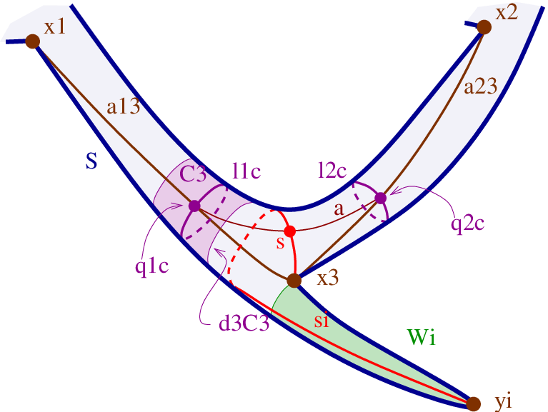
iii) $\alpha_{23}$ is a saddle arc. By Proposition 7.7(d), it suffices to prove that $d(x_{1},x_{2})\geq d(x_{1},x_{3})$ . Since $\partial_{3}C_{3}$ is equidistant from $x_{3}$ , we have $d(x_{1},x_{3})=d(x_{1},\partial_{3}C_{3})+d(\partial_{3}C_{3},x_{3})$ . Since $\partial_{3}C_{3}$ lies in the interior of $D^{\mathcal{V}}_{x_{3}}$ , we have $d(\partial_{3}C_{3},x_{3})<d(\partial_{3}C_{3},x_{2})$ . Finally, $d(x_{1},x_{2})\geq d(x_{1},\partial_{3}C_{3})+d(\partial_{3}C_{3},x_{2})$ .

Now, fix a regular $c\in\mathcal{I}_{\varepsilon}$ and let $q_{1,c}\in\alpha_{13}$ and $q_{2,c}\in\alpha_{23}$ be points at distance $c$ from $x_{3}$ . Since $\alpha_{13}$ and $\alpha_{23}$ are saddle geodesics, we have $\mathcal{V}(q_{1,c})=\mathcal{V}(q_{2,c})=c$ . Since $q_{1,c}\in C_{3}$ and $q_{2,c}\notin C_{3}$ , the points $q_{1,c},q_{2,c}$ belong to different connected components of the level set $\mathcal{V}^{-1}(c)$ . We denote such components by $\lambda_{1,c}$ and $\lambda_{2,c}$ correspondingly, and denote by $S^{\prime}$ the cylindrical subsurface of $S$ bounded by $\lambda_{1,c}$ and $\lambda_{2,c}$ . By applying Lemma 4.20, we obtain a path $\alpha$ inside $S^{\prime}$ with the following properties

•

$\alpha$ passes through a saddle point $s$ with $\mathcal{V}(s)=c^{\prime}<c$
•

$\alpha$ is contained in $\mathcal{V}^{-1}([c^{\prime},\pi))\cap S^{\prime}$
•

$\alpha$ intersects transversally the saddle geodesic $\sigma_{s}\subset S^{\prime}$ passing through $s$ .

We claim that $\sigma_{s}$ is a saddle loop based at $x_{3}$ . As a consequence, by Lemma 4.20 the loop $\sigma_{s}$ separates $q_{1,c}$ from $q_{2,c}$ on $S$ , and so it also separates $x_{1}$ and $x_{2}$ . This gives us a desired contradiction with Proposition 7.9.

In order to finally prove the above claim, note first that $\sigma_{s}$ cannot end at $x_{1}$ or at $x_{2}$ , since it is contained in $S^{\prime}$ . Suppose by contradiction that $\sigma_{s}$ has one endpoint at $y_{i}$ and let $d_{y_{i}}=d(y_{i},x_{3})$ . Lemma 4.21(a) and Lemma 4.21(d) state correspondingly that

d_{y_{i}}/2<\mathcal{V}(s)=c^{\prime}<d_{y_{i}},\;\;\;\mathcal{V}(\partial B^{\max}_{y_{i}})<d_{y_{i}}/2.

But since $\mathcal{V}(\alpha)\geq c^{\prime}>d_{y_{i}}/2$ , the second inequality implies that $\alpha\cap\partial B^{\max}_{y_{i}}=\emptyset$ . Hence $\alpha$ cannot enter $B^{\max}_{y_{i}}$ , in particular $s\notin B^{\max}_{y_{i}}$ , i.e., $d(s,y_{i})>d_{y_{i}}$ . However $\mathcal{V}(s)=d(s,y_{i})$ and so we get a contradiction with Lemma 4.21(a). Hence, $\sigma_{s}$ must be a saddle loop based at $x_{3}$ and the proof is complete. ∎

Corollary 7.15.

If $y_{i}$ is not tied to $x_{j}$ then $y_{i}$ and $x_{j}$ belong to distinct connected components of $S\setminus C_{j}$ .

Proof.

By definition $C_{1},\,C_{2},\,C_{3}$ are pairwise disjoint. And so the conclusion follows from Propositions 7.14 and 7.10(b). ∎

As a last piece of information on the cylinders $C_{j}$ , here we give an estimate of their modulus that will be needed in the proof of Theorem B(b).

Lemma 7.16.

Under the hypotheses of Theorem B(b), each Voronoi cylinder $C_{j}$ constructed above has modulus $M(C_{j})>\frac{1}{2}$ .

Proof.

Assume $j=3$ , the other cases $j=1,2$ being analogous.

Consider the Voronoi cylinder $C_{3}$ constructed in Proposition 7.10. The boundary curves of $C_{3}$ belong to the level sets $\mathcal{V}^{-1}(\pi(m+1)\varepsilon)$ and $\mathcal{V}^{-1}(\pi/4-\pi(m+1)\varepsilon)$ and the total angle of the conical points contained in the component of $S\setminus C_{3}$ that contains $x_{3}$ is at most $2\pi\left(m_{1}+\frac{1}{2}+m\varepsilon\right)<2\pi(m_{1}+1)$ . By Lemma 5.5, it follows that

M(C_{1})>\frac{1}{2\pi(m_{1}+1)}\log\left(\frac{1}{4(m+1)\varepsilon}-1\right).

As a consequence, $M(C_{1})>\frac{1}{2}$ if

\varepsilon<\frac{1}{4(m+1)\left(1+\exp\pi(\max\{m_{i}\}+1)\right)}

is satisfied. This is the case, because the right hand side is not smaller than $\frac{1}{16}\exp(-2\pi\max\{m_{i}\})$ . ∎

7.4 Disconnectedness of the moduli spaces

We can finally assemble all the information on the cylinders $C_{j}$ obtained above and prove the main result of this section.

Proof of Theorem B.

(a) Consider a spherical surface in $\text{\footnotesize{$\mathpzc{MSph}$}}_{0,m+3}(\text{\boldmath$\vartheta$})$ with conical points $x_{1},x_{2},x_{3},y_{1},\dots,y_{m}$ . By Proposition 7.7(b), each point $y_{j}$ on $S$ has a unique closest conical point among $x_{1},\,x_{2},\,x_{3}$ . Hence, to each spherical surface in $\text{\footnotesize{$\mathpzc{MSph}$}}_{0,3+m}(\text{\boldmath$\vartheta$})$ we can associate a function $\kappa:\{1,\ldots,m\}\to\{1,2,3\}$ in such a way that $x_{\kappa(i)}\in\{x_{1},x_{2},x_{3}\}$ is the point closest to $y_{i}$ . Since the $3^{m}$ functions $d(y_{i},x_{j})$ are continuous on the moduli space of metrics, by Proposition 7.7(b) the application $\mathcal{K}:\text{\footnotesize{$\mathpzc{MSph}$}}_{0,3+m}(\text{\boldmath$\vartheta$})\rightarrow\{1,2,3\}^{m}$ that sends a spherical surface to its associated vector $(\kappa(1),\ldots,\kappa(m))$ is locally constant. It follows that $\text{\footnotesize{$\mathpzc{MSph}$}}^{\kappa}_{0,3+m}(\text{\boldmath$\vartheta$}):=\mathcal{K}^{-1}(\kappa)$ is a union of connected components of $\text{\footnotesize{$\mathpzc{MSph}$}}_{0,3+m}(\text{\boldmath$\vartheta$})$ . Hence, to prove claim (a) we need to show that each $\text{\footnotesize{$\mathpzc{MSph}$}}^{\kappa}_{0,3+m}(\text{\boldmath$\vartheta$})$ is non-empty.

Consider a partition of $\{1,2,\dots,m\}$ into three disjoint subsets $I_{1},I_{2},I_{3}$ . In order to construct the metric such that $\kappa^{-1}(j)=I_{j}$ , we start first with a spherical surface of genus $0$ with three conical points $(x_{1}^{\prime},x_{2}^{\prime},x_{3}^{\prime})$ such that $\vartheta^{\prime}_{j}=m_{j}+\frac{1}{2}+\sum_{i\in I_{j}}(\varepsilon_{i}-1)$ . Such a spherical surface exists by [11] and, since the monodromy is not coaxial, we can apply Proposition 2.4 to split each point $x^{\prime}_{j}$ into a point $x_{j}$ of angle $2\pi\left(m_{j}+\frac{1}{2}\right)$ and a collection of nearby points $y_{i}$ with $i\in I_{j}$ of conical angles $2\pi\varepsilon_{i}$ . We can arrange in such a way that the function $f$ associated to such spherical surface satisfies $\kappa(I_{j})=j$ for $j=1,\,2,\,3$ simply by taking $\eta>0$ small enough in Proposition 2.4.

(b) For every $i=1,\dots,m$ consider the map $\Pi_{i}:\text{\footnotesize{$\mathpzc{M}$}}_{0,3+m}\rightarrow\text{\footnotesize{$\mathpzc{M}$}}_{0,4}$ that sends $(S,J,x_{1},x_{2},x_{3},y_{1},\dots,y_{m})$ to $(S,J,x_{1},x_{2},x_{3},y_{i})$ and let $\Pi=(\Pi_{1},\dots,\Pi_{m}):\text{\footnotesize{$\mathpzc{M}$}}_{0,3+m}\rightarrow\left(\text{\footnotesize{$\mathpzc{M}$}}_{0,4}\right)^{m}$ . Let us denote subregions $\text{\footnotesize{$\mathpzc{M}$}}_{0,4}^{(1,4)}$ , $\text{\footnotesize{$\mathpzc{M}$}}_{0,4}^{(2,4)}$ and $\text{\footnotesize{$\mathpzc{M}$}}_{0,4}^{(3,4)}$ of $\text{\footnotesize{$\mathpzc{M}$}}_{0,4}$ as in Lemma A.11. For every $\kappa\in\{1,2,3\}^{m}$ , we denote by $\text{\footnotesize{$\mathpzc{M}$}}^{\kappa}_{0,3+m}$ the subset of $\text{\footnotesize{$\mathpzc{M}$}}_{0,3+m}$ defined as

\text{\footnotesize{$\mathpzc{M}$}}^{\kappa}_{0,3+m}:=\Pi^{-1}\left(\text{\footnotesize{$\mathpzc{M}$}}_{0,4}^{(\kappa(1),4)}\times\text{\footnotesize{$\mathpzc{M}$}}_{0,4}^{(\kappa(2),4)}\times\dots\times\text{\footnotesize{$\mathpzc{M}$}}_{0,4}^{(\kappa(m),4)}\right)

and we note that such $\text{\footnotesize{$\mathpzc{M}$}}^{\kappa}_{0,3+m}$ are pairwise disjoint by Lemma A.11. In order to conclude, it is enough to show that $F_{0,3+m,\text{\boldmath$\vartheta$}}$ maps $\text{\footnotesize{$\mathpzc{MSph}$}}^{\kappa}_{0,3+m}(\text{\boldmath$\vartheta$})$ to $\text{\footnotesize{$\mathpzc{M}$}}^{\kappa}_{0,3+m}$ .

We recall that on each such surface $S$ there exists a cylinder $C_{\kappa(i)}$ (Proposition 7.10) of modulus greater than $\frac{1}{2}$ (Lemma 7.16) such that the pairs of conical points $\{x_{\kappa(i)},\,y_{i}\}$ and $\{x_{1},x_{2},x_{3}\}\setminus\{x_{\kappa(i)}\}$ are contained in different components of $S\setminus C_{\kappa(i)}$ (Proposition 7.14). This in particular implies that a simple closed curve $\gamma_{j}$ homotopic to $C_{j}$ has $\mathrm{Ext}_{\gamma_{j}}(\dot{S},J)<2$ and so $\mathrm{Ext}_{\gamma_{j}}(S\setminus\{x_{1},x_{2},x_{3},y_{i}\},J)<2$ . It follows from Lemma A.11 that $(\Pi_{i}\circ F_{0,3+m,\text{\boldmath$\vartheta$}})(\text{\footnotesize{$\mathpzc{MSph}$}}^{\kappa}_{0,3+m}(\text{\boldmath$\vartheta$}))$ is contained inside $\text{\footnotesize{$\mathpzc{M}$}}_{0,4}^{(\kappa(i),4)}$ and so

F_{0,3+m,\text{\boldmath$\vartheta$}}(\text{\footnotesize{$\mathpzc{MSph}$}}^{\kappa}_{0,3+m}(\text{\boldmath$\vartheta$}))\subseteq\text{\footnotesize{$\mathpzc{M}$}}^{\kappa}_{0,3+m}

as desired. ∎

8 Disks with one conical point

The purpose of this section is to estimate the area of a topological disk endowed with a spherical metric with at most one conical point and a short boundary. Such computation will be needed to calculate the area of almost bubbling surfaces in Section 9. For this reason, we will use the symbol $\mathpzc{B}$ to denote such topological disks.

In order to measure how short the boundary of $\mathpzc{B}$ is, we introduce the following quantity.

Definition 8.1 ( $\lambda$ -invariant).

Let $\mathpzc{B}^{0}$ be a spherical disk without conical points and $\mathpzc{B}^{1}$ be a spherical with one conical point $x$ . We define their $\lambda$ -invariant as

\lambda_{0}(\mathpzc{B}^{0}):=\left(\frac{\ell(\partial\mathpzc{B}^{0})}{2\pi}\right)^{2}\qquad\text{and}\qquad\lambda_{1}(\mathpzc{B}^{1}):=\frac{\ell(\partial\mathpzc{B}^{1})}{d(x,\partial\mathpzc{B}^{1})}.

The following result is an essential ingredient of our proof of the systole inequality.

Theorem 8.2 (Disks with one conical point and short boundary).

Let $\mathpzc{B}^{1}$ be a spherical disk with one conical point $x$ of angle $2\pi\vartheta$ and assume that $\lambda_{1}(\mathpzc{B}^{1})<\frac{1}{2}$ . Then there exists $b^{1}\in\mathbb{Z}_{\geq 0}$ such that

\frac{1}{2\pi}\Big|\mathrm{Area}(\mathpzc{B}^{1})-4\pi(\vartheta+b^{1})\Big|<\frac{\ell(\partial\mathpzc{B}^{1})}{d(x,\partial\mathpzc{B}^{1})}=\lambda_{1}(\mathpzc{B}^{1}).

Remark 8.3.

The hypothesis $\lambda_{1}(\mathpzc{B}^{1})<\frac{1}{2}$ is only used at the very end of proof of Theorem 8.2. The analogous estimate for disks without conical points is proven in Corollary 8.12.

The proof of Theorem 8.2 proceeds as follows. First we reduce the calculation of the area of the disk $\mathpzc{B}^{1}$ to that of a disk $D_{\alpha}$ without conical points, which is obtained by cutting $\mathpzc{B}^{1}$ along a geodesic arc $\alpha$ that joins $x$ to $\partial\mathpzc{B}^{1}$ . Then we compute the area of $D_{\alpha}$ using the degree function of a developing map $\iota:D_{\alpha}\rightarrow\mathbb{S}^{2}$ and the algebraic area of its boundary $\iota(\partial D_{\alpha})$ relative to a base point $Z\in\mathbb{S}^{2}$ . Such algebraic area is an invariant of oriented loops in $\mathbb{S}^{2}$ which has good additive properties and is tightly related to the degree function of $\iota$ . The final estimate for the algebraic area of $\iota(\partial D_{\alpha})$ relies on an area estimate for isosceles spherical triangles embedded in $\mathbb{S}^{2}$ and on the isoperimetric inequality for domains in $\mathbb{S}^{2}$ .

8.1 Degree functions and algebraic area on $\mathbb{S}^{2}$

In this subsection we introduce the degree function and the algebraic area associated to an oriented loop in $\mathbb{S}^{2}$ and we prove some elementary relation between such quantities, the classical degree and the standard area.

Definition 8.4 (Degree function of an oriented loop in $\mathbb{S}^{2}$ relative to a base point).

Let $\xi$ be a piecewise smooth oriented closed curve on $\mathbb{S}^{2}$ . Let $Z$ be a point in the complement $\mathbb{S}^{2}\setminus\xi$ . The degree function $\deg_{Z}(\xi):\mathbb{S}^{2}\setminus\xi\rightarrow\mathbb{Z}$ is defined as

\deg_{Z}(\xi)(Y):=[YZ]\cdot\xi

for every point $Y\in\mathbb{S}^{2}\setminus\xi$ , where $[YZ]$ is (the relative homology class of) any smooth path that runs from $Y$ to $Z$ and $[YZ]\cdot\xi$ is the intersection number (with sign) of two curves.

Definition 8.5 (Algebraic area of an oriented loop in $\mathbb{S}^{2}$ ).

The algebraic area of $\xi$ with respect to $Z$ is defined as

\mathrm{Alg}_{Z}(\xi)=\int_{\mathbb{S}^{2}}\deg_{Z}(\xi)\cdot\,\omega

where $\omega$ is the standard area form on $\mathbb{S}^{2}$ .

Note that the algebraic area $\mathrm{Alg}_{Z}(\xi)$ is continuous for piecewise-smooth deformations of $\xi$ in $\mathbb{S}^{2}\setminus Z$ . The following standard lemma justifies the name of degree function.

Lemma 8.6 (Degree of a map from a disk to $\mathbb{S}^{2}$ and degree of its boundary).

Let $D$ be an oriented disk and $\varphi:D\to\mathbb{S}^{2}$ be a piecewise smooth map and let $\xi=\partial\varphi:\partial D\rightarrow\mathbb{S}^{2}$ be the restriction of $\varphi$ to the boundary $\partial D$ , which is endowed with the induced orientation. Choose a regular point $Z\in\mathbb{S}^{2}\setminus\xi$ for $\varphi$ . Then the degree function $\deg(\varphi):\mathbb{S}^{2}\setminus\xi\rightarrow\mathbb{Z}$ of the map $\varphi$ coincides with $\deg(\varphi)(Z)+\deg_{Z}(\xi)$ .

We omit the proof since it is clear. The next two lemmas are straightforward as well.

Lemma 8.7 (Additivity of the degree function).

Let $P,Q$ be two points on $\mathbb{S}^{2}$ and $\xi_{1}$ , $\xi_{2}$ , $\xi_{3}$ piecewise smooth paths that run from $P$ to $Q$ . Choose $Z\in\mathbb{S}^{2}\setminus(\xi_{1}\cup\xi_{2}\cup\xi_{3})$ and let $\xi_{ij}$ be the oriented loop based at $P$ obtained by travelling first along $\xi_{j}$ and then along $\xi_{i}^{-1}$ . Then for any $Y\in\mathbb{S}^{2}\setminus(\xi_{1}\cup\xi_{2}\cup\xi_{3})$ we have

\deg_{Z}(\xi_{13})(Y)=\deg_{Z}(\xi_{12})(Y)+\deg_{Z}(\xi_{23})(Y).

Lemma 8.8 (Area of a spherical disk and algebraic area of its boundary).

Let $D$ be a disk with a spherical metric and piecewise smooth boundary. Let $\iota:D\to\mathbb{S}^{2}$ be an orientation preserving developing map and let $Z\in\mathbb{S}^{2}\setminus\iota(\partial D)$ . Then the following equality holds

\mathrm{Area}(D)=4\pi\deg(\iota)(Z)+\mathrm{Alg}_{Z}(\iota(\partial D)).

Proof.

Since $\iota$ is locally isometric we clearly have $\mathrm{Area}(D)=\int_{D}\iota^{*}(\omega)$ . Now the statement follows from Lemma 8.6, since $\int_{D}\iota^{*}(\omega)=\int_{\mathbb{S}^{2}}\deg(\iota)\omega$ . ∎

8.2 Algebraic area of short curves

In this subsection we estimate the algebraic area of curves on $\mathbb{S}^{2}$ of length less than $2\pi$ . Such estimate takes the form of an isoperimetric inequality.

Lemma 8.9 (Isoperimetric inequality in $\mathbb{S}^{2}$ for the algebraic area).

Let $\xi\subset\mathbb{S}^{2}$ be an oriented piecewise smooth curve with $\ell(\xi)<2\pi$ . Let $Z$ be a point on $\mathbb{S}^{2}$ separated from $\xi$ by a geodesic circle in $\mathbb{S}^{2}$ . Then $|\mathrm{Alg}_{Z}(\xi)|<\ell(\xi)^{2}/2\pi$ .

The above lemma is probably well-known but for the sake of completeness we will provide a proof that relies on the following classical isoperimetric inequality (see [16, Lemma 6.1]).

Lemma 8.10 (Isoperimetric inequality for disk domains in $\mathbb{S}^{2}$ ).

Let $\Omega\subset\mathbb{S}^{2}$ be a disk with piecewise smooth boundary. Then $\ell(\partial\Omega)^{2}\geq\mathrm{Area}(\Omega)\left(4\pi-\mathrm{Area}(\Omega)\right)$ . In particular, if $\mathrm{Area}(\Omega)<2\pi$ , then $\ell(\partial\Omega)^{2}>2\pi\cdot\mathrm{Area}(\Omega)$ .

Before proving Lemma 8.9, we recall that the concatenation at times $(t_{1},t_{2})$ of two loops $\xi_{1},\xi_{2}:S^{1}\rightarrow\mathbb{S}^{2}$ that satisfy $\xi_{1}(t_{1})=\xi_{2}(t_{2})$ is the loop $(\xi_{1})\,_{t_{1}}\!\!\ast_{t_{2}}\!(\xi_{2}):S^{1}\rightarrow\mathbb{S}^{2}$ defined as

(\xi_{1})\,_{t_{1}}\!\!\ast_{t_{2}}\!(\xi_{2})(t)=\begin{cases}\xi_{1}(t_{1}+2t)&\text{if $t\in[0,\frac{1}{2}]$}\\ \xi_{2}(t_{2}+2t-1)&\text{if $t\in[\frac{1}{2},1]$}\end{cases}

where we have identified $S^{1}$ with $\mathbb{R}/\mathbb{Z}$ . It is clearly possible to concatenate more than two loops (at different times) iterating the above procedure.

Lemma 8.11 (Loops generically immersed in $\mathbb{S}^{2}$ are concatenations of simple loops).

Let $\xi:S^{1}\rightarrow\mathbb{S}^{2}$ be a piecewise smooth curve with a finite number of self-intersections. Then, up to a reparametrization, $\xi$ is a concatenation of finitely many simple loops $\xi_{1},\dots,\xi_{k}$ such that $\xi_{i}$ and $\xi_{j}$ intersect at finitely many points for every $i\neq j$ .

Proof.

By assumption, the set of non-injectivity points $N=\{t\in S^{1}\,|\,\exists t^{\prime}\neq t\ \text{such that $\xi(t^{\prime})=\xi(t)$}\}$ is finite. We proceed by induction on $|N|$ .

For $|N|=0$ , the loop $\xi$ is already simple. Assume then $N\neq\emptyset$ and consider $u=\min\{d_{S^{1}}(t^{\prime},t)\,|\,\xi(t^{\prime})=\xi(t)\ \text{with $t^{\prime}\neq t$}\}>0$ . Let $(t_{1},t_{1}+u)$ be a couple such that $\xi(t_{1})=\xi(t_{1}+u)$ . Then $\xi$ is the reparametrized concatenation $(\xi_{1})\ast(\xi^{\prime}_{1})$ , where $\xi_{1}$ is a reparametrization of $\xi|_{[t_{1},t_{1}+u]}$ and $\xi^{\prime}_{1}$ is a reparametrization of the remaining portion of $\xi$ . By the minimality of $u$ , the loop $\xi_{1}$ is simple. Moreover, the set $N^{\prime}$ of non-injectivity points of $\xi^{\prime}_{1}$ satisfies $|N^{\prime}|<|N|$ and so the curve $\xi^{\prime}_{1}$ is a reparametrized concatenation of finitely many simple loops $\xi_{2},\dots,\xi_{k}$ by induction. It follows that $\xi$ is a reparametrized concatenation of $\xi_{1},\dots,\xi_{k}$ . Finally, for $i\neq j$ the simple loops $\xi_{i}$ and $\xi_{j}$ can only intersect at $\xi(N)$ , which is a finite subset of $\mathbb{S}^{2}$ . ∎

Proof of Lemma 8.9.

Note first that, since $\ell(\xi)<2\pi$ , a geodesic circle $E$ on $\mathbb{S}^{2}$ that does not intersect $\xi$ indeed exists, and so we can choose $Z$ in the component of $\mathbb{S}^{2}\setminus E$ that does not contain $\xi$ .

After perturbing $\xi$ , if necessary, we may assume that $\xi$ has finite number of self-intersections in $\mathbb{S}^{2}$ . Denote by $\Omega_{0}$ the connected component of $\mathbb{S}^{2}\setminus\xi$ that contains $Z$ .

Let us now give a different presentation of the function $\deg_{Z}(\xi)$ . Thanks to Lemma 8.11, the curve $\xi$ can be decomposed into a finite number of simple loops $\xi_{1},\ldots,\xi_{k}$ . Each loop $\xi_{i}$ encloses a disk $\Omega_{i}$ , whose interior is disjoint from $\Omega_{0}$ . We underline that two disks $\Omega_{i}$ and $\Omega_{j}$ may well overlap if $i,j\neq 0$ .

It follows from Lemma 8.7 that

\deg_{Z}(\xi)=\sum_{i}\deg_{Z}(\xi_{i}).

Since the curves $\xi_{i}$ are separated from $Z$ by the geodesic circle $E$ , we deduce

\mathrm{Alg}_{Z}(\xi)=\int_{\mathbb{S}^{2}}\deg_{Z}(\xi)\omega=\int_{\mathbb{S}^{2}}\sum_{i}\deg_{Z}(\xi_{i})\omega=\sum_{i}\pm\mathrm{Area}(\Omega_{i}).

Using Lemma 8.10 we conclude that

|\mathrm{Alg}_{Z}(\xi)|\leq\sum_{i}\mathrm{Area}(\Omega_{i})<\sum_{i}\ell(\xi_{i})^{2}/2\pi\leq\ell(\xi)^{2}/2\pi

because $\sum_{i}\ell(\xi_{i})=\ell(\xi)$ . ∎

As a consequence of Lemma 8.9, we obtain the following isoperimetric inequality for the area of an abstract spherical disk $\mathpzc{B}^{0}$ with no conical points, which will be needed in the proof of the systole inequality.

Corollary 8.12 (Isoperimetric inequality for spherical disks with short boundary).

Let $\mathpzc{B}^{0}$ be a disk with spherical metric and no conical points such that $\partial\mathpzc{B}^{0}$ is piecewise smooth and $\ell(\partial\mathpzc{B}^{0})<2\pi$ . Then

\frac{1}{2\pi}\Big|\mathrm{Area}(\mathpzc{B}^{0})-4\pi b^{0}\Big|<\left(\frac{\ell(\partial\mathpzc{B}^{0})}{2\pi}\right)^{2}=\lambda_{0}(\mathpzc{B}^{0})

for some $b^{0}\in\mathbb{Z}_{\geq 0}$ .

Proof.

Consider a developing map $\iota:\mathpzc{B}^{0}\to\mathbb{S}^{2}$ . Since $\ell(\partial\mathpzc{B}^{0})<2\pi$ , there is a geodesic circle $E\subset\mathbb{S}^{2}$ disjoint from $\iota(\partial\mathpzc{B}^{0})$ . Let $O$ be the center of the component of $\mathbb{S}^{2}\setminus E$ which does not contain $\iota(\partial\mathpzc{B}^{0})$ . By Lemma 8.8 we have $\mathrm{Area}(\mathpzc{B}^{0})=4\pi\deg(\iota)(O)+\mathrm{Alg}_{O}(\iota(\partial\mathpzc{B}^{0}))$ . Now the statement follows from Lemma 8.9, because $\iota$ is orientation-preserving and so $b^{0}:=\deg(\iota)(O)\geq 0$ . ∎

8.3 Isosceles spherical triangles

In this section we estimate the area of certain isosceles triangles embedded in $\mathbb{S}^{2}$ with one short side.

The following lemma will be needed in the proof of Theorem 8.2.

Lemma 8.13 (Area estimate for isosceles triangles).

Let $T\subset\mathbb{S}^{2}$ be a solid triangle with geodesic sides and endow its boundary $\partial T$ with the induced orientation and then its vertices $P,O,Q$ with the cyclic orientation $P\prec O\prec Q$ . Suppose that $|OP|=|OQ|=r$ and that $|PQ|<r\cdot\lambda_{1}$ for some $\lambda_{1}\in(0,1)$ . Then

|\mathrm{Alg}_{Z}(\partial T)-4\pi\theta|=|\mathrm{Area}(T)-4\pi\theta|<\pi\lambda_{1}

for any point $Z\in\mathbb{S}^{2}\setminus T$ , where $2\pi\theta=\widehat{O}$ is the internal angle of $T$ at $O$ .

Proof.

The equality holds since $\mathrm{Alg}_{Z}(\partial T)=\mathrm{Area}(T)$ thanks to the choice of the cyclic orientation of the vertices of $T$ and because $Z\notin T$ . So we only need to prove the inequality on the right.

Suppose first $r\in\left[\frac{\pi}{2},\pi\right)$ . Let $O^{\prime}$ be the point on $\mathbb{S}^{2}$ opposite to $O$ and let $T^{\prime}\subset\mathbb{S}^{2}\setminus\accentset{\circ}{T}$ be the solid triangle with edges consisting of the shortest geodesics $O^{\prime}P$ and $O^{\prime}Q$ and of the edge $PQ$ of $T$ . Since $T\cup T^{\prime}$ is a bigon with angles $2\pi\theta$ ,

\mathrm{Area}(T)+\mathrm{Area}(T^{\prime})=4\pi\theta.

Moreover, $|O^{\prime}P|=|O^{\prime}Q|\leq\frac{\pi}{2}$ and so the triangle $T^{\prime}$ can be embedded inside an isosceles triangle with sides of lengths $\frac{\pi}{2},\,\,\frac{\pi}{2}\,|PQ|$ . Hence the area of $T^{\prime}$ is bounded by the length of the side $PQ$ . As a consequence, $|\mathrm{Area}(T)-4\pi\theta|\leq|PQ|<r\cdot\lambda_{1}\leq\pi\lambda_{1}$ because $|PQ|<r\cdot\lambda_{1}$ by assumption.

Suppose now $r\in\left(0,\frac{\pi}{2}\right)$ . Assume first $\theta\leq\frac{1}{2}$ . Applying Lemma 8.14 to triangle $T$ , we get $\theta<\frac{\lambda_{1}}{4}$ . Since $\mathrm{Area}(T)<4\pi\theta$ , we conclude that

|\mathrm{Area}(T)-4\pi\theta|<4\pi\theta<\pi\lambda_{1}.

Finally, consider the case $\theta\geq\frac{1}{2}$ and let $T^{\prime}=\mathbb{S}^{2}\setminus\accentset{\circ}{T}$ be the complementary of $T$ inside $\mathbb{S}^{2}$ , so that $\mathrm{Area}(T)+\mathrm{Area}(T^{\prime})=4\pi$ . Since $T^{\prime}$ has internal angle $2\pi(1-\theta)$ at $O$ , we have just seen that $(1-\theta)<\frac{\lambda_{1}}{4}$ and so $4\pi(1-\theta)<\pi\lambda_{1}$ . From $\mathrm{Area}(T^{\prime})<4\pi(1-\theta)$ we deduce that $\mathrm{Area}(T)\in\left(4\pi\theta,4\pi\right)$ and so we conclude that $|\mathrm{Area}(T)-4\pi\theta|<\pi\lambda_{1}$ . ∎

The above proof relies on the following computation in the case $r\in\left(0,\frac{\pi}{2}\right)$ and $\theta\leq\frac{1}{2}$ .

Lemma 8.14.

Fix $\theta\in\left(0,\frac{1}{2}\right)$ , $r\in\left(0,\frac{\pi}{2}\right)$ , and $\lambda_{1}\in(0,1)$ . Let $POQ$ be a convex spherical triangle with angle $2\pi\theta$ at $O$ , and with $|OP|=|OQ|=r$ and $|QP|=\lambda_{1}r$ . Then $\theta<\lambda_{1}/4$ .

Proof.

Let $R$ be the midpoint of $QP$ and consider the triangle $POR$ , which has angle $\pi\theta$ at $O$ and $\frac{\pi}{2}$ at $R$ and such that $|RP|=r\lambda_{1}/2$ .

Applying the sine rule to the sides $PO$ and $OR$ of triangle $POR$ , we get

\sin(\pi\theta)=\frac{\sin(r\lambda_{1}/2)}{\sin(r)}=\varphi(r).

Note that for $r=\frac{\pi}{2}$ we get $\theta=\lambda_{1}/4$ . Hence, to prove the lemma, it is enough to show that $\varphi$ is strictly increasing on $(0,\frac{\pi}{2})$ , namely that for $r\in(0,\frac{\pi}{2})$ we have $\varphi^{\prime}(r)>0$ . The latter is equivalent to proving

(\lambda_{1}/2)\cos(r\lambda_{1}/2)\sin(r)-\cos(r)\sin(r\lambda_{1}/2)>0.

This inequality holds since $t\tan(r)>\tan(t\eta)$ for all $t\in(0,1)$ and $r\in(0,\pi/2)$ . ∎

8.4 Area estimate of a disk with one conical point and short boundary

We can finally assemble all the ingredients to prove our wished estimate for the area a disk with one conical point and short boundary.

Proof of Theorem 8.2.

Let us write $\vartheta=\lfloor{\vartheta}\rfloor+\theta$ , where $\theta=\{\vartheta\}\in[0,1)$ . Let $\alpha\subset\mathpzc{B}^{1}$ be a geodesic of length $r=d(x,\partial\mathpzc{B}^{1})$ that joins $x$ with a point $y$ on $\partial\mathpzc{B}^{1}$ . Denote by $D_{\alpha}$ the disk obtained from $\mathpzc{B}^{1}$ by cutting it along $\alpha$ and completing. Denote by $x_{O}$ the point in $D_{\alpha}$ corresponding to $x$ and by $y_{P}$ and $y_{Q}$ two points corresponding to $y$ . The points $x_{O}$ , $y_{P}$ , $y_{Q}$ cut $\partial D_{\alpha}$ into two geodesic segments $y_{P}x_{O}$ , $x_{O}y_{Q}$ and a non-geodesic path $y_{Q}y_{P}$ . We choose the orientation on $D_{\alpha}$ so that points $y_{P}\prec x_{O}\prec y_{Q}$ according to the induced orientation on $\partial D_{\alpha}$ .

Let now $\iota:D_{\alpha}\to\mathbb{S}^{2}$ be an orientation preserving developing map. Call $O=\iota(x_{O})$ , $P=\iota(y_{P})$ and $Q=\iota(y_{Q})$ and denote by $PO$ the geodesic arc $\iota(y_{P}x_{O})$ and by $OQ$ the geodesic arc $\iota(x_{O}y_{Q})$ . To define $PQ$ note that $d(P,Q)\leq\ell(\partial\mathpzc{B}^{1})=\lambda_{1}(\mathpzc{B}^{1})r<r<\pi$ and so we can choose $PQ$ to be the unique geodesic segment between $P$ and $Q$ of length less than $\pi$ . Finally, let $T$ be a solid triangle in $\mathbb{S}^{2}$ with vertices $P,O,Q$ and sides $PO$ , $OQ$ , and $PQ$ , and with angle $2\pi\theta$ at $O$ (such a $T$ is unique, unless $\theta=\frac{1}{2}$ ).

Pick a point $Z$ in $\mathbb{S}^{2}\setminus T$ at distance $\lambda_{1}(\mathpzc{B}^{1})$ from $O$ . Since the conical angle at $x$ is equal to $2\pi\left(\lfloor{\vartheta}\rfloor+\theta\right)$ , it is easy to see now that $\deg_{Z}(\iota)=\lfloor{\vartheta}\rfloor+b^{1}$ for some $b^{1}\geq 0$ . We deduce from Lemma 8.8, that

\mathrm{Area}(\mathpzc{B}^{1})=\mathrm{Area}(D_{\alpha})=\mathrm{Alg}_{Z}(\iota(\partial D_{\alpha}))+4\pi(\lfloor{\vartheta}\rfloor+b^{1}).

Hence, we need to show $|\mathrm{Alg}_{Z}(\iota(\partial D_{\alpha}))-4\pi\theta|\leq 2\pi\lambda_{1}(\mathpzc{B}^{1})$ .

In order to prove this inequality let us present $\iota(\partial D_{\alpha})$ as a sum of two curves. The first is the boundary of triangle $T$ and the second is a curve $\xi$ , composed of segment $PQ$ and the curvy part of $\iota(\partial D_{\alpha})$ going from $Q$ to $P$ . Clearly $\ell(\xi)\leq 2\ell(\partial\mathpzc{B}^{1})$ and so, by our hypotheses, $\ell(\xi)\leq 2r\lambda_{1}(\mathpzc{B}^{1})$ . Applying the additivity property of Lemma 8.7 and the inequalities of Lemma 8.9 and Lemma 8.13 we obtain

	$\displaystyle\|\mathrm{Alg}_{Z}(\iota(\partial D_{\alpha}))-4\pi\theta\|$	$\displaystyle=\|\mathrm{Alg}_{Z}(T)-4\pi\theta+\mathrm{Alg}_{Z}(\xi)\|\leq$
		$\displaystyle\leq\|\mathrm{Alg}_{Z}(T)-4\pi\theta\|+\|\mathrm{Alg}_{Z}(\xi)\|\leq\pi\lambda_{1}(\mathpzc{B}^{1})+\left(2r\lambda_{1}(\mathpzc{B}^{1})\right)^{2}/2\pi<2\pi\lambda_{1}(\mathpzc{B}^{1})$

because $\lambda_{1}(\mathpzc{B}^{1})<\frac{1}{2}$ implies $2r\lambda_{1}(\mathpzc{B}^{1})<\pi$ . ∎

9 Almost bubbling surfaces and systole inequality

In this section we will prove Theorem C which relates the extremal systole, that measures how much the surface is conformally far from degenerating, and the spherical systole, that measures how much the surface is metrically far from degenerating. As mentioned in the introduction, if the extremal systole is small, then the spherical systole is small. In the following theorem we show that the converse also holds, whenever $\mathrm{NB}_{\text{\boldmath$\vartheta$}}>0$ .

Theorem C (Systole inequality).

(i)

$\mathrm{Ext}\mathrm{sys}(\dot{S})\geq\frac{2\pi\|\text{\boldmath$\vartheta$}\|_{1}}{\log(1/\varepsilon)}$ .
(ii)

$\mathrm{NB}_{\text{\boldmath$\vartheta$}}(S)\geq\varepsilon$ .

Then the following inequality holds:

\mathrm{sys}(S,\text{\boldmath$x$})\geq\left(\frac{\varepsilon}{4\pi\|\text{\boldmath$\vartheta$}\|_{1}}\right)^{-3\chi(\dot{S})+1}.

(

\clubsuit

)

In Appendix A.2 we will show through a sequence of examples that the estimate for the extremal systole determined by Theorem C is reasonably sharp.

9.1 Non-bubbling parameter

We recall from Section 1.3.3 that the value $\frac{1}{2\pi}\mathrm{Area}(S)\in\mathbb{R}_{\geq 0}$ of an $\varepsilon$ -bubbling spherical surface $S$ with conical points of angles $2\pi\text{\boldmath$\vartheta$}$ sits at distance at most $\varepsilon$ from the subset

\mathrm{ACrit}_{\text{\boldmath$\vartheta$}}(S)=\left\{2b+2\|\text{\boldmath$\vartheta$}_{I}\|\ \big|\ I\subseteq\{1,\dots,n\},\ b\in\mathbb{Z}_{\geq 0}\right\}.

Thus, an obstruction $\varepsilon$ -bubbling is exactly given by $\mathrm{NB}_{\text{\boldmath$\vartheta$}}(S)\geq\varepsilon$ . Here we collect a few basic properties of such quantity.

Lemma 9.1 (Elementary properties of the non-bubbling parameter).

The subsets $\mathrm{Crit}_{\text{\boldmath$\vartheta$}}(S)$ and $\mathrm{ACrit}_{\text{\boldmath$\vartheta$}}(S)$ satisfy $\mathrm{ACrit}_{\text{\boldmath$\vartheta$}}(S)=\mathrm{Crit}_{\text{\boldmath$\vartheta$}}(S)+\|\text{\boldmath$\vartheta$}\|_{1}$ and so $\mathrm{NB}_{\text{\boldmath$\vartheta$}}(S)=d_{\mathbb{R}}(\chi(S,\text{\boldmath$\vartheta$}),\,\mathrm{ACrit}_{\text{\boldmath$\vartheta$}}(S))$ . Moreover, the following holds.

(a)

If $\chi(S,\text{\boldmath$\vartheta$})\geq 0$ , then $\mathrm{NB}_{\text{\boldmath$\vartheta$}}(S)\leq 1$ . In particular, this holds whenever there exists a spherical metric on $S$ with conical singularities at $x$ of angles $2\pi\text{\boldmath$\vartheta$}$ .
(b)

If $\chi(S,\text{\boldmath$\vartheta$})\leq 0$ , then $\mathrm{NB}_{\text{\boldmath$\vartheta$}}(S)=-\chi(S,\text{\boldmath$\vartheta$})$ since $0\in\mathrm{ACrit}_{\text{\boldmath$\vartheta$}}(S)$ .

Proof.

The first claim is obvious. As for (a), note that $\mathrm{ACrit}_{\text{\boldmath$\vartheta$}}\supseteq 2\mathbb{Z}_{\geq 0}$ and so

\mathrm{NB}_{\text{\boldmath$\vartheta$}}(S)=d_{\mathbb{R}}(\chi(S,\text{\boldmath$\vartheta$}),\,\mathrm{ACrit}_{\text{\boldmath$\vartheta$}}(S))\leq d_{\mathbb{R}}(\chi(S,\text{\boldmath$\vartheta$}),\,2\mathbb{Z}_{\geq 0})\leq 1

Property (b) is immediate, since $\mathrm{ACrit}_{\text{\boldmath$\vartheta$}}$ contains only non-negative values and $0\in\mathrm{ACrit}_{\text{\boldmath$\vartheta$}}$ . ∎

Remark 9.2 (Upper bound for $\mathcal{V}$ in terms of $\mathrm{NB}_{\text{\boldmath$\vartheta$}}(S)$ ).

If $S$ is endowed with a spherical metric with singularities of angles $2\pi\text{\boldmath$\vartheta$}$ , then

\frac{1}{2\pi}\mathrm{Area}(S)=\chi(S,\text{\boldmath$\vartheta$})=d_{\mathbb{R}}\left(\chi(S,\text{\boldmath$\vartheta$}),\,0\right)\geq\mathrm{NB}_{\text{\boldmath$\vartheta$}}(S).

As a consequence,

\max(\mathcal{V})\geq\sqrt{2\mathrm{NB}_{\text{\boldmath$\vartheta$}}(S)\|\text{\boldmath$\vartheta$}\|_{1}^{-1}}

by applying Lemma 5.7 and the previous inequality.

As mentioned in the introduction, another important property of the non-bubbling parameter is that its positivity prevents spherical metrics from having coaxial monodromy.

Lemma 9.3 (Coaxial metrics have vanishing non-bubbling parameter).

Let $(S,\text{\boldmath$x$},h)$ be a spherical surface with conical points of angles $2\pi\cdot\text{\boldmath$\vartheta$}$ . If $(S,\text{\boldmath$x$})$ has coaxial monodromy, then $\mathrm{NB}_{\text{\boldmath$\vartheta$}}(S,\text{\boldmath$x$})=0$ .

Proof.

Fix a universal cover $\tilde{\dot{S}}$ of $\dot{S}$ , a developing map $\iota:\tilde{\dot{S}}\rightarrow\mathbb{S}^{2}$ to the standard sphere $(\mathbb{S}^{2},h_{\mathbb{S}^{2}})$ and a compatible monodromy representation $\rho:\pi_{1}(\dot{S})\rightarrow\mathrm{SO}_{3}(\mathbb{R})$ . Since $\rho$ is coaxial by hypothesis, there exist antipodal points $O,O^{\prime}$ in $\mathbb{S}^{2}$ that are fixed by the image of $\rho$ . Let $G\subset\mathrm{PSL}_{2}(\mathbb{C})$ be the real 1-parameter subgroup of Möbius transformations of $\mathbb{S}^{2}\cong\mathbb{C}\mathbb{P}^{1}$ that fix $O,O^{\prime}$ and send every meridian between the two poles $O,O^{\prime}$ to itself. Clearly, every element $g\in G$ commutes with the image of $\rho$ and so the metric $\iota^{*}g^{*}h_{\mathbb{S}^{2}}$ descends to a spherical metric $h_{g}$ on $(S,\text{\boldmath$x$})$ , which is conformally equivalent to $h$ .

Let $\sigma\subset S$ be a geodesic arc that realizes the systole and let $\tilde{\sigma}\subset\tilde{\dot{S}}$ be a lift of its. Since $\sigma$ has length at most $\frac{\pi}{2}$ by Lemma 3.10, the closure of $\iota(\tilde{\sigma})$ inside $\mathbb{S}^{2}$ cannot contain both $O$ and $O^{\prime}$ .

Hence, for every $s>0$ there exists $g\in G$ such that the $h_{g}$ -length of $\sigma$ is at most $s$ and so $(S,\text{\boldmath$x$},h_{g})$ has systole at most $s$ . Since $s>0$ is arbitrary, it follows from Theorem C that $\mathrm{NB}_{\text{\boldmath$\vartheta$}}(S,\text{\boldmath$x$})=0$ . ∎

We underline that the above Lemma 9.3 can be proven in a different way, and in particular without invoking Theorem C. Indeed, one could show that, by using suitable elements $g\in G$ , one can produce metrics $h_{g}$ whose mass concentrates near certain points $x_{i}$ with $i\in I$ and near other $b\geq 0$ smooth points, so that the value of the area of $h_{g}$ (and so of $h$ ) can be estimated to be arbitrarily close to $2\pi\cdot(2b+2\|\text{\boldmath$\vartheta$}_{I}\|_{1})$ .

9.2 Almost bubbling surfaces

In this section we give a precise definition of $\varepsilon$ -bubbling spherical surface mentioned in the introduction and we show that such surfaces have small non-bubbling parameter. The definition relies on the $\lambda$ -invariant of a spherical disk with at most one conical point, introduced in Section 8.

Definition 9.4 ( $\varepsilon$ -bubbling surfaces).

Let $\varepsilon\in(0,\frac{1}{2})$ . An $\varepsilon$ -bubbling decomposition of a spherical surface $S$ with conical points $x$ is the datum of a subset $I\subseteq\{1,2,\dots,n\}$ and a partition of $S$ as a union of

•

finitely many disks $\mathpzc{B}^{0}_{j}$ without conical points,
•

a disk $\mathpzc{B}^{1}_{i}$ with one conical point $x_{i}$ for each $i\in I$ , and
•

a subsurface $S^{c}$ (called core),

such that

\frac{1}{2\pi}\mathrm{Area}(S^{c})+\sum_{j}\lambda_{0}(\mathpzc{B}^{0}_{j})+\sum_{i\in I}\lambda_{1}(\mathpzc{B}^{1}_{i})<\varepsilon.

We say that $(S,\text{\boldmath$x$})$ is $\varepsilon$ -bubbling if it admits an $\varepsilon$ -bubbling decomposition and that it is almost bubbling if it is $\varepsilon$ -bubbling for some $\varepsilon$ .

The following statement is a simple application of Theorem 8.2 and Corollary 8.12.

Theorem 9.5 (Almost bubbling implies small non-bubbling parameter).

Let $S$ be a spherical surface with conical points $x$ of angles $2\pi\text{\boldmath$\vartheta$}$ . If $S$ is $\varepsilon$ -bubbling, then $\mathrm{NB}_{\text{\boldmath$\vartheta$}}(S,\text{\boldmath$x$})<\varepsilon$ .

Proof.

Consider an $\varepsilon$ -bubbling decomposition of $S$ . An example for $(g,n)=(1,7)$ with $I=\{2,4\}$ and one $\mathpzc{B}^{0}_{1}$ is illustrated in Figure 9.4.

Applying Corollary 8.12 to each $\mathpzc{B}^{0}_{j}$ and Theorem 8.2 to each $\mathpzc{B}^{1}_{i}$ , we get

\frac{1}{2\pi}\left|\mathrm{Area}(\mathpzc{B}^{0}_{j})-4\pi b^{0}_{j}\right|<\lambda_{0}(\mathpzc{B}^{0}_{j}),\quad\frac{1}{2\pi}\left|\mathrm{Area}(\mathpzc{B}^{1}_{i})-4\pi(b^{1}_{i}+\vartheta_{i})\right|<\lambda_{1}(\mathpzc{B}^{1}_{i})

(4)

for suitable integers $b^{0}_{j},\,b^{1}_{i}\geq 0$ . As a consequence, setting $b=\sum_{j}b^{0}_{j}+\sum_{i\in I}b^{1}_{i}$ , we obtain

	$\displaystyle\mathrm{NB}_{\text{\boldmath$\vartheta$}}(S,\text{\boldmath$x$})$	$\displaystyle\leq\left\|\frac{1}{2\pi}\mathrm{Area}(S)-(2\\|\text{\boldmath$\vartheta$}_{I}\\|_{1}+2b)\right\|\leq$
		$\displaystyle\leq\frac{1}{2\pi}\mathrm{Area}(S^{c})+\sum_{j}\left\|\frac{1}{2\pi}\mathrm{Area}(\mathpzc{B}^{0}_{j})-2b^{0}_{j}\right\|+\sum_{i\in I}\left\|\frac{1}{2\pi}\mathrm{Area}(\mathpzc{B}^{1}_{i})-(2\vartheta_{i}+2b^{1}_{i})\right\|<$
		$\displaystyle<\frac{1}{2\pi}\mathrm{Area}(S^{c})+\sum_{j}\lambda_{0}(\mathpzc{B}^{0}_{j})+\sum_{i\in I}\lambda_{1}(\mathpzc{B}^{1}_{i})<\varepsilon$

where the first inequality follows from the definition of non-bubbling parameter, the second inequality is a simple rearrangement of the summands, the third inequality is a consequence of Inequalities (4) and the last inequality is the definition of $\varepsilon$ -bubbling. ∎

9.3 Voronoi core subsurfaces

In this section we introduce Voronoi core subsurfaces of a given spherical surface $S$ with conical points $x$ such that $\chi(\dot{S})<0$ . In Theorem 9.11 we will use Voronoi cores as core subsurfaces of some $\varepsilon$ -bubbling decomposition in the sense of Definition 9.4: for this reason, we will again use the symbol $S^{c}$ to denote a Voronoi core.

Definition 9.6 (Voronoi core subsurfaces).

Let $S$ be a spherical surface with $\chi(\dot{S})<0$ and let $r\in\left(0,\frac{\pi}{2}\right)$ be a regular value for $\mathcal{V}$ . A connected component $S^{c}$ of $\mathcal{V}^{-1}([0,r])$ is a Voronoi $r$ -core of $S$ if the complement $S\setminus S^{c}$ is the disjoint union of disks $\mathpzc{B}^{0}_{j}$ without conical points and disks $\mathpzc{B}^{1}_{i}$ with at most one conical point each. We will say that $S^{c}$ is a Voronoi core if it is the Voronoi $r$ -core for some $r$ .

The existence of a Voronoi $r$ -core can be verified by studying the nature of the curves in $\mathcal{V}^{-1}(r)$ as follows.

Lemma 9.7.

There are no Voronoi $r$ -cores in $S$ with $r\leq\mathrm{sys}(S,\text{\boldmath$x$})$ . Moreover, a Voronoi core contains every systole geodesic of $S$ .

Proof.

The first claim is immediate, since for $r<\mathrm{sys}(S,\text{\boldmath$x$})$ all connected components of $\mathcal{V}^{-1}([0,r])$ are standard disks with one conical point.

Concerning the second claim, suppose by contradiction that $\sigma_{\mathrm{sys}}$ is a systole geodesic contained in a connected component $S^{\prime}$ of $S\setminus S^{c}$ . Then $S^{\prime}$ has one conical point $x_{i}$ and $\sigma_{\mathrm{sys}}$ is a loop based at $x_{i}$ . Moreover, $S^{\prime}\setminus\sigma_{\mathrm{sys}}$ should have a component which is a disk $D$ whose geodesic boundary $\sigma_{\mathrm{sys}}$ has at most one non-smooth point, namely $x_{i}$ . Consider the developing map $\iota:D\to\mathbb{S}^{2}$ . Then $\iota(\sigma_{\mathrm{sys}})$ should be a geodesic loop in $\mathbb{S}^{2}$ based at $\iota(x_{i})$ . At the same time, the length of $\sigma_{\mathrm{sys}}$ is at most $\pi$ by Lemma 3.10. This is a contradiction, since closed geodesics on $\mathbb{S}^{2}$ have length $2\pi$ . ∎

Lemma 9.8 (Characterization of Voronoi cores).

Let $r<\frac{\pi}{2}$ be a regular value for $\mathcal{V}$ . Then there exists a component $S^{c}$ of $\mathcal{V}^{-1}([0,r])$ which is the Voronoi $r$ -core if and only if the following conditions hold

(i)

$r>\mathrm{sys}(S,\text{\boldmath$x$})$
(ii)

every component of $\mathcal{V}^{-1}(r)$ is a non-essential simple closed curve.

Moreover, the $r$ -Voronoi core is unique, whenever it exists.

Proof.

Given a Voronoi $r$ -core $S^{c}$ , property (ii) is satisfied by definition; moreover, the uniqueness of $S^{c}$ and (i) follow from Lemma 9.7.

Conversely, suppose that (i) and (ii) are satisfied. Since all connected components of $\mathcal{V}^{-1}(r)$ are non-essential in $\dot{S}$ , each one bounds a unique open disk in $S$ with at most one conical point. Any two such disks are either disjoint or one is completely contained inside the other. For this reason, the subsurface $S^{c}$ of $S$ consisting of points that do not lie inside any of these open disks is connected. By construction, each connected component of $S\setminus S^{c}$ is a disk with at most one conical point. As in the proof of Lemma 9.7, none of such disks can contain a systole geodesic. It follows that $S^{c}$ contains all systole geodesics and, in particular, at least one conical point. We conclude that $S^{c}$ is a connected component of $\mathcal{V}^{-1}([0,r])$ and so it is a Voronoi $r$ -core. ∎

Finally, we give an upper bound for the total area of the $\mathpzc{B}^{0}_{j}$ ’s and a lower bound for the total angle of the conical points sitting in a Voronoi core.

Lemma 9.9 (Estimate for the total area of the $\mathpzc{B}^{0}_{j}$ ’s).

Assume that the length of each $\partial\mathpzc{B}^{0}_{j}$ is smaller than $2\pi$ . Then

\frac{1}{2\pi}\sum_{j}|\mathrm{Area}(\mathpzc{B}^{0}_{j})-4\pi b^{0}_{j}|<\left(\frac{\ell\left(\mathcal{V}^{-1}(r)\right)}{2\pi}\right)^{2}.

Proof.

By Corollary 8.12, the area of $\mathpzc{B}^{0}_{j}$ satisfies $\frac{1}{2\pi}|\mathrm{Area}(\mathpzc{B}^{0}_{j})-4\pi b^{0}_{j}|<\left(\ell(\partial\mathpzc{B}^{0}_{j})/2\pi\right)^{2}$ . Since the boundaries $\partial\mathpzc{B}^{0}_{j}$ are disjoint and they belong to $\mathcal{V}^{-1}(r)$ , we have $\sum_{j}\ell(\partial\mathpzc{B}^{0}_{j})\leq\ell\Big(\mathcal{V}^{-1}(r)\Big)$ and the inequality follows. ∎

Lemma 9.10 (Bound from below on the angles in a Voronoi core).

The sum of the angles of the conical points sitting inside a Voronoi core $S^{c}$ is larger than $\frac{4\pi}{3}$ .

Proof.

Since the subsurface $S^{c}$ is a connected component of $\mathcal{V}^{-1}([0,r])$ for some $r\in(\mathrm{sys}(S,\text{\boldmath$x$}),\frac{\pi}{2})$ , and $\mathrm{sys}(S,\text{\boldmath$x$})$ is a saddle value for $\mathcal{V}$ , it follows that $S^{c}$ contains a saddle critical point for $\mathcal{V}$ . We then conclude by Proposition 5.8. ∎

9.4 Detecting almost bubbling surfaces through their Voronoi function

In Section 9.2 it was shown that almost bubbling spherical surfaces have small non-bubbling parameter. Here we prove that a spherical surface with small systole whose Voronoi function satisfies certain geometric properties is in fact almost bubbling.

Theorem 9.11 (Detecting almost bubbling surfaces via $\mathcal{V}$ ).

Let $S$ be a surface with $n$ conical points $x$ of angles $2\pi\text{\boldmath$\vartheta$}$ and $\chi(\dot{S})<0$ . Let $\delta\in\left(0,\frac{\pi}{2}\right)$ and $\varepsilon\in\left(0,\frac{1}{2}\right)$ be such that

\mathrm{sys}(S,\text{\boldmath$x$})<\frac{\delta\varepsilon}{4\pi\|\text{\boldmath$\vartheta$}\|_{1}}<\delta<\max(\mathcal{V})

and suppose that the following conditions hold:

(i)

the function $\mathcal{V}$ does not have saddle critical values in the interval $\left[\frac{\delta\varepsilon}{4\pi\|\text{\boldmath$\vartheta$}\|_{1}},\,\delta\right]$ ;
(ii)

no component of $\mathcal{V}^{-1}\left[\frac{\delta\varepsilon}{4\pi\|\text{\boldmath$\vartheta$}\|_{1}},\,\delta\right]$ is an essential cylinder.

Then $S$ is $\left(\frac{3\varepsilon}{5}\right)$ -bubbling.

Proof of Theorem 9.11.

By (i), components of $\mathcal{V}^{-1}\left[\frac{\delta\varepsilon}{4\pi\|\text{\boldmath$\vartheta$}\|_{1}},\,\delta\right]$ are disks without conical points or Voronoi cylinders. Hence, (ii) implies that every connected component of $\mathcal{V}^{-1}\left(\frac{\delta\varepsilon}{4\pi\|\text{\boldmath$\vartheta$}\|_{1}}\right)$ is non-essential.

By Lemma 9.8, a Voronoi core $S^{c}$ of $S$ can be obtained as a component of $\mathcal{V}^{-1}\left[0,\frac{\delta\varepsilon}{4\pi\|\text{\boldmath$\vartheta$}\|_{1}}\right]$ . The complement $S\setminus S^{c}$ is a disjoint union of disks with at most one conical point each.

For every $i\in I:=\{i\in\{1,\dots,n\}\ |\ x_{i}\notin S^{c}\}$ , denote by $\mathpzc{B}^{1}_{i}$ the connected component of $S\setminus S^{c}$ that contains $x_{i}$ , and let $\{\mathpzc{B}^{0}_{j}\}$ be the components of $S\setminus S^{c}$ that do not contain conical points.

In order to show that $(S^{c},\{\mathpzc{B}^{0}_{j}\},\{\mathpzc{B}^{1}_{i}\})$ is an $\left(\frac{3\varepsilon}{5}\right)$ -bubbling partition of $S$ , we need to show that

\frac{1}{2\pi}\mathrm{Area}(S^{c})+\sum_{j}\lambda_{0}(\mathpzc{B}^{0}_{j})+\sum_{i}\lambda_{1}(\mathpzc{B}^{1}_{i})<\frac{3\varepsilon}{5}.

The area of $S^{c}$ is estimated using Lemma 5.7(b) as follows

\mathrm{Area}(S^{c})\leq\pi\left(\frac{\delta\varepsilon}{4\pi\|\text{\boldmath$\vartheta$}\|_{1}}\right)^{2}\|\text{\boldmath$\vartheta$}_{I^{c}}\|_{1}\leq\frac{(\delta\varepsilon)^{2}}{16\pi}<\frac{\pi^{2}}{4}\,\frac{1}{16\pi}\,\frac{\varepsilon}{2}=\frac{\pi}{128}\varepsilon

(5)

because $\|\text{\boldmath$\vartheta$}_{I^{c}}\|_{1}/\|\text{\boldmath$\vartheta$}\|_{1}\leq 1$ and, by Gauss-Bonnet, $\|\text{\boldmath$\vartheta$}\|_{1}>-\chi(\dot{S})\geq 1$ .

Now, by Lemma 5.7(a)

\sum_{j}\ell(\partial\mathpzc{B}^{0}_{j})+\sum_{i\in I}\ell(\partial\mathpzc{B}^{1}_{i})=\ell(\partial S^{c})\leq 2\pi\frac{\delta\varepsilon}{4\pi\|\text{\boldmath$\vartheta$}\|_{1}}\|\text{\boldmath$\vartheta$}_{I^{c}}\|_{1}\leq\frac{\varepsilon}{2}\delta<\frac{\pi}{8}.

(6)

Inequality (6) allows us to estimate the total area of the bubbles $\mathpzc{B}^{0}_{j}$ . It clearly implies that $\sum_{j}\ell(\partial\mathpzc{B}^{0}_{j})\leq\frac{\delta}{2}\varepsilon$ . Now, applying Lemma 9.9 we get

\sum_{j}|\mathrm{Area}(\mathpzc{B}^{0}_{j})-4\pi b_{j}^{\prime}|<\frac{1}{2\pi}\left(\frac{\delta\varepsilon}{2}\right)^{2}<\frac{1}{2\pi}\,\frac{\pi^{2}}{4}\,\frac{1}{4}\,\frac{\varepsilon}{2}=\frac{\pi}{64}\varepsilon.

(7)

Again using Inequality (6), we are able to estimate the sum of the $\lambda_{1}$ -invariants of the disks $\mathpzc{B}^{1}_{i}$ . In fact, all Voronoi cylinders in $\mathcal{V}^{-1}\left[\frac{\delta\varepsilon}{4\pi\|\text{\boldmath$\vartheta$}\|_{1}},\delta\right]$ have height larger than $\left(1-\frac{\varepsilon}{4\pi\|\text{\boldmath$\vartheta$}\|_{1}}\right)\delta>\frac{24}{25}\delta$ . It follows that for any $i\in I$ we have $d(x_{i},\partial\mathpzc{B}^{1}_{i})>\frac{24}{25}\delta$ . Thus, $\sum_{i}\lambda_{1}(\mathpzc{B}^{1}_{i})<\frac{\varepsilon\delta/2}{24\delta/25}=\frac{25}{48}\varepsilon$ .

Putting together the previous estimates, we conclude that

\frac{1}{2\pi}\mathrm{Area}(S^{c})+\sum_{j}\lambda_{0}(\mathpzc{B}^{0}_{j})+\sum_{i}\lambda_{1}(\mathpzc{B}^{1}_{i})<\left(\frac{3}{256}+\frac{25}{48}\right)\varepsilon<\frac{3}{5}\varepsilon,

which proves the theorem. ∎

9.5 Proof of the systole inequality

The following elementary lemma motivates why the power $-3\chi(\dot{S})$ appears in the statement of Theorem C.

Lemma 9.12 (Pigeonhole principle).

Let $N\geq 2$ be an integer and $[r,t]$ be an interval contained in $(0,1)$ such that $r<t^{N}$ . For every collection of $N-2$ points $c_{1},\dots,c_{N-2}$ in $[r,t]$ , there exists $\delta\in(r,t)$ such that the interval $[t\delta,\delta]$ is inside $(r,t)$ and it does not contain any $c_{i}$ .

Proof.

Since $r<t^{N}$ , there exists a small $\eta>0$ such that $r<(t-\eta)^{N-1}(t+\eta)$ . Consider the $N-1$ disjoint intervals $\big((t-\eta)^{k+1}(t+\eta),\,(t-\eta)^{k}(t+\eta)\big]$ contained in $[r,t]$ for $k=0,\dots,N-2$ . There must be one such interval that does not contain any $c_{i}$ : suppose it is $\big((t-\eta)^{k_{0}+1}(t+\eta),\,(t-\eta)^{k_{0}}(t+\eta)\big]$ . It is enough to choose $\delta=(t-\eta)^{k_{0}}(t+\eta)$ . ∎

We have now all the ingredients to prove the main result of this section.

Proof of Theorem C.

We will assume that Condition (i) is satisfied and Inequality ( ♣ ‣ 9) is violated, and we will deduce that Condition (ii) cannot hold.

According to Proposition 4.17, the number of non-zero saddle values of the function $\mathcal{V}$ is at most $-3\chi(\dot{S})$ . By Remark 9.2 and Condition (ii) we have $\max(\mathcal{V})\geq\sqrt{2\pi\varepsilon\|\text{\boldmath$\vartheta$}\|_{1}^{-1}}$ .

At the same time, the systole is shorter than $\left(\frac{\varepsilon}{4\pi\|\text{\boldmath$\vartheta$}\|_{1}}\right)^{-3\chi(\dot{S})}$ . Since $\frac{\varepsilon}{4\pi\|\text{\boldmath$\vartheta$}\|_{1}}<\sqrt{2\pi\varepsilon\|\text{\boldmath$\vartheta$}\|_{1}^{-1}}$ , by Lemma 9.12 applied to $r=\mathrm{sys}(S,\text{\boldmath$x$})$ , $t=\frac{\varepsilon}{4\pi\|\text{\boldmath$\vartheta$}\|_{1}}$ and $N=-3\chi(\dot{S})$ , there exists a $\delta$ satisfying

\mathrm{sys}(S,\text{\boldmath$x$})<\delta<\frac{\varepsilon}{4\pi\|\text{\boldmath$\vartheta$}\|_{1}}<\max(\mathcal{V})

such that there are no saddle values of $\mathcal{V}$ in the interval $\left[\frac{\varepsilon}{4\pi\|\text{\boldmath$\vartheta$}\|_{1}}\delta,\,\delta\right]$ . Hence, by Corollary 5.6 every connected component of $\mathcal{V}^{-1}\left[\frac{\varepsilon}{4\pi\|\text{\boldmath$\vartheta$}\|_{1}}\delta,\,\delta\right]$ is either a disk without conical points or a non-essential Voronoi cylinder.

Finally, Theorem 9.11 ensures that $S$ is $\left(\frac{3\varepsilon}{5}\right)$ -bubbling and so $\mathrm{NB}_{\text{\boldmath$\vartheta$}}(S)<\varepsilon$ by Theorem 9.5. This contradicts Condition (ii). ∎

The argument used in the proof of Theorem C can be adapted to prove the following result, that we formulate separately as a corollary.

Corollary 9.13 (Small systole and large $\mathrm{NB}_{\text{\boldmath$\vartheta$}}$ give long essential Voronoi cylinders).

Let $S$ be a surface with conical points $x$ of angles $2\pi\text{\boldmath$\vartheta$}$ . Suppose that for some $\varepsilon\in\left(0,\frac{1}{2}\right)$ the following hold:

(i)

$\displaystyle\mathrm{sys}(S,\text{\boldmath$x$})<\left(\frac{\varepsilon}{4\pi\|\text{\boldmath$\vartheta$}\|_{1}}\right)^{-3\chi(\dot{S})+1}$
(ii)

$\displaystyle\mathrm{NB}_{\text{\boldmath$\vartheta$}}(S)\geq\varepsilon$ .

Then there exists $\delta\in\left(\mathrm{sys}(S,\text{\boldmath$x$}),\frac{\varepsilon}{4\pi\|\text{\boldmath$\vartheta$}\|_{1}}\right]$ such that

(a)

the function $\mathcal{V}$ has no saddle values in the interval $\left[\frac{\delta\varepsilon}{4\pi\|\text{\boldmath$\vartheta$}\|_{1}},\,\delta\right]$
(b)

a connected component of $\mathcal{V}^{-1}\left(\left[\frac{\delta\varepsilon}{4\pi\|\text{\boldmath$\vartheta$}\|_{1}},\,\delta\right]\right)$ is an essential cylinder.

Proof.

Statement (a) is proven as in the proof of Theorem C. We use the upper bound for $\mathrm{sys}(S,\text{\boldmath$x$})$ given by Condition (i) and the fact that $\mathcal{V}$ has at most $-3\chi(\dot{S})$ saddle critical values of which one is equal to $\mathrm{sys}(S,\text{\boldmath$x$})$ .

About claim (b), note that $\delta<\max(\mathcal{V})$ and so the set $\mathcal{V}^{-1}\left(\left[\frac{\delta\varepsilon}{4\pi\|\text{\boldmath$\vartheta$}\|_{1}},\,\delta\right]\right)$ is non-empty; in fact, it is a union of cylinders and caps by (a). Hence, Condition (ii), Theorem 9.11 and Theorem 9.5 imply (b). ∎

Appendix A On the extremal length

In this appendix we will recall the definition of extremal length of an essential simple closed curve in a Riemann surface and of extremal systole, and we will list some basic facts about them.

Definition A.1 (Extremal length).

Let $\Sigma$ be a Riemann surface and let $\gamma\subset\Sigma$ be an essential simple closed curve. The extremal length of $\gamma$ in $\Sigma$ is

\mathrm{Ext}_{\gamma}(\Sigma):=\sup_{\rho}\frac{\inf_{\check{\gamma}}\ell_{\rho}(\check{\gamma})^{2}}{\mathrm{Area}(\rho)}

where the inf is taken over all $\check{\gamma}$ freely homotopic to $\gamma$ and the sup is taken over all conformal metrics $\rho$ on $\Sigma$ of finite area. If $C$ is a cylinder and $\gamma$ is its waist, then the modulus of $C$ is $M(C)=1/\mathrm{Ext}_{\gamma}(C)$ .

It is a fact that all cylinders with finite positive extremal length are isomorphic to a standard annulus as in the below example.

Example A.2 (Modulus of a standard plane annulus).

For every $0<r^{\prime}<r^{\prime\prime}$ , the modulus of the annulus $C=\{z\in\mathbb{C}\,|\,r^{\prime}<|z|<r^{\prime\prime}\}$ is $M(C)=\frac{1}{2\pi}\log(r^{\prime\prime}/r^{\prime})$ and it is attained at Euclidean metrics homothetic to $\frac{|dz|^{2}}{|z|^{2}}$ .

Since cylinders are biholomorphic to standard annuli of Example A.2, their extremal length is attained at the standard flat metric. Moreover, the following well-known variational characterization holds.

Lemma A.3 (Modulus and height of a cylinder).

Let $C$ be a cylinder with metric $\rho^{\prime}$ of area $\mathrm{Area}(C)$ and such that the distance between the two boundary components is $H$ . Then $M(C)\geq H^{2}/\mathrm{Area}(C)$ . Moreover, equality holds if and only if $(C,\rho^{\prime})$ is a flat straight cylinder.

The following standard subadditivity property of modulus directly descends from its definition and is used to estimate the modulus of a Voronoi cylinder.

Lemma A.4 (Subadditivity of modulus).

Suppose that a cylinder $C$ is cut into two cylinders $C^{\prime}$ and $C^{\prime\prime}$ by a homotopically nontrivial simple loop. Then $M(C)\geq M(C^{\prime})+M(C^{\prime\prime})$ .

In order to understand what metric on a general punctured surface realizes the extremal length of a given simple closed curve $\gamma$ , let us first recall the relation between $\mathrm{Ext}_{\gamma}(\dot{S})$ and modulus of subcylinders $C$ homotopic to $\gamma$ .

Remark A.5 (Modulus and extremal length).

It is well-known that the extremal length can be characterized as

\mathrm{Ext}_{\gamma}(\Sigma)=\inf_{C\sim\gamma}\frac{1}{M(C)}

where the infimum is taken over all annuli $C\subset\Sigma$ homotopic to $\gamma$ . It follows that, if $\Sigma\subset\Sigma^{\prime}$ is a conformal embedding, then $\mathrm{Ext}_{\gamma}(\Sigma)\geq\mathrm{Ext}_{\gamma}(\Sigma^{\prime})$ .

Using the above remark, it can be shown that on a general punctured surface $\dot{S}$ the sup in the definition of extremal length is achieved at the flat metric $|\mathpzc{q}_{\gamma}|$ with conical singularities associated to the Strebel differentials $\mathpzc{q}_{\gamma}$ on $\dot{S}$ introduced in the below proposition (see, for instance, Strebel’s book [33]).

Proposition A.6 (Strebel differentials).

Let $(S,J)$ be a Riemann surface with marked points $x$ and let $\gamma\subset\dot{S}$ be an essential simple closed curve. Then there exists a non-zero holomorphic quadratic differential $\mathpzc{q}_{\gamma}$ on $\dot{S}$ (unique up to positive multiples) such that

•

$\mathpzc{q}_{\gamma}$ has at worst simple poles at $x$
•

every horizontal trajectory of $\mathpzc{q}_{\gamma}$ is either smooth, closed and freely homotopic to $\gamma$ or it is an arc with endpoints in $\text{\boldmath$x$}\cup\mathrm{sing}(\mathpzc{q}_{\gamma})$ , where $\mathrm{sing}(\mathpzc{q}_{\gamma})\subset\dot{S}$ is the zero locus of $\mathpzc{q}_{\gamma}$ .

Moreover, the union $C_{\gamma}$ of all smooth closed horizontal trajectories of $\gamma$ is the complement of finitely many arcs.

In view of Remark A.5, Strebel’s study of the extremal properties of the cylinder $C_{\gamma}$ leads to the following characterization of the extremal length.

Corollary A.7 (Extremal length and embedded cylinders).

Let $\gamma$ be a simple closed essential curve in $\dot{S}$ and let $C\subset\dot{S}$ be a cylinder that retracts by deformation onto $\gamma$ . Then $\mathrm{Ext}_{\gamma}(\dot{S},J)\leq 1/M(C)$ . Equality is attained if and only if both the following conditions hold:

•

the metric $\rho$ is $|\mathpzc{q}_{\gamma}|$ , where $\mathpzc{q}_{\gamma}$ is a Strebel differential associated to $\gamma$ ;
•

the cylinder $C$ is $C_{\gamma}$ .

Now we introduce a quantity associated to a punctured Riemann surface $\Sigma$ which is invariant under biholomorphisms. Such quantity measures how close $\Sigma$ is to be conformally degenerate (see Lemma 6.3).

Definition A.8 (Extremal systole).

Let $\Sigma$ be a connected punctured Riemann surface. The extremal systole $\mathrm{Ext}\mathrm{sys}(\Sigma)$ is the minimum of $\mathrm{Ext}_{\gamma}(\Sigma)$ as $\gamma$ ranges over all essential simple closed curves on $\Sigma$ .

Finally, we show how the extremal length of a simple closed curve $\gamma$ inside a punctured spherical surface $\dot{S}$ provides a non-trivial upper bound for the length of shorter curves homotopic to $\gamma$ inside $\dot{S}$ .

Proposition A.9 (Extremal length bounds length from above).

Let $S$ be a surface with spherical metric and conical singularities at $x$ of angles $2\pi\text{\boldmath$\vartheta$}$ and assume $\chi(\dot{S})<0$ . For every essential, simple closed curve $\gamma$ on $\dot{S}$ there exists a simple closed curve $\check{\gamma}\subset\dot{S}$ freely homotopic to $\gamma$ of length

\ell(\check{\gamma})<\sqrt{\mathrm{Area}(S)\cdot\mathrm{Ext}_{\gamma}(\dot{S})}<\sqrt{2\pi\mathrm{Ext}_{\gamma}(\dot{S})\|\text{\boldmath$\vartheta$}\|_{1}}.

Proof.

By definition A.1 of extremal length, $\mathrm{Area}(S)\cdot\mathrm{Ext}_{\gamma}(\dot{S})\geq\inf_{\gamma^{\prime}}\ell(\gamma^{\prime})^{2}$ , where $\gamma^{\prime}$ ranges over all simple closed curves in $\dot{S}$ freely homotopic to $\gamma$ . By Corollary A.7, the sup in the definition of $\mathrm{Ext}_{\gamma}(\dot{S})$ is not attained at a spherical metric, and so there exists $\varepsilon>0$ such that $\mathrm{Area}(S)\cdot\mathrm{Ext}_{\gamma}(\dot{S})>2\varepsilon+\inf_{\gamma^{\prime}}\ell(\gamma^{\prime})^{2}$ . Furthermore, there exists $\check{\gamma}\simeq\gamma$ such that $\ell(\check{\gamma})^{2}\leq\varepsilon+\inf_{\gamma^{\prime}}\ell(\gamma^{\prime})^{2}$ , and so $\mathrm{Area}(S)\cdot\mathrm{Ext}_{\gamma}(\dot{S})>\varepsilon+\ell(\check{\gamma})^{2}$ . In other words, $\ell(\check{\gamma})<\sqrt{\mathrm{Area}(S)\cdot\mathrm{Ext}_{\gamma}(\dot{S})}$ . The conclusion then follows, since $\mathrm{Area}(S)=2\pi\left(\chi(\dot{S})+\|\text{\boldmath$\vartheta$}\|_{1}\right)<2\pi\|\text{\boldmath$\vartheta$}\|_{1}$ by Gauss-Bonnet. ∎

As a consequence, combining Proposition A.9 and Lemma 3.11, we obtain the following bound from above for the systole in terms of the extremal systole.

Corollary A.10 (Extremal systole bounds systole from above).

In a spherical surface $S$ with conical singularities at $x$ of angles $2\pi\text{\boldmath$\vartheta$}$ , the systole satisfies $\mathrm{sys}(S,\text{\boldmath$x$})\leq\sqrt{(\pi/2)\mathrm{Ext}\mathrm{sys}(\dot{S})\|\text{\boldmath$\vartheta$}\|_{1}}$ .

A.1 Peripheral regions in $\text{\footnotesize{$\mathpzc{M}$}}_{0,4}$

We recall that the moduli space $\text{\footnotesize{$\mathpzc{M}$}}_{0,4}$ of Riemann surfaces of genus $0$ with $4$ distinct marked points is isomorphic to $\mathbb{C}\mathbb{P}^{1}\setminus\{0,1,\infty\}$ .

For every $1\leq i\leq 3$ denote by $\text{\footnotesize{$\mathpzc{M}$}}_{0,4}^{(i,4)}$ the subset of $\text{\footnotesize{$\mathpzc{M}$}}_{0,4}$ consisting of isomorphism classes of Riemann surfaces $(S,J,\text{\boldmath$x$})$ such that there exists a simple closed curve $\gamma\subset\dot{S}$ with $\mathrm{Ext}_{\gamma}(\dot{S},J)<2$ such that a connected component of $S\setminus\gamma$ contains $\{x_{i},x_{4}\}$ .

In this subsection we want to prove the following result.

Lemma A.11 (Peripheral regions of $\text{\footnotesize{$\mathpzc{M}$}}_{0,4}$ ).

The subsets $\text{\footnotesize{$\mathpzc{M}$}}_{0,4}^{(1,4)}$ , $\text{\footnotesize{$\mathpzc{M}$}}_{0,4}^{(2,4)}$ , $\text{\footnotesize{$\mathpzc{M}$}}_{0,4}^{(3,4)}$ of $\text{\footnotesize{$\mathpzc{M}$}}_{0,4}$ are non-empty, open, connected and disjoint.

We begin by exhibiting an explicit construction of Riemann surfaces of genus $0$ with marked points $x_{1},x_{2},x_{3},x_{4}$ endowed with a Strebel differential $\mathpzc{q}_{12}$ associated to a simple closed curve $\gamma$ that separates $x_{1},x_{2}$ from $x_{3},x_{4}$ .

Example A.12.

Let $r>0$ and consider a flat cylinder $\mathcal{C}_{r}=(\mathbb{R}/2r\mathbb{Z})\times[0,\frac{1}{r}]$ of waist $2r$ and height $\frac{1}{r}$ , which can be obtained from the strip $\{z\in\mathbb{C}\,|\,\mathrm{Im}(z)\in[0,\frac{1}{r}]\}$ by identifying $z\sim z+2r$ . Given $\phi\in\mathbb{R}/\mathbb{Z}$ , let $S_{r,\phi}$ be the flat surface obtained from $\mathcal{C}_{r}$ by identifying $(u,0)\sim(-u,0)$ and $(u-2r\phi,\frac{1}{r})\sim(2r\phi-u,\frac{1}{r})$ , and then marking the conical points $[0,0],[r,0],[2r\phi,\frac{1}{r}],2r(\phi+\frac{1}{2}),\frac{1}{r}]$ by $x_{1},x_{2},x_{3},x_{4}$ . The quadratic differential $dz^{2}$ on the strip descends to a quadratic differential $\mathpzc{q}_{12}$ on $S_{r,\phi}$ and $|\mathpzc{q}_{12}|$ agrees with the induced flat metric on $S_{r,\phi}$ . Note that the only two horizontal non-periodic trajectories of $\mathpzc{q}_{12}$ have length $r$ : they are the arc $\alpha_{12}$ between $x_{1},x_{2}$ induced by the boundary curve $\{\mathrm{Im}(z)=0\}$ of $\mathcal{C}_{r}$ and the arc $\alpha_{34}$ between $x_{3},x_{4}$ induced by the boundary curve $\{\mathrm{Im}(z)=\frac{1}{r}\}$ of $\mathcal{C}_{r}$ .

In the next lemma we show that all surfaces in $\text{\footnotesize{$\mathpzc{M}$}}_{0,4}$ endowed with Strebel differentials are of the type seen above.

Lemma A.13 (Strebel differentials that separate $x_{1},x_{2}$ from $x_{3},x_{4}$ ).

Let $(S,\text{\boldmath$x$},J)\in\text{\footnotesize{$\mathpzc{M}$}}_{0,4}$ . Let $\gamma$ be a simple closed curve in $\dot{S}$ that separates $x_{1},x_{2}$ from $x_{3},x_{4}$ and let $\mathpzc{q}_{\gamma}$ be the associated Strebel differential of area $2$ . Then $(S,\mathpzc{q}_{\gamma})$ is isomorphic to a $(S_{r,\phi},\mathpzc{q}_{12})$ constructed in Example A.12 for some $r>0$ and $\phi\in\mathbb{R}/\mathbb{Z}$ . As a consequence, $\mathrm{Ext}_{\gamma}(S_{r,\phi})=2r^{2}$ .

Proof.

Since $\mathpzc{q}_{\gamma}$ has simple poles at $x$ , there is a unique horizontal trajectory outgoing from each $x_{i}$ . It follows that the complement of the cylinder $C_{\gamma}$ is the union of two segments joining $x_{1}$ to $x_{2}$ and $x_{3}$ to $x_{4}$ . It is now easy to see that $\mathpzc{q}_{\gamma}$ must be of the type produced in Example A.12. The last claim follows by noting that a geodesic loop homotopic to ${\gamma}$ has length $2r$ . ∎

In the lemma below we show that there can be at most one simple closed curve with extremal length smaller than $2$ on a Riemann surface in $\text{\footnotesize{$\mathpzc{M}$}}_{0,4}$ . This is a special case of a more general lower bound for the product the extremal lengths of two simple closed curves in terms of their geometric intersection product. We include a short proof for completeness.

Lemma A.14 (Small extremal systole is realized at one curve).

For every Riemann surface $(S,J)$ of genus $0$ with $4$ marked points there exists at most one (essential) simple closed curve $\gamma\subset\dot{S}$ such that $\mathrm{Ext}_{\gamma}(\dot{S},J)<2$ .

Proof.

Up to relabelling the marked points, we can assume that $\gamma$ separates $x_{1},x_{2}$ from $x_{3},x_{4}$ . Up to rescaling, we can also assume that $(S,|\mathpzc{q}_{\gamma}|)$ has area $2$ . By Lemma A.13, the couple $(S,\mathpzc{q}_{\gamma})$ is isomorphic to a couple $(S_{r,\phi},\mathpzc{q}_{12})$ constructed in Example A.12.

If $\beta$ is any other essential simple closed curve in $\dot{S}$ not homotopic to $\gamma$ , then any geodesic representative $\bar{\beta}$ of $\beta$ must cross both the arcs $\alpha_{12}$ and $\alpha_{34}$ . Hence, $\bar{\beta}$ must have length at least $\frac{2}{r}$ and so $\mathrm{Ext}_{\beta}(\dot{S},J)\geq\frac{1}{2}\left(\frac{2}{r}\right)^{2}=\frac{2}{r^{2}}$ . It follows that $\mathrm{Ext}_{\gamma}(\dot{S},J)\cdot\mathrm{Ext}_{\beta}(\dot{S},J)\geq 4$ . As a consequence, if $\mathrm{Ext}_{\gamma}(\dot{S},J)<2$ , then $\mathrm{Ext}_{\beta}(\dot{S},J)>2$ . ∎

We can now prove the main result of this subsection.

Proof of Lemma A.11.

In view of Lemma A.14, the above regions are disjoint. Since their union is $\mathrm{Ext}\mathrm{sys}^{-1}(0,2)$ and $\mathrm{Ext}\mathrm{sys}:\text{\footnotesize{$\mathpzc{M}$}}_{0,4}\rightarrow\mathbb{R}_{+}$ is continuous by Lemma 6.3, it follows that each region is open.

Let us prove that $\text{\footnotesize{$\mathpzc{M}$}}_{0,4}^{(3,4)}$ is non-empty and connected. The cases $(1,4)$ and $(2,4)$ will be analogous.

Consider the map $\Psi:\mathbb{C}^{*}\rightarrow\text{\footnotesize{$\mathpzc{M}$}}_{0,4}$ that sends $z=re^{2\pi i\phi}$ to the Riemann surface $(S_{r,\phi},\text{\boldmath$x$})$ constructed in Example A.12. It is not difficult to see that such map is continuous.

Since the curve $\gamma$ inside $S_{r,\phi}$ that separates $x_{1},x_{2}$ from $x_{3},x_{4}$ satisfies $\mathrm{Ext}_{\gamma}(S_{r,\phi})=2r^{2}$ , it follows that $\text{\footnotesize{$\mathpzc{M}$}}_{0,4}^{(3,4)}$ is the image of the punctured unit disk $\Delta^{*}=\{z=re^{2\pi i\phi}\in\mathbb{C}^{*}\,|\,r<1\}$ via $\Psi$ . Hence, $\text{\footnotesize{$\mathpzc{M}$}}_{0,4}^{(3,4)}$ is non-empty and connected. ∎

A.2 Comparing $\mathrm{sys}$ and $\mathrm{Ext}\mathrm{sys}$ in a sequence of explicit examples

The content of Theorem C can be rephrased as an upper bound for $\mathrm{Ext}\mathrm{sys}$ as in Corollary A.15 below. The aim of this section is to show that, in the case of spherical surfaces with small systole, such an upper bound for $\mathrm{Ext}\mathrm{sys}$ is reasonably optimal, and more precisely it is optimal up to a factor $3$ .

Corollary A.15 (Bound for $\mathrm{Ext}\mathrm{sys}$ in terms of $\mathrm{sys}$ ).

Let $S$ be a surface with spherical metric and conical singularities at $x$ of angles $2\pi{\text{\boldmath$\vartheta$}}$ . Assume that $\chi=\chi(\dot{S})<0$ and that $\dot{S}$ is not a $3$ -punctured sphere. Then

\mathrm{Ext}\mathrm{sys}(\dot{S})\cdot\frac{\log(1/\mathrm{sys}(S,\text{\boldmath$x$}))}{2\pi\|\text{\boldmath$\vartheta$}\|_{1}(1-3\chi)}\left(1-\frac{(1-3\chi)\log(4\pi\|\text{\boldmath$\vartheta$}\|_{1})}{\log(1/\mathrm{sys}(S,\text{\boldmath$x$}))}\right)\leq 1

provided $\mathrm{sys}(S,\text{\boldmath$x$})\leq\left(\frac{1}{4\pi\|\text{\boldmath$\vartheta$}\|_{1}}\min\left\{\frac{1}{2},\,\mathrm{NB}_{\text{\boldmath$\vartheta$}}(S,\text{\boldmath$x$})\right\}\right)^{1-3\chi}$ . In particular, if $\chi(\dot{S})$ and $\vartheta$ are fixed, then

\limsup\mathrm{Ext}\mathrm{sys}(\dot{S})\cdot\frac{\log\left(1/\mathrm{sys}(S,\text{\boldmath$x$})\right)}{2\pi\|\text{\boldmath$\vartheta$}\|_{1}(-\chi)}\leq 3-\frac{1}{\chi}

as $\mathrm{sys}(S,\text{\boldmath$x$})\rightarrow 0$ .

Proof.

Let $\varepsilon=4\pi\|\text{\boldmath$\vartheta$}\|_{1}\mathrm{sys}(S,\text{\boldmath$x$})^{\frac{1}{1-3\chi}}$ , so that the last inequality in the statement of Theorem C becomes an equality. The assumption on $\mathrm{sys}(S,\text{\boldmath$x$})$ implies that $\varepsilon<\frac{1}{2}$ and $\mathrm{NB}_{\text{\boldmath$\vartheta$}}(S,\text{\boldmath$x$})\geq\varepsilon$ . By Theorem C,

\mathrm{Ext}\mathrm{sys}(\dot{S})\geq\frac{2\pi\|\text{\boldmath$\vartheta$}\|_{1}}{\log(1/\varepsilon)}=\frac{2\pi\|\text{\boldmath$\vartheta$}\|_{1}(1-3\chi)}{\log(1/\mathrm{sys}(S,\text{\boldmath$x$}))-(1-3\chi)\log(4\pi\|\text{\boldmath$\vartheta$}\|_{1})}

and the conclusion follows. ∎

In particular, we will produce an explicit sequence of surfaces of genus $0$ with an increasing number of marked points and we will estimate their systole and extremal systole, thus proving the following statement.

Proposition A.16 (Bound for $\mathrm{Ext}\mathrm{sys}$ in terms of $\mathrm{sys}$ in some examples).

There exist spherical surfaces $S$ of genus $0$ with conical singularities at $x$ of angles $2\pi\text{\boldmath$\vartheta$}$ and $\chi=\chi(\dot{S})<-1$ and $\mathrm{NB}_{\text{\boldmath$\vartheta$}}(S,\text{\boldmath$x$})=\frac{1}{2}$ such that the ratio

\mathrm{Ext}\mathrm{sys}(\dot{S})\cdot\frac{\log\left(1/\mathrm{sys}(S,\text{\boldmath$x$})\right)}{2\pi\|\text{\boldmath$\vartheta$}\|_{1}(-\chi)}

can be made as close to $1$ as desired.

Incidentally, we recall that the extremal systole can be always bounded from below in terms of the systole as in Corollary A.10.

The construction of such sequence of spherical surfaces proceeds as follows.

A.2.1 Construction of the examples

Fix positive integers $m$ and $N\geq 1$ and a real parameter $\varepsilon\in(0,\frac{1}{2})$ . Let $\text{\boldmath$\vartheta$}=(2N+\frac{1}{2},\frac{1}{2},\frac{1}{2},1^{m+1})$ and denote by $\epsilon$ the quantity $\frac{\varepsilon}{4\pi\|\text{\boldmath$\vartheta$}\|_{1}}$ .

Consider the surface $S$ obtained by doubling a spherical triangle with vertices $x_{1},x_{2},x_{3}$ and angles $2\pi\cdot(2N+\frac{1}{2},\frac{1}{2},\frac{1}{2})$ . Such an $S$ comes with a natural orientation-reversing involution.

Along the geodesic arc $\alpha_{12}$ that goes from $x_{1}$ and $x_{2}$ , mark by $y_{i}$ the point that sits at distance $\epsilon^{i}$ from $x_{1}$ for $i=0,\dots,m$ . Thus, $S$ is a spherical surface of genus $0$ with $4+m$ conical points $\text{\boldmath$x$}=(x_{1},x_{2},x_{3},y_{0},y_{1},\dots,y_{m})$ of angles $2\pi\text{\boldmath$\vartheta$}$ . Denote by $\dot{S}$ the punctured surface $S\setminus\text{\boldmath$x$}$ . For simplicity, we will use the shorter notation $\mathrm{NB}(S)$ and $\mathrm{sys}(S)$ with the obvious meaning.

For all $i=1,\dots,m$ define $\gamma_{i}$ to be the simple closed curve in $\dot{S}$ consisting of points at distance $\epsilon^{i-\frac{1}{2}}$ from $x_{1}$ , which in particular separates $x_{1},y_{m},\dots,y_{i}$ from all the other punctures.

Certainly, the systole is $\mathrm{sys}(S)=\epsilon^{m}$ and $\mathrm{NB}(S)=\frac{1}{2}$ . Also, $\|\text{\boldmath$\vartheta$}\|_{1}=2N+m+2+\frac{1}{2}$ .

Since the ratio $\frac{-\chi-2}{-\chi}$ can be made close to $1$ by choosing $m$ large, Proposition A.16 will then be a consequence of the following statement.

Lemma A.17 (Comparison between $\mathrm{Ext}\mathrm{sys}$ and $\mathrm{sys}$ for $S$ ).

For the surfaces $S$ constructed in Subsection A.2.1, we have $\mathrm{NB}(S)=\frac{1}{2}>\varepsilon$ and

\mathrm{sys}(S)=\left(\frac{\varepsilon}{4\pi\|\text{\boldmath$\vartheta$}\|_{1}}\right)^{-\chi-2}.

Moreover, choosing $N,\varepsilon$ such that $N\gg m$ and $\varepsilon<\exp\left[-8(4N+1)^{2}\right]$ , the ratio

\mathrm{Ext}\mathrm{sys}(\dot{S})\frac{\log(4\pi\|\text{\boldmath$\vartheta$}\|_{1}/\varepsilon)}{2\pi\|\text{\boldmath$\vartheta$}\|_{1}}=\mathrm{Ext}\mathrm{sys}(\dot{S})\frac{\log(1/\mathrm{sys}(S))}{2\pi\|\text{\boldmath$\vartheta$}\|_{1}(-\chi-2)}\leq 1

can be made as close to $1$ as desired.

The systole of our surface $S$ was easily computed above. To understand the extremal systole, we consider the surfaces $\dot{S}_{k}$ obtained from $\dot{S}$ by filling the punctures $y_{k+1},\dots,y_{m}$ for all $k=1,\dots,m$ . We begin by estimating the extremal length of $\gamma_{k}$ inside $\dot{S}_{k}$ and we will show that in fact $\gamma_{k}$ realizes the extremal systole inside $\dot{S}_{k}$ proceeding by induction on $k$ .

A.2.2 Planar model

In order to reduce the problem to some well-known estimates of conformal moduli of plane annular domains, we will use the following description of the complement in $S$ of the geodesic arc $\alpha_{23}$ between $x_{2}$ and $x_{3}$ .

Lemma A.18 (Planar model for $S\setminus\alpha_{23}$ ).

There is a biholomorphism between $S\setminus\alpha_{23}$ and the unit disk $S^{\prime}:=\Delta$ such that

(a)

the points $x_{1}$ , $x_{2}$ , $x_{3}$ in $S$ correspond to $x^{\prime}_{1}=0$ , $x^{\prime}_{2}=1$ , $x^{\prime}_{3}=-1$ in $S^{\prime}$
(b)

the point $y^{\prime}_{j}=\tan(\epsilon^{j}/2)^{1/\vartheta_{1}}$ in $(0,1)\subset S^{\prime}$ corresponds to $y_{j}$ for all $j$
(c)

the orientation-reversing involution of $S\setminus\alpha_{23}$ corresponds to the conjugation, the two shores of the cut in $S\setminus\alpha_{23}$ correspond to the two arcs on $\partial S^{\prime}$ between $1$ and $-1$ , and the arc $\alpha_{12}\subset S$ corresponds to $[0,1]\subset S^{\prime}$ .

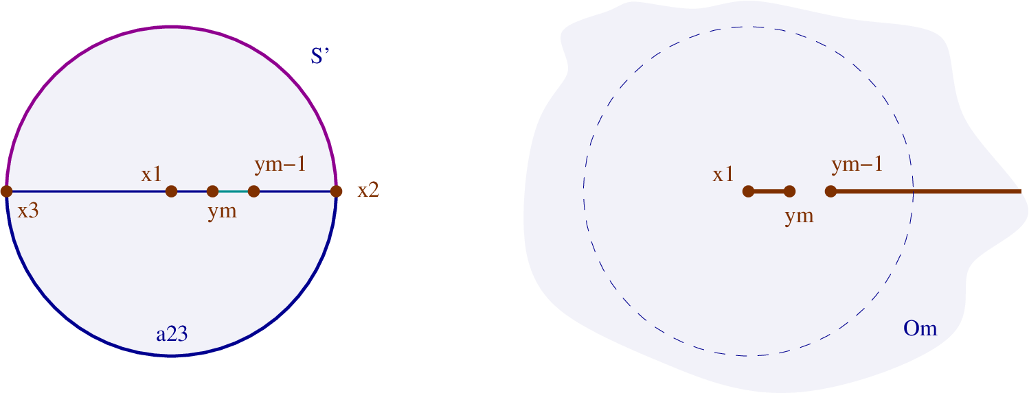
Proof of Lemma A.18.

Let $\mathbb{C}$ with the natural coordinate $w$ be endowed with the standard spherical metric $\left(\frac{2|dw|}{1+|w|^{2}}\right)^{2}$ , for which $\{|w|=1\}$ is a maximal circle. A (multivalued) developing map from $\iota:S\setminus\alpha_{23}\rightarrow\mathbb{C}$ that sends $x_{1}$ to the origin has image equal to the open unit disk and it has order $\vartheta_{1}$ at $x_{1}$ . Thus, there exists a biholomorphism $\psi:S\setminus\alpha_{23}\rightarrow S^{\prime}$ that sends $x_{1}$ to $0$ and such that $\iota=\iota^{\prime}\circ\psi$ , where $\iota^{\prime}(z)=z^{\vartheta_{1}}$ . Moreover $\psi$ can be uniquely chosen so that $x_{2}$ corresponds to $x^{\prime}_{2}=1$ .

Since $[0,1)\subset S^{\prime}$ running from $x^{\prime}_{1}=0$ to $x^{\prime}_{2}=1$ is sent to a geodesic by $\iota^{\prime}$ , such segment corresponds to $\alpha_{12}\subset S$ . Thus the orientation-reversing involution of $S\setminus\alpha_{23}$ that fixes $\alpha_{12}$ must correspond to the conjugation in $S^{\prime}$ and so $x_{3}\in S$ corresponds to $x^{\prime}_{3}=-1$ .

Finally, the point $w_{j}=\tan(\epsilon^{j}/2)$ in $\mathbb{C}$ is at distance $\epsilon^{j}$ from $0$ . Hence, the point $y^{\prime}_{j}=\tan(\epsilon^{j}/2)^{1/\vartheta_{1}}$ in $(0,1)\subset S^{\prime}$ is at distance $\epsilon^{j}$ from $x^{\prime}_{1}=0$ , and so $y^{\prime}_{j}\in S^{\prime}$ corresponds to $y_{j}\in S$ . ∎

We denote by $\dot{S}^{\prime}_{k}$ the punctured domain $S^{\prime}\setminus\{x^{\prime}_{1},x^{\prime}_{2},x^{\prime}_{3},y^{\prime}_{0},\dots,y^{\prime}_{k}\}$ and by $\dot{S}^{\prime}=\dot{S}^{\prime}_{m}$ .

A.2.3 The Strebel differential $\mathpzc{q}_{k}$ on $\dot{S}_{k}$

In order to estimate the extremal lengths in $\dot{S}_{k}$ , consider the Strebel differential $\mathpzc{q}_{k}$ on $\dot{S}_{k}$ associated to $\gamma_{k}$ , such that the total area of $\mathpzc{q}_{k}$ is exactly $\mathrm{Ext}_{\gamma_{k}}(\dot{S}_{k})$ .

Lemma A.19.

The couple $(S,|\mathpzc{q}_{k}|)$ is isomorphic to a doubled rectangle of vertices $x_{1},y_{k},y_{k-1},x_{3}$ with base $x_{1}y_{k}$ of length $\frac{1}{2}\mathrm{Ext}_{\gamma_{k}}(\dot{S}_{k})$ and height $x_{1}x_{3}$ of length $1$ . The horizontal trajectories of $\mathpzc{q}_{k}$ are parallel to the base. The points $y_{k-1},\dots,y_{0},x_{2}$ lie in this order on the horizontal trajectory running from $y_{k-1}$ to $x_{3}$ .

Proof.

The curve $\gamma_{k}$ is essential inside $\hat{S}_{k}=S_{k}\setminus\{x_{1},y_{k},y_{k-1},x_{3}\}$ . Consider the quadratic differential $\widehat{\mathpzc{q}}_{k}$ associated to $\gamma_{k}$ inside $\hat{S}_{k}$ such that $|\widehat{\mathpzc{q}}_{k}|$ has total area $\frac{1}{2}\mathrm{Ext}_{\gamma_{k}}(\dot{S}_{k})$ (see Figure A.2.1 on the right, for the case $k=m$ ). The analysis contained in Example A.12 shows that $\hat{S}_{k}$ is isomorphic to $S_{r,\phi}$ with $\phi=0$ and $r^{2}=\frac{1}{2}\mathrm{Ext}_{\gamma_{k}}(\dot{S}_{k})$ , and so $(\hat{S}_{k},|\widehat{\mathpzc{q}}_{k}|)$ is isometric to a doubled rectangle with corners $x_{1},y_{k},y_{k-1},x_{3}$ . Moreover, the orientation-reversing involution of $\dot{S}_{k}$ is an isometry and so conformal; hence, it fixes the metric $|\widehat{\mathpzc{q}}_{k}|$ and so it is the natural involution of the doubled rectangle. In particular, $\alpha_{12}$ is fixed by the involution of the doubled rectangle and so it is the union of the horizontal segments $x_{1}y_{k}$ and $y_{k-1}x_{3}$ and the vertical segment $y_{k}y_{k-1}$ . It is easy now to check that $\mathpzc{q}_{k}=\widehat{\mathpzc{q}}_{k}$ and the conclusion easily follows. ∎

We call $\mathpzc{q}^{\prime}_{k}$ the corresponding quadratic differential on $\dot{S}^{\prime}_{k}$ and $\gamma^{\prime}_{k}$ the curve in $\dot{S}^{\prime}_{k}$ that corresponds to $\gamma_{k}$ .

A.2.4 Estimate for the extremal length of $\gamma_{k}$ in $\dot{S}_{k}$

The extremal length of $\gamma_{k}\subset\dot{S}_{k}$ is estimated from above using the spherical metric and superadditivity of the modulus. The bound from below uses the plane model of $\dot{S}\setminus\alpha_{23}$ and a classical estimate stating that the modulus of the annulus obtained from $\mathbb{C}$ by removing the two segments $[-1,0]$ and $[t-1,+\infty)$ is at most $\frac{1}{2\pi}\log(16t)$ for all real $t>1$ (see [1, Chap.3B]).

Lemma A.20 (Extremal length of $\gamma_{k}$ ).

The extremal length of $\gamma_{k}$ inside $\dot{S}_{k}$ satisfies

\frac{2\pi\vartheta_{1}}{\vartheta_{1}\log(16)+\log(1/\epsilon)+O(\epsilon)}<\mathrm{Ext}_{\gamma_{k}}(\dot{S}_{k})<\frac{2\pi\vartheta_{1}}{\log(1/\epsilon)}

and so in particular $\displaystyle\mathrm{Ext}_{\gamma_{k}}(\dot{S}_{k})-\frac{2\pi\vartheta_{1}}{\log(1/\epsilon)}=O\left(\frac{\vartheta_{1}^{2}}{\log^{2}(1/\epsilon)}\right)$ .

Proof.

In order to bound $\mathrm{Ext}_{\gamma_{k}}(\dot{S}_{k})$ from below, consider the locus $C_{k}\subset\dot{S}_{k}$ of points at distance between $\epsilon^{k}$ and $\epsilon^{k-1}$ from $x_{1}$ . By Lemma 5.5 we immediately have $M(C_{k})>\frac{1}{2\pi\vartheta_{1}}\log(1/\epsilon)$ and so $\mathrm{Ext}_{\gamma_{k}}(\dot{S}_{k})<\frac{2\pi\vartheta_{1}}{\log(1/\epsilon)}$ .

In order to bound $\mathrm{Ext}_{\gamma_{k}}(\dot{S}_{k})$ from above, consider the quadratic differential $\mathpzc{q}_{k}$ described in Lemma A.19. Since $\alpha_{23}$ is a horizontal segment, $\mathrm{Ext}_{\gamma_{k}}(\dot{S}_{k})=\mathrm{Ext}_{\gamma_{k}}(\dot{S}_{k}\setminus\alpha_{23})=\mathrm{Ext}_{\gamma^{\prime}_{k}}(\dot{S}^{\prime}_{k})$ and it is achieved at the metric $|\mathpzc{q}^{\prime}_{k}|$ . Thus, $\mathrm{Ext}_{\gamma^{\prime}_{k}}(\dot{S}^{\prime}_{k})=\mathrm{Ext}_{\gamma^{\prime}_{k}}\Big(\accentset{\circ}{S}^{\prime}_{k}\setminus\left([0,y^{\prime}_{k}]\cup[y^{\prime}_{k-1},1]\right)\Big)$ . Since $\Omega_{k}=\mathbb{C}\setminus\Big([0,y^{\prime}_{k}]\cup[y^{\prime}_{k-1},+\infty)\Big)$ is biholomorphic to $\mathbb{C}\setminus\left([-1,0]\cup[\frac{y^{\prime}_{k-1}}{y^{\prime}_{k}}-1,+\infty)\right)$ , it follows that

\displaystyle\mathrm{Ext}_{\gamma_{k}}(\dot{S}_{k})^{-1}

\displaystyle=M(\accentset{\circ}{S}^{\prime}_{k}\cap\Omega_{k})<M(\Omega_{k})\leq\frac{1}{2\pi}\log\left(\frac{16y^{\prime}_{k-1}}{y^{\prime}_{k}}\right)<\frac{1}{2\pi}\left(\log(16)+\frac{\log(1/\epsilon)+O(\epsilon)}{\vartheta_{1}}\right)

and so $\displaystyle\mathrm{Ext}_{\gamma_{k}}(\dot{S}_{k})\geq\frac{2\pi\vartheta_{1}}{\vartheta_{1}\log(16)+\log(1/\epsilon)+O(\epsilon)}$ . The last assertion is a straightforward calculation. ∎

A.2.5 Estimate for the extremal systole of $\dot{S}_{k}$

Now we inductively show that the extremal systole of $\dot{S}_{k}$ is realized at the closed curve $\gamma_{k}$ .

Lemma A.21 (Extremal systole of $\dot{S}_{k}$ ).

Suppose that $\varepsilon<\exp\left[-8(4N+1)^{2}\right]$ . Then the extremal systole of the punctured surface $\dot{S}_{k}$ is achieved at $\gamma_{k}$ only.

Proof.

Preliminarly observe that the total area of $S$ for the spherical metric is $2\pi\vartheta_{1}$ and that our assumption on $\varepsilon$ implies that $\log\left(\frac{1}{\epsilon}\right)>8(4N+1)^{2}>\left(\frac{2\pi\vartheta_{1}}{\pi-2}\right)^{2}$ .

Now, $\mathrm{Ext}_{\gamma_{k}}(\dot{S}_{k})<\frac{2\pi\vartheta_{1}}{\log(1/\epsilon)}$ by Lemma A.20. We claim that, if $\gamma\subset\dot{S}_{k}$ is a simple closed curve not homotopic to $\gamma_{k}$ , then $\mathrm{Ext}_{\gamma}(\dot{S}_{k})\geq\frac{2\pi\vartheta_{1}}{\log(1/\epsilon)}$ . It will follow that $\mathrm{Ext}\mathrm{sys}(\dot{S}_{k})$ is attained at $\gamma_{k}$ only.

Denote by $\dot{S}^{+}_{k}$ the region of $\dot{S}_{k}$ consisting of points at $|\mathpzc{q}_{k}|$ -distance less than $\frac{1}{2}$ from the segment $x_{1}y_{k}$ , by $\dot{S}^{-}_{k}$ the region of points at $|\mathpzc{q}_{k}|$ -distance less than $\frac{1}{2}$ from the segment $y_{k-1}x_{3}$ (see Figure A.2.1 on the right in the case $k=m$ ).

Let us prove the above claim by induction on $k\geq 1$ .

Consider the case $k=1$ . The surface $\dot{S}_{1}$ has $5$ punctures $x_{1},x_{2},x_{3},y_{0},y_{1}$ and the only closed curve in $\dot{S}^{+}_{1}$ is $\gamma_{1}$ . A closed curve $\gamma\subset\dot{S}_{1}$ that cannot be deformed inside $\dot{S}^{+}_{1}$ or $\dot{S}^{-}_{1}$ must cross both segments $y_{1}x_{1}$ and $y_{0}x_{3}$ , and so it must have $|\mathpzc{q}_{1}|$ -length at least $2$ . Hence,

\mathrm{Ext}_{\gamma}(\dot{S}_{1})\geq\frac{4}{\mathrm{Ext}_{\gamma_{1}}(\dot{S}_{1})}>\frac{2}{\pi\vartheta_{1}}\log(1/\epsilon)\geq\frac{2\pi\vartheta_{1}}{\log(1/\epsilon)}

where the first inequality on the left follows from the very definition of extremal length using the metric $|\mathpzc{q}_{1}|$ , the second inequality relies on Lemma A.20 and the third inequality is a rephrasing of $\epsilon<\exp(-\vartheta_{1}\pi)$ , which follows from our assumption on $\varepsilon$ .

Finally, a closed curve $\gamma$ contained in $\dot{S}^{-}_{1}$ must be homotopic either to $\gamma_{23}$ that separates $x_{2},x_{3}$ , or to $\gamma_{0,2}$ that separates $y_{0},x_{2}$ or to $\gamma_{0,3}$ that separates $y_{0},x_{3}$ from the other points.

Any curve homotopic to $\gamma_{2,3}$ (resp. $\gamma_{0,2}$ , $\gamma_{0,3}$ ) has spherical length at least $2$ (resp. at least $\pi-2$ , at least $\pi$ ). Hence, $\mathrm{Ext}_{\gamma}(\dot{S}_{1})\geq\frac{(\pi-2)^{2}}{2\pi\vartheta_{1}}$ , which is larger than $\frac{2\pi\vartheta_{1}}{\log(1/\epsilon)}$ by our observation at the very beginning of the proof.

Consider now the case $k>1$ . Again, every simple closed curve in $\dot{S}^{+}_{k}$ is homotopic to $\gamma_{k}$ . Analogously to the case $k=1$ , a simple closed curve $\gamma\subset\dot{S}_{k}$ that is not homotopic to a curve in $\dot{S}^{+}_{k}$ or in $\dot{S}^{-}_{k}$ must have $|\mathpzc{q}_{k}|$ -length at least $2$ and so $\mathrm{Ext}_{\gamma}(\dot{S}_{k})>\frac{2\pi\vartheta_{1}}{\log(1/\epsilon)}$ . Finally, if $\gamma\subset\dot{S}^{-}_{k}$ is a simple closed curve, then $\mathrm{Ext}_{\gamma}(\dot{S}_{k})\geq\mathrm{Ext}_{\gamma}(\dot{S}_{k-1})\geq\frac{2\pi\vartheta_{1}}{\log(1/\epsilon)}$ by induction. ∎

We can now prove the main result of this section.

Proof of Lemma A.17.

First note that $\mathrm{Ext}\mathrm{sys}(\dot{S})=\mathrm{Ext}_{\gamma_{m}}(\dot{S})$ by Lemma A.21, because $\dot{S}=\dot{S}_{m}$ . By taking $N/m$ large enough, the ratio $\frac{\|\text{\boldmath$\vartheta$}\|_{1}}{\vartheta_{1}}>1$ can be made as close to $1$ as desired. Moreover, our assumption on $\varepsilon$ implies that $\frac{\vartheta_{1}}{\log(1/\epsilon)}<\frac{1}{2(4N+1)}$ and so this ratio can be made as small as desired by taking $N$ large enough. Lemma A.20 then ensures that $\mathrm{Ext}_{\gamma_{m}}(\dot{S})$ is as close to $\frac{2\pi\vartheta_{1}}{\log(1/\epsilon)}$ , and so to $\frac{2\pi\|\text{\boldmath$\vartheta$}\|_{1}}{\log(1/\epsilon)}$ , as we wish. ∎

References

[1] Lars V. Ahlfors, Lectures on quasiconformal mappings, second ed., University Lecture Series, vol. 38, American Mathematical Society, Providence, RI, 2006, With supplemental chapters by C. J. Earle, I. Kra, M. Shishikura and J. H. Hubbard. MR 2241787
[2] Enrico Arbarello, Maurizio Cornalba, and Phillip A. Griffiths, Geometry of algebraic curves. Volume II, Grundlehren der Mathematischen Wissenschaften [Fundamental Principles of Mathematical Sciences], vol. 268, Springer, Heidelberg, 2011, With a contribution by Joseph Daniel Harris. MR 2807457
[3] D. Bartolucci and G. Tarantello, Liouville type equations with singular data and their applications to periodic multivortices for the electroweak theory, Comm. Math. Phys. 229 (2002), no. 1, 3–47. MR 1917672
[4] Daniele Bartolucci, Francesca De Marchis, and Andrea Malchiodi, Supercritical conformal metrics on surfaces with conical singularities, Int. Math. Res. Not. IMRN (2011), no. 24, 5625–5643. MR 2863376
[5] Melvyn S. Berger, Riemannian structures of prescribed Gaussian curvature for compact $2$ -manifolds, J. Differential Geometry 5 (1971), 325–332. MR 0295261
[6] Haïm Brezis and Frank Merle, Uniform estimates and blow-up behavior for solutions of $-\Delta u=V(x)e^{u}$ in two dimensions, Comm. Partial Differential Equations 16 (1991), no. 8-9, 1223–1253. MR 1132783
[7] Alessandro Carlotto, On the solvability of singular Liouville equations on compact surfaces of arbitrary genus, Trans. Amer. Math. Soc. 366 (2014), no. 3, 1237–1256. MR 3145730
[8] Chiun-Chuan Chen and Chang-Shou Lin, Mean field equation of Liouville type with singular data: topological degree, Comm. Pure Appl. Math. 68 (2015), no. 6, 887–947. MR 3340376
[9] Subhadip Dey, Spherical metrics with conical singularities on 2-spheres, Geometriae Dedicata (2017), 1–9.
[10] Alexandre Eremenko, Co-axial monodromy, preprint arXiv:1706.04608.
[11] , Metrics of positive curvature with conic singularities on the sphere, Proc. Amer. Math. Soc. 132 (2004), no. 11, 3349–3355 (electronic). MR 2073312 (2005h:53054)
[12] Alexandre Eremenko and Andrei Gabrielov, On metrics of curvature 1 with four conic singularities on tori and on the sphere, Illinois J. Math. 59 (2015), no. 4, 925–947. MR 3628295
[13] Alexandre Eremenko, Andrei Gabrielov, and Vitaly Tarasov, Metrics with four conic singularities and spherical quadrilaterals, Conform. Geom. Dyn. 20 (2016), 128–175. MR 3500744
[14] Alexandre Eremenko and Vitaly Tarasov, Fuchsian equations with three non-apparent singularities, SIGMA Symmetry Integrability Geom. Methods Appl. 14 (2018), 058, 12 pages. MR 3814567
[15] Lisa R. Goldberg, Catalan numbers and branched coverings by the Riemann sphere, Adv. Math. 85 (1991), no. 2, 129–144. MR 1093002
[16] W. K. Hayman, Meromorphic functions, Oxford Mathematical Monographs, Clarendon Press, Oxford, 1964. MR 0164038
[17] John Hamal Hubbard, Teichmüller theory and applications to geometry, topology, and dynamics. Vol. 1, Matrix Editions, Ithaca, NY, 2006, Teichmüller theory, With contributions by Adrien Douady, William Dunbar, Roland Roeder, Sylvain Bonnot, David Brown, Allen Hatcher, Chris Hruska and Sudeb Mitra, With forewords by William Thurston and Clifford Earle. MR 2245223
[18] Michael Kapovich, Branched covers between spheres and polygonal inequalities in simplicial trees, preprint available at https://www.math.ucdavis.edu/ $\sim$ kapovich/EPR/covers.pdf.
[19] Paul Koebe, Über die Uniformisierung beliebiger analytischer Kurven, Göttinger Nachrichten (1907), 191–210.
[20] , Über die Uniformisierung beliebiger analytischer Kurven (Zweite Mitteilung), Göttinger Nachrichten (1907), 633–669.
[21] Chang-Shou Lin and Chin-Lung Wang, Elliptic functions, Green functions and the mean field equations on tori, Ann. of Math. (2) 172 (2010), no. 2, 911–954. MR 2680484
[22] Fu Liu and Brian Osserman, The irreducibility of certain pure-cycle Hurwitz spaces, Amer. J. Math. 130 (2008), no. 6, 1687–1708. MR 2464030
[23] Feng Luo, Monodromy groups of projective structures on punctured surfaces, Invent. Math. 111 (1993), no. 3, 541–555. MR 1202134 (94b:32032)
[24] Feng Luo and Gang Tian, Liouville equation and spherical convex polytopes, Proc. Amer. Math. Soc. 116 (1992), no. 4, 1119–1129. MR 1137227
[25] Rafe Mazzeo and Xuwen Zhu, Conical metrics on Riemann surfaces, I: the compactified configuration space and regularity, preprint arXiv:1710.09781.
[26] Robert C. McOwen, Point singularities and conformal metrics on Riemann surfaces, Proc. Amer. Math. Soc. 103 (1988), no. 1, 222–224. MR 938672 (89m:30089)
[27] Gabriele Mondello and Dmitri Panov, Spherical metrics with conical singularities on a 2-sphere: angle constraints, Int. Math. Res. Not. IMRN (2016), no. 16, 4937–4995. MR 3556430
[28] J. Moser, A sharp form of an inequality by N. Trudinger, Indiana Univ. Math. J. 20 (1970/71), 1077–1092. MR 0301504
[29] Anton Petrunin, Puzzles in geometry which I know and love, preprint arXiv:0906.0290.
[30] Henri Poincaré, Sur l’uniformisation des fonctions analytiques, Acta Math. 31 (1908), no. 1, 1–63. MR 1555036
[31] Inna Scherbak, Rational functions with prescribed critical points, Geom. Funct. Anal. 12 (2002), no. 6, 1365–1380. MR 1952932 (2004c:14101)
[32] Dirk Siersma, Voronoi diagrams and morse theory of the distance function, Geometry in Present Day Science, World Scientific, World Scientific, 1999, pp. 187–208.
[33] Kurt Strebel, Bemerkungen über quadratische Differentiale mit geschlossenen Trajektorien, Ann. Acad. Sci. Fenn. Ser. A I No. 405 (1967), 12. MR 0223564
[34] Marc Troyanov, Les surfaces euclidiennes à singularités coniques, Enseign. Math. (2) 32 (1986), no. 1-2, 79–94. MR 850552 (87i:30079)
[35] , Metrics of constant curvature on a sphere with two conical singularities, Differential geometry (Peñíscola, 1988), Lecture Notes in Math., vol. 1410, Springer, Berlin, 1989, pp. 296–306. MR 1034288 (90m:53057)
[36] , Prescribing curvature on compact surfaces with conical singularities, Trans. Amer. Math. Soc. 324 (1991), no. 2, 793–821. MR 1005085 (91h:53059)

Spherical surfaces with conical points: systole inequality and moduli spaces with many connected components

Abstract

1 Introduction

1.1 Setting

Definition 1.1 (Spherical metric).

Remark 1.2 (Developing map and monodromy representation).

Notation.

Definition 1.3 (Spherical systole).

Definition 1.4 (Extremal systole).

Definition 1.5 (Non-bubbling parameter).

Remark 1.6.

Definition 1.7 (Coaxial representation).

Lemma 9.3 (Coaxial metrics have vanishing non-bubbling parameter).

Notation.

Definition 1.8 (Moduli space of Riemann surfaces).

Definition 1.9 (Moduli space of spherical surfaces).

1.2 Main results

1.2.1 Components of the moduli space of spherical surfaces

Theorem A (Existence of spherical metrics in positive genus).

Remark 1.10.

Theorem B (The moduli space of spherical surfaces can have many components).

Remark 1.11.

1.2.2 Systole inequality and surfaces with one conical point of small angle

Theorem C (Systole inequality).

Theorem D (Non-existence of spherical metrics with one small angle).

Remark 1.12.

Remark 1.13.

Theorem E (Properness of the forgetful map).

1.3 Context and known results

Problem 1.14 (Spherical metrics in a fixed conformal class).

1.3.1 The unpunctured case

1.3.2 Existence of conformal metrics of constant curvature in the subcritical case

Theorem 1.15 (Existence of conformal metrics of constant KK in the subcritical case [36]).

1.3.3 Bubbling phenomenon in positive curvature

Theorem 1.16 (Compactness of the space of spherical metrics in a conformal class [3]).

1.3.4 Existence of conformal spherical metrics in positive genus

Theorem 1.17 (Existence of supercritical spherical metrics in positive genus [4]).

Remark 1.18.

1.3.5 Non-emptyness and connectedness for moduli spaces of spherical surfaces of genus zero

Theorem 1.19 (Monodromy constraints for spherical surfaces of genus zero [27]).

Remark 1.20.

Remark 1.21.

Theorem 1.22 (Connectedness of Hurwitz spaces [22]).

Remark 1.23.

Theorem 1.24 (Spheres with three non-integral angles [14, Theorem 2.5]).

1.3.6 Spherical surfaces with one small angle

Remark 1.25.

Theorem D’ (Image of the forgetful map for small ϑ1\vartheta_{1}).

1.4 Ideas of the proofs of Theorem C and of Theorems D and E

1.4.1 Area estimate for the bubbles

Theorem 9.5.

Corollary 8.12.

Theorem 8.2.

1.4.2 The Voronoi function

1.4.3 Detecting ε\varepsilon-bubbling surfaces

1.4.4 Non-existence for small ϑ1\vartheta_{1} and properness of the forgetful map

1.5 Ideas of the proofs of Theorem A and of Theorem B

1.6 Content of the paper

1.7 Acknowledgements

2 Existence of spherical metrics in positive genus

2.1 Existence of spherical metrics with assigned angles

Theorem 2.1 (Existence of a spherical metric with assigned angles).

Lemma 2.2 (Existence of a spherical metric with one conical point).

Proof.

Lemma 2.3 (Splitting one conical point into 22 conical points).

Proof.

Proposition 2.4 (Splitting one conical point into kk conical points).

Remark 2.5.

Proof of Theorem 2.1.

3 Spherical systole and conical points of small angle

Definition 3.1 (Injectivity and immersion radius at a conical point).

Lemma 3.2 (Diameter estimate for a spherical surface).

Proof.

3.1 Essential curves and injectivity radius

Lemma 3.3 (Geodesic arcs and loops realizing the injectivity radius).

Definition 3.4 (Essential curves, cylinders and loops).

Lemma 3.5 (Essential curves bound the injectivity radius).

Proof.

Lemma 3.6 (Locally isometric immersion νi\nu_{i}).

Proof.

Theorem 1.15 (Existence of conformal metrics of constant $K$ in the subcritical case [36]).

Theorem D’ (Image of the forgetful map for small $\vartheta_{1}$ ).

1.4.3 Detecting $\varepsilon$ -bubbling surfaces

1.4.4 Non-existence for small $\vartheta_{1}$ and properness of the forgetful map

Lemma 2.3 (Splitting one conical point into $2$ conical points).

Proposition 2.4 (Splitting one conical point into $k$ conical points).

Lemma 3.6 (Locally isometric immersion $\nu_{i}$ ).

3.3 Neighbourhood of conical points with angles $\leq 4\pi/3$ and $\leq 2\pi/{3}$

Lemma 3.16 (Existence of conical points close to an arc between $x_{i},x_{j}$ with small $\vartheta_{i}+\vartheta_{j}$ ).

Lemma 4.2 (Upper bound for $\mathcal{V}$ ).

Lemma 4.3 (Finitely many geodesics realize $\mathcal{V}$ ).

Lemma 4.5 ( $\Gamma$ is a finite graph with geodesic edges).

Lemma 4.8 (Convexity of the disks $\bar{D}^{\mathcal{V}}_{x_{i}}$ ).

Corollary 4.9 (Upper bound for the length of level curves of $\mathcal{V}$ ).

Theorem 4.11 (Classification of critical points of $\mathcal{V}$ ).

Lemma 4.12 (Regularity of $\mathcal{V}$ on $\dot{S}\setminus\Gamma$ ).

Lemma 4.13 (Critical points for $\mathcal{V}$ on an edge of $\Gamma$ ).

Lemma 4.15 (Critical values for $\mathcal{V}$ at a vertex of $\Gamma$ ).

Proposition 4.17 (Number of critical values of $\mathcal{V}$ ).

Proposition 4.18 (Delaunay-Morse decomposition of $S$ ).

Lemma 4.21 ( $D^{\mathcal{V}}_{x_{i}}$ and $B^{\max}_{x_{i}}$ at a point $x_{i}$ with small $\vartheta_{i}$ ).