跳到论文正文
W Papers独立论文阅读器 arXiv:1807.04261 论文正文 计算阅读时间 · 0%
引用这篇论文根据当前论文元数据生成,正式投稿前建议核对。


License: arXiv.org perpetual non-exclusive license
arXiv:1807.04261v1 [cs.IT] 11 Jul 2018

Phase Retrieval Under a Generative Prior

Paul Hand Note: Department of Computational and Applied Mathematics, Rice University, Houston, TX    Oscar Leong††footnotemark:    Vladislav Voroninski Note: Helm.ai, Menlo Park, CA
Abstract

The phase retrieval problem asks to recover a natural signal y0∈ℝny_{0}\in\mathbb{R}^{n} from mm quadratic observations, where mm is to be minimized. As is common in many imaging problems, natural signals are considered sparse with respect to a known basis, and the generic sparsity prior is enforced via ℓ1\ell_{1} regularization. While successful in the realm of linear inverse problems, such ℓ1\ell_{1} methods have encountered possibly fundamental limitations, as no computationally efficient algorithm for phase retrieval of a kk-sparse signal has been proven to succeed with fewer than O⁡(k2​log⁡n)O(k^{2}\log n) generic measurements, exceeding the theoretical optimum of O⁡(k​log⁡n)O(k\log n). In this paper, we propose a novel framework for phase retrieval by 1) modeling natural signals as being in the range of a deep generative neural network G:ℝk→ℝnG:\mathbb{R}^{k}\rightarrow\mathbb{R}^{n} and 2) enforcing this prior directly by optimizing an empirical risk objective over the domain of the generator. Our formulation has provably favorable global geometry for gradient methods, as soon as m=O⁡(k​d2​log⁡n)m=O(kd^{2}\log n), where dd is the depth of the network. Specifically, when suitable deterministic conditions on the generator and measurement matrix are met, we construct a descent direction for any point outside of a small neighborhood around the unique global minimizer and its negative multiple, and show that such conditions hold with high probability under Gaussian ensembles of multilayer fully-connected generator networks and measurement matrices. This formulation for structured phase retrieval thus has two advantages over sparsity based methods: 1) deep generative priors can more tightly represent natural signals and 2) information theoretically optimal sample complexity. We corroborate these results with experiments showing that exploiting generative models in phase retrieval tasks outperforms sparse phase retrieval methods.

1 Introduction

We study the problem of recovering a signal y0∈ℝny_{0}\in\mathbb{R}^{n} given m≪nm\ll n phaseless observations of the form b=|A​y0|b=|Ay_{0}| where the measurement matrix A∈ℝm×nA\in\mathbb{R}^{m\times n} is known and |⋅||\cdot| is understood to act entrywise. This is known as the phase retrieval problem. In this work, we assume, as a prior, that the signal y0y_{0} is in the range of a generative model G:ℝk→ℝnG:\mathbb{R}^{k}\rightarrow\mathbb{R}^{n} so that y0=G⁡(x0)y_{0}=G(x_{0}) for some x0∈ℝkx_{0}\in\mathbb{R}^{k}. To recover y0y_{0}, we first recover the original latent code x0x_{0} corresponding to it, from which y0y_{0} is obtained by applying GG. Hence we study the phase retrieval problem under a generative prior:

find​x∈ℝk​such that​b=|A​G​(x)|.\text{find}\ x\in\mathbb{R}^{k}\ \text{such that}\ b=|AG(x)|.

We will refer to this formulation as Deep Phase Retrieval (DPR). The phase retrieval problem has applications in X-ray crystallography [17, 27], optics [32], astronomical imaging [10], diffraction imaging [5], and microscopy [26]. In these problems, the phase information of an object is lost due to physical limitations of scientific instruments. In crystallography, the linear measurements in practice are typically Fourier modes because they are the far field limit of a diffraction pattern created by emitting a quasi-monochromatic wave on the object of interest.

In many applications, the signals to be recovered are compressible or sparse with respect to a certain basis (e.g. wavelets). Many researchers have attempted to leverage sparsity priors in phase retrieval to yield more efficient recovery algorithms [6, 24, 33, 20, 18, 19]. However, these methods have been met with potentially severe fundamental limitations. In the Gaussian measurement regime where AA has i.i.d. Gaussian entries, one would hope that recovery of a kk-sparse nn-dimensional signal is possible with O⁡(k​log⁡n)O(k\log n) measurements. However, there is no known method to succeed with fewer than O⁡(k2​log⁡n)O(k^{2}\log n) measurements. Moreover, [24] proved that the semidefinite program PhaseLift cannot outperform this suboptimal sample complexity by direct ℓ1\ell_{1} penalization. This is in stark contrast to the success of leveraging sparsity in linear compressed sensing to yield optimal sample complexity.

Our contribution.

We establish information theoretically optimal sample complexity11 1 with respect to the dimensionality of the latent code given to the generative network for structured phase retrieval under generic measurements and a novel nonlinear formulation based on empirical risk under a generative prior. In this work, we suppose that the signal of interest is in the range of a generative model. In particular, the generative model is a dd-layer, fully-connected, feed forward neural network with Rectifying Linear Unit (ReLU) activation functions and no bias terms. Let Wi∈ℝni×ni−1W_{i}\in\mathbb{R}^{n_{i}\times n_{i-1}} denote the weights in the ii-th layer of our network for i=1,…,di=1,\dots,d where k=n0<n1<⋯<ndk=n_{0}<n_{1}<\dots<n_{d}. Given an input x∈ℝkx\in\mathbb{R}^{k}, the output of the the generative model G:ℝk→ℝndG:\mathbb{R}^{k}\rightarrow\mathbb{R}^{n_{d}} can be expressed as

G⁡(x):=relu​(Wd​…​relu​(W2​(relu​(W1​x)))​…)\displaystyle G(x):=\text{relu}\left(W_{d}\dots\text{relu}(W_{2}(\text{relu}(W_{1}x)))\dots\right)

where relu​(x)=max⁡(x,0)\text{relu}(x)=\max(x,0) acts entrywise. To recover x0x_{0} from the measurements |A​G​(x0)||AG(x_{0})|, we study the following ℓ2\ell_{2} empirical risk minimization problem:

minx∈ℝk⁡f⁡(x):=12​‖|A​G​(x)|−|A​G​(x0)|‖2.\displaystyle\min_{x\in\mathbb{R}^{k}}f(x):=\frac{1}{2}\left\||AG(x)|-|AG(x_{0})|\right\|^{2}. (1)

We establish a set of deterministic conditions on the generator GG and a measurement matrix AA, which guarantee that the empirical risk formulation has favorable global geometry for gradient methods. We then establish that these deterministic conditions hold with high probability when GG has random Gaussian weights and AA is a Gaussian measurement matrix. Our deterministic conditions likely accommodate other probability distributions on the generator weights and measurement matrices. Moreover, we note that while we assume the weights to have i.i.d. Gaussian entries, we make no assumption about the independence between layers. The Gaussian assumption of the weight matrices is supported by empirical evidence showing neural networks, learned from data, that have weights that obey statistics similar to Gaussians [1]. Furthermore, there has also been work done in establishing a relationship between deep networks and Gaussian processes [23].

Due to the non-convexity of (1), there is no a-priori guarantee that gradient descent schemes can solve (1) as many local minima may exist. In spite of this, our main result illustrates that the objective function exhibits favorable geometry for gradient methods. Moreover, our result holds with information theoretically optimal sample complexity:

Theorem 1 (Informal).

If we have a sufficient number of measurements m=Ω⁡(k​d​log⁡(n1​…​nd))m=\Omega(kd\log(n_{1}\dots n_{d})) and our network is sufficiently expansive at each layer ni=Ω⁡(ni−1​log⁡ni−1)n_{i}=\Omega(n_{i-1}\log n_{i-1}), then there exists a descent direction vx,x0∈ℝkv_{x,x_{0}}\in\mathbb{R}^{k} for any non-zero x∈ℝkx\in\mathbb{R}^{k} outside of two small neighborhoods centered at the true solution x0x_{0} and a negative multiple −ρd​x0-\rho_{d}x_{0} with high probability. In addition, the origin is a local maximum of ff. Here ρd>0\rho_{d}>0 depends on the number of layers dd and ρd→1\rho_{d}\rightarrow 1 as d→∞d\rightarrow\infty.

Our main result asserts that the objective function does not have any spurious local minima or saddle points away from neighborhoods of the true solution and a negative multiple of it. Hence if one were to solve (1) via gradient descent and the algorithm converged, the final iterate would be close to the true solution or a negative multiple of it. The proof of this result is a concentration argument. We first prove the sufficiency of two deterministic conditions on the weights WiW_{i} and measurement matrix AA. We then show that Gaussian WiW_{i} and AA satisfy these conditions with high probability. Finally, using these two conditions, we argue that the specified descent direction vx,x0v_{x,x_{0}} concentrates around a vector hx,x0h_{x,x_{0}} that is continuous for non-zero x∈ℝkx\in\mathbb{R}^{k} and vanishes only when x≈x0x\approx x_{0} or x≈−ρd​x0x\approx-\rho_{d}x_{0}.

Based on our main theoretical result, we also propose a gradient descent scheme to solve (1) in Section 2. We solved phase retrieval tasks on both synthetic and natural signals in Section 4, comparing our algorithm’s results to three sparse phase retrieval methods. Our results corroborate our main theoretical result that recovery with O⁡(k​d2​log⁡n)O(kd^{2}\log n) measurements is possible while outperforming the alternative sparse phase retrieval methods. In particular, our proposed framework is advantageous in allowing enforcement of tighter priors than sparsity, and has information theoretically optimal sample complexity, unlike ℓ1\ell_{1}-based methods.

Prior methodologies for general phase retrieval.

In the Gaussian measurement regime, most of the techniques to solve phase retrieval problems can be classified as convex or non-convex methods. In terms of convex techniques, lifting-based methods transform the signal recovery problem into a rank-one matrix recovery problem by lifting the signal into the space of positive semi-definite matrices. These semidefinite programming (SDP) approaches, such as Phaselift [8], can be provably recover any nn-dimensional signal with O⁡(n​log⁡n)O(n\log n) measurements. Other convex methods include PhaseCut [31], an SDP approach, and linear programming algorithms such as PhaseMax [13]

Non-convex methods encompass alternating minimization approaches such as the original Gerchberg-Saxton [12] and Fienup [11] algorithms and direct optimization algorithms such as Wirtinger Flow [7]. These latter methods directly tackle the least squares objective function:

miny∈ℝn⁡12​‖|A​y|2−|A​y0|2‖2.\displaystyle\min_{y\in\mathbb{R}^{n}}\frac{1}{2}\left\||Ay|^{2}-|Ay_{0}|^{2}\right\|^{2}. (2)

In the seminal work, [7] show that through an initialization via the spectral method, a gradient descent scheme can solve (2) where the gradient is understood in the sense of Wirtinger calculus with O⁡(n​log⁡n)O(n\log n) measurements. Expanding on this, a later study on the minimization of (2) in [29] showed that with O⁡(n​log3​n)O(n\log^{3}n) measurements, the energy landscape of the objective function exhibited global benign geometry which would allow it to be solved efficiently by gradient descent schemes without special initialization. There also exist amplitude flow methods that solve the following non-smooth variation of (2):

miny∈ℝn⁡12​‖|A​y|−|A​y0|‖2.\displaystyle\min_{y\in\mathbb{R}^{n}}\frac{1}{2}\left\||Ay|-|Ay_{0}|\right\|^{2}. (3)

These methods have found success with only O⁡(n)O(n) measurements [9] and have shown to empirically perform better than intensity-based methods using the squared formulation in (2) [36].

Sparse phase retrieval.

Many of the successful methodologies for general phase retrieval have been adapted to try to solve sparse phase retrieval problems. In terms of non-convex optimization, wirtinger flow type methods such as Thresholded Wirtinger Flow [6] create a sparse initializer via the spectral method and perform thresholded gradient descent updates to generate sparse iterates to solve (2). Another non-convex method, SPARTA [33], estimates the support of the signal for its initialization and performs hard thresholded gradient updates to the amplitude-based objective function (3). Both of these methods require O⁡(k2​log⁡n)O(k^{2}\log n) measurements for a generic kk-sparse nn-dimensional signal to succeed, which is more than the theoretical optimum O⁡(k​log⁡n)O(k\log n).

While lifting-based methods such as Phaselift have been proven unable to beat the suboptimal sample complexity O⁡(k2​log⁡n)O(k^{2}\log n), there has been some progress towards breaking this barrier. In [15], the authors show that with an initializer that sufficiently correlates with the true solution, a linear program can recover the sparse signal from O⁡(k​log⁡nk)O(k\log\frac{n}{k}) measurements. However, the best known initialization methods require at least O⁡(k2​log⁡n)O(k^{2}\log n) measurements [6]. Outside of the Gaussian measurement regime, there have been other results showing that if one were able to design their own measurement matrices, then the optimal sample complexity could be reached [18]. For example, [2] showed that assuming the measurement vectors were chosen from an incoherent subspace, then recovery is possible with O⁡(k​log⁡nk)O(k\log\frac{n}{k}) measurements. However, these results would be difficult to generalize to the experimental setting as their design architectures are often unrealistic. Moreover, the Gaussian measurement regime more closely models the experimental Fourier diffraction measurements observed in, for example, X-ray crystallography. As Fourier models are the ultimate goal, results towards lowering this sample complexity in the Gaussian measurement regime must be made or new modes of regularization must be explored in order for the theory and practice of phase retrieval to advance.

Related work.

There has been recent empirical evidence supporting applying a deep learning based approach to holographic imaging, a phase retrieval problem. The authors in [14] show that a neural network with ReLU activation functions can learn to perform holographic image reconstruction. In particular, they show that compared to current approaches, this neural network based method requires less measurements to succeed and is computationally more efficient, needing only one hologram to reconstruct the necessary images.

Furthermore, there have been a number of recent advancements in leveraging generative priors over sparsity priors in compressed sensing. In [4], the authors considered the least squares objective:

minx∈ℝk⁡12​‖A​G​(x)−A​G​(x0)‖2.\displaystyle\min_{x\in\mathbb{R}^{k}}\frac{1}{2}\|AG(x)-AG(x_{0})\|^{2}. (4)

They provided empirical evidence showing that 5-10X fewer measurements were needed to succeed in recovery compared to standard sparsity-based approaches such as Lasso. In terms of theory, they showed that if AA satisfied a restricted eigenvalue condition and if one were able to solve (4), then the solution would be close to optimal. The authors in [16] analyze the same optimization problem as in [4] but establish global theoretical guarantees regarding the non-convex objective function. Under particular conditions about the expansivity of each neural network layer and randomness assumptions on their weights, they show that the energy landscape of the objective function does not have any spurious local minima. Furthermore, they show that there is always a descent direction outside of two small neighborhoods of the global minimum and a negative scalar multiple of it. The success of leveraging generative priors in compressed sensing along with the sample complexity bottlenecks in sparse phase retrieval have influenced this work to consider enforcing a generative prior in phase retrieval to surpass sparse phase retrieval’s current theoretical and practical limitations.

1.1 Notation

Let (⋅)⊤(\cdot)^{\top} denote the real transpose. Let [n]={1,…,n}[n]=\{1,\dots,n\}. Let 𝟙S\operatorname{\mathbbm{1}}_{S} denote the indicator function on the set SS. For a vector v∈ℝnv\in\mathbb{R}^{n}, diag​(v>0)\text{diag}(v>0) is 11 in the ii-th diagonal entry if vi>0v_{i}>0 and 00 otherwise. Let ℬ⁡(x,r)\mathcal{B}(x,r) denote the Euclidean ball centered at xx with radius rr. Let ∥⋅∥\|\cdot\| denote the ℓ2\ell_{2} norm for vectors and spectral norm for matrices. For any non-zero x∈ℝnx\in\mathbb{R}^{n}, let x^=x/‖x‖\hat{x}=x/\|x\|. Let Πi=d1​Wi=Wd​Wd−1​…​W1\Pi_{i=d}^{1}W_{i}=W_{d}W_{d-1}\dots W_{1}. Let InI_{n} be the n×nn\times n identity matrix. Let Sk−1S^{k-1} denote the unit sphere in ℝk\mathbb{R}^{k}. We write c=Ω⁡(δ)c=\Omega(\delta) when c≥C​δc\geq C\delta for some positive constant CC. Similarly, we write c=O⁡(δ)c=O(\delta) when c≤C​δc\leq C\delta for some positive constant CC. When we say that a constant depends polynomially on ϵ−1\epsilon^{-1}, this means that it is at least C​ϵ−kC\epsilon^{-k} for some positive CC and positive integer kk. For notational convenience, we write a=b+O1​(ϵ)a=b+O_{1}(\epsilon) if ‖a−b‖≤ϵ\|a-b\|\leq\epsilon where ∥⋅∥\|\cdot\| denotes |⋅||\cdot| for scalars, ℓ2\ell_{2} norm for vectors, and spectral norm for matrices. Define sgn:ℝ→ℝ\operatorname{sgn}:\mathbb{R}\rightarrow\mathbb{R} to be sgn⁡(x)=x/|x|\operatorname{sgn}(x)=x/|x| for non-zero x∈ℝx\in\mathbb{R} and sgn⁡(x)=0\operatorname{sgn}(x)=0 otherwise. For a vector v∈ℝnv\in\mathbb{R}^{n}, diag​(sgn⁡(v))\text{diag}(\operatorname{sgn}(v)) is sgn⁡(vi)\operatorname{sgn}(v_{i}) in the ii-th diagonal entry. Let g∘dg^{\circ d} denote the composition of a function gg with itself dd times.

2 Algorithm

While our main result illustrates that the objective function exhibits favorable geometry for optimization, it does not guarantee recovery of the signal as gradient descent algorithms could, in principle, converge to the negative multiple of our true solution. Hence we propose a gradient descent scheme to recover the desired solution by escaping this region. First, consider Figure 1 which illustrates the behavior of our objective function in expectation, i.e. when the number of measurements m→∞m\rightarrow\infty.

Refer to caption
Figure 1: Energy landscape of (1) with m→∞m\rightarrow\infty and true solution x0=[1, 0]⊤∈ℝ2x_{0}=\left[1,\ 0\right]^{\top}\in\mathbb{R}^{2}.

We observe two important attributes of the objective function’s landscape: 1) there exist two minima, the true solution x0x_{0} and a negative multiple −β​x0-\beta x_{0} for some β>0\beta>0 and 2) if z≈x0z\approx x_{0} while w≈−β​x0w\approx-\beta x_{0}, we have that f⁡(z)<f⁡(w)f(z)<f(w), i.e. the objective function value is lower near the true solution than near its negative multiple. This is due to the fact that the true solution is in fact the global optimum.

Based on these attributes, we will introduce a gradient descent scheme to converge to the global minimum. First, we define some useful quantities. For any x∈ℝkx\in\mathbb{R}^{k} and matrix W∈ℝn×kW\in\mathbb{R}^{n\times k}, define W+,x:=diag​(W​x>0)​W.W_{+,x}:=\text{diag}(Wx>0)W. That is, W+,xW_{+,x} keeps the rows of WW that have a positive dot product with xx and zeroes out the rows that do not. We will extend the definition of W+,xW_{+,x} to each layer of weights WiW_{i} in our neural network. For W1∈ℝn1×kW_{1}\in\mathbb{R}^{n_{1}\times k} and x∈ℝkx\in\mathbb{R}^{k}, define W1,+,x:=diag​(W1​x>0)​W1.W_{1,+,x}:=\text{diag}(W_{1}x>0)W_{1}. For each layer i∈[d]i\in[d], define

Wi,+,x:=diag​(Wi​Wi−1,+,x​…​W2,+,x​W1,+,x​x>0)​Wi.W_{i,+,x}:=\text{diag}(W_{i}W_{i-1,+,x}\dots W_{2,+,x}W_{1,+,x}x>0)W_{i}.

Wi,+,xW_{i,+,x} keeps the rows of WiW_{i} that are active when the input to the generative model is xx. Then, for any x∈ℝkx\in\mathbb{R}^{k}, the output of our generative model can be written as G⁡(x)=(Πi=d1​Wi,+,x)​x.G(x)=(\Pi_{i=d}^{1}W_{i,+,x})x. For any z∈ℝnz\in\mathbb{R}^{n}, define Az:=diag​(sgn⁡(A​z))​A.A_{z}:=\text{diag}(\operatorname{sgn}(Az))A. Note that |A​G​(x)|=AG⁡(x)​G​(x)|AG(x)|=A_{G(x)}G(x) for any x∈ℝkx\in\mathbb{R}^{k}.

Since a gradient descent scheme could in principle be attracted to the negative multiple, we exploit the geometry of the objective function’s landscape to escape this region. First, choose a random initial iterate for gradient descent x1≠0x_{1}\neq 0. At each iteration i=1,2,…i=1,2,\dots, compute the descent direction

vxi,x0:=(Πi=d1​Wi,+,xi)⊤​AG⁡(xi)⊤​(|A​G​(xi)|−|A​G​(x0)|).\displaystyle v_{x_{i},x_{0}}:=(\Pi_{i=d}^{1}W_{i,+,x_{i}})^{\top}A_{G(x_{i})}^{\top}\left(|AG(x_{i})|-|AG(x_{0})|\right).

This is the gradient of our objective function ff where ff is differentiable. Once computed, we then take a step in the direction of −vxi,x0-v_{x_{i},x_{0}}. However, prior to taking this step, we compare the objective function value for xix_{i} and its negation −xi-x_{i}. If f⁡(−xi)<f⁡(xi)f(-x_{i})<f(x_{i}), then we set xix_{i} to its negation, compute the descent direction and update the iterate. The intuition for this algorithm relies on the landscape illustrated in Figure 1: since the true solution x0x_{0} is the global minimum and −ρd​x0-\rho_{d}x_{0} is a local minimum, the objective function value near x0x_{0} is smaller than near −ρd​x0-\rho_{d}x_{0}. Hence if we begin to converge towards −ρd​x0-\rho_{d}x_{0}, this algorithm will escape this region by choosing the point with lower objective function value, which will be in a neighborhood of x0x_{0}. Algorithm 1 formally outlines this process.

Algorithm 1 Deep Phase Retrieval (DPR) Gradient method
0:  Weights WiW_{i}, measurement matrix AA, observations |A​G​(x0)||AG(x_{0})|, and step size α>0\alpha>0
1:  Choose an arbitrary initial point x1∈ℝk∖{0}x_{1}\in\mathbb{R}^{k}\setminus\{0\}
2:  for i=1,2,…i=1,2,\ldots do
3:   if f⁡(−xi)<f⁡(xi)f(-x_{i})<f(x_{i}) then
4:    xi←−xix_{i}\leftarrow-x_{i};
5:   end if
6:   Compute vxi,x0=(Πi=d1​Wi,+,xi)⊤​AG⁡(xi)⊤​(|A​G​(xi)|−|A​G​(x0)|)v_{x_{i},x_{0}}=(\Pi_{i=d}^{1}W_{i,+,x_{i}})^{\top}A_{G(x_{i})}^{\top}\left(|AG(x_{i})|-|AG(x_{0})|\right)
7:   xi+1=xi−α​vxi,x0x_{i+1}=x_{i}-\alpha v_{x_{i},x_{0}}
8:  end for

Remark.

We would like to note an important distinction between the landscape observed in general phase retrieval and our formulation. In general phase retrieval, there is an inherent ambiguity in the measurements |A​y0||Ay_{0}| as both y0y_{0} and −y0-y_{0} solve (2) and (3). In the complex case, there are even a continuum of solutions as ei​ϕ​y0e^{i\phi}y_{0} is a solution for any ϕ∈[0,2​π]\phi\in[0,2\pi]. In our scenario, the generative model GG introduces a nonlinearity that resolves this ambiguity in two ways. First, due to its injectivity: if y0=G⁡(x0)y_{0}=G(x_{0}) for some x0∈ℝkx_{0}\in\mathbb{R}^{k}, then x0x_{0} is in fact the global optimum to (1). Second, as an added benefit, the non-negativity of GG naturally resolves the sign ambiguity since −y0∉range​(G)-y_{0}\notin\text{range}(G). While these properties certainly aid our analysis, they do not trivialize the matter as the nonlinearity of GG must still be handled with care.

3 Main Theoretical Analysis

We now formally present our main result. While the objective function is not smooth, it’s one-sided directional derivatives exist everywhere due to the piecewise linearity of GG. Let Dv​f​(x)D_{v}f(x) denote the unnormalized one-sided directional derivative of ff at xx in the direction vv: Dv​f​(x)=limt→0+f⁡(x+t​v)−f⁡(x)t.D_{v}f(x)=\lim_{t\rightarrow 0^{+}}\frac{f(x+tv)-f(x)}{t}. Note that we make no assumption about the independence between layers.

Theorem 2.

Fix ϵ>0\epsilon>0 such that K1​d8​ϵ1/4≤1K_{1}d^{8}\epsilon^{1/4}\leq 1 and let d≥2d\geq 2. Suppose that GG is such that WiW_{i} has i.i.d. 𝒩⁡(0,1/ni)\mathcal{N}(0,1/n_{i}) entries for i=1,…,di=1,\dots,d. Suppose that AA has i.i.d. 𝒩⁡(0,1/m)\mathcal{N}(0,1/m) entries. If m≥c​d​k​log⁡(n1​n2​…​nd)m\geq cdk\log(n_{1}n_{2}\dots n_{d}) and ni≥c​ni−1​log⁡ni−1n_{i}\geq cn_{i-1}\log n_{i-1} for i=1,…,di=1,\dots,d, then with probability at least 1−∑i=1dc~​ni​e−γ​ni−1−γ~​m4​k​e−C​m1-\sum_{i=1}^{d}\tilde{c}n_{i}e^{-\gamma n_{i-1}}-\tilde{\gamma}m^{4k}e^{-Cm}, the following holds: for all non-zero x,x0∈ℝkx,x_{0}\in\mathbb{R}^{k}, there exists vx,x0∈ℝkv_{x,x_{0}}\in\mathbb{R}^{k} such that the one-sided directional derivatives of ff satisfy

D−vx,x0​f​(x)<0,\displaystyle D_{-v_{x,x_{0}}}f(x)<0,\ ∀x∉ℬ⁡(x0,K2​d3​ϵ1/4​‖x0‖)∪ℬ⁡(−ρd​x0,K2​d14​ϵ1/4​‖x0‖)∪{0},\displaystyle\ \forall x\notin\mathcal{B}(x_{0},K_{2}d^{3}\epsilon^{1/4}\|x_{0}\|)\cup\mathcal{B}(-\rho_{d}x_{0},K_{2}d^{14}\epsilon^{1/4}\|x_{0}\|)\cup\{0\},
Dx​f​(0)<0,\displaystyle D_{x}f(0)<0,\ ∀x≠0,\displaystyle\ \forall x\neq 0,

where ρd>0\rho_{d}>0 converges to 11 as d→∞d\rightarrow\infty and K1K_{1} and K2K_{2} are universal constants. Here cc and γ−1\gamma^{-1} depend polynomially on ϵ−1\epsilon^{-1}, CC depends on ϵ\epsilon, and c~\tilde{c} and γ~\tilde{\gamma} are universal constants.

The result will be shown by proving the sufficiency of two deterministic conditions on the weights WiW_{i} of our generative network and the measurement matrix AA.

Weight Distribution Condition.

The first condition quantifies the Gaussianity and spatial arrangement of the neurons in each layer. We say that WW satisfies the Weight Distribution Condition (WDC) with constant ϵ>0\epsilon>0 if for any non-zero x,y∈ℝkx,y\in\mathbb{R}^{k}:

‖W+,x⊤​W+,y−Qx,y‖≤ϵ​where​Qx,y:=π−θx,y2​π​Ik+sin⁡θx,y2​π​Mx^↔y^.\displaystyle\left\|W_{+,x}^{\top}W_{+,y}-Q_{x,y}\right\|\leq\epsilon\ \text{where}\ Q_{x,y}:=\frac{\pi-\theta_{x,y}}{2\pi}I_{k}+\frac{\sin\theta_{x,y}}{2\pi}M_{\hat{x}\leftrightarrow\hat{y}}.

Here θx,y=∠⁡(x,y)\theta_{x,y}=\angle(x,y) and Mx^↔y^M_{\hat{x}\leftrightarrow\hat{y}} is the matrix that sends x^↦y^\hat{x}\mapsto\hat{y}, y^↦x^\hat{y}\mapsto\hat{x}, and z↦0z\mapsto 0 for any z∈span​({x,y})⟂z\in\text{span}(\{x,y\})^{\perp}. If Wi,j∼𝒩⁡(0,1/n)W_{i,j}\sim\mathcal{N}(0,1/n), then an elementary calculation gives 𝔼⁡[W+,x⊤​W+,y]=Qx,y\operatorname{\mathbb{E}}\left[W_{+,x}^{\top}W_{+,y}\right]=Q_{x,y}. [16] proved that Gaussian WW satisfies the WDC with high probability (Lemma 1 in Appendix).

Range Restricted Concentration Property.

The second condition is similar in the sense that it quantifies whether the measurement matrix behaves like a Gaussian when acting on the difference of pairs of vectors given by the output of the generative model. We say that A∈ℝm×nA\in\mathbb{R}^{m\times n} satisfies the Range Restricted Concentration Property (RRCP) with constant ϵ>0\epsilon>0 if for all non-zero x,y∈ℝkx,y\in\mathbb{R}^{k}, the matrices AG⁡(x)A_{G(x)} and AG⁡(y)A_{G(y)} satisfy the following for all x1,x2,x3,x4∈ℝkx_{1},x_{2},x_{3},x_{4}\in\mathbb{R}^{k}:

|⟨(AG⁡(x)⊤AG⁡(y)−ΦG⁡(x),G⁡(y))(G(x1)−G(x2)),\displaystyle|\langle(A_{G(x)}^{\top}A_{G(y)}-\Phi_{G(x),G(y)})(G(x_{1})-G(x_{2})), G(x3)−G(x4)⟩|\displaystyle G(x_{3})-G(x_{4})\rangle|
≤7​ϵ​‖G⁡(x1)−G⁡(x2)‖​‖G⁡(x3)−G⁡(x4)‖\displaystyle\leq 7\epsilon\|G(x_{1})-G(x_{2})\|\|G(x_{3})-G(x_{4})\|

where

Φz,w:=π−2​θz,wπ​In+2sinθz,wπ​Mz^↔w^.\displaystyle\Phi_{z,w}:=\frac{\pi-2\theta_{z,w}}{\pi}I_{n}+\frac{2\sin\theta_{z,w}}{\pi}M_{\hat{z}\leftrightarrow\hat{w}}.

If Ai,j∼𝒩⁡(0,1/m)A_{i,j}\sim\mathcal{N}(0,1/m), then for any z,w∈ℝnz,w\in\mathbb{R}^{n}, a similar calculation for Gaussian WW gives 𝔼⁡[Az⊤​Aw]=Φz,w\operatorname{\mathbb{E}}\left[A_{z}^{\top}A_{w}\right]=\Phi_{z,w}. In our work, we establish that Gaussian AA satisfies the RRCP with high probability. Please see Section 5.3 in the Appendix for a complete proof.

We emphasize that these two conditions are deterministic, meaning that our results could extend to non-Gaussian distributions. We now state our main deterministic result:

Theorem 3.

Fix ϵ>0\epsilon>0 such that K1​d8​ϵ1/4≤1K_{1}d^{8}\epsilon^{1/4}\leq 1 and let d≥2d\geq 2. Suppose that GG is such that WiW_{i} satisfies the WDC with constant ϵ\epsilon for all i=1,…,di=1,\dots,d. Suppose A∈ℝm×ndA\in\mathbb{R}^{m\times n_{d}} satisfies the RRCP with constant ϵ\epsilon. Then the same conclusion as Theorem 2 holds.

3.1 Proof sketch for Theorem 2

Before we outline the proof of Theorem 2, we specify the descent direction vx,x0v_{x,x_{0}}. For any x∈ℝkx\in\mathbb{R}^{k} where ff is differentiable, we have that

∇f​(x)=(Πi=d1​Wi,+,x)⊤​A⊤​A​(Πi=d1​Wi,+,x)​x−(Πi=d1​Wi,+,x)⊤​AG⁡(x)⊤​AG⁡(x0)​(Πi=d1​Wi,+,x0)​x0.\displaystyle\nabla f(x)=(\Pi_{i=d}^{1}W_{i,+,x})^{\top}A^{\top}A(\Pi_{i=d}^{1}W_{i,+,x})x-(\Pi_{i=d}^{1}W_{i,+,x})^{\top}A_{G(x)}^{\top}A_{G(x_{0})}(\Pi_{i=d}^{1}W_{i,+,x_{0}})x_{0}.

This is precisely the descent direction specified in DPR, expanded with our notation. When ff is not differentiable at xx, choose a direction ww such that ff is differentiable at x+δ​wx+\delta w for sufficiently small δ>0\delta>0. Such a direction ww exists by the piecewise linearity of the generative model GG. Hence we define our descent direction vx,x0v_{x,x_{0}} as

vx,x0={∇f​(x)f​differentiable at ​x∈ℝklimδ→0+∇f​(x+δ​w)otherwise.\displaystyle v_{x,x_{0}}=\begin{cases}\nabla f(x)&f\ \text{differentiable at }x\in\mathbb{R}^{k}\\ \lim_{\delta\rightarrow 0^{+}}\nabla f(x+\delta w)&\text{otherwise.}\end{cases}

For non-zero x,x0∈ℝkx,x_{0}\in\mathbb{R}^{k}, let θ0=∠⁡(x,x0)\theta_{0}=\angle(x,x_{0}). To understand how the map x↦relu​(W​x)x\mapsto\text{relu}(Wx) distorts angles in expectation, define g:ℝ→ℝg:\mathbb{R}\rightarrow\mathbb{R} by

g⁡(θ)=cos−1⁡(cos⁡θ⁡(π−θ)+sin⁡θπ).g(\theta)=\cos^{-1}\left(\frac{\cos\theta(\pi-\theta)+\sin\theta}{\pi}\right).

Then for i≥1i\geq 1, set θ¯i=g⁡(θ¯i−1)\overline{\theta}_{i}=g(\overline{\theta}_{i-1}) where θ¯0=θ0\overline{\theta}_{0}=\theta_{0}. The following is a sketch of the proof of Theorem 2:

  • •

    By the WDC and RRCP, we have that the descent direction vx,x0v_{x,x_{0}} concentrates around a particular vector v¯x,x0\overline{v}_{x,x_{0}} defined by

    v¯x,x0\displaystyle\overline{v}_{x,x_{0}} :=(Πi=d1​Wi,+,x)⊤​(Πi=d1​Wi,+,x)​x−(Πi=d1​Wi,+,x)⊤​ΦG⁡(x),G⁡(x0)​(Πi=d1​Wi,+,x0)​x0.\displaystyle:=(\Pi_{i=d}^{1}W_{i,+,x})^{\top}(\Pi_{i=d}^{1}W_{i,+,x})x-(\Pi_{i=d}^{1}W_{i,+,x})^{\top}\Phi_{G(x),G(x_{0})}(\Pi_{i=d}^{1}W_{i,+,x_{0}})x_{0}.
  • •

    The WDC establishes that v¯x,x0\overline{v}_{x,x_{0}} concentrates uniformly for all non-zero x,x0∈ℝkx,x_{0}\in\mathbb{R}^{k} around a continuous vector hx,x0h_{x,x_{0}} defined by

    hx,x0\displaystyle h_{x,x_{0}} :=−‖x0‖2d​(π−2​θ¯dπ)​(∏i=0d−1π−θ¯iπ)​x^0\displaystyle:=-\frac{\|x_{0}\|}{2^{d}}\left(\frac{\pi-2\overline{\theta}_{d}}{\pi}\right)\left(\prod_{i=0}^{d-1}\frac{\pi-\overline{\theta}_{i}}{\pi}\right)\hat{x}_{0}
    +12d​[‖x‖−‖x0‖​(2sinθ¯dπ−(π−2​θ¯dπ)​∑i=0d−1sin⁡θ¯iπ​(∏j=i+1d−1π−θ¯iπ))]​x^.\displaystyle+\frac{1}{2^{d}}\left[\|x\|-\|x_{0}\|\left(\frac{2\sin\overline{\theta}_{d}}{\pi}-\left(\frac{\pi-2\overline{\theta}_{d}}{\pi}\right)\sum_{i=0}^{d-1}\frac{\sin\overline{\theta}_{i}}{\pi}\left(\prod_{j=i+1}^{d-1}\frac{\pi-\overline{\theta}_{i}}{\pi}\right)\right)\right]\hat{x}.

    This holds uniformly for all non-zero x,x0∈ℝkx,x_{0}\in\mathbb{R}^{k}.

  • •

    A direct analysis shows that hx,x0h_{x,x_{0}} is only small in norm for x≈x0x\approx x_{0} and x≈−ρd​x0x\approx-\rho_{d}x_{0}. See section 5.2 for a complete proof. Since vx,x0≈v¯x,x0≈hx,x0v_{x,x_{0}}\approx\overline{v}_{x,x_{0}}\approx h_{x,x_{0}}, vx,x0v_{x,x_{0}} is also only small in norm in neighborhoods around x0x_{0} and −ρd​x0-\rho_{d}x_{0}, establishing Theorem 3.

  • •

    Gaussian WiW_{i} and AA satisfy the WDC and RRCP with high probability (Lemma 1 and Proposition 2 in Appendix).

Theorem 2 is a combination of Lemma 1, Proposition 2, and Theorem 3. The full proofs of these results can be found in the Appendix.

4 Numerical Experiments

In this section, we investigate the use of enforcing generative priors on phase retrieval tasks. We used the proposed DPR Gradient Method (Algorithm 1) and compared our results with three sparse phase retrieval algorithms: the sparse truncated amplitude flow algorithm (SPARTA) [33], Thresholded Wirtinger Flow (TWF) [6], and the alternating minimization algorithm CoPRAM [19]. For the remainder of this section, we will refer to the DPR Gradient Method as DPR.

4.1 Experiments for Gaussian signals

We first consider synthetic experiments using Gaussian measurements on Gaussian signals. In particular, we considered a two layer network given by G⁡(x)=relu​(W2​relu​(W1​x))G(x)=\text{relu}(W_{2}\text{relu}(W_{1}x)) where each WiW_{i} has i.i.d. 𝒩⁡(0,1)\mathcal{N}(0,1) entries for i=1,2i=1,2. We set k=10k=10, n1=500n_{1}=500, and n2=1000n_{2}=1000. We let the entries of A∈ℝm×n2A\in\mathbb{R}^{m\times n_{2}} and x0∈ℝkx_{0}\in\mathbb{R}^{k} be i.i.d. 𝒩⁡(0,1)\mathcal{N}(0,1). We ran DPR for 2525 random instances of (A,W1,W2,x0)(A,W_{1},W_{2},x_{0}). A reconstruction x⋆x^{\star} is considered successful if the relative error ‖x⋆−x0‖/‖x0‖≤10−4\|x^{\star}-x_{0}\|/\|x_{0}\|\leq 10^{-4}. We also compared our results with SPARTA, TWF, and CoPRAM. In this setting, we chose a k=10k=10-sparse y0∈ℝn2y_{0}\in\mathbb{R}^{n_{2}}, where the nonzero coefficients are i.i.d. 𝒩⁡(0,1)\mathcal{N}(0,1). As before, we ran each algorithm with 2525 random instances of (A,y0)(A,y_{0}). Figure 2 displays the percentage of successful trials for different ratios m/nm/n where n=n2=1000n=n_{2}=1000 and mm is the number of measurements. Since SPARTA was the most successful amongst the sparse methods, we also experimented with lower sparsity levels k=3,5k=3,5. We note that DPR achieves nearly the same empirical success rate of recovering a 1010-dimensional latent code as SPARTA in recovering a 33-sparse 10001000-dimensional signal. For more comparable sparsity levels to the latent code dimension, DPR outperforms each alternative method with far fewer measurements.

Refer to caption
Refer to caption
Figure 2: Empirical success rate with ratios m/nm/n where n=1000n=1000 with DPR’s latent code dimension set to k=10.k=10. The sparsity level for each recovery algorithm is initially set to k=10k=10 (top) while we experiment with SPARTA’s sparsity levels from k=3,5,10k=3,5,10 (bottom).

4.2 Experiments for MNIST and CelebA

We next consider image recovery tasks, where we use two different generative models for the MNIST and CelebA datasets. In each task, the goal is to recover an image y0y_{0} given |A​y0||Ay_{0}| where A∈ℝm×nA\in\mathbb{R}^{m\times n} has i.i.d. 𝒩⁡(0,1/m)\mathcal{N}(0,1/m) entries. We found an estimate image G⁡(x⋆)G(x^{\star}) in the range of our generator via gradient descent, using the Adam optimizer [21]. Empirically, we noticed that DPR would typically only negate the latent code (Lines 3–4) at the initial iterate, if necessary. Hence we use a modified version of DPR in these image experiments: we ran two sessions of gradient descent for a random initial iterate x1x_{1} and its negation −x1-x_{1} and chose the most successful reconstruction.

In the first image experiment, we used a pretrained Variational Autoencoder (VAE) from [4] that was trained on the MNIST dataset [22]. This dataset consists of 60,00060,000 28×2828\times 28 images of handwritten digits. As described in [4], the recognition network is of size 784−500−500−20784-500-500-20 while the generator network is of size 20−500−500−78420-500-500-784. The latent code space dimension is k=20k=20.

For the sparse phase retrieval methods, we performed sparse recovery by transforming the images using the Daubechies-4 Wavelet Transform. More specifically, we considered the vector of wavelet coefficients v0=Ψ​y0v_{0}=\Psi y_{0} which is compressible. Since the wavelet transform Ψ\Psi is orthogonal and the measurement matrix AA is Gaussian, A​Ψ⊤A\Psi^{\top} and AA are equal in distribution due to the rotational invariance of AA. Hence, instead of recovering v0v_{0} from measurements |A​y0|=|A​Ψ⊤​v0||Ay_{0}|=|A\Psi^{\top}v_{0}|, we recover v0v_{0} from |A​v0||Av_{0}|. We then take an inverse wavelet transform to retrieve the approximate image. To appropriately take the wavelet transform, we pad the images with zeros uniformly around the border so that they are of size 32×3232\times 32. If a sparse recovery algorithm required a sparsity parameter, we ran the algorithm with a range of sparsity parameter values, choosing the best reconstruction in terms of lowest reconstruction error. The resulting images generated by our algorithm were also uniformly padded with zeros around the border to obtain 32×3232\times 32 images.

Refer to caption
Refer to caption
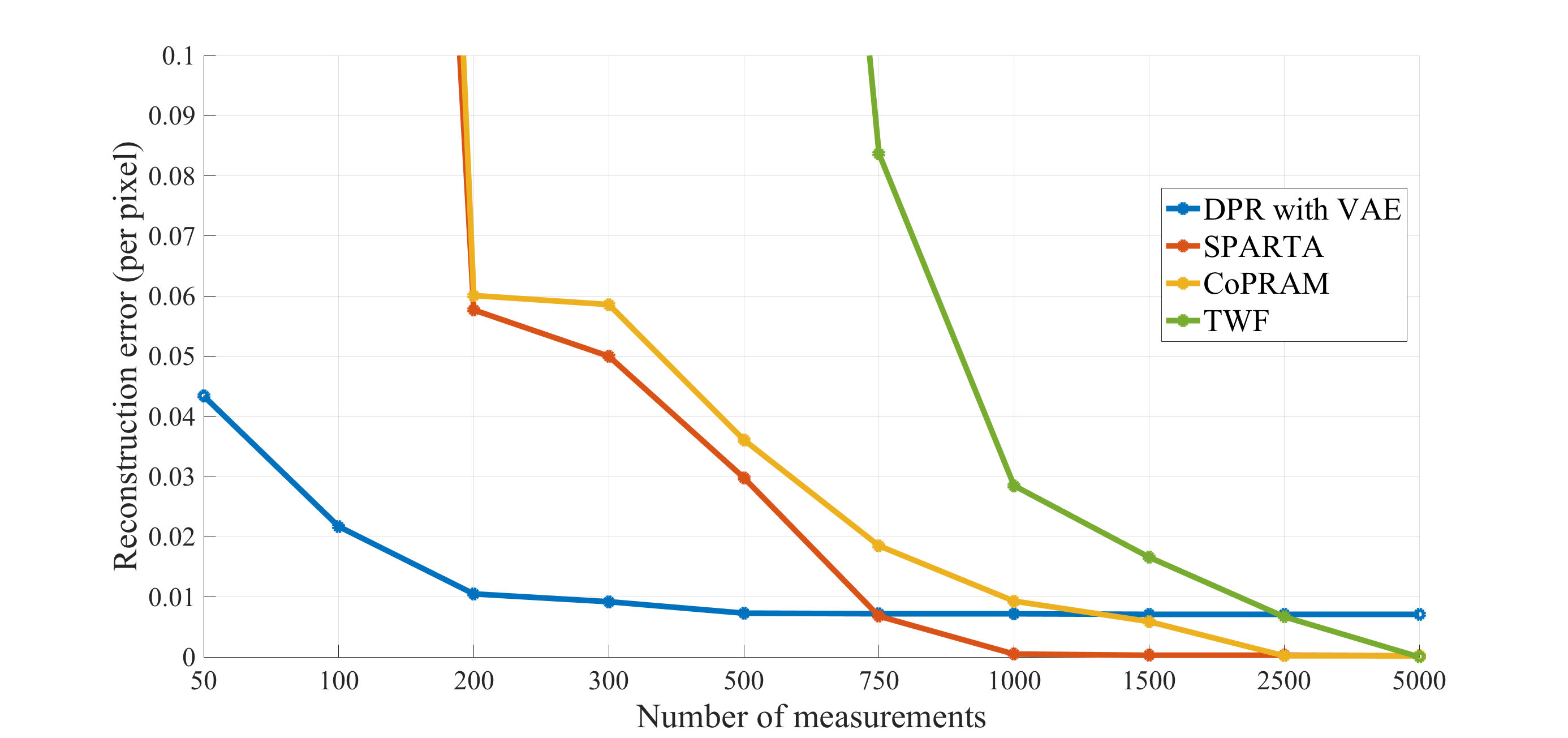
Figure 3: Each algorithm’s average reconstruction error (top) and mean SSIM (bottom) over 1010 images from the MNIST test set for different numbers of measurements.

We attempted to reconstruct 1010 images from the MNIST test set. We allowed 55 random restarts for each algorithm and recorded the result with the least ℓ2\ell_{2} reconstruction error per pixel. In addition, we calculated the Structural Similarity Index Measure (SSIM) [34] for each reconstruction and computed the average for various numbers of measurements. The results in Figure 3 demonstrate the success of our algorithm with very few measurements. For 200200 measurements, we can achieve accurate recovery with a mean SSIM value of over 0.90.9 while other algorithms require 10001000 measurements or more. In terms of reconstruction error, our algorithm exhibits recovery with 200200 measurements comparable to the alternatives requiring 750750 measurements or more, which is where they begin to succeed.

We note that while our algorithm succeeds with fewer measurements than the other methods, our performance, as measured by per-pixel reconstruction error, saturates as the number of measurements increases since our reconstruction accuracy is ultimately bounded by the generative model’s representational error. As generative models improve, their representational errors will decrease. Nonetheless, as can be seen in the reconstructed digits in Figure 4, the recoveries are semantically correct (the correct digit is legibly recovered) even though the reconstruction error does not decay to zero. In applications, such as MRI and molecular structure estimation via X-ray crystallography, semantic error measures would be a more informative estimates of recovery performance than per-pixel error measures.

Refer to caption
Refer to caption
Figure 4: Each algorithm’s reconstructed images with 100100 measurements (left) and 300300 measurements (right). If an image is blank, then the reconstruction error between the blank image and the original image was lower than that of the algorithm’s reconstructed image and the original image. We note that even for as few as 100100 measurements, nearly all of DPR’s reconstructions are semantically correct.

In the second experiment, we used a pretrained Deep Convolutional Generative Adversarial Network (DCGAN) from [4] that was trained on the CelebA dataset [25]. This dataset consists of 200,000200,000 facial images of celebrities. The RGB images were cropped to be of size 64×6464\times 64, resulting in vectorized images of dimension 64×64×3=12288.64\times 64\times 3=12288. The latent code space dimension is k=100k=100. We allowed 22 random restarts. We ran numerical experiments with the other methods and they did not succeed at measurement levels below 50005000. Figure 5 showcases our results in reconstructing 1010 images from the DCGAN’s test set with 500500 measurements. Even for a limited number of measurements, our algorithm’s reconstructions are faithful representations of the original images.

Refer to caption
Figure 5: 1010 reconstructed images from celebA’s test set using DPR with 500500 measurements.

References

  • [1] Sanjeev Arora, Yingyu Liang, and Tengyu Ma. Why are deep nets reversible: A simple theory with implications for training. CoRR, abs/1511.05653, 2015.
  • [2] Sohail Bahmani and Justin Romberg. Efficient compressive phase retrieval with constrained sensing vectors. Advances in Neural Information Processing Systems (NIPS 2015), pages 523–531, 2015.
  • [3] Richard Baraniuk, Mark Davenport, Ronald DeVore, and Michael Wakin. A simple proof of the restricted isometry property for random matrices. Constructive Approximation, 28(3):253–263, 2008.
  • [4] Ashish Bora, Alexandros G. Dimakis, Ajil Jalal, and Eric Price. Compressed sensing using generative models. arXiv preprint arXiv:1703.03208, 2017.
  • [5] Oliver Bunk, Ana Diaz, Franz Pfeiffer, Christian David, Bernd Schmitt, Dillip K. Satapathy, and J. Friso van der Veen. Diffractive imaging for periodic samples: Retrieving one-dimensional concentration profiles across microfluidic channels. Acta Crystallographica Section A: Foundations of Crystallography, 63(4):306–314, 2007.
  • [6] Tony Cai, Xiaodong Li, and Zongming Ma. Optimal rates of convergence for noisy sparse phase retrieval via thresholded wirtinger flow. The Annals of Statistics, 44(5):2221–2251, 2016.
  • [7] Emmanuel J. Candes, Xiaodong Li, and Mahdi Soltanolkotabi. Phase retrieval via wirtinger flow: Theory and applications. IEEE Transactions on Information Theory, 61(4):195–2007, 2017.
  • [8] Emmanuel J. Candes, Thomas Strohmer, and Vladislav Voroninski. Phaselift: Exact and stable signal recovery from magnitude measurements via convex programming. Comm. Pure Applied Math, 66(8):1241–1274, 2013.
  • [9] Yonina C. Eldar, Georgios B. Giannakis, and Gang Wang. Solving systems of random quadratic equations via truncated amplitude flow. IEEE Transactions on Information Theory, 23(26):773–794, 2017.
  • [10] C. Fienup and J. Dainty. Phase retrieval and image reconstruction for astronomy. Image Recovery: Theory and Application, pages 231–275, 1987.
  • [11] J.R. Fienup. Phase retrieval algorithms: A comparison. Applied Optics, 21:2758–2768, 1982.
  • [12] R.W. Gerchberg and W.O. Saxton. A practical algorithm for the determination of phase from image and diffraction plane pictures. Optik, 35:237–246, 1972.
  • [13] Tom Goldstein and Christoph Struder. Phasemax: Convex phase retrieval via basis pursuit. arXiv preprint arXiv: 1610.07531, 2016.
  • [14] Harun Günaydin, Da Tend, Yair Rivenson, Aydogan Ozcan, and Yibo Zhang. Phase recovery and holographic image reconstruction using deep learning in neural networks. arXiv preprint arXiv:1705.04286, 2017.
  • [15] Paul Hand and Vladislav Voroninski. Compressed sensing from phaseless gaussian measurements via linear programming in the natural parameter space. arXiv preprint arXiv:1611.05985, 2016.
  • [16] Paul Hand and Vladislav Voroninski. Global guarantees for enforcing generative priors by empirical risk. arXiv preprint arXiv:1705.07576, 2017.
  • [17] Robert W. Harrison. Phase problem in crystallography. J. Opt. Soc. Am. A, 10(5):1046–1055, 1993.
  • [18] Kishore Jaganathan, Samet Oymak, and Babak Hassibi. Sparse phase retrieval: Convex algorithms and limitations. Information Theory Proceedings (ISIT), 2013 IEEE International Symposium on:1022–1026, 2013.
  • [19] Gauri Jagatap and Chinmay Hegde. Sample-efficient algorithms for recovering structured signals from magnitude-only measurements. Neural Information Processing Systems (NIPS 2017), 2017.
  • [20] Prateek Jain, Praneeth Netrapalli, and Sujay Sanghavi. Phase retrieval using alternating minimization. Neural Information Processing Systems (NIPS 2013), 2013.
  • [21] Diederik Kingma and Jimmy Ba. Adam. Adam: A method for stochastic optimization. arXiv preprint, arXiv:1412.6980, 2014.
  • [22] Yann LeCun, Leon Bottou, Yoshua Bengio, and Patrick Haffner. Gradient-based learning applied to document recognition. Proceedings of the IEEE, 86(11):2278–2324, 1998.
  • [23] Jaehoon Lee, Yasaman Bahri, Roman Novak, Samuel S. Schoenholz, Jeffrey Pennington, and Jascha Sohl-Dickstein. Deep neural networks as gaussian processes. International Conference on Learning Representations (ICLR 2018), 2018.
  • [24] Xiaodong Li and Vladislav Voroninski. Sparse signal recovery from quadratic measurements via convex programming. SIAM Journal on Mathematical Analysis, 45(5):3019–3033, 2013.
  • [25] Ziwei Liu, Ping Luo, Xiaogang Wang, and Xiaoou Tang. Deep learning face attributes in the wild. Proceedings of the IEEE International Conference on Computer Vision, pages 3730–3738, 2015.
  • [26] Jianwei Miao, Tetsuya Ishikawa, Qun Shen, and Thomas Earnest. Extending x-ray crystallography to allow the imaging of noncrystalline materials, cells, and single protein complexes. Annu. Rev. Phys. Chem., 59:387–410, 2008.
  • [27] RP Millane. Phase retrieval in crystallography and optics. J. Opt. Soc. Am. A, 7(3):394–411, 1990.
  • [28] Yaniv Plan and Roman Vershynin. One-bit compressed sensing by linear programming. Communications on Pure and Applied Mathematics, 66(8):1275–1297, 2013.
  • [29] Ju Sun, Qing Qu, and John Wright. A geometric analysis of phase retrieval. Information Theory (ISIT), 2016 IEEE International Symposium, pages 2379–2383, 2016.
  • [30] Roman Vershynin. Introduction to the non-asymptotic analysis of random matrices. Compressed Sensing: Theory and Applications, Cambridge University Press, 2012.
  • [31] Irène Waldspurger, Alexandre d’Aspremont, and Stéphane Mallat. Phase recovery, maxcut and complex semidefinite programming. Mathematical Programming, 149(1-2):47–81, 2015.
  • [32] Adriaan Walther. The question of phase retrieval in optics. Journal of Modern Optics, 10(1):41–49, 1963.
  • [33] Gang Wang, Liang Zhang, Georgios B. Giannakis, Mehmet Akçakaya, and Jie Chen. Sparse phase retrieval via truncated amplitude flow. Signal Processing IEEE Transactions on, 66:479–491, 2018.
  • [34] Zhou Wang, A.C. Bovik, H.R. Sheikh, and E.P. Simoncelli. Image quality assessment: from error visibility to structural similarity. IEEE transactions on image processing, 13(4):600–612, 2004.
  • [35] James G. Wendel. A problem in geometric probability. Math. Scand., 11:109–111, 1962.
  • [36] Li-Hao Yeh, Jonathan Dong, Jingshan Zhong, Lei Tian, Michael Chen, Gongguo Tang, Mahdi Soltanolkotabi, and Laura Waller. Experimental robustness of fourier ptychography phase retrieval algorithms. Optics Express, PP(99):33214–33240, 2015.

5 Appendix

5.1 Full Proof of Theorem 3

Proof.

Set

vx,x0={∇f​(x)f​is differentiable at​x∈ℝklimδ→0+∇f​(x+δ​w)otherwise,\displaystyle v_{x,x_{0}}=\begin{cases}\nabla f(x)\ &\ f\ \text{is differentiable at}\ x\in\mathbb{R}^{k}\\ \lim_{\delta\rightarrow 0^{+}}\nabla f(x+\delta w)\ &\ \text{otherwise,}\end{cases}

where ff is differentiable at x+δ​wx+\delta w for sufficiently small δ>0\delta>0. Recall that

∇f​(x)=(Πi=d1​Wi,+,x)⊤​A⊤​A​(Πi=d1​Wi,+,x)​x−(Πi=d1​Wi,+,x)⊤​AG⁡(x)⊤​AG⁡(x0)​(Πi=d1​Wi,+,x0)​x0.\displaystyle\nabla f(x)=(\Pi_{i=d}^{1}W_{i,+,x})^{\top}A^{\top}A(\Pi_{i=d}^{1}W_{i,+,x})x-(\Pi_{i=d}^{1}W_{i,+,x})^{\top}A_{G(x)}^{\top}A_{G(x_{0})}(\Pi_{i=d}^{1}W_{i,+,x_{0}})x_{0}.

Let

v¯x,x0\displaystyle\overline{v}_{x,x_{0}} :=(Πi=d1​Wi,+,x)⊤​(Πi=d1​Wi,+,x)​x−(Πi=d1​Wi,+,x)⊤​ΦG⁡(x),G⁡(x0)​(Πi=d1​Wi,+,x0)​x0,\displaystyle:=(\Pi_{i=d}^{1}W_{i,+,x})^{\top}(\Pi_{i=d}^{1}W_{i,+,x})x-(\Pi_{i=d}^{1}W_{i,+,x})^{\top}\Phi_{G(x),G(x_{0})}(\Pi_{i=d}^{1}W_{i,+,x_{0}})x_{0}, (5)
hx,x0\displaystyle h_{x,x_{0}} :=−‖x0‖2d​(π−2​θ¯dπ)​(∏i=0d−1π−θ¯iπ)​x^0\displaystyle:=-\frac{\|x_{0}\|}{2^{d}}\left(\frac{\pi-2\overline{\theta}_{d}}{\pi}\right)\left(\prod_{i=0}^{d-1}\frac{\pi-\overline{\theta}_{i}}{\pi}\right)\hat{x}_{0} (6)
+12d​[‖x‖−‖x0‖​(2sinθ¯dπ−(π−2​θ¯dπ)​∑i=0d−1sin⁡θ¯iπ​(∏j=i+1d−1π−θ¯iπ))]​x^,\displaystyle+\frac{1}{2^{d}}\left[\|x\|-\|x_{0}\|\left(\frac{2\sin\overline{\theta}_{d}}{\pi}-\left(\frac{\pi-2\overline{\theta}_{d}}{\pi}\right)\sum_{i=0}^{d-1}\frac{\sin\overline{\theta}_{i}}{\pi}\left(\prod_{j=i+1}^{d-1}\frac{\pi-\overline{\theta}_{i}}{\pi}\right)\right)\right]\hat{x}, (7)

and

Sϵ,x0\displaystyle S_{\epsilon,x_{0}} :={0≠x∈ℝk|‖hx,x0‖≤12d​ϵ​max⁡(‖x‖,‖x0‖)}.\displaystyle:=\left\{0\neq x\in\mathbb{R}^{k}\ |\ \|h_{x,x_{0}}\|\leq\frac{1}{2^{d}}\epsilon\max(\|x\|,\|x_{0}\|)\right\}.

First, observe that by the WDC, we have that for all x≠0x\neq 0 and i=1,…,di=1,\dots,d:

‖Wi,+,x⊤​Wi,+,x−12​Ini‖≤ϵ⟹‖Wi,+,x‖2≤12+ϵ.\displaystyle\left\|W_{i,+,x}^{\top}W_{i,+,x}-\frac{1}{2}I_{n_{i}}\right\|\leq\epsilon\Longrightarrow\|W_{i,+,x}\|^{2}\leq\frac{1}{2}+\epsilon. (8)

Observe that

‖∇f​(x)−v¯x,x0‖\displaystyle\left\|\nabla f(x)-\overline{v}_{x,x_{0}}\right\| ≤‖(Πi=d1​Wi,+,x)⊤​(A⊤​A−Ind)​(Πi=d1​Wi,+,x)​x‖\displaystyle\leq\left\|(\Pi_{i=d}^{1}W_{i,+,x})^{\top}(A^{\top}A-I_{n_{d}})(\Pi_{i=d}^{1}W_{i,+,x})x\right\|
+‖(Πi=d1​Wi,+,x)⊤​(AG⁡(x)⊤​AG⁡(x0)−ΦG⁡(x),G⁡(x0))​(Πi=d1​Wi,+,x0)​x0‖.\displaystyle+\left\|(\Pi_{i=d}^{1}W_{i,+,x})^{\top}(A_{G(x)}^{\top}A_{G(x_{0})}-\Phi_{G(x),G(x_{0})})(\Pi_{i=d}^{1}W_{i,+,x_{0}})x_{0}\right\|.

Hence by the RRCP and (8), we have that

‖∇f​(x)−v¯x,x0‖\displaystyle\left\|\nabla f(x)-\overline{v}_{x,x_{0}}\right\| ≤14​ϵ​(12+ϵ)d​max⁡(‖x‖,‖x0‖).\displaystyle\leq 14\epsilon\left(\frac{1}{2}+\epsilon\right)^{d}\max(\|x\|,\|x_{0}\|). (9)

Then Lemma 2 guarantees that for all non-zero x,x0∈ℝkx,x_{0}\in\mathbb{R}^{k}:

‖v¯x,x0−hx,x0‖≤78​d32d​ϵ​max⁡(‖x‖,‖x0‖).\displaystyle\|\overline{v}_{x,x_{0}}-h_{x,x_{0}}\|\leq 78\frac{d^{3}}{2^{d}}\sqrt{\epsilon}\max(\|x\|,\|x_{0}\|). (10)

Then we have that for all non-zero x,x0∈ℝkx,x_{0}\in\mathbb{R}^{k}:

‖vx,x0−hx,x0‖\displaystyle\|v_{x,x_{0}}-h_{x,x_{0}}\| =limt→0+‖∇f​(x+t​w)−hx+t​w,x0‖\displaystyle=\lim_{t\rightarrow 0^{+}}\|\nabla f(x+tw)-h_{x+tw,x_{0}}\|
≤limt→0+(‖∇f​(x+t​w)−v¯x+t​w,x0‖+‖v¯x+t​w,x0−hx+t​w,x0‖)\displaystyle\leq\lim_{t\rightarrow 0^{+}}\left(\|\nabla f(x+tw)-\overline{v}_{x+tw,x_{0}}\|+\|\overline{v}_{x+tw,x_{0}}-h_{x+tw,x_{0}}\|\right)
≤ϵ​(14​(1+2​ϵ)d2d+78​d32d)​max⁡(‖x‖,‖x0‖)\displaystyle\leq\sqrt{\epsilon}\left(14\frac{(1+2\epsilon)^{d}}{2^{d}}+78\frac{d^{3}}{2^{d}}\right)\max(\|x\|,\|x_{0}\|)
≤ϵ​K​d32d​max⁡(‖x‖,‖x0‖)\displaystyle\leq\sqrt{\epsilon}K\frac{d^{3}}{2^{d}}\max(\|x\|,\|x_{0}\|)

for some universal constant KK where the first equality follows by the definition of vx,x0v_{x,x_{0}} and the continuity of hx,x0h_{x,x_{0}} for non-zero x,x0x,x_{0}. The second inequality combines (9) and (10) and since 2​ϵ​d≤1⟹(1+2​ϵ)d≤e2​ϵ​d≤1+4​ϵ​d.2\epsilon d\leq 1\Longrightarrow(1+2\epsilon)^{d}\leq e^{2\epsilon d}\leq 1+4\epsilon d. This establishes concentration of vx,x0v_{x,x_{0}} to hx,x0h_{x,x_{0}} for all non-zero x,x0∈ℝkx,x_{0}\in\mathbb{R}^{k}:

‖vx,x0−hx,x0‖≤ϵ​K​d32d​max⁡(‖x‖,‖x0‖)\displaystyle\|v_{x,x_{0}}-h_{x,x_{0}}\|\leq\sqrt{\epsilon}K\frac{d^{3}}{2^{d}}\max(\|x\|,\|x_{0}\|) (11)

Now, due to the continuity and piecewise linearity of the function G⁡(x)G(x) and |⋅||\cdot|, we have that for any x,y≠0x,y\neq 0 that there exists a sequence {xn}→x\{x_{n}\}\rightarrow x such that ff is differentiable at each xnx_{n} and Dy​f​(x)=limn→∞∇f​(xn)⋅yD_{y}f(x)=\lim_{n\rightarrow\infty}\nabla f(x_{n})\cdot y. Thus, as ∇f​(xn)=vxn,x0\nabla f(x_{n})=v_{x_{n},x_{0}},

D−vx,x0f(x)=−limn→∞vxn,x0⋅vx,x0.\displaystyle D_{-v_{x,x_{0}}}f(x)=-\lim_{n\rightarrow\infty}v_{x_{n},x_{0}}\cdot v_{x,x_{0}}.

Then observe that

vxn,x0⋅vx,x0\displaystyle v_{x_{n},x_{0}}\cdot v_{x,x_{0}} =hxn,x0⋅hx,x0+(vxn,x0−hxn,x0)⋅hx,x0+hxn,x0⋅(vx,x0−hx,x0)\displaystyle=h_{x_{n},x_{0}}\cdot h_{x,x_{0}}+(v_{x_{n},x_{0}}-h_{x_{n},x_{0}})\cdot h_{x,x_{0}}+h_{x_{n},x_{0}}\cdot(v_{x,x_{0}}-h_{x,x_{0}})
+(vxn,x0−hxn,x0)⋅(vx,x0−hx,x0)\displaystyle+(v_{x_{n},x_{0}}-h_{x_{n},x_{0}})\cdot(v_{x,x_{0}}-h_{x,x_{0}})
≥hxn,x0⋅hx,x0−‖vxn,x0−hxn,x0‖​‖hx,x0‖−‖hxn,x0‖​‖vx,x0−hx,x0‖\displaystyle\geq h_{x_{n},x_{0}}\cdot h_{x,x_{0}}-\|v_{x_{n},x_{0}}-h_{x_{n},x_{0}}\|\|h_{x,x_{0}}\|-\|h_{x_{n},x_{0}}\|\|v_{x,x_{0}}-h_{x,x_{0}}\|
−‖vxn,x0−hxn,x0‖​‖vx,x0−hx,x0‖\displaystyle-\|v_{x_{n},x_{0}}-h_{x_{n},x_{0}}\|\|v_{x,x_{0}}-h_{x,x_{0}}\|
≥hxn,x0⋅hx,x0−‖hx,x0‖​ϵ​K​d32d​max⁡(‖x‖,‖x0‖)\displaystyle\geq h_{x_{n},x_{0}}\cdot h_{x,x_{0}}-\|h_{x,x_{0}}\|\sqrt{\epsilon}K\frac{d^{3}}{2^{d}}\max(\|x\|,\|x_{0}\|)
−|hxn,x0|ϵ​K​d32d​max⁡(‖x‖,‖x0‖)−ϵ​[K​d32d]2​max⁡(‖xn‖,‖x0‖)​max⁡(‖x‖,‖x0‖)\displaystyle-\|h_{x_{n},x_{0}}\|\sqrt{\epsilon}K\frac{d^{3}}{2^{d}}\max(\|x\|,\|x_{0}\|)-\epsilon\left[K\frac{d^{3}}{2^{d}}\right]^{2}\max(\|x_{n}\|,\|x_{0}\|)\max(\|x\|,\|x_{0}\|)

where in the last inequality, we used (11). By the continuity of hx,x0h_{x,x_{0}} for non-zero x∈ℝkx\in\mathbb{R}^{k}, we have that for x∈S4​ϵ​K​d3,x0cx\in S_{4\sqrt{\epsilon}Kd^{3},x_{0}}^{c}:

limn→∞vxn,x0⋅vx,x0\displaystyle\lim_{n\rightarrow\infty}v_{x_{n},x_{0}}\cdot v_{x,x_{0}} ≥‖hx,x0‖2−2​‖hx,x0‖​ϵ​K​d32d​max⁡(‖x‖,‖x0‖)−ϵ​[K​d32d]2​max⁡(‖x‖,‖x0‖)2\displaystyle\geq\|h_{x,x_{0}}\|^{2}-2\|h_{x,x_{0}}\|\sqrt{\epsilon}K\frac{d^{3}}{2^{d}}\max(\|x\|,\|x_{0}\|)-\epsilon\left[K\frac{d^{3}}{2^{d}}\right]^{2}\max(\|x\|,\|x_{0}\|)^{2}
=‖hx,x0‖2​(‖hx,x0‖−4​ϵ​K​d32d​max⁡(‖x‖,‖x0‖))\displaystyle=\frac{\|h_{x,x_{0}}\|}{2}\left(\|h_{x,x_{0}}\|-4\sqrt{\epsilon}K\frac{d^{3}}{2^{d}}\max(\|x\|,\|x_{0}\|)\right)
+12​(‖hx,x0‖2−2​ϵ​[K​d32d]2​max⁡(‖x‖,‖x0‖)2)\displaystyle+\frac{1}{2}\left(\|h_{x,x_{0}}\|^{2}-2\epsilon\left[K\frac{d^{3}}{2^{d}}\right]^{2}\max(\|x\|,\|x_{0}\|)^{2}\right)
>0.\displaystyle>0.

Hence we conclude that for all x∈S4​ϵ​K​d3,x0cx\in S_{4\sqrt{\epsilon}Kd^{3},x_{0}}^{c}, D−vx,x0​f​(x)<0D_{-v_{x,x_{0}}}f(x)<0.

We now show that Dx​f​(0)<0D_{x}f(0)<0 for all x≠0x\neq 0. Note that by direct calculation,

Dxf(0)=−12∑k=1m|⟨ak,(Πi=d1Wi,+,x)x⟩⟨ak,(Πi=d1Wi,+,x0)x0⟩|\displaystyle D_{x}f(0)=-\frac{1}{2}\sum_{k=1}^{m}|\langle a_{k},(\Pi_{i=d}^{1}W_{i,+,x})x\rangle\langle a_{k},(\Pi_{i=d}^{1}W_{i,+,x_{0}})x_{0}\rangle|

where each aka_{k} denotes a row of AA. We further note

|∑k=1m⟨ak,(Πi=d1​Wi,+,x)​x⟩​⟨ak,(Πi=d1​Wi,+,x0)​x0⟩|=|⟨x,(Πi=d1​Wi,+,x)⊤​A⊤​A​(Πi=d1​Wi,+,x0)​x0⟩|\displaystyle\left|\sum_{k=1}^{m}\langle a_{k},(\Pi_{i=d}^{1}W_{i,+,x})x\rangle\langle a_{k},(\Pi_{i=d}^{1}W_{i,+,x_{0}})x_{0}\rangle\right|=\left|\langle x,(\Pi_{i=d}^{1}W_{i,+,x})^{\top}A^{\top}A(\Pi_{i=d}^{1}W_{i,+,x_{0}})x_{0}\rangle\right|

and thus

Dx​f​(0)\displaystyle D_{x}f(0) ≤−12​|⟨x,(Πi=d1​Wi,+,x)⊤​A⊤​A​(Πi=d1​Wi,+,x0)​x0⟩|\displaystyle\leq-\frac{1}{2}\left|\langle x,(\Pi_{i=d}^{1}W_{i,+,x})^{\top}A^{\top}A(\Pi_{i=d}^{1}W_{i,+,x_{0}})x_{0}\rangle\right|
≤−12​⟨x,(Πi=d1​Wi,+,x)⊤​A⊤​A​(Πi=d1​Wi,+,x0)​x0⟩\displaystyle\leq-\frac{1}{2}\langle x,(\Pi_{i=d}^{1}W_{i,+,x})^{\top}A^{\top}A(\Pi_{i=d}^{1}W_{i,+,x_{0}})x_{0}\rangle
=−12​⟨x,(Πi=d1​Wi,+,x)⊤​(A⊤​A−Ind)​(Πi=d1​Wi,+,x0)​x0⟩\displaystyle=-\frac{1}{2}\langle x,(\Pi_{i=d}^{1}W_{i,+,x})^{\top}(A^{\top}A-I_{n_{d}})(\Pi_{i=d}^{1}W_{i,+,x_{0}})x_{0}\rangle
−12​⟨x,(Πi=d1​Wi,+,x)⊤​(Πi=d1​Wi,+,x0)​x0⟩\displaystyle-\frac{1}{2}\langle x,(\Pi_{i=d}^{1}W_{i,+,x})^{\top}(\Pi_{i=d}^{1}W_{i,+,x_{0}})x_{0}\rangle
≤(∗)12​(7​ϵ​(1/2+ϵ)d2d​‖x‖​‖x0‖−14​π​12d​‖x‖​‖x0‖)\displaystyle\stackrel{{\scriptstyle(*)}}{{\leq}}\frac{1}{2}\left(\frac{7\epsilon(1/2+\epsilon)^{d}}{2^{d}}\|x\|\|x_{0}\|-\frac{1}{4\pi}\frac{1}{2^{d}}\|x\|\|x_{0}\|\right)
≤12​(14​ϵ2d​‖x‖​‖x0‖−14​π​12d​‖x‖​‖x0‖)\displaystyle\leq\frac{1}{2}\left(\frac{14\epsilon}{2^{d}}\|x\|\|x_{0}\|-\frac{1}{4\pi}\frac{1}{2^{d}}\|x\|\|x_{0}\|\right)
<0\displaystyle<0

where (∗)(*) follows by the RRCP and Lemma 3 as long as 4​ϵ​d≤14\epsilon d\leq 1 and ϵ<1/(56​π)\epsilon<1/(56\pi).

We conclude by applying Proposition 1 and 24​π​d6​4​ϵ​K​d3≤124\pi d^{6}\sqrt{4\sqrt{\epsilon}Kd^{3}}\leq 1 to attain

S4​ϵ​K​d6⊂ℬ⁡(x0,89​d​4​ϵ​K​d3​‖x0‖)∪ℬ⁡(ρd​x0,836831​d12​4​ϵ​K​d3​‖x0‖).\displaystyle S_{4\sqrt{\epsilon}Kd^{6}}\subset\mathcal{B}(x_{0},89d\sqrt{4\sqrt{\epsilon}Kd^{3}}\|x_{0}\|)\cup\mathcal{B}(\rho_{d}x_{0},836831d^{12}\sqrt{4\sqrt{\epsilon}Kd^{3}}\|x_{0}\|).

∎

We record some results that were used in the above proof. In [16], it was shown that Gaussian WiW_{i} satisfies the WDC with high probability:

Lemma 1 (Lemma 9 in [16]).

Fix 0<ϵ<10<\epsilon<1. Let W∈ℝn×kW\in\mathbb{R}^{n\times k} have i.i.d. 𝒩⁡(0,1/n)\mathcal{N}(0,1/n) entries. If n≥c​k​log⁡kn\geq ck\log k then with probability at least 1−8​n​exp⁡(−γ​k)1-8n\exp(-\gamma k), WW satisfies the WDC with constant ϵ\epsilon. Here c,γ−1c,\gamma^{-1} are constants that depend only polynomially on ϵ−1\epsilon^{-1}.

The following is a technical result showing concentration of v¯x,x0\overline{v}_{x,x_{0}} around hx,x0h_{x,x_{0}}:

Lemma 2.

Fix 0<ϵ<d−4​(1/16​π)20<\epsilon<d^{-4}(1/16\pi)^{2} and let d≥2d\geq 2. Let WiW_{i} satisfy the WDC with constant ϵ\epsilon for i=1,…​di=1,\dots d. For any non-zero x,y∈ℝkx,y\in\mathbb{R}^{k}, we have

‖v¯x,y−hx,y‖≤78​d32d​ϵ​max⁡(‖x‖,‖y‖).\displaystyle\|\overline{v}_{x,y}-h_{x,y}\|\leq\frac{78d^{3}}{2^{d}}\sqrt{\epsilon}\max(\|x\|,\|y\|).
Proof.

Observe that

‖v¯x,y−hx,y‖\displaystyle\|\overline{v}_{x,y}-h_{x,y}\| ≤‖(Πi=d1​Wi,+,x)⊤​(Πi=d1​Wi,+,x)​x−12d​x‖⏟=Q1\displaystyle\leq\underbrace{\left\|(\Pi_{i=d}^{1}W_{i,+,x})^{\top}(\Pi_{i=d}^{1}W_{i,+,x})x-\frac{1}{2^{d}}x\right\|}_{=Q_{1}}\
+‖π−2​θdπ​(Πi=d1​Wi,+,x)⊤​(Πi=d1​Wi,+,y)​y−π−2​θ¯dπ​h~x,y‖⏟=Q2\displaystyle+\underbrace{\left\|\frac{\pi-2\theta_{d}}{\pi}(\Pi_{i=d}^{1}W_{i,+,x})^{\top}(\Pi_{i=d}^{1}W_{i,+,y})y-\frac{\pi-2\overline{\theta}_{d}}{\pi}\tilde{h}_{x,y}\right\|}_{=Q_{2}}\
+‖2sinθdπ​‖(Πi=d1​Wi,+,y)​y‖‖(Πi=d1​Wi,+,x)​x‖​(Πi=d1​Wi,+,x)⊤​(Πi=d1​Wi,+,x)​x−2sinθ¯dπ​‖y‖‖x‖​12d​x‖⏟=Q3.\displaystyle+\underbrace{\left\|\frac{2\sin\theta_{d}}{\pi}\frac{\|(\Pi_{i=d}^{1}W_{i,+,y})y\|}{\|(\Pi_{i=d}^{1}W_{i,+,x})x\|}(\Pi_{i=d}^{1}W_{i,+,x})^{\top}(\Pi_{i=d}^{1}W_{i,+,x})x-\frac{2\sin\overline{\theta}_{d}}{\pi}\frac{\|y\|}{\|x\|}\frac{1}{2^{d}}x\right\|}_{=Q_{3}}.

We focus on bounding each individual quantity QiQ_{i} for i=1,2,3i=1,2,3:

Q1Q_{1}: We have that by (13) in Lemma 3,

‖(Πi=d1​Wi,+,x)⊤​(Πi=d1​Wi,+,x)​x−12d​x‖≤24​d3​ϵ2d​‖x‖.\displaystyle\left\|(\Pi_{i=d}^{1}W_{i,+,x})^{\top}(\Pi_{i=d}^{1}W_{i,+,x})x-\frac{1}{2^{d}}x\right\|\leq 24\frac{d^{3}\sqrt{\epsilon}}{2^{d}}\|x\|. (12)

Q2Q_{2}: We write

Q2\displaystyle Q_{2} ≤‖π−2​θdπ​(Πi=d1​Wi,+,x)⊤​(Πi=d1​Wi,+,y)​y−π−2​θdπ​h~x,y‖\displaystyle\leq\left\|\frac{\pi-2\theta_{d}}{\pi}(\Pi_{i=d}^{1}W_{i,+,x})^{\top}(\Pi_{i=d}^{1}W_{i,+,y})y-\frac{\pi-2\theta_{d}}{\pi}\tilde{h}_{x,y}\right\|
+‖π−2​θdπ​h~x,y−π−2​θ¯dπ​h~x,y‖\displaystyle+\left\|\frac{\pi-2\theta_{d}}{\pi}\tilde{h}_{x,y}-\frac{\pi-2\overline{\theta}_{d}}{\pi}\tilde{h}_{x,y}\right\|
≤(∗)|π−2​θdπ|​24​d3​ϵ2d​‖y‖+|2π​(θd−θ¯d)|​‖h~x,y‖\displaystyle\stackrel{{\scriptstyle(*)}}{{\leq}}\left|\frac{\pi-2\theta_{d}}{\pi}\right|24\frac{d^{3}\sqrt{\epsilon}}{2^{d}}\|y\|+\left|\frac{2}{\pi}(\theta_{d}-\overline{\theta}_{d})\right|\|\tilde{h}_{x,y}\|
≤(∗∗)24​d3​ϵ2d​‖y‖+8​d​ϵπ​(1+dπ)2d​‖y‖\displaystyle\stackrel{{\scriptstyle(**)}}{{\leq}}24\frac{d^{3}\sqrt{\epsilon}}{2^{d}}\|y\|+\frac{8d\sqrt{\epsilon}}{\pi}\frac{\left(1+\frac{d}{\pi}\right)}{2^{d}}\|y\|

where in (∗)(*) we used (13) and (∗∗)(**) used (16) and the fact that ‖h~x,y‖≤2−d​(1+dπ)​‖y‖\|\tilde{h}_{x,y}\|\leq 2^{-d}(1+\frac{d}{\pi})\|y\|. Hence

Q2≤12d​(24​d3+8​dπ​(1+dπ))​ϵ​‖y‖.\displaystyle Q_{2}\leq\frac{1}{2^{d}}\left(24d^{3}+\frac{8d}{\pi}\left(1+\frac{d}{\pi}\right)\right)\sqrt{\epsilon}\|y\|.

Q3Q_{3}: Let yd:=(Πi=d1​Wi,+,y)​yy_{d}:=(\Pi_{i=d}^{1}W_{i,+,y})y and xd:=(Πi=d1​Wi,+,x)​xx_{d}:=(\Pi_{i=d}^{1}W_{i,+,x})x. Then we have that

Q3\displaystyle Q_{3} ≤|2sinθdπ−2sinθ¯dπ|​‖yd‖‖xd‖​‖(Πi=d1​Wi,+,x)⊤​xd‖⏟=Q3,1\displaystyle\leq\underbrace{\left|\frac{2\sin\theta_{d}}{\pi}-\frac{2\sin\overline{\theta}_{d}}{\pi}\right|\frac{\|y_{d}\|}{\|x_{d}\|}\left\|(\Pi_{i=d}^{1}W_{i,+,x})^{\top}x_{d}\right\|}_{=Q_{3,1}}
+‖2sinθ¯dπ​‖yd‖‖xd‖​(Πi=d1​Wi,+,x)⊤​(Πi=d1​Wi,+,x)​x−2sinθ¯dπ​‖y‖‖x‖​(Πi=d1​Wi,+,x)⊤​(Πi=d1​Wi,+,x)​x‖⏟=Q3,2\displaystyle+\underbrace{\left\|\frac{2\sin\overline{\theta}_{d}}{\pi}\frac{\|y_{d}\|}{\|x_{d}\|}(\Pi_{i=d}^{1}W_{i,+,x})^{\top}(\Pi_{i=d}^{1}W_{i,+,x})x-\frac{2\sin\overline{\theta}_{d}}{\pi}\frac{\|y\|}{\|x\|}(\Pi_{i=d}^{1}W_{i,+,x})^{\top}(\Pi_{i=d}^{1}W_{i,+,x})x\right\|}_{=Q_{3,2}}
+‖2sinθ¯dπ​‖y‖‖x‖​(Πi=d1​Wi,+,x)⊤​(Πi=d1​Wi,+,x)​x−2sinθ¯dπ​‖y‖‖x‖​12d​x‖⏟=Q3,3.\displaystyle+\underbrace{\left\|\frac{2\sin\overline{\theta}_{d}}{\pi}\frac{\|y\|}{\|x\|}(\Pi_{i=d}^{1}W_{i,+,x})^{\top}(\Pi_{i=d}^{1}W_{i,+,x})x-\frac{2\sin\overline{\theta}_{d}}{\pi}\frac{\|y\|}{\|x\|}\frac{1}{2^{d}}x\right\|}_{=Q_{3,3}}.

Using (8) and (16) gives

Q3,1\displaystyle Q_{3,1} ≤2π​|θd−θ¯d|​(12+ϵ)d​‖y‖‖x‖​‖x‖\displaystyle\leq\frac{2}{\pi}|\theta_{d}-\overline{\theta}_{d}|\left(\frac{1}{2}+\epsilon\right)^{d}\frac{\|y\|}{\|x\|}\|x\|
≤8​dπ​(12+ϵ)d​ϵ​‖y‖\displaystyle\leq\frac{8d}{\pi}\left(\frac{1}{2}+\epsilon\right)^{d}\sqrt{\epsilon}\|y\|
=8​d​(1+2​ϵ)dπ​2d​ϵ​‖y‖.\displaystyle=\frac{8d(1+2\epsilon)^{d}}{\pi 2^{d}}\sqrt{\epsilon}\|y\|.

Likewise, equations (8) and (15) gives

Q3,2\displaystyle Q_{3,2} ≤|‖yd‖‖xd‖−‖y‖‖x‖|​|2sinθ¯dπ|​(12+ϵ)d​‖x‖\displaystyle\leq\left|\frac{\|y_{d}\|}{\|x_{d}\|}-\frac{\|y\|}{\|x\|}\right|\left|\frac{2\sin\overline{\theta}_{d}}{\pi}\right|\left(\frac{1}{2}+\epsilon\right)^{d}\|x\|
≤8​d​ϵ​‖y‖‖x‖​2π​(12+ϵ)d​‖x‖\displaystyle\leq 8d\epsilon\frac{\|y\|}{\|x\|}\frac{2}{\pi}\left(\frac{1}{2}+\epsilon\right)^{d}\|x\|
≤16​d​ϵπ​(12+ϵ)d​‖y‖\displaystyle\leq\frac{16d\sqrt{\epsilon}}{\pi}\left(\frac{1}{2}+\epsilon\right)^{d}\|y\|
=16​d​(1+2​ϵ)dπ​2d​ϵ​‖y‖\displaystyle=\frac{16d(1+2\epsilon)^{d}}{\pi 2^{d}}\sqrt{\epsilon}\|y\|

Lastly, we use (13) to attain

(3)\displaystyle(3) ≤2π​‖y‖‖x‖​24​d3​ϵ2d​‖x‖\displaystyle\leq\frac{2}{\pi}\frac{\|y\|}{\|x\|}24\frac{d^{3}\sqrt{\epsilon}}{2^{d}}\|x\|
≤48​d3​ϵπ​2d​‖y‖.\displaystyle\leq\frac{48d^{3}\sqrt{\epsilon}}{\pi 2^{d}}\|y\|.

Combining the bounds for Q3,iQ_{3,i} for i=1,2,3i=1,2,3 gives

Q3\displaystyle Q_{3} ≤Q3,1+Q3,2+Q3,3\displaystyle\leq Q_{3,1}+Q_{3,2}+Q_{3,3}
≤8​d​(1+2​ϵ)dπ​2d​ϵ​‖y‖+16​d​(1+2​ϵ)dπ​2d​ϵ​‖y‖+48​d3​ϵπ​2d​‖y‖\displaystyle\leq\frac{8d(1+2\epsilon)^{d}}{\pi 2^{d}}\sqrt{\epsilon}\|y\|+\frac{16d(1+2\epsilon)^{d}}{\pi 2^{d}}\sqrt{\epsilon}\|y\|+\frac{48d^{3}\sqrt{\epsilon}}{\pi 2^{d}}\|y\|
=12d​(24​d​(1+2​ϵ)d+48​d3π)​ϵ​‖y‖.\displaystyle=\frac{1}{2^{d}}\left(\frac{24d(1+2\epsilon)^{d}+48d^{3}}{\pi}\right)\sqrt{\epsilon}\|y\|.

Thus we attain

Q1+Q2+Q3\displaystyle Q_{1}+Q_{2}+Q_{3} ≤Kd2d​ϵ​max⁡(‖x‖,‖y‖)\displaystyle\leq\frac{K_{d}}{2^{d}}\sqrt{\epsilon}\max(\|x\|,\|y\|)

where

Kd\displaystyle K_{d} =24​d3+24​d3+8​d​(1+d/π)π+24​(1+2​ϵ)dπ+48​d3π\displaystyle=24d^{3}+24d^{3}+\frac{8d(1+d/\pi)}{\pi}+\frac{24(1+2\epsilon)^{d}}{\pi}+\frac{48d^{3}}{\pi}
=(48+48π)​d3+8​dπ​(1+dπ+3​d​(1+2​ϵ)d)\displaystyle=\left(48+\frac{48}{\pi}\right)d^{3}+\frac{8d}{\pi}\left(1+\frac{d}{\pi}+3d(1+2\epsilon)^{d}\right)
≤(∗)64​d3+8​dπ​(1+dπ+3​d​(1+4​ϵ​d))\displaystyle\stackrel{{\scriptstyle(*)}}{{\leq}}64d^{3}+\frac{8d}{\pi}\left(1+\frac{d}{\pi}+3d(1+4\epsilon d)\right)
≤64​d3+40​d3+96​ϵ​d3π\displaystyle\leq 64d^{3}+\frac{40d^{3}+96\epsilon d^{3}}{\pi}
≤(∗∗)64​d3+41​d3π\displaystyle\stackrel{{\scriptstyle(**)}}{{\leq}}64d^{3}+\frac{41d^{3}}{\pi}
≤78​d3\displaystyle\leq 78d^{3}

where (∗)(*) and (∗∗)(**) hold as long as ϵ≤min⁡(1/2​d,1/96)\epsilon\leq\min(1/2d,1/96). ∎

The following result summarizes some useful bounds from [16]:

Lemma 3 (Results from Lemma 5 in [16]).

Fix 0<ϵ<d−4​(1/16​π)20<\epsilon<d^{-4}(1/16\pi)^{2} and let d≥2d\geq 2. Let WiW_{i} satisfy the WDC with constant ϵ\epsilon for i=1,…​di=1,\dots d. Then for any non-zero x,y∈ℝkx,y\in\mathbb{R}^{k}, the following hold:

‖(Πi=d1​Wi,+,x)⊤​(Πi=d1​Wi,+,y)​y−h~x,y‖\displaystyle\left\|(\Pi_{i=d}^{1}W_{i,+,x})^{\top}(\Pi_{i=d}^{1}W_{i,+,y})y-\tilde{h}_{x,y}\right\| ≤24​d3​ϵ2d​‖y‖,\displaystyle\leq 24\frac{d^{3}\sqrt{\epsilon}}{2^{d}}\|y\|, (13)
⟨(Πi=d1​Wi,+,x)​x,(Πi=d1​Wi,+,y)​y⟩\displaystyle\left\langle(\Pi_{i=d}^{1}W_{i,+,x})x,(\Pi_{i=d}^{1}W_{i,+,y})y\right\rangle ≥14​π​12d​‖x‖​‖y‖,\displaystyle\geq\frac{1}{4\pi}\frac{1}{2^{d}}\|x\|\|y\|, (14)
|‖yd‖‖xd‖−‖y‖‖x‖|\displaystyle\left|\frac{\|y_{d}\|}{\|x_{d}\|}-\frac{\|y\|}{\|x\|}\right| ≤8​d​ϵ​‖y‖‖x‖,\displaystyle\leq 8d\epsilon\frac{\|y\|}{\|x\|}, (15)
|θd−θ¯d|\displaystyle|\theta_{d}-\overline{\theta}_{d}| ≤4​d​ϵ\displaystyle\leq 4d\sqrt{\epsilon} (16)

where xd:=(Πj=d1​Wj,+x)​xx_{d}:=(\Pi_{j=d}^{1}W_{j,+x})x, yd:=(Πj=d1​Wj,+y)​yy_{d}:=(\Pi_{j=d}^{1}W_{j,+y})y, θd:=∠⁡(xd,yd)\theta_{d}:=\angle(x_{d},y_{d}), θ¯d:=g∘d​(∠⁡(x,y))\overline{\theta}_{d}:=g^{\circ d}(\angle(x,y)), and the vector h~x,y\tilde{h}_{x,y} is defined as

h~x,y:=12d​[(∏i=0d−1π−θ¯iπ)​y+∑i=0d−1sin⁡θ¯iπ​(∏j=i+1d−1π−θ¯iπ)​‖y‖‖x‖​x].\displaystyle\tilde{h}_{x,y}:=\frac{1}{2^{d}}\left[\left(\prod_{i=0}^{d-1}\frac{\pi-\overline{\theta}_{i}}{\pi}\right)y+\sum_{i=0}^{d-1}\frac{\sin\overline{\theta}_{i}}{\pi}\left(\prod_{j=i+1}^{d-1}\frac{\pi-\overline{\theta}_{i}}{\pi}\right)\frac{\|y\|}{\|x\|}x\right].

.

5.2 Determining where hx,x0h_{x,x_{0}} vanishes

Before proving Proposition 1, we outline how the vector hx,x0h_{x,x_{0}} was derived. Recall that

∇f​(x)=(Πi=d1​Wi,+,x)⊤​A⊤​A​(Πi=d1​Wi,+,x)​x−(Πi=d1​Wi,+,x)⊤​AG⁡(x)⊤​AG⁡(x0)​(Πi=d1​Wi,+,x0)​x0.\displaystyle\nabla f(x)=(\Pi_{i=d}^{1}W_{i,+,x})^{\top}A^{\top}A(\Pi_{i=d}^{1}W_{i,+,x})x-(\Pi_{i=d}^{1}W_{i,+,x})^{\top}A_{G(x)}^{\top}A_{G(x_{0})}(\Pi_{i=d}^{1}W_{i,+,x_{0}})x_{0}.

The concentration of the first term follows by the RRCP and Lemma 3:

(Πi=d1​Wi,+,x)⊤​A⊤​A​(Πi=d1​Wi,+,x)​x≈(Πi=d1​Wi,+,x)⊤​(Πi=d1​Wi,+,x)​x≈h~x,x=12d​x.\displaystyle(\Pi_{i=d}^{1}W_{i,+,x})^{\top}A^{\top}A(\Pi_{i=d}^{1}W_{i,+,x})x\approx(\Pi_{i=d}^{1}W_{i,+,x})^{\top}(\Pi_{i=d}^{1}W_{i,+,x})x\approx\tilde{h}_{x,x}=\frac{1}{2^{d}}x.

For the second term, note that the RRCP gives

(Πi=d1​Wi,+,x)⊤​AG⁡(x)⊤​AG⁡(x0)​(Πi=d1​Wi,+,x0)​x0≈(Πi=d1​Wi,+,x)⊤​ΦG⁡(x),G⁡(x0)​(Πi=d1​Wi,+,x0)​x0.\displaystyle(\Pi_{i=d}^{1}W_{i,+,x})^{\top}A_{G(x)}^{\top}A_{G(x_{0})}(\Pi_{i=d}^{1}W_{i,+,x_{0}})x_{0}\approx(\Pi_{i=d}^{1}W_{i,+,x})^{\top}\Phi_{G(x),G(x_{0})}(\Pi_{i=d}^{1}W_{i,+,x_{0}})x_{0}.

Letting xd=(Πi=d1​Wi,+,x)​x=G⁡(x)x_{d}=(\Pi_{i=d}^{1}W_{i,+,x})x=G(x) and x0,d=(Πi=d1​Wi,+,x0)​x0=G⁡(x0)x_{0,d}=(\Pi_{i=d}^{1}W_{i,+,x_{0}})x_{0}=G(x_{0}), note that

Φxd,x0,d=π−2​θdπ​I+2sinθdπ​Mx^d↔x^0,d\displaystyle\Phi_{x_{d},x_{0,d}}=\frac{\pi-2\theta_{d}}{\pi}I+\frac{2\sin\theta_{d}}{\pi}M_{\hat{x}_{d}\leftrightarrow\hat{x}_{0,d}}

where θd=∠⁡(xd,x0,d)\theta_{d}=\angle(x_{d},x_{0,d}). By Lemma 5 in [16], this angle is well-defined and ‖xd‖,‖x0,d‖≠0\|x_{d}\|,\|x_{0,d}\|\neq 0 as long as each WiW_{i} satisfies the WDC. Finally, note that the definition of Mx^↔y^M_{\hat{x}\leftrightarrow\hat{y}} gives

Mx^d↔x^0,d​x0,d\displaystyle M_{\hat{x}_{d}\leftrightarrow\hat{x}_{0,d}}x_{0,d} =‖x0,d‖​Mx^d↔x^0,d​x^0,d=‖x0,d‖​x^d=‖x0,d‖‖xd‖​xd.\displaystyle=\|x_{0,d}\|M_{\hat{x}_{d}\leftrightarrow\hat{x}_{0,d}}\hat{x}_{0,d}=\|x_{0,d}\|\hat{x}_{d}=\frac{\|x_{0,d}\|}{\|x_{d}\|}x_{d}.

Thus we see that

(Πi=d1​Wi,+,x)⊤​Φxd,x0,d​(Πi=d1​Wi,+,x0)​x0\displaystyle(\Pi_{i=d}^{1}W_{i,+,x})^{\top}\Phi_{x_{d},x_{0,d}}(\Pi_{i=d}^{1}W_{i,+,x_{0}})x_{0}
=π−2​θdπ​(Πi=d1​Wi,+,x)⊤​(Πi=d1​Wi,+,x0)​x0+2sinθdπ​‖x0,d‖‖xd‖​(Πi=d1​Wi,+,x)⊤​(Πi=d1​Wi,+,x)​x\displaystyle=\frac{\pi-2\theta_{d}}{\pi}(\Pi_{i=d}^{1}W_{i,+,x})^{\top}(\Pi_{i=d}^{1}W_{i,+,x_{0}})x_{0}+\frac{2\sin\theta_{d}}{\pi}\frac{\|x_{0,d}\|}{\|x_{d}\|}(\Pi_{i=d}^{1}W_{i,+,x})^{\top}(\Pi_{i=d}^{1}W_{i,+,x})x
≈π−2​θ¯dπ​h~x,x0+2sinθ¯dπ​‖x0‖‖x‖​12d​x\displaystyle\approx\frac{\pi-2\overline{\theta}_{d}}{\pi}\tilde{h}_{x,x_{0}}+\frac{2\sin\overline{\theta}_{d}}{\pi}\frac{\|x_{0}\|}{\|x\|}\frac{1}{2^{d}}x

where θ¯d=g∘d​(∠⁡(x,x0))\overline{\theta}_{d}=g^{\circ d}(\angle(x,x_{0})) and the definition of h~x,x0\tilde{h}_{x,x_{0}} is given in Lemma 3. The concentration of the angle θd\theta_{d} and norm ‖x0,d‖/‖xd‖\|x_{0,d}\|/\|x_{d}\| are given in Lemma 3. Combining the concentrations of the two terms in ∇f​(x)\nabla f(x) gives hx,x0h_{x,x_{0}}.

Now, we establish that the set of all xx such that ‖hx,x0‖≈0\|h_{x,x_{0}}\|\approx 0, denoted by Sϵ,x0S_{\epsilon,x_{0}}, is contained in two neighborhoods centered at x0x_{0} and a negative multiple −ρd​x0-\rho_{d}x_{0}.

Proposition 1.

Suppose 24​π​d6​ϵ≤1.24\pi d^{6}\sqrt{\epsilon}\leq 1. Let

Sϵ,x0={0≠x∈ℝk|‖hx,x0‖≤12d​ϵ​max⁡(‖x‖,‖x0‖)}\displaystyle S_{\epsilon,x_{0}}=\left\{0\neq x\in\mathbb{R}^{k}\ |\ \|h_{x,x_{0}}\|\leq\frac{1}{2^{d}}\epsilon\max(\|x\|,\|x_{0}\|)\right\}

where d≥2d\geq 2 and let

hx,x0\displaystyle h_{x,x_{0}} =−‖x0‖2d​(π−2​θ¯dπ)​(∏i=0d−1π−θ¯iπ)​x^0\displaystyle=-\frac{\|x_{0}\|}{2^{d}}\left(\frac{\pi-2\overline{\theta}_{d}}{\pi}\right)\left(\prod_{i=0}^{d-1}\frac{\pi-\overline{\theta}_{i}}{\pi}\right)\hat{x}_{0}
+12d​[‖x‖−‖x0‖​(2sinθ¯dπ−(π−2​θ¯dπ)​∑i=0d−1sin⁡θ¯iπ​(∏j=i+1d−1π−θ¯iπ))]​x^.\displaystyle+\frac{1}{2^{d}}\left[\|x\|-\|x_{0}\|\left(\frac{2\sin\overline{\theta}_{d}}{\pi}-\left(\frac{\pi-2\overline{\theta}_{d}}{\pi}\right)\sum_{i=0}^{d-1}\frac{\sin\overline{\theta}_{i}}{\pi}\left(\prod_{j=i+1}^{d-1}\frac{\pi-\overline{\theta}_{i}}{\pi}\right)\right)\right]\hat{x}.

where θ¯0=∠⁡(x,x0)\overline{\theta}_{0}=\angle(x,x_{0}) and θ¯i=g⁡(θ¯i−1)\overline{\theta}_{i}=g(\overline{\theta}_{i-1}). Define

ρd:=−2sinθ˘dπ+(π−2​θ˘dπ)​∑i=0d−1sin⁡θ˘iπ​(∏j=i+1d−1π−θ˘iπ)\displaystyle\rho_{d}:=-\frac{2\sin\breve{\theta}_{d}}{\pi}+\left(\frac{\pi-2\breve{\theta}_{d}}{\pi}\right)\sum_{i=0}^{d-1}\frac{\sin\breve{\theta}_{i}}{\pi}\left(\prod_{j=i+1}^{d-1}\frac{\pi-\breve{\theta}_{i}}{\pi}\right)

where θ˘0=π\breve{\theta}_{0}=\pi and θ˘i=g⁡(θ˘i−1)\breve{\theta}_{i}=g(\breve{\theta}_{i-1}). If x∈Sϵ,x0x\in S_{\epsilon,x_{0}}, then either

|θ¯0|≤2​ϵ​and​|‖x‖−‖x0‖|≤29​d​ϵ​‖x0‖\displaystyle|\overline{\theta}_{0}|\leq 2\sqrt{\epsilon}\ \text{and}\ |\|x\|-\|x_{0}\||\leq 29d\sqrt{\epsilon}\|x_{0}\|

or

|θ¯0−π|≤24​π2​d4​ϵ​and​|‖x‖−ρd​‖x0‖|≤3517​d8​ϵ​‖x0‖.\displaystyle|\overline{\theta}_{0}-\pi|\leq 24\pi^{2}d^{4}\sqrt{\epsilon}\ \text{and}\ |\|x\|-\rho_{d}\|x_{0}\||\leq 3517d^{8}\sqrt{\epsilon}\|x_{0}\|.

In particular, we have

Sϵ,x0⊂ℬ⁡(x0,89​d​ϵ​‖x0‖)∪ℬ⁡(−ρd​x0,836831​d12​ϵ​‖x0‖).\displaystyle S_{\epsilon,x_{0}}\subset\mathcal{B}(x_{0},89d\sqrt{\epsilon}\|x_{0}\|)\cup\mathcal{B}(-\rho_{d}x_{0},836831d^{12}\sqrt{\epsilon}\|x_{0}\|).

Additionally, ρd→1\rho_{d}\rightarrow 1 as d→∞d\rightarrow\infty.

Proof.

Without loss of generality, let x0=e1x_{0}=e_{1} and ‖x0‖=1\|x_{0}\|=1 where e1e_{1} is the first standard basis vector in ℝk\mathbb{R}^{k}. We also set x=|x|(cos⁡θ¯0​e1+sin⁡θ¯0​e2)x=\|x\|\left(\cos\overline{\theta}_{0}e_{1}+\sin\overline{\theta}_{0}e_{2}\right) where θ¯0=∠⁡(x,x0)\overline{\theta}_{0}=\angle(x,x_{0}). Then

hx,x0\displaystyle h_{x,x_{0}} =−12d​(π−2​θ¯dπ)​(∏i=0d−1π−θ¯iπ)​x^0\displaystyle=-\frac{1}{2^{d}}\left(\frac{\pi-2\overline{\theta}_{d}}{\pi}\right)\left(\prod_{i=0}^{d-1}\frac{\pi-\overline{\theta}_{i}}{\pi}\right)\hat{x}_{0}
+12d​[‖x‖−(2sinθ¯dπ−(π−2​θ¯dπ)​∑i=0d−1sin⁡θ¯iπ​(∏j=i+1d−1π−θ¯iπ))]​x^.\displaystyle+\frac{1}{2^{d}}\left[\|x\|-\left(\frac{2\sin\overline{\theta}_{d}}{\pi}-\left(\frac{\pi-2\overline{\theta}_{d}}{\pi}\right)\sum_{i=0}^{d-1}\frac{\sin\overline{\theta}_{i}}{\pi}\left(\prod_{j=i+1}^{d-1}\frac{\pi-\overline{\theta}_{i}}{\pi}\right)\right)\right]\hat{x}.

Set

β=(π−2​θ¯dπ)​(∏i=0d−1π−θ¯iπ)​and​α=2sinθ¯dπ−(π−2​θ¯dπ)​∑i=0d−1sin⁡θ¯iπ​(∏j=i+1d−1π−θ¯iπ)\displaystyle\beta=\left(\frac{\pi-2\overline{\theta}_{d}}{\pi}\right)\left(\prod_{i=0}^{d-1}\frac{\pi-\overline{\theta}_{i}}{\pi}\right)\ \text{and}\ \alpha=\frac{2\sin\overline{\theta}_{d}}{\pi}-\left(\frac{\pi-2\overline{\theta}_{d}}{\pi}\right)\sum_{i=0}^{d-1}\frac{\sin\overline{\theta}_{i}}{\pi}\left(\prod_{j=i+1}^{d-1}\frac{\pi-\overline{\theta}_{i}}{\pi}\right)

with r=‖x‖r=\|x\| and M=max⁡(r,1)M=\max(r,1). Note that we can write

hx,x0=12d​(−β​x^0+(r−α)​x^)\displaystyle h_{x,x_{0}}=\frac{1}{2^{d}}\left(-\beta\hat{x}_{0}+(r-\alpha)\hat{x}\right)

Then if x∈Sϵ,x0x\in S_{\epsilon,x_{0}}, we have that

|−β+cos⁡θ¯0​(r−α)|\displaystyle|-\beta+\cos\overline{\theta}_{0}(r-\alpha)| ≤ϵ​M\displaystyle\leq\epsilon M (17)
|sin⁡θ¯0​(r−α)|\displaystyle|\sin\overline{\theta}_{0}(r-\alpha)| ≤ϵ​M.\displaystyle\leq\epsilon M. (18)

We now tabulate some useful bounds from Lemma 8 in [16]:

θ¯i\displaystyle\overline{\theta}_{i} ∈[0,π/2]​for​i≥1\displaystyle\in[0,\pi/2]\ \text{for}\ i\geq 1 (19)
θ¯i\displaystyle\overline{\theta}_{i} ≤θ¯i−1​for​i≥1\displaystyle\leq\overline{\theta}_{i-1}\ \text{for}\ i\geq 1 (20)
|∏i=0d−1π−θ¯iπ|\displaystyle\left|\prod_{i=0}^{d-1}\frac{\pi-\overline{\theta}_{i}}{\pi}\right| ≤1\displaystyle\leq 1 (21)
∏i=0d−1π−θ¯iπ\displaystyle\prod_{i=0}^{d-1}\frac{\pi-\overline{\theta}_{i}}{\pi} ≥π−θ¯0π​d3\displaystyle\geq\frac{\pi-\overline{\theta}_{0}}{\pi d^{3}} (22)
|∑i=0d−1sin⁡θ¯iπ​(∏j=i+1d−1π−θ¯iπ)|\displaystyle\left|\sum_{i=0}^{d-1}\frac{\sin\overline{\theta}_{i}}{\pi}\left(\prod_{j=i+1}^{d-1}\frac{\pi-\overline{\theta}_{i}}{\pi}\right)\right| ≤dπsinθ¯0\displaystyle\leq\frac{d}{\pi}\sin\overline{\theta}_{0} (23)
θ¯0=π+O1​(δ)\displaystyle\overline{\theta}_{0}=\pi+O_{1}(\delta) ⟹θ¯i=θ˘i+O1​(i​δ)\displaystyle\Longrightarrow\overline{\theta}_{i}=\breve{\theta}_{i}+O_{1}(i\delta) (24)
θ¯0=π+O1​(δ)\displaystyle\overline{\theta}_{0}=\pi+O_{1}(\delta) ⟹|∏i=0d−1π−θ¯iπ|≤δπ\displaystyle\Longrightarrow\left|\prod_{i=0}^{d-1}\frac{\pi-\overline{\theta}_{i}}{\pi}\right|\leq\frac{\delta}{\pi} (25)
|π−2​θ¯iπ|\displaystyle\left|\frac{\pi-2\overline{\theta}_{i}}{\pi}\right| ≤1​∀i≥1\displaystyle\leq 1\ \forall\ i\geq 1 (26)
θ¯d\displaystyle\overline{\theta}_{d} ≤cos−1⁡(1π)​∀d≥2.\displaystyle\leq\cos^{-1}\left(\frac{1}{\pi}\right)\ \forall\ d\geq 2. (27)

To prove the Proposition, we first show that it is sufficient to only consider the small and large angle case. Then, we show that in the small and large angle case, x≈x0x\approx x_{0} and x≈−ρd​x0x\approx-\rho_{d}x_{0}, respectively. We begin by proving that max⁡(‖x‖,‖x0‖)≤6​d\max(\|x\|,\|x_{0}\|)\leq 6d for any x∈Sϵ,x0x\in S_{\epsilon,x_{0}}.

Bound on maximal norm in Sϵ,x0S_{\epsilon,x_{0}}: It suffices to show that r≤6​dr\leq 6d. Suppose r>1r>1 since if r≤1r\leq 1, the result is immediate. Then either |sin⁡θ¯0|≥1/2|\sin\overline{\theta}_{0}|\geq 1/\sqrt{2} or |cos⁡θ¯0|≥1/2|\cos\overline{\theta}_{0}|\geq 1/\sqrt{2}. If |sin⁡θ¯0|≥1/2|\sin\overline{\theta}_{0}|\geq 1/\sqrt{2} then (18) gives

|r−α|≤2​ϵ​r⟹(1−2​ϵ)​r≤|α|.\displaystyle|r-\alpha|\leq\sqrt{2}\epsilon r\Longrightarrow(1-\sqrt{2}\epsilon)r\leq|\alpha|.

But

|α|\displaystyle|\alpha| ≤2π​|sin⁡θ¯d|+|(π−2​θ¯dπ)​∑i=0d−1sin⁡θ¯iπ​(∏j=i+1d−1π−θ¯iπ)|\displaystyle\leq\frac{2}{\pi}|\sin\overline{\theta}_{d}|+\left|\left(\frac{\pi-2\overline{\theta}_{d}}{\pi}\right)\sum_{i=0}^{d-1}\frac{\sin\overline{\theta}_{i}}{\pi}\left(\prod_{j=i+1}^{d-1}\frac{\pi-\overline{\theta}_{i}}{\pi}\right)\right|
≤1+dπ\displaystyle\leq 1+\frac{d}{\pi}

where the second inequality used equations (23) and (26). Thus

r≤1+dπ1−2​ϵ≤2​(1+dπ)≤2+d≤2​d\displaystyle r\leq\frac{1+\frac{d}{\pi}}{1-\sqrt{2}\epsilon}\leq 2\left(1+\frac{d}{\pi}\right)\leq 2+d\leq 2d

provided ϵ<1/4\epsilon<1/4 and d≥2d\geq 2. If |cos⁡θ¯0|≥1/2|\cos\overline{\theta}_{0}|\geq 1/\sqrt{2}, then (17) gives

|r−α|≤2​(ϵ​r+|β|)⟹(1−2​ϵ)​r≤2​|β|+α.\displaystyle|r-\alpha|\leq\sqrt{2}(\epsilon r+|\beta|)\Longrightarrow(1-\sqrt{2}\epsilon)r\leq\sqrt{2}|\beta|+\alpha.

But by (21),

|β|=|(π−2​θ¯dπ)​(∏i=0d−1π−θ¯iπ)|≤1​since​θ¯i∈[0,π/2]​∀i≥1.\displaystyle|\beta|=\left|\left(\frac{\pi-2\overline{\theta}_{d}}{\pi}\right)\left(\prod_{i=0}^{d-1}\frac{\pi-\overline{\theta}_{i}}{\pi}\right)\right|\leq 1\ \text{since}\ \overline{\theta}_{i}\in[0,\pi/2]\ \forall\ i\ \geq 1.

Hence if ϵ<1/4\epsilon<1/4,

r≤2+2​d1−2​ϵ≤2​2+4​d≤2​d+4​d≤6​d.\displaystyle r\leq\frac{\sqrt{2}+2d}{1-\sqrt{2}\epsilon}\leq 2\sqrt{2}+4d\leq\sqrt{2}d+4d\leq 6d.

Thus in any case, r≤6​d⟹M≤6​dr\leq 6d\Longrightarrow M\leq 6d.

We now show that it is sufficient to only consider the small angle case θ¯0≈0\overline{\theta}_{0}\approx 0 and the large angle case θ¯0≈π\overline{\theta}_{0}\approx\pi.

Sufficiency: We have two possible situations:

  • •

    |r−α|≥ϵ​M|r-\alpha|\geq\sqrt{\epsilon}M: Then (18) implies

    |sin⁡θ¯0|≤ϵ⟹θ¯0=O1​(2​ϵ)​or​π+O1​(2​ϵ).\displaystyle|\sin\overline{\theta}_{0}|\leq\sqrt{\epsilon}\Longrightarrow\overline{\theta}_{0}=O_{1}(2\sqrt{\epsilon})\ \text{or}\ \pi+O_{1}(2\sqrt{\epsilon}).
  • •

    |r−α|≤ϵ​M:|r-\alpha|\leq\sqrt{\epsilon}M: Then (17) implies

    |β|≤2​ϵ​M.\displaystyle|\beta|\leq 2\sqrt{\epsilon}M.

    But note that by (22),

    β=(π−2​θ¯dπ)​(∏i=0d−1π−θ¯iπ)≥(π−2​θ¯d)​(π−θ¯0)d3​π2.\displaystyle\beta=\left(\frac{\pi-2\overline{\theta}_{d}}{\pi}\right)\left(\prod_{i=0}^{d-1}\frac{\pi-\overline{\theta}_{i}}{\pi}\right)\geq\frac{(\pi-2\overline{\theta}_{d})(\pi-\overline{\theta}_{0})}{d^{3}\pi^{2}}.

    In addition, (27) implies

    |π−2​θ¯d|≥|π−2​cos−1⁡(1π)|≥12.\displaystyle|\pi-2\overline{\theta}_{d}|\geq\left|\pi-2\cos^{-1}\left(\frac{1}{\pi}\right)\right|\geq\frac{1}{2}.

    Thus

    |β|≥|(π−2​θ¯d)​(π−θ¯0)|d3​π2≥|π−θ¯0|2​d3​π2\displaystyle|\beta|\geq\frac{|(\pi-2\overline{\theta}_{d})(\pi-\overline{\theta}_{0})|}{d^{3}\pi^{2}}\geq\frac{|\pi-\overline{\theta}_{0}|}{2d^{3}\pi^{2}}

    which implies

    |π−θ¯0|≤4​d3​π2​ϵ​M≤24​d4​π2​ϵ.\displaystyle|\pi-\overline{\theta}_{0}|\leq 4d^{3}\pi^{2}\sqrt{\epsilon}M\leq 24d^{4}\pi^{2}\sqrt{\epsilon}.

    Thus θ¯0=π+O1​(24​d4​π2​ϵ)\overline{\theta}_{0}=\pi+O_{1}(24d^{4}\pi^{2}\sqrt{\epsilon}).

Lastly, we show that in the small angle case, x≈x0x\approx x_{0}, while in the large angle case, x≈−ρd​x0x\approx-\rho_{d}x_{0}.

Small Angle Case: Assume θ¯0=O1​(2​ϵ)\overline{\theta}_{0}=O_{1}(2\sqrt{\epsilon}). Note that since θ¯i≤θ¯0≤2​ϵ\overline{\theta}_{i}\leq\overline{\theta}_{0}\leq 2\sqrt{\epsilon} for each ii, we have that

∏i=0d−1π−θ¯iπ≥(1−2​ϵπ)d=1+O1​(4​d​ϵπ)\displaystyle\prod_{i=0}^{d-1}\frac{\pi-\overline{\theta}_{i}}{\pi}\geq\left(1-\frac{2\sqrt{\epsilon}}{\pi}\right)^{d}=1+O_{1}\left(\frac{4d\sqrt{\epsilon}}{\pi}\right)

provided 2​d​ϵ≤1/22d\sqrt{\epsilon}\leq 1/2. Hence

β\displaystyle\beta =(π−2​θ¯dπ)​(∏i=0d−1π−θ¯iπ)\displaystyle=\left(\frac{\pi-2\overline{\theta}_{d}}{\pi}\right)\left(\prod_{i=0}^{d-1}\frac{\pi-\overline{\theta}_{i}}{\pi}\right)
≥(1+O1​(4​ϵπ))​(1+O1​(4​d​ϵπ))\displaystyle\geq\left(1+O_{1}\left(\frac{4\sqrt{\epsilon}}{\pi}\right)\right)\left(1+O_{1}\left(\frac{4d\sqrt{\epsilon}}{\pi}\right)\right)\

where we used (24) in the second inequality. In addition, |sin⁡θ¯d|≤|θ¯d|≤2​ϵ|\sin\overline{\theta}_{d}|\leq|\overline{\theta}_{d}|\leq 2\sqrt{\epsilon} and (23) imply that

|∑i=0d−1sin⁡θ¯iπ​(∏j=i+1d−1π−θ¯iπ)|≤dπ​|sin⁡θ¯d|≤d​ϵ.\displaystyle\left|\sum_{i=0}^{d-1}\frac{\sin\overline{\theta}_{i}}{\pi}\left(\prod_{j=i+1}^{d-1}\frac{\pi-\overline{\theta}_{i}}{\pi}\right)\right|\leq\frac{d}{\pi}|\sin\overline{\theta}_{d}|\leq d\sqrt{\epsilon}.

Hence

α\displaystyle\alpha =2sinθ¯dπ−(π−2​θ¯dπ)​∑i=0d−1sin⁡θ¯iπ​(∏j=i+1d−1π−θ¯iπ)\displaystyle=\frac{2\sin\overline{\theta}_{d}}{\pi}-\left(\frac{\pi-2\overline{\theta}_{d}}{\pi}\right)\sum_{i=0}^{d-1}\frac{\sin\overline{\theta}_{i}}{\pi}\left(\prod_{j=i+1}^{d-1}\frac{\pi-\overline{\theta}_{i}}{\pi}\right)
=O1​(4​ϵ3​π)+(1+O1​(4​ϵπ))​O1​(d​ϵ)\displaystyle=O_{1}\left(\frac{4\sqrt{\epsilon}}{3\pi}\right)+\left(1+O_{1}\left(\frac{4\sqrt{\epsilon}}{\pi}\right)\right)O_{1}(d\sqrt{\epsilon})
=O1​(4​ϵ3​π)+O1​(d​ϵ)+O1​(4​d​ϵπ)\displaystyle=O_{1}\left(\frac{4\sqrt{\epsilon}}{3\pi}\right)+O_{1}(d\sqrt{\epsilon})+O_{1}\left(\frac{4d\epsilon}{\pi}\right)
=O1​((4+3​d​π+12​d)​ϵ3​π)\displaystyle=O_{1}\left(\frac{(4+3d\pi+12d)\sqrt{\epsilon}}{3\pi}\right)

Thus since |−β+cos⁡θ¯0​(r−α)|≤ϵ​M|-\beta+\cos\overline{\theta}_{0}(r-\alpha)|\leq\epsilon M and M≤6​dM\leq 6d, we attain

−(1+O1​(4​ϵπ))​(1+O1​(4​d​ϵπ))\displaystyle-\left(1+O_{1}\left(\frac{4\sqrt{\epsilon}}{\pi}\right)\right)\left(1+O_{1}\left(\frac{4d\sqrt{\epsilon}}{\pi}\right)\right) +(1+O1​(2​ϵ))​(r+O1​((4+3​d​π+12​d)​ϵ3​π))\displaystyle+(1+O_{1}(2\epsilon))\left(r+O_{1}\left(\frac{(4+3d\pi+12d)\sqrt{\epsilon}}{3\pi}\right)\right)
=O1​(6​d​ϵ).\displaystyle=O_{1}(6d\epsilon).

Rearranging, this gives

r−1\displaystyle r-1 =O1​(4​d​ϵπ+4​ϵπ+16​d​ϵπ+(2​ϵ+1)​(4+3​d​π+12​d)​ϵ3​π)+O1​(12​d​ϵ)+O1​(6​d​ϵ)\displaystyle=O_{1}\left(\frac{4d\sqrt{\epsilon}}{\pi}+\frac{4\sqrt{\epsilon}}{\pi}+\frac{16d\epsilon}{\pi}+(2\epsilon+1)\frac{(4+3d\pi+12d)\sqrt{\epsilon}}{3\pi}\right)+O_{1}(12d\epsilon)+O_{1}(6d\epsilon)
=O1​((12​d+12+48​d)​ϵ+(2​ϵ+1)​(4+3​π​d+12​d)​ϵ3​π+18​d​ϵ)\displaystyle=O_{1}\left(\frac{(12d+12+48d)\sqrt{\epsilon}+(2\epsilon+1)(4+3\pi d+12d)\sqrt{\epsilon}}{3\pi}+18d\sqrt{\epsilon}\right)
=O1​(29​d​ϵ).\displaystyle=O_{1}(29d\sqrt{\epsilon}).

Large Angle Case: Assume θ¯0=π+O1​(δ)\overline{\theta}_{0}=\pi+O_{1}(\delta) where δ:=24​d4​π2​ϵ.\delta:=24d^{4}\pi^{2}\sqrt{\epsilon}. We first prove that α\alpha is close to ρd\rho_{d} in the O1O_{1} sense. Recall that θ¯d=θ˘d+O1​(d​δ)\overline{\theta}_{d}=\breve{\theta}_{d}+O_{1}(d\delta). Then by the mean value theorem:

|sin⁡θ¯d−sin⁡θ˘d|≤|θ¯d−θ˘d|≤d​δ\displaystyle|\sin\overline{\theta}_{d}-\sin\breve{\theta}_{d}|\leq|\overline{\theta}_{d}-\breve{\theta}_{d}|\leq d\delta

so sin⁡θ¯d=sin⁡θ˘d+O1​(d​δ)\sin\overline{\theta}_{d}=\sin\breve{\theta}_{d}+O_{1}(d\delta). Let

Γd:=∑i=0d−1sin⁡θ˘iπ​(∏j=i+1d−1π−θ˘iπ).\displaystyle\Gamma_{d}:=\sum_{i=0}^{d-1}\frac{\sin\breve{\theta}_{i}}{\pi}\left(\prod_{j=i+1}^{d-1}\frac{\pi-\breve{\theta}_{i}}{\pi}\right).

In [16], it was shown that if d2​δπ≤1\frac{d^{2}\delta}{\pi}\leq 1, then

∑i=0d−1sin⁡θ¯iπ​(∏j=i+1d−1π−θ¯iπ)=Γd+O1​(3​d3​δ).\displaystyle\sum_{i=0}^{d-1}\frac{\sin\overline{\theta}_{i}}{\pi}\left(\prod_{j=i+1}^{d-1}\frac{\pi-\overline{\theta}_{i}}{\pi}\right)=\Gamma_{d}+O_{1}(3d^{3}\delta).

Also |Γd|≤d|\Gamma_{d}|\leq d. Thus

α\displaystyle\alpha =2sinθ¯dπ−(π−2​θ¯dπ)​∑i=0d−1sin⁡θ¯iπ​(∏j=i+1d−1π−θ¯iπ)\displaystyle=\frac{2\sin\overline{\theta}_{d}}{\pi}-\left(\frac{\pi-2\overline{\theta}_{d}}{\pi}\right)\sum_{i=0}^{d-1}\frac{\sin\overline{\theta}_{i}}{\pi}\left(\prod_{j=i+1}^{d-1}\frac{\pi-\overline{\theta}_{i}}{\pi}\right)
=2sinθ˘dπ+O1​(2​d​δπ)−(π−2​θ˘dπ+O1​(2​d​δπ))​(Γd+O1​(3​d3​δ))\displaystyle=\frac{2\sin\breve{\theta}_{d}}{\pi}+O_{1}\left(\frac{2d\delta}{\pi}\right)-\left(\frac{\pi-2\breve{\theta}_{d}}{\pi}+O_{1}\left(\frac{2d\delta}{\pi}\right)\right)\left(\Gamma_{d}+O_{1}(3d^{3}\delta)\right)
=ρd+O1​(2​d​δπ)+Γd​O1​(2​d​δπ)+(π−2​θ˘dπ)​O1​(3​d3​δ)+O1​(6​d4​δ2π)\displaystyle=\rho_{d}+O_{1}\left(\frac{2d\delta}{\pi}\right)+\Gamma_{d}O_{1}\left(\frac{2d\delta}{\pi}\right)+\left(\frac{\pi-2\breve{\theta}_{d}}{\pi}\right)O_{1}\left(3d^{3}\delta\right)+O_{1}\left(\frac{6d^{4}\delta^{2}}{\pi}\right)
=ρd+O1​(2​d​δπ)+O1​(2​d2​δπ)+O1​(3​d3​δ)+O1​(6​d4​δ2π)\displaystyle=\rho_{d}+O_{1}\left(\frac{2d\delta}{\pi}\right)+O_{1}\left(\frac{2d^{2}\delta}{\pi}\right)+O_{1}\left(3d^{3}\delta\right)+O_{1}\left(\frac{6d^{4}\delta^{2}}{\pi}\right)
=ρd+O1​((4​δπ+3​δ+6​δ2π)​d4)\displaystyle=\rho_{d}+O_{1}\left(\left(\frac{4\delta}{\pi}+3\delta+\frac{6\delta^{2}}{\pi}\right)d^{4}\right)
=ρd+O1​(7​d4​δ).\displaystyle=\rho_{d}+O_{1}(7d^{4}\delta).

We now prove rr is close to ρd\rho_{d} in the O1O_{1} sense. Since x∈Sϵ,x0x\in S_{\epsilon,x_{0}},

|−β+cos⁡θ¯0​(r−α)|≤ϵ​M.\displaystyle|-\beta+\cos\overline{\theta}_{0}(r-\alpha)|\leq\epsilon M.

Also note that |β|≤δ/π|\beta|\leq\delta/\pi. Since cos⁡θ¯0=1+O1​(θ¯02/2)\cos\overline{\theta}_{0}=1+O_{1}(\overline{\theta}_{0}^{2}/2), we have that

O1​(δ/π)+(1+O1​(δ2/2))​(r−ρd+O1​(7​d4​δ))=O1​(ϵ​M).\displaystyle O_{1}(\delta/\pi)+(1+O_{1}(\delta^{2}/2))(r-\rho_{d}+O_{1}(7d^{4}\delta))=O_{1}(\epsilon M).

Using r≤6​dr\leq 6d, ρd≤2​d\rho_{d}\leq 2d, and δ=24​d4​π2​ϵ≤1\delta=24d^{4}\pi^{2}\sqrt{\epsilon}\leq 1, we get

r−ρd\displaystyle r-\rho_{d} +O1​(δ22)​(r−ρd)+O1​(7​d4​δ)+O1​(7​d4​δ32)=O1​(ϵ​M)+O1​(δπ)\displaystyle+O_{1}\left(\frac{\delta^{2}}{2}\right)(r-\rho_{d})+O_{1}(7d^{4}\delta)+O_{1}\left(\frac{7d^{4}\delta^{3}}{2}\right)=O_{1}(\epsilon M)+O_{1}\left(\frac{\delta}{\pi}\right)
⟹r−ρd\displaystyle\Longrightarrow r-\rho_{d} =O1​(4​d​δ2+7​d4​δ+7​d4​δ32+6​d​ϵ+δπ)\displaystyle=O_{1}\left(4d\delta^{2}+7d^{4}\delta+\frac{7d^{4}\delta^{3}}{2}+6d\epsilon+\frac{\delta}{\pi}\right)
=O1​(6​d​ϵ+δ⁡(4​d+7​d4+7​d42+1π))\displaystyle=O_{1}\left(6d\epsilon+\delta\left(4d+7d^{4}+\frac{7d^{4}}{2}+\frac{1}{\pi}\right)\right)
=O1​((6​d+24​d4​π2​(4​d+21​d42+1π))​ϵ)\displaystyle=O_{1}\left(\left(6d+24d^{4}\pi^{2}\left(4d+\frac{21d^{4}}{2}+\frac{1}{\pi}\right)\right)\sqrt{\epsilon}\right)
=O1​(3517​d8​ϵ).\displaystyle=O_{1}(3517d^{8}\sqrt{\epsilon}).

Finally, to complete the proof we use the inequality

‖x−x0‖≤|‖x‖−‖x0‖|+(‖x0‖+|‖x‖−‖x0‖|)​θ¯0.\displaystyle\|x-x_{0}\|\leq|\|x\|-\|x_{0}\||+\left(\|x_{0}\|+|\|x\|-\|x_{0}\||\right)\overline{\theta}_{0}.

This inequality states that if a two dimensional point is known to be within Δ​r\Delta r of magnitude rr and an angle Δ​θ\Delta\theta away from 00, then it is at most a Euclidean distance of OPENΔ​r+(r+Δ​r)​Δ​θ)\Delta r+(r+\Delta r)\Delta\theta) away from the point (r,0)(r,0) in polar coordinates. Hence we attain

Sϵ,x0⊂ℬ⁡(x0,89​d​ϵ)∪ℬ⁡(ρd​x0,836831​d12​ϵ).\displaystyle S_{\epsilon,x_{0}}\subset\mathcal{B}(x_{0},89d\sqrt{\epsilon})\cup\mathcal{B}(\rho_{d}x_{0},836831d^{12}\sqrt{\epsilon}).

The result that ρd→1\rho_{d}\rightarrow 1 as d→∞d\rightarrow\infty follows from the following facts:

−2sinθ˘dπ→0​as​d→∞​since​θ˘d→0​as​d→∞\displaystyle-\frac{2\sin\breve{\theta}_{d}}{\pi}\rightarrow 0\ \text{as}\ d\rightarrow\infty\ \text{since}\ \breve{\theta}_{d}\rightarrow 0\ \text{as}\ d\rightarrow\infty

and in [16], it was shown that

∑i=0d−1sin⁡θ˘iπ​(∏j=i+1d−1π−θ˘iπ)→1​as​d→∞.\displaystyle\sum_{i=0}^{d-1}\frac{\sin\breve{\theta}_{i}}{\pi}\left(\prod_{j=i+1}^{d-1}\frac{\pi-\breve{\theta}_{i}}{\pi}\right)\rightarrow 1\ \text{as}\ d\rightarrow\infty.

Hence

(π−2​θ˘dπ)​∑i=0d−1sin⁡θ˘iπ​(∏j=i+1d−1π−θ˘iπ)→1​as​d→∞\displaystyle\left(\frac{\pi-2\breve{\theta}_{d}}{\pi}\right)\sum_{i=0}^{d-1}\frac{\sin\breve{\theta}_{i}}{\pi}\left(\prod_{j=i+1}^{d-1}\frac{\pi-\breve{\theta}_{i}}{\pi}\right)\rightarrow 1\ \text{as}\ d\rightarrow\infty

so ρd→1\rho_{d}\rightarrow 1 as d→∞d\rightarrow\infty. ∎

5.3 Gaussian matrices satisfy RRCP

We set out to prove the following:

Proposition 2.

Fix 0<ϵ<10<\epsilon<1. Let A∈ℝm×ndA\in\mathbb{R}^{m\times n_{d}} have i.i.d. 𝒩⁡(0,1/m)\mathcal{N}(0,1/m) entries. If m>c~​d​k​log⁡(n1​n2​…​nd)m>\tilde{c}dk\log(n_{1}n_{2}\dots n_{d}), then with probability at least 1−γ​m4​k​exp⁡(−C^​m)1-\gamma m^{4k}\exp(-\hat{C}m), AA satisfies the RRCP with constant ϵ\epsilon. Here γ\gamma is a positive universal constant, C^\hat{C} depends on ϵ\epsilon, and c~\tilde{c} depends polynomially on ϵ−1\epsilon^{-1}

To show that Gaussian AA satisfies the RRCP, we first establish that for any fixed z,w∈ℝnz,w\in\mathbb{R}^{n}, the inner product ⟨Az⊤​Aw​x,y⟩\langle A_{z}^{\top}A_{w}x,y\rangle concentrates around its expectation ⟨Φz,w​x,y⟩\langle\Phi_{z,w}x,y\rangle for all xx and yy in a fixed kk-dimensional subspace of ℝn\mathbb{R}^{n}. As we will see by the end of this section, this fixed kk-dimensional subspace will represent the range of our generative model. We first prove a simple technical result:

Proposition 3.

Fix z,w∈ℝnz,w\in\mathbb{R}^{n} and 0<ϵ<10<\epsilon<1. Let T⊂ℝnT\subset\mathbb{R}^{n} be a kk-dimensional subspace. If

|⟨Az​x,Aw​x⟩−⟨Φz,w​x,x⟩|≤ϵ​‖x‖2​∀x∈T\displaystyle\left|\langle A_{z}x,A_{w}x\rangle-\langle\Phi_{z,w}x,x\rangle\right|\leq\epsilon\|x\|^{2}\ \forall\ x\in T (28)

then

|⟨Az​x,Aw​y⟩−⟨Φz,w​x,y⟩|≤3​ϵ​‖x‖|y|∀x,y∈T.\displaystyle\left|\langle A_{z}x,A_{w}y\rangle-\langle\Phi_{z,w}x,y\rangle\right|\leq 3\epsilon\|x\|\|y\|\ \forall\ x,y\in T.
Proof.

Fix 0<ϵ<10<\epsilon<1. Suppose (28) holds and fix x,y∈Tx,y\in T. Without loss of generality, assume xx and yy are unit normed. We will use the shorthand notation Φ=Φz,w\Phi=\Phi_{z,w}. Since TT is a subspace, x−y∈Tx-y\in T so by (28),

|⟨Az​(x−y),Aw​(x−y)⟩−⟨Φ⁡(x−y),x−y⟩|≤ϵ​‖x−y‖2\displaystyle\left|\langle A_{z}(x-y),A_{w}(x-y)\rangle-\langle\Phi(x-y),x-y\rangle\right|\leq\epsilon\|x-y\|^{2}

or equivalently

⟨Φ⁡(x−y),x−y⟩−ϵ​‖x−y‖2≤⟨Az​(x−y),Aw​(x−y)⟩≤⟨Φ⁡(x−y),x−y⟩+ϵ​‖x−y‖2.\displaystyle\langle\Phi(x-y),x-y\rangle-\epsilon\|x-y\|^{2}\leq\langle A_{z}(x-y),A_{w}(x-y)\rangle\leq\langle\Phi(x-y),x-y\rangle+\epsilon\|x-y\|^{2}. (29)

Note that

‖x−y‖2=2−2​⟨x,y⟩,\displaystyle\|x-y\|^{2}=2-2\langle x,y\rangle,
⟨Φ⁡(x−y),x−y⟩=⟨Φ​x,x⟩+⟨Φ​y,y⟩−2​⟨Φ​x,y⟩,\displaystyle\langle\Phi(x-y),x-y\rangle=\langle\Phi x,x\rangle+\langle\Phi y,y\rangle-2\langle\Phi x,y\rangle,

and

⟨Az​(x−y),Aw​(x−y)⟩=⟨Az​x,Aw​x⟩+⟨Az​y,Aw​y⟩−2​⟨Az​x,Aw​y⟩\displaystyle\langle A_{z}(x-y),A_{w}(x-y)\rangle=\langle A_{z}x,A_{w}x\rangle+\langle A_{z}y,A_{w}y\rangle-2\langle A_{z}x,A_{w}y\rangle

where we used the fact that Φ\Phi and Az⊤​AwA_{z}^{\top}A_{w} are symmetric. Rearranging (29) yields

2​(⟨Φ​x,y⟩−⟨Az​x,Aw​y⟩)≤(⟨Φ​x,x⟩−⟨Az​x,Aw​x⟩)+(⟨Φ​y,y⟩−⟨Az​y,Aw​y⟩)+(2−2​⟨x,y⟩)​ϵ.\displaystyle 2\left(\langle\Phi x,y\rangle-\langle A_{z}x,A_{w}y\rangle\right)\leq\left(\langle\Phi x,x\rangle-\langle A_{z}x,A_{w}x\rangle\right)+\left(\langle\Phi y,y\rangle-\langle A_{z}y,A_{w}y\rangle\right)+(2-2\langle x,y\rangle)\epsilon.

By assumption, the first two terms are bounded from above by ϵ\epsilon. Thus

2​(⟨Φ​x,y⟩−⟨Az​x,Aw​y⟩)\displaystyle 2\left(\langle\Phi x,y\rangle-\langle A_{z}x,A_{w}y\rangle\right) ≤2​ϵ+(2−2​⟨x,y⟩)​ϵ\displaystyle\leq 2\epsilon+(2-2\langle x,y\rangle)\epsilon
=2​(2−⟨x,y⟩)​ϵ\displaystyle=2(2-\langle x,y\rangle)\epsilon
≤6​ϵ\displaystyle\leq 6\epsilon

so

⟨Φ​x,y⟩−⟨Az​x,Aw​y⟩≤3​ϵ.\displaystyle\langle\Phi x,y\rangle-\langle A_{z}x,A_{w}y\rangle\leq 3\epsilon.

The lower bound is identical. Hence

|⟨Φ​x,y⟩−⟨Az​x,Aw​y⟩|≤3​ϵ.\displaystyle\left|\langle\Phi x,y\rangle-\langle A_{z}x,A_{w}y\rangle\right|\leq 3\epsilon.

∎

We now require a variation of the Restricted Isometry Property typically proven for Gaussian matrices. In our situation, the matrix Az⊤​AwA_{z}^{\top}A_{w} concentrates around Φz,w≠In\Phi_{z,w}\neq I_{n} for z≠wz\neq w, so we must prove a generalization which we call the Restricted Concentration Property (RCP). First, recall that for any z,w∈ℝnz,w\in\mathbb{R}^{n}, 𝔼⁡[Az⊤​Aw]=Φz,w.\operatorname{\mathbb{E}}[A_{z}^{\top}A_{w}]=\Phi_{z,w}. In addition, we have that for any x∈ℝnx\in\mathbb{R}^{n},

|⟨Az⊤​Aw​x,x⟩−⟨Φz,w​x,x⟩|=1m​|∑i=1mYi|\displaystyle\left|\langle A_{z}^{\top}A_{w}x,x\rangle-\langle\Phi_{z,w}x,x\rangle\right|=\frac{1}{m}\left|\sum_{i=1}^{m}Y_{i}\right|

where

Yi=Xi−𝔼⁡[Xi]​and​Xi=sgn⁡(⟨ai,z⟩​⟨ai,w⟩)​⟨ai,x⟩2.\displaystyle Y_{i}=X_{i}-\operatorname{\mathbb{E}}[X_{i}]\ \text{and}\ X_{i}=\operatorname{sgn}(\langle a_{i},z\rangle\langle a_{i},w\rangle)\langle a_{i},x\rangle^{2}.

Here each aia_{i} denotes an unnormalized row of AA in which ai∼𝒩⁡(0,In)a_{i}\sim\mathcal{N}(0,I_{n}). Hence YiY_{i} are independent, centered, subexponential random variables. Thus they satisfy the following large deviation inequality:

Lemma 4 (Corollary 5.17 in [30]).

Let Y1,…,YmY_{1},\dots,Y_{m} be independent, centered, subexponential random variables. Let K=maxi∈[m]⁡‖Yi‖ψ1K=\max_{i\in[m]}\|Y_{i}\|_{\psi_{1}}. Then for all ϵ>0\epsilon>0,

ℙ⁡(1m​|∑i=1mYi|≥ϵ)≤2​exp⁡[−c​min⁡(ϵ2K2,ϵK)​m]\displaystyle\operatorname{\mathbb{P}}\left(\frac{1}{m}\left|\sum_{i=1}^{m}Y_{i}\right|\geq\epsilon\right)\leq 2\exp\left[-c\min\left(\frac{\epsilon^{2}}{K^{2}},\frac{\epsilon}{K}\right)m\right]

where c>0c>0 is an absolute constant.

Observe that for any x∈Sn−1x\in S^{n-1}, Lemma 4 guarantees that for any fixed z,w∈ℝnz,w\in\mathbb{R}^{n} and ϵ>0\epsilon>0,

ℙ⁡(|⟨Az⊤​Aw​x,x⟩−⟨Φz,w​x,x⟩|≥ϵ)≤2​exp⁡(−c0​(ϵ)​m)\displaystyle\operatorname{\mathbb{P}}\left(|\langle A_{z}^{\top}A_{w}x,x\rangle-\langle\Phi_{z,w}x,x\rangle|\geq\epsilon\right)\leq 2\exp(-c_{0}(\epsilon)m) (30)

where c0​(ϵ)=c​min⁡(ϵ2/K2,ϵ/K).c_{0}(\epsilon)=c\min(\epsilon^{2}/K^{2},\epsilon/K). We are now equipped to proceed with the proof of the RCP.

Proposition 4 (Variant of Lemma 5.1 in [3]: RCP).

Fix 0<ϵ<10<\epsilon<1 and k<mk<m. Let A∈ℝm×nA\in\mathbb{R}^{m\times n} have i.i.d. 𝒩⁡(0,1/m)\mathcal{N}(0,1/m) entries and fix z,w∈ℝnz,w\in\mathbb{R}^{n}. Let T⊂ℝnT\subset\mathbb{R}^{n} be a kk-dimensional subspace. Then with probability exceeding 1−2​(42/ϵ)k​exp⁡(−c0​(ϵ/8)​m)1-2(42/\epsilon)^{k}\exp(-c_{0}(\epsilon/8)m),

|⟨Az⊤​Aw​x,x⟩−⟨Φz,w​x,x⟩|≤ϵ​‖x‖2​∀x∈T\displaystyle|\langle A_{z}^{\top}A_{w}x,x\rangle-\langle\Phi_{z,w}x,x\rangle|\leq\epsilon\|x\|^{2}\ \forall\ x\in T (31)

and

|⟨Az⊤​Aw​x,y⟩−⟨Φz,w​x,y⟩|≤3​ϵ​‖x‖|y|∀x,y∈T.\displaystyle|\langle A_{z}^{\top}A_{w}x,y\rangle-\langle\Phi_{z,w}x,y\rangle|\leq 3\epsilon\|x\|\|y\|\ \forall\ x,y\in T. (32)

Furthermore, let U=⋃i=1MUiU=\bigcup_{i=1}^{M}U_{i} and V=⋃j=1NVjV=\bigcup_{j=1}^{N}V_{j} where UiU_{i} and VjV_{j} are subspaces of ℝn\mathbb{R}^{n} of dimension at most kk for all ii and jj. Then

|⟨Az⊤​Aw​u,v⟩−⟨Φz,w​u,v⟩|≤3​ϵ​‖u‖​‖v‖​∀u∈U,v∈V\displaystyle\left|\langle A_{z}^{\top}A_{w}u,v\rangle-\langle\Phi_{z,w}u,v\rangle\right|\leq 3\epsilon\|u\|\|v\|\ \forall\ u\in U,\ v\in V (33)

with probability exceeding 1−2​M​N​(42/ϵ)2​k​exp⁡(−c0​(ϵ/8)​m)1-2MN(42/\epsilon)^{2k}\exp(-c_{0}(\epsilon/8)m). Here c0​(ϵ/8)>0c_{0}(\epsilon/8)>0 only depends on ϵ\epsilon.

Proof.

Fix 0<ϵ<10<\epsilon<1 and k<mk<m. Since AA is Gaussian, we may take TT to be in the span of the first kk standard basis vectors. In addition, assume ‖x‖=1\|x\|=1 for any x∈Tx\in T. For notational simplicity, set Σ:=Az⊤​Aw−Φz,w\Sigma:=A_{z}^{\top}A_{w}-\Phi_{z,w}. Choose a finite set of points QT⊂TQ_{T}\subset T each with unit norm such that |QT|≤(42/ϵ)k|Q_{T}|\leq(42/\epsilon)^{k} and for any x∈Tx\in T,

minq∈QT⁡‖x−q‖≤ϵ14.\displaystyle\min_{q\in Q_{T}}\|x-q\|\leq\frac{\epsilon}{14}. (34)

Then we may apply a union bound to (30) for this set of points to attain

ℙ⁡(|⟨Σ​q,q⟩|≥ϵ8​∀q∈QT)≤2​(42ϵ)k​exp⁡[−c0​(ϵ8)​m].\displaystyle\operatorname{\mathbb{P}}\left(|\langle\Sigma q,q\rangle|\geq\frac{\epsilon}{8}\ \forall\ q\in Q_{T}\right)\leq 2\left(\frac{42}{\epsilon}\right)^{k}\exp\left[-c_{0}\left(\frac{\epsilon}{8}\right)m\right]. (35)

Now, define

α∗:=inf{α>0||⟨Σ​x,x⟩|≤α​‖x‖2​∀x∈T}.\displaystyle\alpha^{*}:=\inf\left\{\alpha>0\ |\ |\langle\Sigma x,x\rangle|\leq\alpha\|x\|^{2}\ \forall\ x\in T\right\}. (36)

We want to show that α∗≤ϵ\alpha^{*}\leq\epsilon. Fix x∈Tx\in T with unity norm. Then there exists a q∈QTq\in Q_{T} with ‖q‖=1\|q\|=1 such that ‖x−q‖≤ϵ/14.\|x-q\|\leq\epsilon/14. In addition, observe that x−q∈Tx-q\in T since q∈QT⊂Tq\in Q_{T}\subset T so by (36),

|⟨Σ⁡(x−q),x−q⟩|≤α∗​‖x−q‖2≤α∗​ϵ2196.\displaystyle|\langle\Sigma(x-q),x-q\rangle|\leq\alpha^{*}\|x-q\|^{2}\leq\alpha^{*}\frac{\epsilon^{2}}{196}. (37)

Now, note that by the definition of α∗\alpha^{*},

|⟨Σ​x,x⟩|≤α∗​∀x∈T.\displaystyle|\langle\Sigma x,x\rangle|\leq\alpha^{*}\ \forall\ x\in T.

Thus Proposition 3 gives

|⟨Σ​x,y⟩|≤3​α∗​∀x,y∈T.\displaystyle|\langle\Sigma x,y\rangle|\leq 3\alpha^{*}\ \forall\ x,y\in T.

Applying this result to x−qx-q and qq gives

|⟨Σ⁡(x−q),q⟩|≤3​α∗​‖x−q‖≤α∗​3​ϵ14.\displaystyle|\langle\Sigma(x-q),q\rangle|\leq 3\alpha^{*}\|x-q\|\leq\alpha^{*}\frac{3\epsilon}{14}.

Using ⟨Σ​x,x⟩=⟨Σ⁡(x−q),x−q⟩+2​⟨Σ​x,q⟩−⟨Σ​q,q⟩\langle\Sigma x,x\rangle=\langle\Sigma(x-q),x-q\rangle+2\langle\Sigma x,q\rangle-\langle\Sigma q,q\rangle and ⟨Σ​x,q⟩=⟨Σ⁡(x−q),q⟩+⟨Σ​q,q⟩\langle\Sigma x,q\rangle=\langle\Sigma(x-q),q\rangle+\langle\Sigma q,q\rangle, we see that

|⟨Σ​x,x⟩|\displaystyle|\langle\Sigma x,x\rangle| ≤|⟨Σ⁡(x−q),x−q⟩|+2​|⟨Σ​x,q⟩|+|⟨Σ​q,q⟩|\displaystyle\leq|\langle\Sigma(x-q),x-q\rangle|+2|\langle\Sigma x,q\rangle|+|\langle\Sigma q,q\rangle|
≤|⟨Σ⁡(x−q),x−q⟩​|+2|​⟨Σ⁡(x−q),q⟩​|+3|​⟨Σ​q,q⟩|\displaystyle\leq|\langle\Sigma(x-q),x-q\rangle|+2|\langle\Sigma(x-q),q\rangle|+3|\langle\Sigma q,q\rangle|
≤α∗​ϵ2196+α∗​3​ϵ7+3​ϵ8\displaystyle\leq\alpha^{*}\frac{\epsilon^{2}}{196}+\alpha^{*}\frac{3\epsilon}{7}+\frac{3\epsilon}{8}
=α∗​(ϵ2196+3​ϵ7)+3​ϵ8.\displaystyle=\alpha^{*}\left(\frac{\epsilon^{2}}{196}+\frac{3\epsilon}{7}\right)+\frac{3\epsilon}{8}.

Note that this bound can be derived for any x∈Tx\in T because we can always find a q∈QTq\in Q_{T} with ‖q‖=1\|q\|=1 such that ‖x−q‖≤ϵ/14.\|x-q\|\leq\epsilon/14. Thus

|⟨Σ​x,x⟩|≤α∗​(ϵ2196+3​ϵ7)+3​ϵ8​∀x∈T.\displaystyle|\langle\Sigma x,x\rangle|\leq\alpha^{*}\left(\frac{\epsilon^{2}}{196}+\frac{3\epsilon}{7}\right)+\frac{3\epsilon}{8}\ \forall\ x\in T. (38)

However, recall that α∗\alpha^{*} was defined to be the smallest number such that

|⟨Σ​x,x⟩|≤α∗​∀x∈T.\displaystyle|\langle\Sigma x,x\rangle|\leq\alpha^{*}\ \forall\ x\in T.

Hence α∗\alpha^{*} must be smaller than the right hand side of (38), i.e.

α∗≤α∗​(ϵ2196+3​ϵ7)+3​ϵ8⟹α∗≤3​ϵ8​(11−ϵ2196−3​ϵ7)≤ϵ\displaystyle\alpha^{*}\leq\alpha^{*}\left(\frac{\epsilon^{2}}{196}+\frac{3\epsilon}{7}\right)+\frac{3\epsilon}{8}\Longrightarrow\alpha^{*}\leq\frac{3\epsilon}{8}\left(\frac{1}{1-\frac{\epsilon^{2}}{196}-\frac{3\epsilon}{7}}\right)\leq\epsilon

since 0<ϵ<10<\epsilon<1. Hence we conclude that with probability exceeding 1−2​(42/ϵ)k​exp⁡(−c0​(ϵ/8)​m)1-2(42/\epsilon)^{k}\exp(-c_{0}(\epsilon/8)m),

|⟨Σ​x,x⟩|≤ϵ​‖x‖2​∀x∈T\displaystyle|\langle\Sigma x,x\rangle|\leq\epsilon\|x\|^{2}\ \forall\ x\in T

i.e.

|⟨Az⊤​Aw​x,x⟩−⟨Φz,w​x,x⟩|≤ϵ​‖x‖2​∀x∈T.\displaystyle|\langle A_{z}^{\top}A_{w}x,x\rangle-\langle\Phi_{z,w}x,x\rangle|\leq\epsilon\|x\|^{2}\ \forall\ x\in T.

Applying Proposition 3 to our result gives (32). The extension to the union of subspaces follows by applying (32) to all subspaces of the form span​(Ui,Vj)\text{span}(U_{i},V_{j}) and using a union bound.

∎

Now, this result establishes the concentration of ⟨Az⊤​Aw​x,y⟩\langle A_{z}^{\top}A_{w}x,y\rangle around ⟨Φz,w​x,y⟩\langle\Phi_{z,w}x,y\rangle for xx and yy in a fixed kk-dimensional subspace for fixed z,w∈ℝnz,w\in\mathbb{R}^{n}. However, in reality, we are interested in showing that this concentration holds for all zz and ww in the range of our generative model. Hence we require the following extension of the RCP, which holds uniformly for all zz and ww in (possibly) different kk-dimensional subspaces. The proof of this result uses an interesting fact from 11-bit compressed sensing [28] which establishes that if two sparse vectors lie on the same side of a sufficient number of hyperplanes, then they are approximately equal with high probability.

Proposition 5 (Uniform RCP).

Fix 0<ϵ<10<\epsilon<1 and k<mk<m. Let A∈ℝm×nA\in\mathbb{R}^{m\times n} have i.i.d. 𝒩⁡(0,1/m)\mathcal{N}(0,1/m) entries. Let Z,WZ,W, and TT be fixed kk-dimensional subspaces of ℝn\mathbb{R}^{n}. If m≥k​(c/ϵ)5m\geq k(c/\epsilon)^{5}, then with probability at least 1−γ​(42/ϵ)k​m4​k​exp⁡(−C​ϵ​m),1-\gamma(42/\epsilon)^{k}m^{4k}\exp(-C\epsilon m), we have

|⟨Az⊤​Aw​x,y⟩−⟨Φz,w​x,y⟩|≤7​ϵ​‖x‖|y|∀x,y∈T,z∈Z,w∈W\displaystyle\left|\langle A_{z}^{\top}A_{w}x,y\rangle-\langle\Phi_{z,w}x,y\rangle\right|\leq 7\epsilon\|x\|\|y\|\ \forall\ x,y\in T,\ z\in Z,\ w\in W (39)

where γ\gamma and cc are positive universal constants and CC only depends on ϵ\epsilon. Furthermore, let U=⋃i=1MUiU=\bigcup_{i=1}^{M}U_{i} and V=⋃j=1NVjV=\bigcup_{j=1}^{N}V_{j} where UiU_{i} and VjV_{j} are subspaces of ℝn\mathbb{R}^{n} of dimension at most kk for all ii and jj. Then

|⟨Az⊤​Aw​u,v⟩−⟨Φz,w​u,v⟩|≤7​ϵ​‖u‖​‖v‖​∀u∈U,v∈V,z∈Z,w∈W\displaystyle\left|\langle A_{z}^{\top}A_{w}u,v\rangle-\langle\Phi_{z,w}u,v\rangle\right|\leq 7\epsilon\|u\|\|v\|\ \forall\ u\in U,\ v\in V,\ z\in Z,\ w\in W (40)

with probability exceeding 1−M​N​γ​(42/ϵ)2​k​m4​k​exp⁡(−C​ϵ​m)1-MN\gamma(42/\epsilon)^{2k}m^{4k}\exp(-C\epsilon m).

Proof.

Fix 0<ϵ<10<\epsilon<1. Let {ak}k=1m\{a_{k}\}_{k=1}^{m} denote the rows of AA. Consider the sets

Z0\displaystyle Z_{0} :={zi∈Z|∥zi∥=1andak⊤zi≠0∀k∈[m],i∈I},\displaystyle:=\left\{z_{i}\in Z\ |\ \|z_{i}\|=1\ \text{and}\ a_{k}^{\top}z_{i}\neq 0\ \forall\ k\in[m],\ i\in I\right\},
W0\displaystyle W_{0} :={wj∈W|∥wj∥=1andak⊤wj≠0∀k∈[m],j∈J}\displaystyle:=\left\{w_{j}\in W\ |\ \|w_{j}\|=1\ \text{and}\ a_{k}^{\top}w_{j}\neq 0\ \forall\ k\in[m],\ j\in J\right\}

for some finite index sets II and JJ. Then define the following event:

EZ,A:={|I|≤10m2​kand∀z∈Zs.t.∥z∥=1,∃zi∈Z0s.t.∥z−zi∥≤ϵ}.\displaystyle E_{Z,A}:=\left\{|I|\leq 10m^{2k}\ \text{and}\ \forall\ z\in Z\ \text{s.t.}\ \|z\|=1,\ \exists\ z_{i}\in Z_{0}\ \text{s.t.}\ \|z-z_{i}\|\leq\epsilon\right\}.

One can define the analogous event EW,AE_{W,A} for W0W_{0} and JJ.

By Lemma 4, we have that the unit sphere of ZZ is partitioned into at most 10​m2​k10m^{2k} regions by the rows {ak}k=1m\{a_{k}\}_{k=1}^{m} of AA with probability 11. Then choose {zi}i∈I\{z_{i}\}_{i\in I} as a set of representative points in the interior of each region. To use Theorem 4, we set n=s=kn=s=k to get

δ:=C1​(km​log⁡(2))1/5⟹δ=c​(km)1/5​where​c=C1​(log⁡(2))1/5\displaystyle\delta:=C_{1}\left(\frac{k}{m}\log(2)\right)^{1/5}\Longrightarrow\delta=c\left(\frac{k}{m}\right)^{1/5}\ \text{where}\ c=C_{1}\left(\log(2)\right)^{1/5}

for some positive universal constant C1C_{1}. Then we have that by Theorem 4, if n=s=kn=s=k and m≥k​(c/ϵ)5m\geq k(c/\epsilon)^{5}, then

δ=c​(km)1/5≤c​k1/5​(ϵ5k​c5)1/5=ϵ\displaystyle\delta=c\left(\frac{k}{m}\right)^{1/5}\leq ck^{1/5}\left(\frac{\epsilon^{5}}{kc^{5}}\right)^{1/5}=\epsilon

so ℙA⁡(EZ,A)≥1−C2​exp⁡(−c~​ϵ​m)\operatorname{\mathbb{P}}_{A}(E_{Z,A})\geq 1-C_{2}\exp(-\tilde{c}\epsilon m) for some positive universal constants c,c~,c,\tilde{c}, and C2C_{2}. In addition, the event EW,AE_{W,A} holds with the same probability.

Now, we apply Proposition 4 (RCP) and a union bound over all {zi}i∈I\{z_{i}\}_{i\in I} and {wj}j∈J\{w_{j}\}_{j\in J} to attain

|⟨Azi⊤​Awj​x,y⟩−⟨Φzi,wj​x,y⟩|\displaystyle\left|\langle A_{z_{i}}^{\top}A_{w_{j}}x,y\rangle-\langle\Phi_{z_{i},w_{j}}x,y\rangle\right| ≤3​ϵ​‖x‖​‖y‖​∀x,y∈T,i∈I,j∈J\displaystyle\leq 3\epsilon\|x\|\|y\|\ \forall\ x,y\in T,\ i\in I,\ j\in J (41)

with probability at least 1−2​C2​(42/ϵ)k​|I|​|J|​exp⁡(−C​ϵ​m)≥1−γ​(42/ϵ)k​m4​k​exp⁡(−C​ϵ​m)1-2C_{2}(42/\epsilon)^{k}|I||J|\exp(-C\epsilon m)\geq 1-\gamma(42/\epsilon)^{k}m^{4k}\exp(-C\epsilon m) where γ\gamma is a positive absolute constant and CC depends on ϵ\epsilon.

Finally, on the event EZ,A∩EW,AE_{Z,A}\cap E_{W,A}, we have that for all z∈Zz\in Z and w∈Ww\in W with ‖z‖=‖w‖=1\|z\|=\|w\|=1, there exists a zi∈Z0z_{i}\in Z_{0} and wj∈W0w_{j}\in W_{0} such that

|⟨Az⊤​Aw​x,y⟩−⟨Φz,w​x,y⟩|\displaystyle\left|\langle A_{z}^{\top}A_{w}x,y\rangle-\langle\Phi_{z,w}x,y\rangle\right| =|⟨Azi⊤​Awj​x,y⟩−⟨Φz,w​x,y⟩|\displaystyle=\left|\langle A_{z_{i}}^{\top}A_{w_{j}}x,y\rangle-\langle\Phi_{z,w}x,y\rangle\right|
≤|⟨Azi⊤​Awj​x,y⟩−⟨Φzi,wj​x,y⟩|+|⟨Φzi,wj​x,y⟩−⟨Φz,w​x,y⟩|\displaystyle\leq\left|\langle A_{z_{i}}^{\top}A_{w_{j}}x,y\rangle-\langle\Phi_{z_{i},w_{j}}x,y\rangle\right|+\left|\langle\Phi_{z_{i},w_{j}}x,y\rangle-\langle\Phi_{z,w}x,y\rangle\right|
≤3​ϵ​‖x‖​‖y‖+4​ϵ​‖x‖​‖y‖\displaystyle\leq 3\epsilon\|x\|\|y\|+4\epsilon\|x\|\|y\|
=7​ϵ​‖x‖​‖y‖\displaystyle=7\epsilon\|x\|\|y\|

where we used the continuity of Φz,w\Phi_{z,w} (Lemma 5) and (41) in the second inequality. The extension to the union of subspaces follows by applying (39) to all subspaces of the form span​(Ui,Vj)\text{span}(U_{i},V_{j}) and using a union bound. ∎

The following results were used in the proof of Proposition 5:

Lemma 5 (Continuity of Φz,w\Phi_{z,w}).

For any z,w∈ℝnz,w\in\mathbb{R}^{n}, we have

‖Φz+δ​z,w+δ​w−Φz,w‖≤2​(‖δ​z‖+‖δ​w‖).\displaystyle\|\Phi_{z+\delta z,w+\delta w}-\Phi_{z,w}\|\leq 2\left(\|\delta z\|+\|\delta w\|\right).
Theorem 4 (Theorem 2.1 in [28]).

Let n,m,s>0n,m,s>0 and set δ=C1​(sm​log⁡(2​n/s))1/5\delta=C_{1}\left(\frac{s}{m}\log(2n/s)\right)^{1/5}. Let ai∈ℝna_{i}\in\mathbb{R}^{n} have i.i.d. 𝒩⁡(0,1)\mathcal{N}(0,1) entries for i∈[m]i\in[m]. Then with probability at least 1−C2​exp⁡(−c​δ​m)1-C_{2}\exp(-c\delta m), the following holds uniformly for all x,x~∈ℝnx,\tilde{x}\in\mathbb{R}^{n} that satisfy ‖x‖2=‖x~‖2=1\|x\|_{2}=\|\tilde{x}\|_{2}=1, ‖x‖1≤s\|x\|_{1}\leq\sqrt{s}, and ‖x~‖1≤s\|\tilde{x}\|_{1}\leq\sqrt{s} for s≤ns\leq n:

⟨ai,x~⟩​⟨ai,x⟩≥0,i∈[m]⟹‖x~−x‖2≤δ.\displaystyle\langle a_{i},\tilde{x}\rangle\langle a_{i},x\rangle\geq 0,\ i\in[m]\Longrightarrow\|\tilde{x}-x\|_{2}\leq\delta. (42)

Here C1,C2,cC_{1},C_{2},c are positive universal constants.

Lemma 6.

Let VV be a subspace of ℝn\mathbb{R}^{n}. Let A∈ℝm×nA\in\mathbb{R}^{m\times n} have i.i.d. 𝒩⁡(0,1/m)\mathcal{N}(0,1/m) entries. With probability 1,

|{diag⁡(sgn⁡(A​v))​A|v∈V}|≤10​m2​dim⁡V.\displaystyle|\{\operatorname{diag}(\operatorname{sgn}(Av))A\ |\ v\in V\}|\leq 10m^{2\operatorname{dim}V}.
Proof.

It suffices to prove the same upperbound for |{sgn⁡(A​v)|v∈V}|.|\{\operatorname{sgn}(Av)\ |\ v\in V\}|. Let ℓ=dimV\ell=\dim V. By rotational invariance of Gaussians, we may take V=span​(e1,…,eℓ)V=\text{span}(e_{1},\dots,e_{\ell}) without loss of generality. Without loss of generality, we may let AA have dimensions m×ℓm\times\ell and take V=ℝℓV=\mathbb{R}^{\ell}.

We will appeal to a classical result from sphere covering [35]. If mm hyperplanes in ℝℓ\mathbb{R}^{\ell} contain the origin and are such that the normal vectors to any subset of ℓ\ell of those hyperplanes are independent, then the complement of the union of these hyperplanes is partitioned into at most

2​∑i=0ℓ−1(m−1i)\displaystyle 2\sum_{i=0}^{\ell-1}\binom{m-1}{i}

disjoint regions. Each region uniquely corresponds to a constant value of sgn⁡(A​v)\operatorname{sgn}(Av) that has all non-zero entries. With probability 11, any subset of ℓ\ell rows of AA are linearly independent, and thus,

|{sgn(Av)|v∈ℝℓ,(Av)i≠0∀i}|≤2∑i=0ℓ−1(m−1i)≤2ℓ(e​mℓ)ℓ≤10mℓ\displaystyle|\{\operatorname{sgn}(Av)\ |\ v\in\mathbb{R}^{\ell},\ (Av)_{i}\neq 0\ \forall\ i\}|\leq 2\sum_{i=0}^{\ell-1}\binom{m-1}{i}\leq 2\ell\left(\frac{em}{\ell}\right)^{\ell}\leq 10m^{\ell}

where the first inequality uses the fact that (mℓ)≤(e​m/ℓ)ℓ\binom{m}{\ell}\leq(em/\ell)^{\ell} and the second inequality uses that 2​ℓ​(e/ℓ)ℓ≤102\ell(e/\ell)^{\ell}\leq 10 for all ℓ≥1\ell\geq 1.

For arbitrary vv, at most ℓ\ell entries of A​vAv can be zero by linear independence of the rows of AA. At each vv, there exists a direction v~\tilde{v} such that (A⁡(v+δ​v~))i≠0(A(v+\delta\tilde{v}))_{i}\neq 0 for all ii and for all δ\delta sufficiently small. Hence, sgn⁡(A​v)\operatorname{sgn}(Av) differs from one of {sgn(Av)|v∈ℝℓ,(Av)i≠0∀i}\{\operatorname{sgn}(Av)\ |\ v\in\mathbb{R}^{\ell},\ (Av)_{i}\neq 0\ \forall\ i\} by at most ℓ\ell entries. Thus,

|{sgn(Av)|v∈ℝℓ}|≤(mℓ)|{sgn(Av)|v∈ℝℓ,(Av)i≠0∀i}|≤mℓ10mℓ=10m2​ℓ.\displaystyle|\{\operatorname{sgn}(Av)\ |\ v\in\mathbb{R}^{\ell}\}|\leq\binom{m}{\ell}|\{\operatorname{sgn}(Av)\ |\ v\in\mathbb{R}^{\ell},\ (Av)_{i}\neq 0\ \forall\ i\}|\leq m^{\ell}10m^{\ell}=10m^{2\ell}.

∎

With the Uniform RCP, we may now prove the RRCP:

Proposition 6 (Range Restricted Concentration Property (RRCP)).

Fix 0<ϵ<10<\epsilon<1. Let Wi∈ℝni×ni−1W_{i}\in\mathbb{R}^{n_{i}\times n_{i-1}} have i.i.d. 𝒩⁡(0,1/ni)\mathcal{N}(0,1/n_{i}) entries for i=1,…,di=1,\dots,d. Let A∈ℝm×ndA\in\mathbb{R}^{m\times n_{d}} have i.i.d. 𝒩⁡(0,1/m)\mathcal{N}(0,1/m) entries. If m>c~​d​k​log⁡(n1​n2​…​nd)m>\tilde{c}dk\log(n_{1}n_{2}\dots n_{d}), then with probability at least 1−γ​m4​k​exp⁡(−C^​m)1-\gamma m^{4k}\exp(-\hat{C}m), we have that for all x,y∈ℝkx,y\in\mathbb{R}^{k},

‖(Πi=d1​Wi,+,x)⊤​(Axd⊤​Ayd−Φxd,yd)​(Πi=d1​Wi,+,y)‖≤7​ϵ​∏i=1d‖Wi,+,x‖​‖Wi,+,y‖\displaystyle\|(\Pi_{i=d}^{1}W_{i,+,x})^{\top}(A_{x_{d}}^{\top}A_{y_{d}}-\Phi_{x_{d},y_{d}})(\Pi_{i=d}^{1}W_{i,+,y})\|\leq 7\epsilon\prod_{i=1}^{d}\|W_{i,+,x}\|\|W_{i,+,y}\|

where

xd:=(Πi=d1​Wi,+,x)​x​and​yd:=(Πi=d1​Wi,+,y)​y.\displaystyle x_{d}:=(\Pi_{i=d}^{1}W_{i,+,x})x\ \text{and}\ y_{d}:=(\Pi_{i=d}^{1}W_{i,+,y})y.

Here γ\gamma is a positive universal constant, C^\hat{C} depends on ϵ\epsilon, and c~\tilde{c} depends polynomially on ϵ−1\epsilon^{-1}

Proof.

It suffices to show that for all x,y,w,v∈Sk−1x,y,w,v\in S^{k-1},

|⟨(Axd⊤​Ayd−Φxd,yd)​(Πi=d1​Wi,+,x)​w,(Πi=d1​Wi,+,y)​v⟩|≤7​ϵ​∏i=1d‖Wi,+,x‖​‖Wi,+,y‖.\displaystyle\left|\langle(A_{x_{d}}^{\top}A_{y_{d}}-\Phi_{x_{d},y_{d}})(\Pi_{i=d}^{1}W_{i,+,x})w,(\Pi_{i=d}^{1}W_{i,+,y})v\rangle\right|\leq 7\epsilon\prod_{i=1}^{d}\|W_{i,+,x}\|\|W_{i,+,y}\|. (43)

We will use (40) from Proposition 5. Note that dim⁡(range​(Πi=d1​Wi,+,x))≤k\operatorname{dim}\left(\text{range}(\Pi_{i=d}^{1}W_{i,+,x})\right)\leq k for all x≠0x\neq 0. It has been shown in Lemma 15 of [16] that

|{(Πi=d1​Wi,+,x)​x|x≠0}|≤10d2​(n1d​n2d−1​…​nd−12​nd)k.\displaystyle|\{(\Pi_{i=d}^{1}W_{i,+,x})x\ |\ x\neq 0\}|\leq 10^{d^{2}}(n_{1}^{d}n_{2}^{d-1}\dots n_{d-1}^{2}n_{d})^{k}.

Hence it follows that {(Πi=d1Wi,+,x)w|x,w∈Sk−1}⊂U\{(\Pi_{i=d}^{1}W_{i,+,x})w\ |\ x,w\in S^{k-1}\}\subset U where UU is the union of at most 10d2​(n1d​n2d−1​…​nd−12​nd)k10^{d^{2}}(n_{1}^{d}n_{2}^{d-1}\dots n_{d-1}^{2}n_{d})^{k} subspaces of dimensionality at most kk. We can similarly conclude {(Πi=d1Wi,+,y)v|y,v∈Sk−1}⊂V\{(\Pi_{i=d}^{1}W_{i,+,y})v\ |\ y,v\in S^{k-1}\}\subset V where VV is the union of at most 10d2​(n1d​n2d−1​…​nd−12​nd)k10^{d^{2}}(n_{1}^{d}n_{2}^{d-1}\dots n_{d-1}^{2}n_{d})^{k} subspaces of dimensionality at most kk. Hence applying (40) from Proposition 5 with Z=range​(Πi=d1​Wi,+,x)Z=\text{range}(\Pi_{i=d}^{1}W_{i,+,x}) and W=range​(Πi=d1​Wi,+,y)W=\text{range}(\Pi_{i=d}^{1}W_{i,+,y}) gives (43) with probability at least

1−γ​m4​k​10d2​(42​n1d​n2d−1​…​nd−12​nd/ϵ)2​k​exp⁡(−C​ϵ​m)≥1−γ​m4​k​exp⁡(−C^​m)\displaystyle 1-\gamma m^{4k}10^{d^{2}}(42n_{1}^{d}n_{2}^{d-1}\dots n_{d-1}^{2}n_{d}/\epsilon)^{2k}\exp(-C\epsilon m)\geq 1-\gamma m^{4k}\exp(-\hat{C}m) (44)

provided m≥c~​d​k​log⁡(n1​n2​…​nd)m\geq\tilde{c}dk\log(n_{1}n_{2}\dots n_{d}) for some C^=C​ϵ/2\hat{C}=C\epsilon/2 and c~=Ω⁡(ϵ−1​log⁡ϵ)\tilde{c}=\Omega(\epsilon^{-1}\log\epsilon). ∎