跳到论文正文
W Papers独立论文阅读器 arXiv:1807.04255 论文正文 计算阅读时间 · 0%
引用这篇论文根据当前论文元数据生成,正式投稿前建议核对。


License: arXiv.org perpetual non-exclusive license
arXiv:1807.04255v2 [cs.IT] 20 Jun 2020

On the Fundamental Limits of Coded Data Shuffling
for Distributed Machine Learning

Adel Elmahdy    Soheil Mohajer ††thanks: This work was supported in part by the National Science Foundation under Grant CCF-1749981. A preliminary version of this work was presented at the 2018 IEEE International Symposium on Information Theory [1].††thanks: The authors are with the Department of Electrical and Computer Engineering, University of Minnesota, Minneapolis, MN, 55455 USA (e-mail: adel@umn.edu, soheil@umn.edu).
Abstract

We consider the data shuffling problem in a distributed learning system, in which a master node is connected to a set of worker nodes, via a shared link, in order to communicate a set of files to the worker nodes. The master node has access to a database of files. In every shuffling iteration, each worker node processes a new subset of files, and has excess storage to partially cache the remaining files, assuming the cached files are uncoded. The caches of the worker nodes are updated every iteration, and they should be designed to satisfy any possible unknown permutation of the files in subsequent iterations. For this problem, we characterize the exact load-memory trade-off for worst-case shuffling by deriving the minimum communication load for a given storage capacity per worker node. As a byproduct, the exact load-memory trade-off for any shuffling is characterized when the number of files is equal to the number of worker nodes. We propose a novel deterministic coded shuffling scheme, which improves the state of the art, by exploiting the cache memories to create coded functions that can be decoded by several worker nodes. Then, we prove the optimality of our proposed scheme by deriving a matching lower bound and showing that the placement phase of the proposed coded shuffling scheme is optimal over all shuffles.

Index Terms: 
Data shuffling, coded caching, distributed computing, distributed machine learning.

I Introduction

With the emergence of big data analytics, distributed computing systems have attracted enormous attention in recent years. The computational paradigm in the era of big data has shifted towards distributed systems, as an alternative to expensive supercomputers. Distributed computing systems are networks that consist of a massive number of commodity computational nodes connected through fast communication links. Examples of distributed computing applications span distributed machine learning, massively multilayer online games (MMOGs), wireless sensor networks, real-time process control, etc. Prevalent distributed computing frameworks, such as Apache Spark [2], and computational primitives, such as MapReduce [3], Dryad [4], and CIEL [5], are key enablers to process substantially large data-sets (in the order of terabytes), and execute production-scale data-intensive tasks.

Data shuffling is one of the core components in distributed learning algorithms. Broadly speaking, the data shuffling stage is introduced to prepare data partitions with desirable properties for parallel processing in future stages. A prototypical iterative data processing procedure is outlined as follows: (i) randomly shuffle the training data-set, (ii) equally partition the data-set into non-overlapping batches, and assign each batch to a local worker11 1 One may consider storing the entire training data-set in a massive shared storage system and let the workers directly access the new batches every learning epoch. Although this setting eliminates the communication overhead of the shuffling mechanism, it suffers from network and disk I/O bottlenecks, and hence, this approach is notoriously sluggish and cost-inefficient as well [6]., (iii) each local worker performs a local computational task to train a learning model, (iv) reshuffle the training data-set to provide each worker with a new batch of data points at each learning model and continue the model training. Data shuffling is known to enhance the learning model quality and lead to significant statistical gains in ubiquitous applications for machine learning and optimization. One prominent example is stochastic gradient descend (SGD) [7, 8, 9, 10, 11, 12, 13, 14]. Recht and Ré [7] conjectured a non-commutative arithmetic-geometric mean inequality, and showed that the expected convergence rate of the random shuffling version of SGD is faster than that of the usual with-replacement version provided the inequality holds22 2 It is a long-standing problem in the theory of SGD to prove this statement, and the correctness of the full conjecture is still an open problem.. In recent years, it has been demonstrated that shuffling the data before running SGD results in superior convergence performance [8, 9, 10, 11, 12, 13, 14]. For instance, Meng et al. [13] have proposed an extensive analysis on the desirable convergence properties of distributed SGD with random shuffling, in both convex and non-convex cases. In practice, however, the benefits of data shuffling come at a price. In every shuffling iteration, the entire data-set is communicated over the network of workers. Consequently, this leads to performance bottlenecks due to the communication overhead.

The idea of incorporating coding theory into the context of distributed machine learning has been introduced in a recent work by [15]. The authors posed an intriguing question as to how to use coding techniques to ensure robust speedups in distributed computing. To address this question, the work flow of distributed computation is abstracted into three main phases; a storage phase, a communication phase, and a computation phase. Coding theory is utilized to alleviate the bottlenecks in the computation and communication phases of distributed learning algorithms. More specifically, the authors proposed novel algorithms for coded computation to speed up the performance of linear operations, and coded data shuffling to overcome the significant communication bottlenecks between the master node and worker nodes during data shuffling.

I-A Related Works

The data shuffling problem has been extensively studied from various perspectives under different frameworks. In what follows, we survey the literature and present the progress and the current status of the problem.

I-A1 Data Shuffling in Master-Worker Distributed Computing Framework

In the master-worker distributed setup, the master node has access to the entire data-set that is randomly permuted and partitioned into batches at every iteration of the distributed algorithm. The data shuffling phase aims at communicating these batches to the worker nodes in order to locally perform their distributed tasks in parallel. Then, the master node aggregates the local results of the worker nodes to complete the computation and give the final result. Lee et al. [15] proposed the first coded shuffling algorithm, based on random data placement, that leverages the excess storage of the local caches of the worker nodes to slash the communication bottlenecks. The coded shuffling algorithm consists of three main strategies: a coded transmission strategy designed by the master node, and decoding and cache updating strategies executed by the worker nodes. It is demonstrated, through extensive numerical experiments, the significant improvement in the achievable communication load33 3 In the literature, the communication load is referred to as “communication rate”, e.g. [15, 16]. However, the more accurate term should be communication (or delivery) load which we use throughout the manuscript. and the average transmission time of coded shuffling framework, compared to uncoded shuffling. The theoretical guarantees of [15] hold only when the number of data points approaches infinity. Moreover, the broadcast channel between the master node and the worker nodes in [15] is assumed to be perfect. In pursuance of a practical shuffling algorithm, Chung et al. [6] have recently proposed a novel coded shuffling algorithm, coined “UberShuffle”, to individually address the practical considerations of the shuffling algorithm of [15]. However, it is not evident how far these coded shuffling algorithms are from the fundamental limits of communication load.

Attia and Tandon [17, 18, 16] investigated the coded data shuffling problem in a distributed computing system, consisting of a master node that communicates data points (or coded functions of them) to worker nodes with limited storage capacity. An information-theoretic formulation of the data shuffling problem was proposed for data delivery and storage update phases. Furthermore, the worst-cast communication load is defined to be the maximum communication load from the master node to the worker nodes over all possible consecutive data shuffles for any achievable scheme characterized by the encoding, decoding, and cache updating functions. Accordingly, the authors characterized the optimal trade-off between the storage capacity per worker node and the worst-case communication load for certain cases of the number of files NN, the number of worker nodes KK, and the available storage per worker node SS. More specifically, the communication load was characterized when the number of worker nodes is limited to K∈{2,3}K\in\{2,3\} in [17]. Furthermore, the special case of no-excess storage (arbitrary NN and KK, but S=N/KS=N/K) was addressed in [18]. However, the proposed schemes in these works do not generalize for arbitrary parameters. Recently, the authors have proposed “aligned coded shuffling scheme” [16] that is optimal for K<5K<5, and suboptimal for K≥5K\geq 5 with maximum multiplicative gap of (K−13)/(K−1)(K-\frac{1}{3})/(K-1) from the lower bound on the load for the worst-case communication scenario. The proposed placement strategy is similar to the one in coded caching literature [19], and the achievable scheme hinges on the concept of interference alignment [20]. On the other hand, the proposed information-theoretic lower bound is based on a similar bounding technique introduced in [21].

Under the same master-worker framework, Song et al. [22] considered the data shuffling problem from the perspective of index coding [23], where the new data assigned by the master node at every iteration constitute the messages requested by the worker nodes, and the data cached at the worker nodes form the side information. Motivated by the NP-hardness of the index coding problem [23], the authors proposed a pliable version of the index coding problem to enhance the communication efficiency for distributed data shuffling. It is assumed that the worker nodes are pliable in such a way that they are only required to obtain new messages, that are randomly selected from original set of messages, at every iteration. This degree of freedom enables the realization of semi-random data shuffling that yields more efficient coding and transmission schemes, as opposed to fully random data shuffling.

Recently, Wan et al. [24] have considered a decentralized communication paradigm for the data shuffling problem, where worker nodes only communicate data points among each other, and the master node does not participate in the data communication, except for the initial placement. The authors have proposed coded distributed data shuffling schemes that are within a factor of 22 from the optimal trade-off, under the constraint of uncoded cache placement. Moreover, the exact trade-off is characterized for K≤4K\leq 4, and S^∈{1,K−2,K−1}\widehat{S}\in\left\{1,K-2,K-1\right\} where S^=S/(N/K)\widehat{S}=S/(N/K).

I-A2 Data Shuffling in MapReduce Distributed Computing Framework

MapReduce [3] is a programming paradigm that allows for parallel processing of massive data-sets across large clusters of computational nodes. More concretely, the overall computation is decomposed into computing a set of “Map” and “Reduce” functions in a distributed and parallel fashion. Typically, a MapReduce job splits the input data-set into blocks, each of which is locally processed by a computing node that maps the input block into a set of intermediate key/value pairs. Next, the intermediate pairs are transferred to a set of processors that reduce the set of intermediate values by merging those with the same intermediate key. The process of inter-server communication between the mappers and reducers is referred to as data shuffling. Li et al. [25] introduced a variant implementation of MapReduce, named “Coded MapReduce” that exploits coding to considerably reduce the communication load of the data shuffling phase. The key idea is to create coded multicast opportunities in the shuffling phase through an assignment strategy of repetitive mappings of the same input data block across different servers. The fundamental trade-off between computation load and communication cost in Coded MapReduce is characterized in [26]. A unified coding framework for distributed computing in the presence of straggling servers was proposed in [27], where the trade-off between the computation latency and communication load is formalized for linear computation tasks.

We would like to highlight the subtle distinction between the coded caching problem and the coded shuffling problem. Both problems share the property that the prefetching scheme is designed to minimize the communication load for any possible unknown demand (or permutation) of the data. However, the coded shuffling algorithm is run over a number of iterations to store the data batches and compute some task across all worker nodes. In addition to that, the permutations of the data in subsequent iterations are not revealed in advance. Therefore, the caches of the worker nodes should be adequately updated after every iteration to maintain the structure of the data placement, guarantee the coded transmission opportunity, and achieve the minimum communication load for any undisclosed permutation of the data. Another subtle distinction that we would like to emphasize is the difference between the concept of data shuffling in the master-worker setup and that in the MapReduce setup. In the master-worker setup, a master node randomly shuffles data points among the computational worker nodes for a number of iterations to enhance the statistical efficiency of distributed computing systems. A coded data shuffling algorithm enables coded transmission of batches of the data-set through exploiting the excess storage at the worker nodes. On the other hand, in the MapReduce setup, the whole data-set is divided among the computational nodes, and a data placement strategy is designed in order to create coding opportunities that can be utilized by the shuffling scheme to transfer locally computed results from the mappers to the reducers. In other words, coded MapReduce enables coded transmission of blocks of the data processed by the mappers in the shuffling phase through introducing redundancy in the computation of the Map stage.

Another distinction that should be highlighted is between index coding problem and coded shuffling problem. As discussed in [16] (Attia et al.), the data shuffling problem can also be considered as an index coding problem, in which the data cached at the worker nodes form the side information, and the new data assignments are the messages required by each worker node. It is worth noting that both the side information and requested files in index coding problem usually consist of one (of several) complete files, without sub-packetization, and this concern make the two problems different. Moreover, while the side information is given in index coding problem, here we can partially select the side information (the content of the excess storage) to reduce the communication load. Perhaps the most related work in the context of index coding to data shuffling is [22] (Song et al.), where a pliable version of index coding is adopted for data shuffling. In the pliable index coding it is assumed that the worker nodes are only required to obtain new messages (not previously cached in their storage). This degree of freedom enables the realization of semi-random data shuffling that yields more efficient coding and transmission schemes, as opposed to fully random data shuffling. It was demonstrated that a communication load of order O⁡(log2⁡(K))O(\log^{2}(K)) can be achieved under this framework. However, it is worth mentioning that the constraints of the pliable index coding problem are very relaxed compared to the problem we study in this paper. Under the data shuffling model we study in this work, the worst case communication load is of order of O⁡(K−S^S^)O(\frac{K-\widehat{S}}{\widehat{S}}), where S^\widehat{S} is the normalized storage size of each worker. Therefore, the communication cost is still O⁡(K)O(K) when S^\widehat{S} is small, but decreases to O⁡(1)O(1) if S^=Θ⁡(K)\widehat{S}=\Theta(K).

I-B Main Contributions

In this paper, we consider a data shuffling problem in a master-worker distributed computing system, in which we have a master node and KK worker nodes. The master node has access to the entire data-set of NN files. Each worker node has a limited cache memory that can store up to SS files. In each iteration of the distributed algorithm, the master node randomly shuffles the data points among the worker nodes. We summarize the main results of the paper as follows:

  • •

    We first study the data shuffling problem when N=KN=K. We propose a novel linear coded shuffling algorithm that is based on interference alignment and elimination techniques. It comprises the following phases: (i) file partitioning and labeling, (ii) cache placement, (iii) encoding, (iv) decoding, (v) cache updating and subfile relabeling. We show how cache memories are leveraged in order to create coded functions that can be decoded by several worker nodes that process different files at every iteration of the distributed algorithm. The proposed scheme is generalized for arbitrary KK and SS.

  • •

    Next, we derive a matching information-theoretic lower bound on the communication load for the data shuffling problem when N=KN=K, and we prove that among all possible placement and delivery strategies, our proposed coded shuffling scheme is universally optimal over all shuffling scenarios, and achieves the minimum communication load. Therefore, the optimal load-memory trade-off when N=KN=K is characterized for any shuffling.

  • •

    Finally, we extend the results obtained for the canonical setting of N=KN=K to investigate the general setting of the data shuffling problem when N≥KN\geq K. Inspired by the concept of perfect matching in bipartite graphs, we develop a coded shuffling scheme by decomposing the file transition graph into N/KN/K subgraphs, each of which reduces to a canonical data shuffling problem with KK files, KK worker nodes, and storage capacity per worker node S/(N/K)S/(N/K). Hence, we can apply our coded shuffling scheme for N=KN=K to each sub-problem and obtain a delivery scheme for the original shuffling problem with arbitrary parameters NN, KK and SS. This leads to an achievable scheme whose delivery load can provides us with an upper bound for the optimum communication load of the general coded data shuffling problem. Furthermore, we study an instance of the problem (the worst-case scenario), and show that the upper bound obtained by the achievable scheme is indeed tight to the proposed instance of the problem. As a result, the optimal load-memory trade-off is exactly characterized when N≥KN\geq K for the worst-case shuffling.

We emphasize on the fact that the proposed coded shuffling algorithms works for any shuffling model. Note that, while the proposed algorithm universally works for any shuffling, its required communication load is a function of the desired permutation. The worst-case shuffling is the one that requires the maximum communication load to permute the data points. In other words, the communication load of random shuffling does not exceed that of the worst-case shuffling. Hence, we use this load as a benchmark to evaluate the performance of the proposed algorithm.

A brief report of the main results of this paper has been given in [1]. This paper presents complete proofs of all results, along with numerous illustrative examples to explain the essential concepts.

I-C Paper Outline

The remainder of the paper is organized as follows. We first present the formal definition of data shuffling problem as well as the main results of this work in Section II. The cache placement scheme is proposed in Section III. For the canonical setting of the shuffling problem, i.e. when N=KN=K, two achievable coded shuffling schemes, along with illustrative examples, are delineated in Section IV. Then, the optimality proof for our proposed delivery scheme is presented in Section V. Next, for the general and practical setting of the shuffling problem, i.e. when N≥KN\geq K, is studied in Section VI, where the achievable delivery scheme, an illustrative example, and the optimality of proposed delivery scheme for the worst-case shuffling are presented. Finally, the paper is concluded and directions for future research are discussed in Section VIII.

II Problem Formulation and Main Results

II-A Formulation of Data Shuffling Problem
Refer to caption
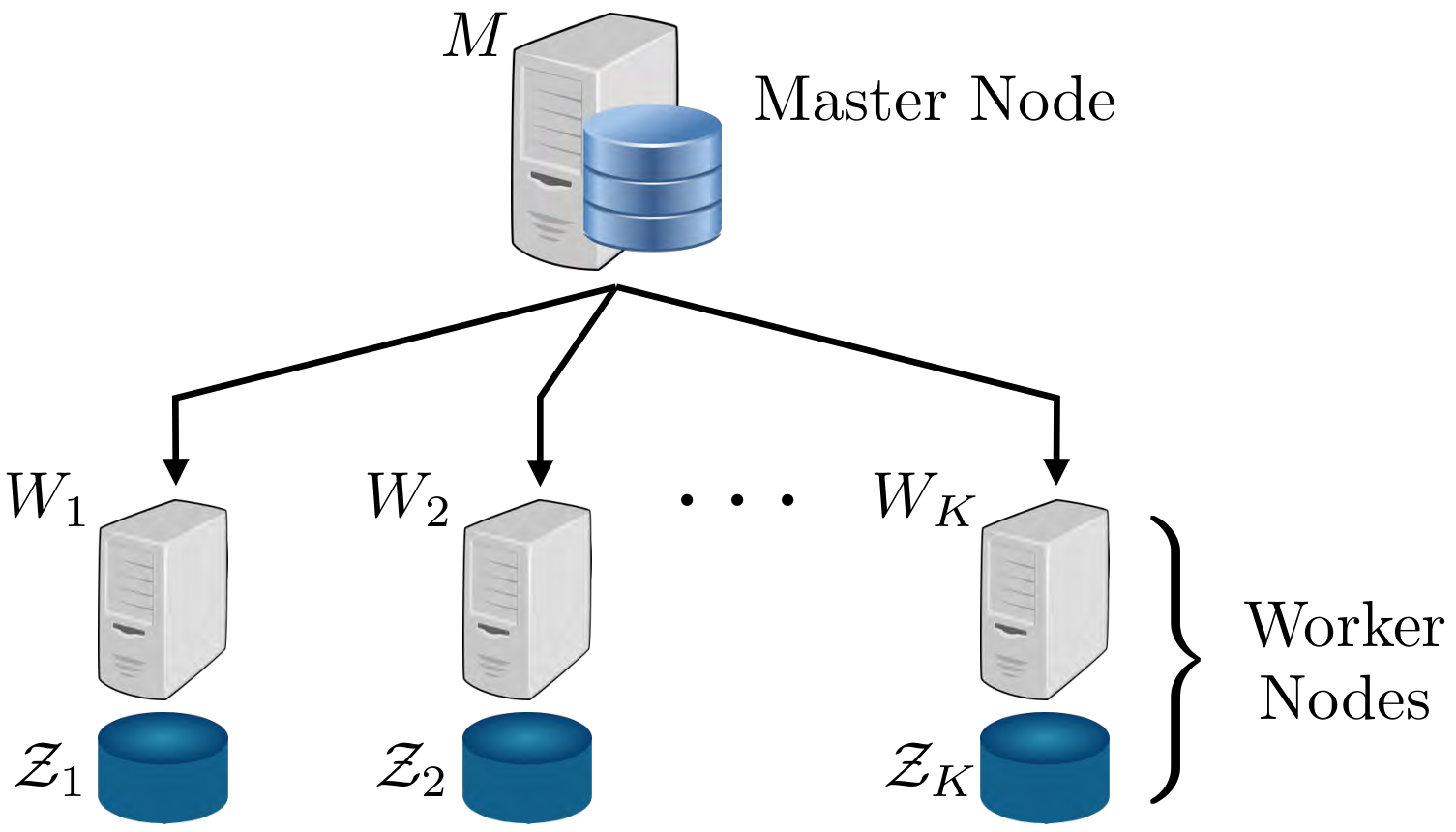
Fig. 1: Data shuffling in a distributed computing system.

For an integer KK, let [K]\left[K\right] denote the set of integers {1,2,…,K}\left\{1,2,\ldots,K\right\}. Fig. 1 depicts a distributed computing system with a master node, denoted by MM, and a set of KK worker nodes, denoted by 𝒲={Wi:i∈[K]}\mathcal{W}=\{W_{i}:i\in[K]\}. The master node is assumed to have access to a data-set, including NN files, denoted by ℱ={Fj:j∈[N]}\mathcal{F}=\{F^{j}:j\in[N]\}, where the size of each file is normalized to 11 unit. In practice, the number of files is remarkably larger than the number of worker nodes, and hence we study the data shuffling problem under the practical assumption of N≥KN\geq K. At each iteration, each worker node should perform a local computational task on a subset of N/KN/K files44 4 Unless otherwise stated, we assume that N/KN/K and S/(N/K)S/(N/K) are integers.. The assignment of files to worker nodes is done by the master node, either randomly or according to some predefined mechanism. Each worker node WiW_{i} has a cache 𝒵i\mathcal{Z}_{i} that can store up to SS files, including those N/KN/K under-processing files. This imposes the constraint S≥N/KS\geq N/K on the size of the cache at each worker node. Once the computation at the worker nodes is done, the result is sent back to the master node. A new batch of N/KN/K files will be assigned to each worker node for iteration t+1t+1, and the cache contents of the worker nodes should be accordingly modified. The communication of files from the master node to the worker nodes occurs over a shared link, i.e., any information sent by the master node will be received by all of the worker nodes. Similar to [15, 17, 18, 16], the broadcast communication channel between the master node and worker nodes is assumed to be perfect.

For a given iteration tt, we denote by u⁡(i)u(i) the set of indices of the files to be processed by WiW_{i}, and by 𝒫i\mathcal{P}^{i} the portion of the cache of WiW_{i} dedicated to the under-processing files: 𝒫i={Fj:j∈u⁡(i)}\mathcal{P}^{i}=\{F^{j}:j\in u(i)\}. The subsets {u⁡(i):i∈[K]}\{u(i):i\in[K]\} provide a partitioning for the set of file indices, i.e., u⁡(i)∩u⁡(j)=∅u(i)\cap u(j)=\varnothing for i≠ji\neq j, and ⋃i=1Ku⁡(i)=[N]\bigcup_{i=1}^{K}u(i)=[N]. Similarly, d⁡(i)d(i) denotes the subset of indices of N/KN/K files to be processed by WiW_{i} at iteration t+1t+1, where {d⁡(i):i∈[K]}\{d(i):i\in[K]\} also forms a partitioning for [N][N]. When S>N/KS>N/K, each worker node has an excess storage to cache (parts of) the other files in ℱ\mathcal{F}, in addition to the N/KN/K files in 𝒫i\mathcal{P}^{i}. We denote by ℰi=𝒵i∖𝒫i\mathcal{E}_{i}=\mathcal{Z}_{i}\setminus\mathcal{P}^{i} the contents of the remaining space of the cache of WiW_{i}, which is called the excess storage. Therefore, 𝒵i=𝒫i∪ℰi\mathcal{Z}_{i}=\mathcal{P}^{i}\cup\mathcal{E}_{i}. Let 𝒫i​(t)\mathcal{P}^{i}(t), ℰi​(t)\mathcal{E}_{i}(t) and 𝒵i​(t)\mathcal{Z}_{i}(t) denote the realizations of 𝒫i\mathcal{P}^{i}, ℰi\mathcal{E}_{i} and 𝒵i\mathcal{Z}_{i} at iteration tt, respectively. For the sake of brevity, we may drop the iteration index tt whenever it is clear from the context.

Filling the excess part of the caches of worker nodes is performed independently of the new assigned subsets {d⁡(i):i∈[K]}\{d(i):i\in[K]\}. Between iterations tt and t+1t+1, the master node should compute and broadcast a message (a function of all files in ℱ\mathcal{F}), such that each worker node WiW_{i} can retrieve all files in d⁡(i)d(i) from its cached data 𝒵i\mathcal{Z}_{i} and the broadcast message 𝒳\mathcal{X}. The communication load R=R⁡(K,N,S)R=R(K,N,S) is defined as the size of the broadcast message 𝒳\mathcal{X} for the parameters introduced above. We interchangeably refer to RR as delivery load and communication load of the underlying data-shuffling system. The goal is to develop a cache placement strategy and design a broadcast message 𝒳\mathcal{X} to minimize RR for any {d⁡(i):i∈[K]}\{d(i):i\in[K]\}. For S≥NS\geq N, we have R=0R=0 since each worker node can store all the files in its cache and no communication is needed between the master node and worker nodes for any shuffling. Thus, we can focus on the regime of N/K≤S≤NN/K\leq S\leq N. We define S^=S/(N/K)\widehat{S}=S/(N/K) to be the cache size normalized by the size of data to be processed by each worker node. Accordingly, we have 1≤S^≤K1\leq\widehat{S}\leq K.

Refer to caption
(a)
Refer to caption
(b)
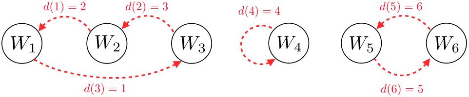
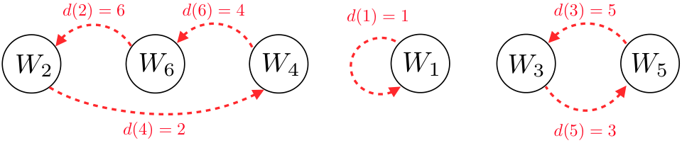
Fig. 2: The file transition graphs for two instances of a data shuffling system with K=6K=6 worker nodes and N=6N=6 files. Assume u⁡(i)=iu(i)=i for i∈[6]i\in[6], and consider two different assignment functions; d1​(⋅)d_{1}(\cdot) and d2​(⋅)d_{2}(\cdot). The shown graphs are isomorphic. (a) d1​(1)=2,d1​(2)=3,d1​(3)=1,d1​(4)=4,d1​(5)=6d_{1}(1)=2,d_{1}(2)=3,d_{1}(3)=1,d_{1}(4)=4,d_{1}(5)=6 and d1​(6)=5d_{1}(6)=5. (b) d2​(1)=1,d2​(2)=6,d2​(3)=5,d2​(4)=2,d2​(5)=3d_{2}(1)=1,d_{2}(2)=6,d_{2}(3)=5,d_{2}(4)=2,d_{2}(5)=3 and d2​(6)=4d_{2}(6)=4.

II-B File Transition Graph

A file transition graph is defined as a directed graph 𝒢⁡(V,E)\mathcal{G}(V,E), where VV, with |V|=K|V|=K, denotes the set of vertices each corresponding to a worker node, and EE, with |E|=N|E|=N, is the set of directed edges, each associated to one file (see Fig. 2). An edge ej=(i,ℓ)∈Ee_{j}=(i,\ell)\in E with j∈[N]j\in[N] and i,ℓ∈[K]i,\ell\in[K] indicates that j∈u⁡(i)∩d⁡(ℓ)j\in u(i)\cap d(\ell), i.e., file FjF^{j} is being processed by worker node WiW_{i} at iteration tt, and assigned to worker node WℓW_{\ell} to be processed at iteration t+1t+1. Note that in general 𝒢⁡(V,E)\mathcal{G}(V,E) is a multigraph, since there might be multiple files in u⁡(i)∩d⁡(ℓ)u(i)\cap d(\ell), and we include one edge from WiW_{i} to WℓW_{\ell} for each of such files.

Without loss of generality, let us assume a fixed assignment function u⁡(⋅)u(\cdot) at iteration tt, for example, u⁡(i)={(i−1)​N/K+ℓ:ℓ∈[N/K]}u(i)=\{(i-1)N/K+\ell:\ell\in[N/K]\} for i∈[K]i\in[K], otherwise we can relabel the files. Hence, the problem and its file transition graph are fully determined by the assignment function d⁡(⋅)d(\cdot) at iteration t+1t+1. Let 𝒟𝒢\mathcal{D}_{\mathcal{G}} be the set of assignment functions d⁡(⋅)d(\cdot) whose corresponding file transition graphs are isomorphic to 𝒢\mathcal{G}. Fig. 2 captures two instances of a shuffling problem with isomorphic file transition graphs. For a given graph 𝒢⁡(V,E)\mathcal{G}(V,E), we define the average delivery load over all assignment functions in 𝒟𝒢\mathcal{D}_{\mathcal{G}} as

R⁡(𝒢)=1|𝒟𝒢|​∑d∈𝒟𝒢R⁡(N,K,S,d).\displaystyle R(\mathcal{G})=\frac{1}{|\mathcal{D}_{\mathcal{G}}|}\sum_{d\in\mathcal{D}_{\mathcal{G}}}R(N,K,S;d). (1)

Our ultimate goal in this paper is to characterize R⁡(𝒢)R(\mathcal{G}) for given parameter (N,K,S)(N,K,S) and for all feasible file transition graphs 𝒢\mathcal{G}.

II-C Main Results

First, we present our main results to characterize the exact load-memory trade-off for the canonical setting of data shuffling problem, when N=KN=K, for any shuffling. Since N=KN=K, then S^=S\widehat{S}=S, each worker node processes one file at each iteration. Without loss of generality, we assume that WiW_{i} processes file FiF^{i} at every iteration, i.e., u⁡(i)=iu(i)=i, for i∈[K]i\in[K], otherwise we can relabel the files. The following theorems summarize our main results.

Theorem 1.

For a data shuffling problem with a master node, KK worker nodes, each with a cache of size SS files with S∈[N]S\in[N], the communication load R=R⁡(N=K,K,S)R=R(N=K,K,S) required to shuffle N=KN=K files among the worker nodes for any file transition graph is upper bounded by55 5 Note that (nk)=0\binom{n}{k}=0 when n<kn<k.

R\displaystyle R ≤\displaystyle\leq (K−1S)(K−1S−1).\displaystyle\frac{\binom{K-1}{S}}{\binom{K-1}{S-1}}. (2)

For non-integer values of SS, where 1≤S≤N1\leq S\leq N, the lower convex envelope of the NN corner points, characterized by (2), is achievable by memory-sharing.

An achievability argument consists of a cache placement strategy and a delivery scheme. We propose a cache placement in Section III which will be used for all achievable schemes discussed in this paper. The delivery scheme, along with the memory-sharing argument for non-integer values of SS, is presented in Section IV-A. Illustrative examples are then given in Section IV-B.

The next theorem provides an achievable delivery load (depending on the file transition graph) by an opportunistic coding scheme. We will show later that the underlying file transition graph of any data shuffling problem, 𝒢⁡(V,E)\mathcal{G}(V,E), comprises a number of directed cycles. We denote the number of cycles in the file transition graph by γ\gamma, and denote the cycle lengths by (ℓ1,ℓ2,…,ℓγ)(\ell_{1},\ell_{2},\dots,\ell_{\gamma}) where ∑i=1γℓi=K\sum_{i=1}^{\gamma}\ell_{i}=K.

Theorem 2.

For a data shuffling system with a master node and KK worker nodes, each with a cache of size SS files, for S∈[N]S\in[N], the shuffling of N=KN=K files among the worker nodes for a given file transition graph that comprises γ\gamma cycles can be performed by broadcasting a message of size RR, where

R\displaystyle R ≤\displaystyle\leq (K−1S)−(γ−1S)(K−1S−1).\displaystyle\frac{\binom{K-1}{S}-\binom{\gamma-1}{S}}{\binom{K-1}{S-1}}. (3)

For non-integer values of SS, where 1≤S≤N1\leq S\leq N, the lower convex envelope of the NN corner points, characterized by (3), is achievable by memory-sharing.

The proposed delivery scheme and achievability proof for Theorem 2 are presented in Section IV-C. The memory-sharing argument for non-integer values of SS follows a similar reasoning as the one in Theorem 1. We provide an illustrative example in Section IV-D.

Theorem 3.

For the data shuffling system introduced in Theorem 2, the communication load RR required to shuffle N=KN=K files among the worker nodes for a given assignment with a file transition graph that comprises γ\gamma cycles is lower bounded by

R\displaystyle R ≥\displaystyle\geq (K−1S)−(γ−1S)(K−1S−1).\displaystyle\frac{\binom{K-1}{S}-\binom{\gamma-1}{S}}{\binom{K-1}{S-1}}. (4)

The proof of optimality (converse) is presented in Section V, where we also provide an illustrative example to describe the proof technique.

Corollary 1.

Theorems 2 and 3 prove the optimality of the proposed coded shuffling scheme for an arbitrary number of worker nodes KK, storage capacity per worker node SS, and file transition graph with γ\gamma cycles, when N=KN=K. Therefore, the optimal delivery load R⋆R^{\star} is characterized as

R⋆​(N=K,K,S)\displaystyle R^{\star}(N=K,K,S) =\displaystyle= (K−1S)−(γ−1S)(K−1S−1),S∈[N].\displaystyle\frac{\binom{K-1}{S}-\binom{\gamma-1}{S}}{\binom{K-1}{S-1}},\quad S\in[N]. (5)

For non-integer values of SS, where 1≤S≤N1\leq S\leq N, the optimal delivery load R⋆R^{\star} is equal to the lower convex envelope of the NN corner points given in (5). Furthermore, when γ−1<S\gamma-1<S, the achievable delivery load of Theorem 2 is equal to that of Theorem 1, and takes its maximum. This characterizes the optimal worst-case delivery load Rworst-case⋆R^{\star}_{\text{worst-case}} which is given by

Rworst-case⋆\displaystyle R^{\star}_{\text{worst-case}} =\displaystyle= (K−1S)(K−1S−1).\displaystyle\frac{\binom{K-1}{S}}{\binom{K-1}{S-1}}. (6)

This indicates that the upper bound of Theorem 1 is the best universal (assignment independent) bound that holds for all instances of the data shuffling problem.

Remark 1.

The essence of the information-theoretic lower bound on the communication load for the worst-case shuffling proposed in this paper for N=KN=K is equivalent to that of [16] (Attia et al.) for general NN and KK. However, in more details, the proof of [16] involves solving a linear program, while we use set theoretic arguments to obtain a closed-form expression. Moreover, for general parameters NN and KK, we provide a simple reduction argument to re-use the bound proved for the canonical setting.

Fig. 3 captures the optimum trade-off curve between R⋆​(K,K,S)R^{\star}(K,K,S) as a function of SS for N=K=6N=K=6 and a file transition graph with γ=3\gamma=3 cycles.

Fig. 3: The optimum trade-off curve between the delivery load R⋆R^{\star} and the storage capacity per worker node SS, when N=K=6N=K=6 and γ=3\gamma=3.

Next, based on the results obtained for the canonical setting of data shuffling problem when N=KN=K, we present our main results in Theorem 4 to characterize an upper bound on the load-memory trade-off for the general setting of data shuffling problem when N≥KN\geq K. This upper bound turns out to be optimum for the worst-case shuffling, as stated in Theorem 5.

Theorem 4.

For a data shuffling system that processes NN files, and consists of a master node and KK worker nodes, each with a normalized storage capacity of S^=S/(N/K)\widehat{S}=S/(N/K) files, the achievable delivery load R=R⁡(N,K,S)R=R(N,K,S) required to shuffle NN files among the worker nodes for any file transition graph is upper bounded by

R\displaystyle\displaystyle R ≤\displaystyle\leq NK​(K−1S^)(K−1S^−1),S^∈[K].\displaystyle\frac{N}{K}\frac{\binom{K-1}{\widehat{S}}}{\binom{K-1}{\widehat{S}-1}},\quad\widehat{S}\in[K]. (7)

For non-integer values of S^\widehat{S}, where 1≤S^≤K1\leq\widehat{S}\leq K, the lower convex envelope of the NN corner points, characterized by (7) is achievable by memory-sharing.

The delivery scheme and achievability proof are presented in Section VI-A. Note that the proposed achievable scheme is an extension to the one developed for the canonical setting of N=KN=K in Theorem 2. The memory-sharing argument for non-integer values of S^\widehat{S} follows a similar reasoning as the one in Theorem 1. We also present an illustrative example in Section VI-C.

Theorem 5.

For the data shuffling system introduced in Theorem 4, the communication load Rworst-caseR_{\textrm{worst-case}} required to shuffle NN files among the worker nodes according to the worst-case shuffling is given by

Rworst-case\displaystyle\displaystyle R_{\textrm{worst-case}} =\displaystyle= NK​(K−1S^)(K−1S^−1).\displaystyle\frac{N}{K}\frac{\binom{K-1}{\widehat{S}}}{\binom{K-1}{\widehat{S}-1}}. (8)

The proof of Theorem 5 is presented in Section VI-D.

Before we start discussing the results of the paper, we present an example to explain the general idea of the proposed coded shuffling scheme.

II-D Illustrative Example

Example 1 (Single-Cycle File Transition Graph): Consider a shuffling system with a master node and K=4K=4 worker nodes. The size of the cache at each worker node is S=2S=2 files. There are N=4N=4 files, denoted by {F1,F2,F3,F4}\{F^{1},F^{2},F^{3},F^{4}\}. For notational simplicity, we rename the files as {A,B,C,D}\{A,B,C,D\}. Without loss of generality, we assume that worker nodes W1W_{1}, W2W_{2}, W3W_{3} and W4W_{4} are processing files AA, BB, CC, and DD, respectively, at iteration tt, that is u⁡(1)=Au(1)=A, u⁡(2)=Bu(2)=B, u⁡(3)=Cu(3)=C, and u⁡(4)=Du(4)=D. The file transition graph is d⁡(1)=Bd(1)=B, d⁡(2)=Cd(2)=C, d⁡(3)=Dd(3)=D and d⁡(4)=Ad(4)=A, as depicted by Fig. 4a.

(a)
Refer to caption
(b)
(c)
(d)
Refer to caption
(e)
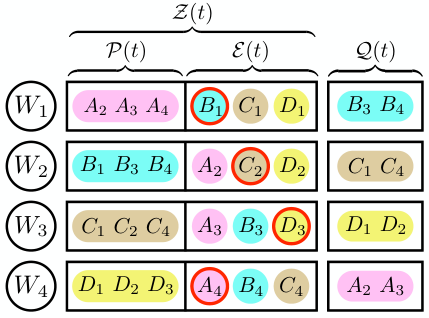
Fig. 4: Data shuffling system with N=K=4N=K=4, S=2S=2 and γ=1\gamma=1. (a) The file transition graph for a data shuffling system with N=K=4N=K=4, S=2S=2 and γ=1\gamma=1. Worker nodes W1W_{1}, W2W_{2}, W3W_{3} and W4W_{4} are processing files AA, BB, CC, and DD, respectively. (b) Cache organization of worker nodes at iteration tt, along with the set of subfiles which are not available in the caches at iteration tt and need to be processed at iteration t+1t+1. (c) Cache organization of worker nodes at iteration t+1t+1 after updating the caches. Subfiles A4A_{4}, B1B_{1}, C2C_{2} and D3D_{3} in ℰ4​(t)\mathcal{E}_{4}(t), ℰ1​(t)\mathcal{E}_{1}(t), ℰ2​(t)\mathcal{E}_{2}(t) and ℰ3​(t)\mathcal{E}_{3}(t) are moved to ℰ1​(t+1)\mathcal{E}_{1}(t+1), ℰ2​(t+1)\mathcal{E}_{2}(t+1), ℰ3​(t+1)\mathcal{E}_{3}(t+1) and ℰ4​(t+1)\mathcal{E}_{4}(t+1), respectively. (d) Cache organization of worker nodes at iteration t+1t+1 after updating the caches and relabeling the subfiles of Fig. 4b. Subfiles A4A_{4}, B1B_{1}, C2C_{2} and D3D_{3} in ℰ4​(t)\mathcal{E}_{4}(t), ℰ1​(t)\mathcal{E}_{1}(t), ℰ2​(t)\mathcal{E}_{2}(t) and ℰ3​(t)\mathcal{E}_{3}(t) are moved to ℰ1​(t+1)\mathcal{E}_{1}(t+1), ℰ2​(t+1)\mathcal{E}_{2}(t+1), ℰ3​(t+1)\mathcal{E}_{3}(t+1) and ℰ4​(t+1)\mathcal{E}_{4}(t+1) and relabeled to D1′D_{1}^{\prime}, A2′A_{2}^{\prime}, B3′B_{3}^{\prime} and C4′C_{4}^{\prime}, respectively. (e) Received functions by worker nodes after removing the cached subfiles. The complete received functions at worker nodes are expressed in (9).

The proposed placement strategy partitions each file into (K−1S−1)=3\binom{K-1}{S-1}=3 subfiles of equal sizes. The subfiles are labeled with sets Γ⊆[4]\Gamma\subseteq[4], where |Γ|=S^−1=S/(N/K)−1=1|\Gamma|=\widehat{S}-1=S/(N/K)-1=1. For instance, file AA being processed by worker node W1W_{1} is partitioned into A2A_{2}, A3A_{3}, and A4A_{4}. Accordingly, the cache 𝒵i\mathcal{Z}_{i} of WiW_{i} is divided into two parts; 𝒫i\mathcal{P}^{i} that is dedicated to the under-processing file FiF^{i}, and ℰi\mathcal{E}_{i} that is dedicated to store parts of other files. Fig. 4b captures the cache organization of worker nodes, along with the missing subfiles (i.e., the ones in 𝒬i\mathcal{Q}_{i}, as defined in (14)) that need to be processed at iteration t+1t+1. The broadcast message 𝒳\mathcal{X} transmitted from the master node to the worker nodes is formed by the concatenation of 33 sub-messages 𝒳=(X12,X13,X23)\mathcal{X}=(X_{12},X_{13},X_{23}), where

X12=A2⊕B3⊕B4⊕C1,X13=A3⊕B3⊕C1⊕D1,X23=B3⊕C1⊕C4⊕D2.\displaystyle\begin{split}X_{12}&=A_{2}\oplus B_{3}\oplus B_{4}\oplus C_{1},\\ X_{13}&=A_{3}\oplus B_{3}\oplus C_{1}\oplus D_{1},\\ X_{23}&=B_{3}\oplus C_{1}\oplus C_{4}\oplus D_{2}.\end{split} (9)

We need to show that each worker node WiW_{i} can decode all the missing subfiles in 𝒬i\mathcal{Q}_{i} from the broadcast message. Fig. 4e shows the received sub-messages by each worker node after removing the subfiles that exist in its cache. For instance, W1W_{1} can decode B3B_{3} from X13X_{13} and B4B_{4} from X13⊕X12X_{13}\oplus X_{12}, respectively. These, together with B1B_{1} that is already cached in 𝒵1\mathcal{Z}_{1}, enable W1W_{1} to fully recover BB, which is the file to be processed at iteration t+1t+1.

Decoding file AA at W4W_{4}, which is the ignored worker node, is more involved. Worker node W4W_{4} can decode A2A_{2} and A3A_{3} from X12⊕X23X_{12}\oplus X_{23} and X13⊕X23X_{13}\oplus X_{23}, respectively, and A4A_{4} already exists in its cache 𝒵4\mathcal{Z}_{4}. Consequently, the proposed scheme can achieve a delivery load of Rcoded=1R_{\text{coded}}=1, due to sending 33 sub-messages, each of size 1/31/3. On the other hand, the delivery load achieved by the uncoded shuffling scheme, under the same placement strategy, involves sending 88 sub-messages, each of size 1/31/3, resulting in Runcoded=8/3R_{\text{uncoded}}=8/3. Hence, the proposed coded shuffling scheme can save around 62%62\% of the communication load, compared to the uncoded shuffling scheme.

After the decoding phase, each worker node has access to (at least) 88 subfiles, including 66 subfiles pre-stored in its cache 𝒵i\mathcal{Z}_{i}, and 22 subfiles in 𝒬i\mathcal{Q}_{i}. However, only 66 subfiles can be stored in the cache, and the remaining ones should be discarded. It remains to show that the caches of the worker nodes can be updated using the broadcast message 𝒳\mathcal{X} to maintain a similar arrangement in preparation for the next data shuffle from iteration t+1t+1 to t+2t+2. This is done in two phases, namely cache updating and subfile relabeling. Fig. 4c depicts the cache organization of the worker nodes after updating the caches, while Fig. 4d captures the cache organization of the worker nodes after updating the caches and relabeling the subfiles. For example, as shown in Fig. 4c, W1W_{1} needs to keep a full copy of B={B1,B2,B3}B=\{B_{1},B_{2},B_{3}\} at iteration t+1t+1 because d⁡(1)=Bd(1)=B. Moreover, subfiles C1C_{1} and D1D_{1} already exist in ℰ1​(t)\mathcal{E}_{1}(t), and hence they will remain in ℰ1​(t+1)\mathcal{E}_{1}(t+1). Among the remaining subfiles {A2,A3,A4}\{A_{2},A_{3},A_{4}\}, only one of them can be kept in the cache. According to (20), the subfile to be kept is AΓA_{\Gamma} such that d−1​(1)∈Γd^{-1}(1)\in\Gamma, that is A4A_{4}. Finally, in order to maintain a cache configuration consistent with the original one in (11), all the subfiles in the excess storage of WiW_{i} should have a subscript of {i}\{i\}, and WiW_{i} should process FiF_{i}, for i∈[K]i\in[K], at every iteration. For example, subfiles B1B_{1}, B3B_{3} and B4B_{4}, that are processed in 𝒫1​(t+1)\mathcal{P}^{1}{}(t+1) by W1W_{1}, in Fig. 4c are relabeled to A2′A_{2}^{\prime}, A3′A_{3}^{\prime} and A4′A_{4}^{\prime} in Fig. 4d, respectively. Similarly, subfiles C1C_{1}, D1D_{1}, A4A_{4}, that are cached in ℰ1​(t+1)\mathcal{E}_{1}(t+1) by W1W_{1}, in Fig. 4c are relabeled to B1′B_{1}^{\prime}, C1′C_{1}^{\prime} and D1′D_{1}^{\prime} in Fig. 4d, respectively. ⧫\blacklozenge

III Cache Placement

In this section we introduce our proposed cache placement, in which the contents of each worker node’s cache at iteration tt are known. Note that the cache placement does not depend on the files to be processed by the worker nodes at iteration t+1t+1, i.e., it does not depend on {d⁡(i):i∈[K]}\{d(i):i\in[K]\}.

III-A File Partitioning and Labeling

Throughout this work, we assume that N/KN/K and S/(N/K)S/(N/K) are integer numbers, unless it is specified otherwise. Let S^=S/(N/K)\widehat{S}=S/(N/K). Let FjF^{j} be a file being processed by worker node WiW_{i} at iteration tt, i.e., j∈u⁡(i)j\in u(i). We partition FjF^{j} into (K−1S^−1)\binom{K-1}{\widehat{S}-1} equal-size subfiles, and label the subfiles with a subscript as

Fj={FΓj:Γ⊆[K]∖{i},|Γ|=S^−1},∀i∈[K],j∈[N],j∈u(i).\displaystyle F^{j}=\{F^{j}_{\Gamma}:\Gamma\subseteq[K]\setminus\{i\},|\Gamma|=\widehat{S}-1\},\>\>\forall i\in[K],\>j\in[N],\>j\in u(i). (10)

Since the size of each file is normalized to 11, the size of each subfile will be 1/(K−1S^−1)1/\binom{K-1}{\widehat{S}-1}. For the sake of completeness, we also define dummy subfiles FΓj=0F^{j}_{\Gamma}=0 (with size 00) for every Γ⊆[K]\Gamma\subseteq[K] with j∈Γj\in\Gamma or |Γ|≠S^−1|\Gamma|\neq\widehat{S}-1.

III-B Cache Placement

The cache 𝒵i\mathcal{Z}_{i} of WiW_{i} consists of two parts: (i) the under-processing part 𝒫i\mathcal{P}^{i}, in which all subfiles of files to be processed at iteration tt are stored; (ii) the excess storage part ℰi\mathcal{E}_{i}, which is equally distributed among all other files. We denote by ℰiℓ\mathcal{E}_{i}^{\ell} the portion of ℰi\mathcal{E}_{i} dedicated to the file FℓF^{\ell}, in which all subfiles FΓℓF^{\ell}_{\Gamma} with i∈Γi\in\Gamma are cached. Hence, we have

𝒵i\displaystyle\mathcal{Z}_{i} =\displaystyle= 𝒫i∪ℰi=𝒫i∪(⋃ℓ∈[N]∖u⁡(i)ℰiℓ),∀i∈[K],\displaystyle\mathcal{P}^{i}\cup\mathcal{E}_{i}=\mathcal{P}^{i}\cup\left(\bigcup\nolimits_{\ell\in[N]\setminus u(i)}\mathcal{E}_{i}^{\ell}\right),\>\>\forall i\in[K], (11)

where

𝒫i\displaystyle\mathcal{P}^{i} =\displaystyle= {FΓj:j∈u(i),Γ⊆[K]∖{i},|Γ|=S^−1},\displaystyle\left\{F^{j}_{\Gamma}:j\in u(i),\>\Gamma\subseteq[K]\setminus\{i\},\>|\Gamma|=\widehat{S}-1\right\}, (12)
ℰiℓ\displaystyle\mathcal{E}_{i}^{\ell} =\displaystyle= {FΓℓ:ℓ∉u(i),i∈Γ⊆[K],|Γ|=S^−1}.\displaystyle\left\{F^{\ell}_{\Gamma}:\ell\notin u(i),\>i\in\Gamma\subseteq[K],\>|\Gamma|=\widehat{S}-1\right\}. (13)

For any worker node WiW_{i}, there are N/KN/K complete files in 𝒫i\mathcal{P}^{i}. Moreover, for each of the remaining N−N/KN-N/K files, there are (K−2S^−2)\binom{K-2}{\widehat{S}-2} subfiles, out of a total of (K−1S^−1)\binom{K-1}{\widehat{S}-1} subfiles, that are cached in the excess storage part. Thus, we have

|𝒵i|=|𝒫i|+∑ℓ∈[N]∖u⁡(i)|ℰiℓ|=NK+(N−NK)​(K−2S^−2)(K−1S^−1)=S,\displaystyle\displaystyle|\mathcal{Z}_{i}|=\left|\mathcal{P}^{i}\right|+\sum_{\ell\in[N]\setminus u(i)}\left|\mathcal{E}_{i}^{\ell}\right|=\frac{N}{K}+\left(N-\frac{N}{K}\right)\frac{\binom{K-2}{\widehat{S}-2}}{\binom{K-1}{\widehat{S}-1}}=S,

which satisfies the memory constraints.

Remark 2.

The proposed cache placement is different from the one in [14] (Lee et al.). The placement in [15] follows a random sampling of the files independently across the users. Moreover, file splitting is not allowed in [15], and a file (data point) is either fully stored in the storage of a worker node, or no bit of that is cached by the worker node. The proposed placement strategy, however, is deterministic and fully characterized at every shuffling iteration. On the other hand, the so-called structural invariant placement strategy introduced in [16] is deterministic, but different from the one proposed in this paper. In particular, the structural invariant placement method works for values of S^\widehat{S} satisfying S^=(1+i⁡(K−1K))\widehat{S}=\left(1+i\left(\frac{K-1}{K}\right)\right) for some integer i=0,1,…,Ki=0,1,\dots,K, while we need S^\widehat{S} to be some integer in [K][K]. Consequently, the communication load achieved in [16] is sub-optimum for general KK. A variation of the structural invariant storage placement is proposed in [16, Appendix D] only for S^∈{1,K−2,K−1}\widehat{S}\in\{1,K-2,K-1\} which is identical the placement strategy proposed in our work for any integer value of S^\widehat{S}. It is worth noting that in spite of similarities between the placement strategies, the proposed encoding and decoding methods in [16] (referred to as “aligned coded shuffling”) are completely different from those proposed in this paper.

Recall that the worker node WiW_{i} should be able to recover files {Fℓ:ℓ∈d⁡(i)}\{F^{\ell}:\ell\in d(i)\} from its cache 𝒵i\mathcal{Z}_{i} and the broadcast message 𝒳\mathcal{X}. Communicating files in d⁡(i)d(i) from the master node to a worker node WiW_{i} can be limited to sending only the desired subfiles that do not exist in the cache of WiW_{i}. For a worker node i∈[K]i\in[K], let 𝒬i\mathcal{Q}_{i} denote the set of subfiles to be processed by WiW_{i} at iteration t+1t+1, which are not available in its cache 𝒵i\mathcal{Z}_{i} at iteration tt, that is,

𝒬i={FΓℓ:ℓ∈d(i),ℓ∉u(i),i∉Γ,Γ⊆[K],|Γ|=S^−1}.\displaystyle\mathcal{Q}_{i}=\left\{F^{\ell}_{\Gamma}:\ell\in d(i),\>\ell\notin u(i),\>i\notin\Gamma,\>\Gamma\subseteq[K],\>|\Gamma|=\widehat{S}-1\right\}. (14)

It is evident that each worker node needs to decode at most (K−1S^−1)−(K−2S^−2)=(K−2S^−1)\binom{K-1}{\widehat{S}-1}-\binom{K-2}{\widehat{S}-2}=\binom{K-2}{\widehat{S}-1} subfiles for each of the N/KN/K files in d⁡(i)d(i), in order to process them at iteration t+1t+1.

The pseudocodes of the proposed file partitioning and labeling, and cache placement are given in Algorithm 1 and Algorithm 2, respectively, in Appendix H.

IV Coded Shuffling for the Canonical Setting (N=K)(N=K)

We describe two delivery strategies in this section. The first delivery scheme is universal, in the sense that it does not exploit the properties of the underlying file transition graph. By analyzing this scheme in Section IV-A, we show that the delivery load in Theorem 1 is achievable. Two illustrative examples are presented in Section IV-B to better describe the coding and decoding strategies. We then demonstrate that the size of the broadcast message can be reduced by exploiting the cycles in the file transition graph. A graph-based delivery strategy is proposed in Section IV-C. This new scheme can achieve the reduced delivery load proposed in Theorem 2. Finally, we conclude this section by presenting an illustrative example for the graph-based delivery scheme in Section IV-D.

IV-A A Universal Delivery Scheme for Any Shuffling: Proof of Theorem 1

Recall that for N=KN=K we have S^=S/(N/K)=S\widehat{S}=S/(N/K)=S. In order to prove Theorem 1, we propose a coded shuffling scheme to show that a delivery load of R=(K−1S)/(K−1S−1)R=\binom{K-1}{S}/\binom{K-1}{S-1} is achievable for the canonical setting (N=KN=K) for any integer 1≤S≤N1\leq S\leq N. We assume, without loss of generality, that WiW_{i} processes file FiF^{i} at iteration tt, i.e., u⁡(i)=iu(i)=i for i∈[K]i\in[K], otherwise we can relabel the files.

Encoding

Given all cache contents {𝒵i:i∈[K]}\{\mathcal{Z}_{i}:i\in[K]\}, characterized by (11), and {d⁡(i):i∈[K]}\{d(i):i\in[K]\}, the broadcast message 𝒳\mathcal{X} sent from the master node to the worker nodes is obtained by the concatenation of a number of sub-messages XΔX_{\Delta}, each specified for a group of worker nodes Δ\Delta, that is,

𝒳\displaystyle\mathcal{X} =\displaystyle= {XΔ:Δ⊆[K−1],|Δ|=S},\displaystyle\{X_{\Delta}:\Delta\subseteq[K-1],|\Delta|=S\}, (15)

where

XΔ≜⨁i∈Δ(FΔ∖{i}i⊕FΔ∖{d⁡(i)}d⁡(i)⊕⨁j∈[K]∖ΔF({j}∪Δ)∖{i,d⁡(i)}d⁡(i)).\displaystyle X_{\Delta}\triangleq\bigoplus_{i\in\Delta}\left(F^{i}_{\Delta\setminus\{i\}}\oplus F^{d(i)}_{\Delta\setminus\{d(i)\}}\oplus\bigoplus_{j\in[K]\setminus\Delta}F^{d(i)}_{(\{j\}\cup\Delta)\setminus\{i,d(i)\}}\right). (16)

The encoding design hinges on K−1K-1 worker nodes. Without loss of generality, we consider W1,W2,…,WK−1W_{1},W_{2},\ldots,W_{K-1} for whom the broadcast sub-messages are designed, and designate WKW_{K} as the ignored worker node. We will later show how WKW_{K} is served for free using the sub-messages designed for other worker nodes.

Remark 3.

It is true that subfile FΔ∖{d⁡(i)}d⁡(i)F^{d(i)}_{\Delta\setminus\{d(i)\}} does exist in the cache of worker node WiW_{i}, and is not needed to be broadcast, and indeed the encoded sub-message does not include this subfile. This is due to the fact that such a subfile FΔ∖{d⁡(i)}d⁡(i)F^{d(i)}_{\Delta\setminus\{d(i)\}} appears twice in XΔX_{\Delta}, and hence will be canceled by the XOR operation. Note that, this subfile is not dummy only if d⁡(i)∈Δd(i)\in\Delta. Therefore, one copy is attained in the second term of the summand as FΔ∖{d⁡(i)}d⁡(i)F^{d(i)}_{\Delta\setminus\{d(i)\}}, and the second copy is attained as the first term in the summand as FΔ∖{j}jF^{j}_{\Delta\setminus\{j\}} for j=d⁡(i)∈Δj=d(i)\in\Delta.

According to the proposed encoding scheme, there are a total of (K−1S)\binom{K-1}{S} encoded sub-messages, each corresponds to one subset Δ\Delta, and the size of each sub-message is 1/(K−1S−1)1/\binom{K-1}{S-1}. Hence, the overall broadcast communication load is upper bounded by

R\displaystyle R ≤\displaystyle\leq (K−1S)(K−1S−1),\displaystyle\frac{\binom{K-1}{S}}{\binom{K-1}{S-1}},

as claimed in Theorem 1.

Decoding

The following lemmas demonstrate how each worker node decodes the missing subfiles, that constitute the file to be processed at iteration t+1t+1, from the broadcast sub-messages and its cache contents.

Lemma 1.

For a worker node WℓW_{\ell}, where ℓ∈[K−1]\ell\in[K-1], a missing subfile FΓd⁡(ℓ)∈𝒬ℓF^{d(\ell)}_{\Gamma}\in\mathcal{Q}_{\ell} can be decoded

  • •

    from 𝒵ℓ\mathcal{Z}_{\ell} and the broadcast sub-message X{ℓ}∪ΓX_{\{\ell\}\cup\Gamma}, if K∉ΓK\notin\Gamma; and

  • •

    from 𝒵ℓ\mathcal{Z}_{\ell}, the broadcast sub-message X(Γ∖{K})∪{ℓ,d⁡(ℓ)}X_{(\Gamma\setminus\{K\})\cup\{\ell,d(\ell)\}}, and other subfiles previously decoded by WℓW_{\ell}, if K∈ΓK\in\Gamma.

We refer to Appendix A for the proof of lemma 1.

Remark 4.

Here, we provide an intuitive justification for Lemma 1. Consider a worker node WiW_{i} and a set of worker nodes Δ\Delta of size SS that includes ii. One can show that every subfile appearing in XΔX_{\Delta} belongs to either 𝒵i\mathcal{Z}_{i} or 𝒬i\mathcal{Q}_{i}. Therefore, worker node WiW_{i} can recover a linear equation in the subfiles in 𝒬i\mathcal{Q}_{i} by removing the subfiles in its cache 𝒵i\mathcal{Z}_{i} from XΔX_{\Delta}. It turns out that all such equations are linearly independent. The number of such equations is (K−2S−1)\binom{K-2}{S-1} (because Δ⊆[K−1]\Delta\subseteq[K-1] and i∈Δi\in\Delta). On the other hand, the number of subfiles in 𝒬i\mathcal{Q}_{i} is (at most) (K−1S−1)−(K−2S−2)=(K−2S−1)\binom{K-1}{S-1}-\binom{K-2}{S-2}=\binom{K-2}{S-1}, since out of a total of (K−1S−1)\binom{K-1}{S-1} subfiles of Fd⁡(i)F^{d(i)}, (K−2S−2)\binom{K-2}{S-2} of them are cached in ℰid⁡(i)\mathcal{E}_{i}^{d(i)}, characterized by (13). Therefore, the obtained set of linearly independent equations suffices to recover all the subfiles in 𝒬i\mathcal{Q}_{i}.

Lemma 2.

For the worker node WKW_{K}, any missing subfile FΓd⁡(K)∈𝒬KF^{d(K)}_{\Gamma}\in\mathcal{Q}_{K} can be decoded from the cache contents 𝒵K\mathcal{Z}_{K} and the summation of the broadcast sub-messages ⨁ℓ∈[K−1]∖ΓX{ℓ}∪Γ\displaystyle\bigoplus_{\ell\in[K-1]\setminus\Gamma}X_{\{\ell\}\cup\Gamma}.

We refer to Appendix B for the proof of lemma 2.

Cache Updating and Subfile Relabeling

After worker nodes decode the missing subfiles, characterized by (14), the caches of worker nodes need to be updated and the subfiles need to be relabeled before processing the files at iteration t+1t+1. The goal of cache updating and subfile relabeling is to maintain a similar cache configuration for the worker nodes for shuffling iteration t+2t+2. First, the caches are updated as follows:

  • •

    For i∈[K]i\in[K], all the subfiles of Fd⁡(i)F^{d(i)} are placed in 𝒫i\mathcal{P}^{i} at iteration t+1t+1, i.e.,

    𝒫i​(t+1)\displaystyle\mathcal{P}^{i}(t+1) =\displaystyle= {FΓd⁡(i):Γ⊆[K]∖{d(i)},|Γ|=S−1}.\displaystyle\left\{F^{d(i)}_{\Gamma}:\Gamma\subseteq[K]\setminus\{d(i)\},\>|\Gamma|=S-1\right\}. (17)
  • •

    For i∈[K]i\in[K], the excess storage is updated by removing all the subfiles of Fd⁡(i)F^{d(i)}, and replacing them by the subfiles of FiF^{i} that were cached at Wd−1​(i)W_{d^{-1}(i)}, i.e.,

    ℰi​(t+1)\displaystyle\mathcal{E}_{i}(t+1) =\displaystyle= (ℰi​(t)∖𝒮i)∪𝒜i,\displaystyle\left(\mathcal{E}_{i}(t)\setminus\mathcal{S}_{i}\right)\cup\mathcal{A}_{i}, (18)

    where

    𝒮i\displaystyle\mathcal{S}_{i} =\displaystyle= {FΓd⁡(i):i∈Γ,Γ⊆[K]∖{d(i)},|Γ|=S−1},\displaystyle\left\{F^{d(i)}_{\Gamma}:i\in\Gamma,\>\Gamma\subseteq[K]\setminus\{d(i)\},\>|\Gamma|=S-1\right\}, (19)
    𝒜i\displaystyle\mathcal{A}_{i} =\displaystyle= {FΓi:d−1(i)∈Γ,Γ⊆[K]∖{i},|Γ|=S−1}.\displaystyle\left\{F^{i}_{\Gamma}:d^{-1}(i)\in\Gamma,\>\Gamma\subseteq[K]\setminus\{i\},\>|\Gamma|=S-1\right\}. (20)

Consequently, we have 𝒵i​(t+1)=𝒫i​(t+1)∪ℰi​(t+1)\mathcal{Z}_{i}(t+1)=\mathcal{P}^{i}(t+1)\cup\mathcal{E}_{i}(t+1) by definition. Note that the cache updating procedure is feasible, since the subfiles needed for 𝒵i​(t+1)\mathcal{Z}_{i}(t+1) either exist in 𝒵i​(t)\mathcal{Z}_{i}(t) or appear in the set of missing subfiles 𝒬i​(t)\mathcal{Q}_{i}(t) to be decoded after the broadcast message delivery. In particular, all the subfiles of FiF^{i} already exist in 𝒫i​(t)\mathcal{P}^{i}(t), and hence those in 𝒜i\mathcal{A}_{i} will be simply moved from the under-processing part to the excess storage part of the cache.

Next, the subfiles are relabeled as follows:

  1. 1.

    For every subfile FΓiF^{i}_{\Gamma}, where i∈[K]i\in[K], d−1​(i)∈Γd^{-1}(i)\in\Gamma, Γ⊆[K]∖{i}\Gamma\subseteq[K]\setminus\{i\} and |Γ|=S−1|\Gamma|=S-1, relabel the subfile’s subscript to FΛiF^{i}_{\Lambda}, where Λ=(Γ∖{d−1​(i)})∪{i}\Lambda=\left(\Gamma\setminus\left\{d^{-1}(i)\right\}\right)\cup\left\{i\right\}.

  2. 2.

    For every subfile FΓiF^{i}_{\Gamma}, where i∈[K]i\in[K], Γ⊆[K]∖{i}\Gamma\subseteq[K]\setminus\{i\} and |Γ|=S−1|\Gamma|=S-1, relabel the subfile’s superscript to FΓd−1​(i)F^{d^{-1}(i)}_{\Gamma}.

At the end of cache updating and subfile relabeling phase, the cache configuration of each worker node at iteration t+1t+1 maintains a similar arrangement to that introduced initially at iteration tt and characterized by (11). More specifically, the cache updating step ensures that the under-processing part of the cache includes all subfiles of the file to be processed at iteration t+1t+1. It also guarantees that the excess storage part of the cache stores an equal share of subfiles of all other files that are not in the under-processing part. The subfile relabeling step, however, ensures that two properties are satisfied at any shuffling iteration; (i) the index of a worker node appears in the new subscript of all subfiles in the excess storage part of its cache, (ii) the name of the file to be processed by worker node WiW_{i} is changed to FiF^{i} (from Fd⁡(i)F^{d(i)}). Therefore, the proposed scheme can be systematically applied at the following shuffling iterations. This completes the proof of Theorem 1. ■\blacksquare

The pseudocodes of the proposed encoding at the master node, decoding at the worker nodes, and cache updating and subfile relabeling are given in Algorithm 3, Algorithm 4, and Algorithm 5, respectively, in Appendix H.

Remark 5.

Let SS be a non-integer cache size with 1≤S≤N1\leq S\leq N. We can always write S=α⁡⌊S⌋+(1−α)​⌈S⌉S=\alpha\lfloor S\rfloor+\left(1-\alpha\right)\lceil S\rceil, for some α∈(0,1)\alpha\in(0,1). The data shuffling problem for non-integer cache size SS can be addressed by a memory-sharing argument, similar to [17]. More precisely, we can show that the pairs (⌊S⌋,R⁡(⌊S⌋))\left(\lfloor S\rfloor,R\left(\lfloor S\rfloor\right)\right) and (⌈S⌉,R⁡(⌈S⌉))\left(\lceil S\rceil,R\left(\lceil S\rceil\right)\right) are achievable, and conclude that, for S=α⁡⌊S⌋+(1−α)​⌈S⌉S=\alpha\lfloor S\rfloor+\left(1-\alpha\right)\lceil S\rceil, a communication load of R⁡(S)=α​R​(⌊S⌋)+(a−α)​R​(⌈S⌉)R\left(S\right)=\alpha R\left(\lfloor S\rfloor\right)+(a-\alpha)R\left(\lceil S\rceil\right) can be achieved. Recall that the size of each file is normalized to 11 unit. For the memory-sharing argument, each file will be partitioned into two parts of sizes α\alpha and 1−α1-\alpha. The cache of each worker node is also divided into two parts of sizes α​S\alpha S and (1−α)​S(1-\alpha)S. Then, the files of size α\alpha will be cached and shuffled within the parts of the caches of size α​S\alpha S. Similarly, the files of size 1−α1-\alpha, together with the parts of the caches of size (1−α)​S(1-\alpha)S, form another isolated instance of the problem. Summing the delivery loads of the two instances, we get

R⁡(α⁡⌊S⌋+(1−α)​⌈S⌉)\displaystyle R(\alpha\lfloor S\rfloor+\left(1-\alpha\right)\lceil S\rceil) =\displaystyle= α​R​(⌊S⌋)+(1−α)​R​(⌈S⌉)\displaystyle\alpha R(\lfloor S\rfloor)+\left(1-\alpha\right)R(\lceil S\rceil) (21)
≤\displaystyle\leq α​(K−1⌊S⌋)−(γ−1⌊S⌋)(K−1⌊S⌋−1)+(1−α)​(K−1⌈S⌉)−(γ−1⌈S⌉)(K−1⌈S⌉−1).\displaystyle\alpha\frac{\binom{K-1}{\lfloor S\rfloor}-\binom{\gamma-1}{\lfloor S\rfloor}}{\binom{K-1}{\lfloor S\rfloor-1}}+\left(1-\alpha\right)\frac{\binom{K-1}{\lceil S\rceil}-\binom{\gamma-1}{\lceil S\rceil}}{\binom{K-1}{\lceil S\rceil-1}}.

This shows that the convex hull of the pairs {(S,R):S∈[N]}\{(S,R):S\in[N]\} is achievable.

Refer to caption
Fig. 5: The file transition graph for a data shuffling system with N=K=6N=K=6 and γ=3\gamma=3. Worker nodes W1W_{1}, W2W_{2}, W3W_{3}, W4W_{4}, W5W_{5} and W6W_{6} process files AA, BB, CC, DD, EE, and FF at iteration tt, respectively.

IV-B Illustrative Examples

Example 2 (Multiple-Cycle File Transition Graph): Consider a shuffling problem with parameters K=6K=6, S=3S=3, and N=6N=6. For simplicity, we rename the files {F1,F2,F3,F4,F5,F5}\{F^{1},F^{2},F^{3},F^{4},F^{5},F^{5}\} to {A,B,C,D,E,F}\{A,B,C,D,E,F\}. Assume worker nodes W1W_{1}, W2W_{2}, W3W_{3}, W4W_{4}, W5W_{5} and W6W_{6} are processing files AA, BB, CC, DD, EE, and FF, respectively. The file transition graph is depicted by Fig. 5. It comprises γ=3\gamma=3 cycles, with cycle lengths (ℓ1,ℓ2,ℓ3)=(3,1,2)(\ell_{1},\ell_{2},\ell_{3})=(3,1,2). That is, d⁡(1)=Bd(1)=B, d⁡(2)=Cd(2)=C, d⁡(3)=Ad(3)=A in the first cycle, d⁡(4)=Dd(4)=D in the second cycle, and d⁡(5)=Fd(5)=F, d⁡(6)=Ed(6)=E in the third cycle. Fig. 6a captures the cache organization of worker nodes, along with the missing subfiles that need to be processed at the next iteration. Note that 𝒫i\mathcal{P}^{i} and ℰi\mathcal{E}_{i}, for i∈[K]i\in[K], are designed according to (12) and (13), respectively. We use (15) and (16) to design the broadcast message 𝒳\mathcal{X}, which is constructed by concatenating a number of XΔX_{\Delta}, each intended for S=3S=3 worker nodes. For example, X123X_{123} is expressed as

X123\displaystyle X_{123} =\displaystyle= ⨁i∈{1,2,3}(F{1,2,3}∖{i}i⊕F{1,2,3}∖{d⁡(i)}d⁡(i)⊕⨁j∈[K]∖{1,2,3}F({j}∪{1,2,3})∖{i,d⁡(i)}d⁡(i))\displaystyle\bigoplus_{i\in\{1,2,3\}}\left(F^{i}_{\{1,2,3\}\setminus\{i\}}\oplus F^{d(i)}_{\{1,2,3\}\setminus\{d(i)\}}\oplus\bigoplus_{j\in[K]\setminus\{1,2,3\}}F^{d(i)}_{(\{j\}\cup\{1,2,3\})\setminus\{i,d(i)\}}\right) (22)
=\displaystyle= (F231⊕F132⊕(F342⊕F352⊕F362))⊕(F132⊕F123⊕(F143⊕F153⊕F163))⊕(F123⊕F231⊕(F241⊕F251⊕F261))\displaystyle\left(F^{1}_{23}\oplus F^{2}_{13}\oplus\left(F^{2}_{34}\oplus F^{2}_{35}\oplus F^{2}_{36}\right)\right)\oplus\left(F^{2}_{13}\oplus F^{3}_{12}\oplus\left(F^{3}_{14}\oplus F^{3}_{15}\oplus F^{3}_{16}\right)\right)\oplus\left(F^{3}_{12}\oplus F^{1}_{23}\oplus\left(F^{1}_{24}\oplus F^{1}_{25}\oplus F^{1}_{26}\right)\right)
=\displaystyle= F241⊕F251⊕F261⊕F342⊕F352⊕F362⊕F143⊕F153⊕F163\displaystyle F^{1}_{24}\oplus F^{1}_{25}\oplus F^{1}_{26}\oplus F^{2}_{34}\oplus F^{2}_{35}\oplus F^{2}_{36}\oplus F^{3}_{14}\oplus F^{3}_{15}\oplus F^{3}_{16}
=\displaystyle= A24⊕A25⊕A26⊕B34⊕B35⊕B36⊕C14⊕C15⊕C16.\displaystyle A_{24}\oplus A_{25}\oplus A_{26}\oplus B_{34}\oplus B_{35}\oplus B_{36}\oplus C_{14}\oplus C_{15}\oplus C_{16}.

Similarly, the set of other broadcast sub-messages is expressed as

X124=A24⊕B34⊕B45⊕B46⊕C14,X125=A25⊕B35⊕B45⊕B56⊕C15⊕E12⊕F12,X134=A24⊕A45⊕A46⊕B34⊕C14,X135=A25⊕A45⊕A56⊕B35⊕C15⊕E13⊕F13,X145=A45⊕B45⊕E14⊕F14,X234=A24⊕B34⊕C14⊕C45⊕C46,X235=A25⊕B35⊕C15⊕C45⊕C56⊕E23⊕F23,X245=B45⊕C45⊕E24⊕F24,X345=A45⊕C45⊕E34⊕F34.\displaystyle\begin{split}X_{124}&=A_{24}\oplus B_{34}\oplus B_{45}\oplus B_{46}\oplus C_{14},\\ X_{125}&=A_{25}\oplus B_{35}\oplus B_{45}\oplus B_{56}\oplus C_{15}\oplus E_{12}\oplus F_{12},\\ X_{134}&=A_{24}\oplus A_{45}\oplus A_{46}\oplus B_{34}\oplus C_{14},\\ X_{135}&=A_{25}\oplus A_{45}\oplus A_{56}\oplus B_{35}\oplus C_{15}\oplus E_{13}\oplus F_{13},\\ X_{145}&=A_{45}\oplus B_{45}\oplus E_{14}\oplus F_{14},\\ X_{234}&=A_{24}\oplus B_{34}\oplus C_{14}\oplus C_{45}\oplus C_{46},\\ X_{235}&=A_{25}\oplus B_{35}\oplus C_{15}\oplus C_{45}\oplus C_{56}\oplus E_{23}\oplus F_{23},\\ X_{245}&=B_{45}\oplus C_{45}\oplus E_{24}\oplus F_{24},\\ X_{345}&=A_{45}\oplus C_{45}\oplus E_{34}\oplus F_{34}.\end{split} (23)

It should be noted that no subfiles of file DD appears in any of the sub-messages defined (23) since u⁡(4)=d⁡(4)=Du(4)=d(4)=D, i.e., DD is processed by W4W_{4} at iterations tt and t+1t+1, and hence does not need to be transmitted by the master node for this data shuffle. Moreover, note that index 66 does not appear in the subscript of the broadcast sub-messages, since W6W_{6} is the ignored worker node. However, the subfiles assigned to W6W_{6} can be recovered by linear combination of other transmitted sub-messages.

(a)
(b)
(c)
Fig. 6: Data shuffling system with N=K=6N=K=6, S=3S=3 and γ=3\gamma=3. The file transition graph is depicted in Fig. 5. (a) Cache organization of worker nodes at iteration tt, along with the set of subfiles which are not available in the caches at iteration tt and need to be processed at iteration t+1t+1. (b) Cache organization of worker nodes at iteration t+1t+1 after updating the caches. For instance, subfiles {B13,B14,B15,B16}\left\{B_{13},B_{14},B_{15},B_{16}\right\} in ℰ1​(t)\mathcal{E}_{1}(t) are moved to ℰ2​(t+1)\mathcal{E}_{2}(t+1). (c) Received functions by worker nodes after removing the cached subfiles. The complete received functions at worker nodes are expressed in (22) and (23).

For each worker node, Fig. 6c shows the received sub-messages from the master node after removing the subfiles that already exist in its cache. The decoding procedure of the proposed coded shuffling scheme is analogous to interference mitigation techniques in wireless communications. To present this analogy, we focus on three different cases of the decoding procedure.

(i) Decoding C14C_{14} from X124X_{124} by W2W_{2}:

X124\displaystyle X_{124} =\displaystyle= C14⏟Desired subfile⊕A24⊕B34⊕B45⊕B46⏟Cached subfiles in 𝒵2.\displaystyle\underbrace{C_{14}}_{\text{Desired subfile}}\oplus\underbrace{A_{24}\oplus B_{34}\oplus B_{45}\oplus B_{46}}_{\text{Cached subfiles in $\mathcal{Z}_{2}$}}.

The decoding procedure is analogous to interference suppression technique. W2W_{2} decodes C14C_{14} by canceling the interfering subfiles using its cache contents 𝒵2\mathcal{Z}_{2}.

(ii) Decoding C16C_{16} from X123X_{123} by W2W_{2}:

X123\displaystyle X_{123} =\displaystyle= C16⏟Desired subfile⊕C14⏟Decoded subfilefrom X124⊕C15⏟Decoded subfilefrom X125⊕A24⊕A25⊕A26⊕B34⊕B35⊕B36⏟Cached subfiles in 𝒵2.\displaystyle\underbrace{C_{16}}_{\text{Desired subfile}}\oplus\underbrace{C_{14}}_{\begin{subarray}{c}\text{Decoded subfile}\\ \text{from $X_{124}$}\end{subarray}}\oplus\underbrace{C_{15}}_{\begin{subarray}{c}\text{Decoded subfile}\\ \text{from $X_{125}$}\end{subarray}}\oplus\underbrace{A_{24}\oplus A_{25}\oplus A_{26}\oplus B_{34}\oplus B_{35}\oplus B_{36}}_{\text{Cached subfiles in $\mathcal{Z}_{2}$}}.

The decoding procedure is analogous to successive interference cancellation (SIC) technique. W2W_{2} decodes C16C_{16} by first canceling the subfiles that exist in 𝒵2\mathcal{Z}_{2}. Next, it exploits the subfiles decoded from X124X_{124} and X125X_{125} to successively cancel the remaining interfering subfiles.

(iii) Decoding E23E_{23} from X235X_{235} by W6W_{6}:

X235\displaystyle X_{235} =\displaystyle= E23⏟Desired subfile⊕(C56⊕F23)⏟Cached subfilesin 𝒵6⊕(A25⊕B35⊕C15⊕C45)⏟X123⊕X234.\displaystyle\underbrace{E_{23}}_{\text{Desired subfile}}\oplus\underbrace{\left(C_{56}\oplus F_{23}\right)}_{\begin{subarray}{c}\text{Cached subfiles}\\ \text{in $\mathcal{Z}_{6}$}\end{subarray}}\oplus\underbrace{\left(A_{25}\oplus B_{35}\oplus C_{15}\oplus C_{45}\right)}_{\text{$X_{123}\oplus X_{234}$}}.

The decoding procedure is analogous to aligned interference suppression (interference alignment) technique. W6W_{6} decodes E23E_{23} by first canceling the subfiles cached in 𝒵6\mathcal{Z}_{6}. Then, the remaining interfering subfiles are the result of XORing some other received sub-messages, i.e., X123⊕X234X_{123}\oplus X_{234}, and hence, they can be canceled accordingly.

As a result, the achieved delivery load is Rcoded=(53)/(52)=1R_{\text{coded}}=\binom{5}{3}/\binom{5}{2}=1. On the other hand, the delivery load achieved by the uncoded shuffling scheme, under the same placement strategy, is Runcoded=(5×6)/(52)=3R_{\text{uncoded}}=(5\times 6)/\binom{5}{2}=3. That is, the proposed coded shuffling scheme can save around 66%66\% of the communication load, and thus, it speeds up the overall run-time of the data shuffling process. When each worker node decodes all missing subfiles at iteration tt, Fig. 6b depicts the cache organization of each worker node after updating the cache in preparation for the following data shuffle at iteration t+1t+1. Note that the subfiles can be relabeled in a similar way as in Example 11. ⧫\blacklozenge

IV-C A Graph-Based Delivery Scheme for Any Shuffling: Proof of Theorem 2

The coded shuffling scheme proposed in Section IV-A provides the worker nodes with the missing parts of their assigned files, using the broadcast message and cached subfiles. However, depending on the file transition graph, the delivery load obtained by that scheme may be sub-optimum. As an extreme and hypothetical example, consider a file transition graph where each worker node WiW_{i} is assigned the same file to process at iterations tt and t+1t+1, i.e., d⁡(i)=u⁡(i)d(i)=u(i). Clearly, no communication between the master node and worker nodes is needed in this case, and hence, R=0R=0 is achievable. This implies the scheme in Section IV-A is sub-optimal for this instance of the shuffling problem.

It turns out that the number of cycles in the file transition graph is the main characteristic to determine the optimum delivery scheme. More concretely, for a file transition graph with γ\gamma cycles where γ−1≥S\gamma-1\geq S, we show that there are precisely (γ−1S)\binom{\gamma-1}{S} sub-messages in (15) that are linearly dependent on the other sub-messages. Thus, by refraining from broadcasting these sub-messages, we can reduce the delivery load, and achieve the one given in (3). In the decoding phase, worker nodes can first recover all the redundant sub-messages that have not been transmitted by the master node by computing linear combinations of appropriate sub-messages that have been received. Then, each worker node follows the same decoding rules, discussed in Section IV, to decode the assigned file at iteration t+1t+1. This results in an opportunistic coded shuffling scheme based on the scheme proposed in Section IV-A. We will later show in Section V that this scheme is indeed optimum, and achieves the minimum possible delivery load.

The following lemma characterizes the linearly dependent sub-messages, and quantifies the reduced delivery load:

Lemma 3.

Consider a data shuffling system with a master node, KK worker nodes with storage capacity per worker node SS, and N=KN=K files, and a given file transition graph that comprises γ\gamma cycles. Consider the placement strategy given in Section III and the delivery scheme provided in Section IV-A. Then, there are a total of (γ−1S)\binom{\gamma-1}{S} redundant (linearly dependent) sub-messages among the (K−1S)\binom{K-1}{S} broadcasting sub-messages.

We refer to Appendix C for the proof of lemma 3.

In fact, we can explicitly characterize the set of redundant sub-messages that are not broadcast in the delivery phase. To this end,

  • •

    consider the first γ−1\gamma-1 cycles out of the total of γ\gamma cycles formed by the file transition graph (generally, we have to consider all cycles except the one that includes the ignored worker node);

  • •

    from these γ−1\gamma-1 cycles, consider all possible combinations of sets of cycles that have SS distinct cycles. There are (γ−1S)\binom{\gamma-1}{S} such sets;

  • •

    consider all sub-messages XΔX_{\Delta} (defined in (16)) where Δ\Delta has exactly one worker node from each of the chosen SS cycles.

In the proof of Lemma 3, we show that the sum of all such sub-messages is zero. Thus, the master node can remove one of the sub-messages from each group and transmit the rest of them to the worker nodes. Therefore, the resulting broadcast communication load RR is upper bounded by

R\displaystyle R ≤\displaystyle\leq (K−1S)−(γ−1S)(K−1S−1).\displaystyle\frac{\binom{K-1}{S}-\binom{\gamma-1}{S}}{\binom{K-1}{S-1}}.

In the decoding phase, each worker node first reconstructs the missing, redundant sub-messages by adding the other sub-messages in the group, and then follows the same decoding scheme, and cache updating and subfile relabeling strategies introduced in Section IV-A. This completes the proof of Theorem 2. In the next example, we illustrate the concept of redundancy within the the set of broadcast sub-messages.

IV-D Illustrative Example

Example 3 (Multiple-Cycle File Transition Graph with Opportunistic Transmission):

Fig. 7: Cache organization of worker nodes at iteration tt, along with the set of subfiles which are not available in the caches at iteration tt and need to be processed at iteration t+1t+1, for a data shuffling system with N=K=6N=K=6, S=2S=2 and γ=3\gamma=3. The file transition graph for this system is depicted in Fig. 5.

We consider the same system parameters of Example 2 in Section IV-B with the same file transition graph given in Fig. 5, except that here the cache size of each worker node is S=2S=2 files. Fig. 7 captures the cache organization of worker nodes, along with the missing subfiles that need to be processed at iteration t+1t+1. Following the achievable scheme proposed in IV-A, the set of sub-messages transmitted by the master node to the worker nodes is expressed as

X12=A2⊕B3⊕B4⊕B5⊕B6⊕C1,X13=A2⊕A4⊕A5⊕A6⊕B3⊕C1,X14=A4⊕B4,X15=A5⊕B5⊕E1⊕F1,X23=A2⊕B3⊕C1⊕C4⊕C5⊕C6,X24=B4⊕C4,X25=B5⊕C5⊕E2⊕F2,X34=A4⊕C4,X35=A5⊕C5⊕E3⊕F3,X45=E4⊕F4.\displaystyle\begin{split}X_{12}&=A_{2}\oplus B_{3}\oplus B_{4}\oplus B_{5}\oplus B_{6}\oplus C_{1},\\ X_{13}&=A_{2}\oplus A_{4}\oplus A_{5}\oplus A_{6}\oplus B_{3}\oplus C_{1},\\ X_{14}&=A_{4}\oplus B_{4},\\ X_{15}&=A_{5}\oplus B_{5}\oplus E_{1}\oplus F_{1},\\ X_{23}&=A_{2}\oplus B_{3}\oplus C_{1}\oplus C_{4}\oplus C_{5}\oplus C_{6},\\ X_{24}&=B_{4}\oplus C_{4},\\ X_{25}&=B_{5}\oplus C_{5}\oplus E_{2}\oplus F_{2},\\ X_{34}&=A_{4}\oplus C_{4},\\ X_{35}&=A_{5}\oplus C_{5}\oplus E_{3}\oplus F_{3},\\ X_{45}&=E_{4}\oplus F_{4}.\end{split} (24)

Note that the file transition graph consists of γ=3\gamma=3 cycles, namely, {W1,W2,W3}\{W_{1},W_{2},W_{3}\}, {W4}\{W_{4}\}, and {W5,W6}\{W_{5},W_{6}\}, where the ignored worker node W6W_{6} appears in the third cycle. Ignoring the third cycle, we have two remaining ones. The family of all Δ\Delta’s with exactly one entry from each of the first and second cycle is given by {{1,4},{2,4},{3,4}}\{\{1,4\},\{2,4\},\{3,4\}\}. It is evident that X14X_{14}, X24X_{24} and X34X_{34} are linearly dependent, since X34⊕X14⊕X24=0X_{34}\oplus X_{14}\oplus X_{24}=0. Therefore, we can safely omit X34X_{34} from the set of the transmitted sub-messages. For decoding purposes, worker nodes can recover X34X_{34} from X14X_{14} and X24X_{24}. Therefore, each one of them is able to decode the assigned file at iteration t+1t+1 by following the decoding procedure presented in Section IV. ⧫\blacklozenge

V Converse Proof for Data Shuffling with Canonical Setting (N=K)(N=K)

We prove the optimality of the coded shuffling scheme proposed in Section IV-C, as stated in Theorem 3. The instance of the problem is fully determined by the indices of files to be processed by the worker nodes at iterations tt and t+1t+1, i.e., u⁡(⋅)u(\cdot) and d⁡(⋅)d(\cdot), respectively. Without loss of generality, we may assume u⁡(i)=iu(i)=i for every i∈[K]i\in[K], otherwise we can relabel the files. These assignment functions induce a directed file transition graph 𝒢⁡(V,E)\mathcal{G}(V,E), with node set V={W1,W2,…,WK}V=\{W_{1},W_{2},\dots,W_{K}\}, in which there is an edge from WiW_{i} to WjW_{j} if and only if d⁡(Wj)=Fid(W_{j})=F^{i}.

Since the in-degrees and out-degrees of each vertex are equal to 11, such a graph consists of a number of directed cycles. Let γ\gamma denote the number of cycles in this graph with cycle lengths given by {ℓ1,ℓ2,…,ℓγ}\{\ell_{1},\ell_{2},\dots,\ell_{\gamma}\}. Then each node in the graph can be represented by a pair (c,p)(c,p), where c∈{1,2,…,γ}c\in\{1,2,\dots,\gamma\} denoted the cycle number, and p∈{1,2,…,ℓc}p\in\{1,2,\dots,\ell_{c}\} denotes the position within cycle cc. With this notation66 6 The selection of the order of cycles, as well as the starting position within each cycle, is arbitrary., we have d⁡(c,p)=u⁡(c,p+1)=(c,p+1)d(c,p)=u(c,p+1)=(c,p+1), i.e., the worker node at position (c,p)(c,p) will process file F(c,p)F^{(c,p)} and F(c,p+1)F^{(c,p+1)} at iterations tt and t+1t+1, respectively77 7 We define (c,ℓc+1)=(c,1)(c,\ell_{c}+1)=(c,1) for the sake of consistency.. Note that the positional label (c,p)(c,p) essentially induces an order on the nodes and edges of the graph. For two pairs (c′,p′)(c^{\prime},p^{\prime}) and (c,p)(c,p), we say (c′,p′)(c^{\prime},p^{\prime}) appears before (c,p)(c,p) and denote it by (c′,p′)≺(c,p)(c^{\prime},p^{\prime})\prec(c,p) if either (c′,p′)(c^{\prime},p^{\prime}) appears in a cycle with smaller index (c′<cc^{\prime}<c) or in the same cycle but at an smaller position (c′=cc^{\prime}=c and p′<pp^{\prime}<p). Similarly, (c′,p′)⪯(c,p)(c^{\prime},p^{\prime})\preceq(c,p) indicates that either (c′,p′)≺(c,p)(c^{\prime},p^{\prime})\prec(c,p) or (c′,p′)=(c,p)(c^{\prime},p^{\prime})=(c,p).

Consider an arbitrary uncoded placement of the files in worker nodes’ cache, and denote by F~ji\widetilde{F}^{i}_{j} the bits of file FiF^{i} cached at WjW_{j}. Note that we do not make any assumptions on the size or symmetry of F~ji\widetilde{F}^{i}_{j}’s. Then, the cache contents of worker node WjW_{j} is given by 𝒵j=Fj∪⋃i≠jF~ji\mathcal{Z}_{j}=F^{j}\cup\bigcup_{i\neq j}\widetilde{F}^{i}_{j}, which is equivalent to

𝒵(c,p)=F(c,p)∪(⋃(c′,p′)≠(c,p)F~(c,p)(c′,p′)),\displaystyle\mathcal{Z}_{(c,p)}=F^{(c,p)}\cup\left(\bigcup_{(c^{\prime},p^{\prime})\neq(c,p)}\widetilde{F}^{(c^{\prime},p^{\prime})}_{(c,p)}\right), (25)

using the positional labeling, where jj is the worker node in the ppth position of the ccth cycle.

For a given file transition graph 𝒢⁡(V,E)\mathcal{G}(V,E), we introduce a virtual worker node W⋆W_{\star} equipped with a cache 𝒵⋆\mathcal{Z}_{\star}, in which we store

𝒵⋆\displaystyle\mathcal{Z}_{\star} =\displaystyle= (⋃c∈[γ]F(c,1))∪(⋃c∈[γ]p<ℓc(⋃(c′,p′)≻(c,p)p′>1F~(c,p)(c′,p′)))\displaystyle\left(\bigcup_{c\in\left[\gamma\right]}F^{(c,1)}\right)\cup\left(\bigcup_{\begin{subarray}{c}c\in\left[\gamma\right]\\ p<\ell_{c}\end{subarray}}\left(\bigcup_{\begin{subarray}{c}(c^{\prime},p^{\prime})\succ(c,p)\\ p^{\prime}>1\end{subarray}}\widetilde{F}^{(c^{\prime},p^{\prime})}_{(c,p)}\right)\right) (26)
=\displaystyle= (⋃c∈[γ]F(c,1))∪(⋃c∈[γ]p>1(⋃(c′,p′)≺(c,p)p′<ℓc′F~(c′,p′)(c,p))),\displaystyle\left(\bigcup_{c\in\left[\gamma\right]}F^{(c,1)}\right)\cup\left(\bigcup_{\begin{subarray}{c}c\in\left[\gamma\right]\\ p>1\end{subarray}}\left(\bigcup_{\begin{subarray}{c}(c^{\prime},p^{\prime})\prec(c,p)\\ p^{\prime}<\ell_{c^{\prime}}\end{subarray}}\widetilde{F}^{(c,p)}_{(c^{\prime},p^{\prime})}\right)\right), (27)

where

  • •

    in (26), the first equality reads as follows. the cache 𝒵⋆\mathcal{Z}_{\star} of the virtual worker node W⋆W_{\star} is the union of two sets. The first set is the union of files being processed by the first worker node in each cycle. The second set only consists the sub-files of all other files, and only includes sub-files that are stored at worker nodes that (i) whose rank is the circular order is less that that of the processing worker, and (ii) do not appear at the last position of their cycle.

  • •

    in (27), the second equality in (25) is just a re-arrangement of the sub-files selected in (24). That will follows form two steps applied simultaneously, i.e., (i) swapping the labels used for the subscript and superscripts of F~\widetilde{F}, and (ii) changing the order of the unions.

In order to prove the optimality of the proposed coded shuffling scheme, we first show that the broadcast message 𝒳\mathcal{X} and the cache contents of the virtual worker node suffice to decode all the files (Lemma 4). Then, we lower bound the size of the broadcast message by upper bounding the size of the data cached at the virtual worker node (Lemma 5 and Lemma 6).

Lemma 4.

For any file transition graph GG, given the cache contents 𝒵⋆\mathcal{Z}_{\star} of the virtual worker node W⋆W_{\star} and the broadcast message 𝒳\mathcal{X}, all files in the data shuffling system can be decoded, that is

H⁡({Fi}i=1K|𝒳,𝒵⋆)\displaystyle H\left(\{F^{i}\}_{i=1}^{K}|\mathcal{X},\mathcal{Z}_{\star}\right) =\displaystyle= 0.\displaystyle 0. (28)

We refer to Appendix D for the proof of Lemma 4.

For a file FiF^{i} and a subset of worker nodes 𝒥⊆[K]∖{i}\mathcal{J}\subseteq[K]\setminus\{i\}, we define the size of a union of bits of FiF^{i} that are cached at worker nodes in 𝒥\mathcal{J} as μ𝒥i=|⋃j∈𝒥F~ji|\mu^{i}_{\mathcal{J}}=\left|\bigcup\nolimits_{j\in\mathcal{J}}\widetilde{F}^{i}_{j}\right|. For a given integer α\alpha, let μα\mu_{\alpha} denote the average (over files and worker nodes) size of a set of union of bits that are cached in the excess storage of α\alpha worker nodes, that is,

μα\displaystyle\mu_{\alpha} =\displaystyle= 1K​(K−1α)​∑i∈[K]∑𝒥⊆[K]∖i|𝒥|=αμ𝒥i\displaystyle\frac{1}{K\binom{K-1}{\alpha}}\sum_{i\in[K]}\sum_{\begin{subarray}{c}\mathcal{J}\subseteq[K]\setminus i\\ |\mathcal{J}|=\alpha\end{subarray}}\mu^{i}_{\mathcal{J}} (29)
=\displaystyle= 1K​(K−1α)​∑i∈[K]∑𝒥⊆[K]∖i|𝒥|=α|⋃j∈𝒥F~ji|.\displaystyle\frac{1}{K\binom{K-1}{\alpha}}\sum_{i\in[K]}\sum_{\begin{subarray}{c}\mathcal{J}\subseteq[K]\setminus i\\ |\mathcal{J}|=\alpha\end{subarray}}\left|\bigcup\nolimits_{j\in\mathcal{J}}\widetilde{F}^{i}_{j}\right|.

Next, the communication load for an instance of the shuffling problem, determined by a graph 𝒢⁡(V,E)\mathcal{G}(V,E), can be lower bounded in terms of μi\mu_{i}’s as follows.

Lemma 5.

For a data shuffling problem determined by a file transition graph 𝒢⁡(V,E)\mathcal{G}(V,E), the communication load RR is lower bounded by

R⁡(𝒢)\displaystyle R(\mathcal{G}) ≥\displaystyle\geq K−γ−∑i=1K−γμi.\displaystyle K-\gamma-\sum_{i=1}^{K-\gamma}\mu_{i}. (30)

We refer to Appendix E for the proof of Lemma 5.

(a)
Fig. 8: The file transition graph, along with the cache organization of worker nodes, for a data shuffling system with N=K=6N=K=6, and γ=3\gamma=3.

Before we continue with the formal proof, we present the defined notation and the main steps of our argument through an illustrative example.

Example 4: Consider a data shuffling system with K=6K=6 worker nodes, and N=6N=6 files, namely {F1,F2,F3,F4,F5,F6}\left\{F^{1},F^{2},F^{3},F^{4},F^{5},F^{6}\right\}. We assume worker node ii is processing FiF^{i} at time tt. Moreover, the file assignments for iteration t+1t+1 are given by d⁡(1)=2d(1)=2, d⁡(2)=3d(2)=3, d⁡(3)=1d(3)=1, d⁡(4)=4d(4)=4, d⁡(5)=6d(5)=6, and d⁡(6)=5d(6)=5. The file transition graph of the problem is depicted by Fig. 8, that consists of γ=3\gamma=3 cycles, with cycle lengths (ℓ1,ℓ2,ℓ3)=(3,1,2)(\ell_{1},\ell_{2},\ell_{3})=(3,1,2). Hence, the nodes are labeled using the (c,p)(c,p) notation as follows: 1↔(1,1)1\leftrightarrow(1,1), 2↔(1,2)2\leftrightarrow(1,2), 3↔(1,3)3\leftrightarrow(1,3), 4↔(2,1)4\leftrightarrow(2,1), 5↔(3,1)5\leftrightarrow(3,1), and 6↔(3,2)6\leftrightarrow(3,2). The cache contents of the virtual worker node will be

𝒵⋆\displaystyle\mathcal{Z}_{\star} =\displaystyle= {F(1,1),F(2,1),F(3,1)}∪{F~(1,1)(1,2),F~(1,1)(1,3),F~(1,2)(1,3),F~(1,1)(3,2),F~(1,2)(3,2),F~(3,1)(3,2)},\displaystyle\left\{F^{(1,1)},F^{(2,1)},F^{(3,1)}\right\}\cup\left\{\widetilde{F}^{(1,2)}_{(1,1)},\widetilde{F}^{(1,3)}_{(1,1)},\widetilde{F}^{(1,3)}_{(1,2)},\widetilde{F}^{(3,2)}_{(1,1)},\widetilde{F}^{(3,2)}_{(1,2)},\widetilde{F}^{(3,2)}_{(3,1)}\right\},

Next, according to Lemma 4, we argue that given 𝒵⋆\mathcal{Z}_{\star} and 𝒳\mathcal{X}, the virtual worker node is able to decode all files as follows:

  • •

    W⋆W_{\star} has the entire files F(1,1)F^{(1,1)}, F(2,1)F^{(2,1)}, and F(3,1)F^{(3,1)}, i.e., H⁡(F(1,1),F(2,1),F(3,1)|Z⋆)=0H\left(F^{(1,1)},F^{(2,1)},F^{(3,1)}\Big|Z_{\star}\right)=0.

  • •

    It also has the entire data cached at W1W_{1}, that is,

    𝒵1={F(1,1),F~(1,1)(1,2),F~(1,1)(1,3),F~(1,1)(2,1),F~(1,1)(3,1),F~(1,1)(3,2)}.\displaystyle\mathcal{Z}_{1}=\left\{F^{(1,1)},\widetilde{F}^{(1,2)}_{(1,1)},\widetilde{F}^{(1,3)}_{(1,1)},\widetilde{F}^{(2,1)}_{(1,1)},\widetilde{F}^{(3,1)}_{(1,1)},\widetilde{F}^{(3,2)}_{(1,1)}\right\}.

    Hence, it can decode d⁡(1)=F(1,2)d(1)=F^{(1,2)} from (𝒵1,𝒳)(\mathcal{Z}_{1},\mathcal{X}), which implies H⁡(F(1,2)|𝒵⋆,𝒳)=0H\left(F^{(1,2)}\Big|\mathcal{Z}_{\star},\mathcal{X}\right)=0.

  • •

    Then, having F(1,2)F^{(1,2)} decoded, the virtual worker node has the entire content of 𝒵2\mathcal{Z}_{2} which, together with 𝒳\mathcal{X}, suffices to decode the file assigned to W2W_{2}, which is d⁡(2)=3↔(1,3)d(2)=3\leftrightarrow(1,3). That is, H⁡(F(1,3)|𝒵⋆,𝒳,F(1,2))=0H\left(F^{(1,3)}\Big|\mathcal{Z}_{\star},\mathcal{X},F^{(1,2)}\right)=0.

  • •

    Finally, since files F(1,1)F^{(1,1)}, F(2,1)F^{(2,1)}, F(3,1)F^{(3,1)} and F~(3,1)(3,2)\widetilde{F}^{(3,2)}_{(3,1)} are in 𝒵⋆\mathcal{Z}_{\star}, and files F(1,2)F^{(1,2)}, F(1,3)F^{(1,3)} are decoded, the virtual worker node has the entire 𝒵5\mathcal{Z}_{5}. Hence, the only remaining file F(3,2)F^{(3,2)} can be recovered from (𝒵5,𝒳)(\mathcal{Z}_{5},\mathcal{X}) since d⁡(5)=6↔(3,2)d(5)=6\leftrightarrow(3,2). This implies H⁡(F(3,2)|𝒵⋆,𝒳,F(1,2),F(1,3))=0H\left(F^{(3,2)}\Big|\mathcal{Z}_{\star},\mathcal{X},F^{(1,2)},F^{(1,3)}\right)=0.

This argument shows that

6\displaystyle 6 =\displaystyle= H⁡(F1,F2,F3,F4,F5,F6)\displaystyle H\left(F^{1},F^{2},F^{3},F^{4},F^{5},F^{6}\right)
≤\displaystyle\leq H⁡(𝒳,𝒵⋆)\displaystyle H(\mathcal{X},\mathcal{Z}_{\star})
≤\displaystyle\leq H⁡(𝒳)+H⁡(F1)+H⁡(F4)+H⁡(F5)+H⁡(F~12)+H⁡(F~13,F~23)+H⁡(F~16,F~26,F~56),\displaystyle H(\mathcal{X})+H\left(F^{1}\right)+H\left(F^{4}\right)+H\left(F^{5}\right)+H\left(\widetilde{F}^{2}_{1}\right)+H\left(\widetilde{F}^{3}_{1},\widetilde{F}^{3}_{2}\right)+H\left(\widetilde{F}^{6}_{1},\widetilde{F}^{6}_{2},\widetilde{F}^{6}_{5}\right),

which implies

R\displaystyle R =\displaystyle= H⁡(𝒳)\displaystyle H(\mathcal{X})
≥\displaystyle\geq 6−(H⁡(F1)+H⁡(F4)+H⁡(F5))−(H⁡(F~12)+H⁡(F~13,F~23)+H⁡(F~16,F~26,F~56))\displaystyle 6-\left(H\left(F^{1}\right)+H\left(F^{4}\right)+H\left(F^{5}\right)\right)-\left(H\left(\widetilde{F}^{2}_{1}\right)+H\left(\widetilde{F}^{3}_{1},\widetilde{F}^{3}_{2}\right)+H\left(\widetilde{F}^{6}_{1},\widetilde{F}^{6}_{2},\widetilde{F}^{6}_{5}\right)\right)
=\displaystyle= 3−(H⁡(F~12)+H⁡(F~13,F~23)+H⁡(F~16,F~26,F~56))\displaystyle 3-\left(H\left(\widetilde{F}^{2}_{1}\right)+H\left(\widetilde{F}^{3}_{1},\widetilde{F}^{3}_{2}\right)+H\left(\widetilde{F}^{6}_{1},\widetilde{F}^{6}_{2},\widetilde{F}^{6}_{5}\right)\right)
≥\displaystyle\geq 3−(μ1+μ2+μ3),\displaystyle 3-\left(\mu_{1}+\mu_{2}+\mu_{3}\right),

where the last inequality follows from a similar argument on several versions of the same problem with re-labeled files, using set-theoretic operations. To avoid any repetition, we omit these steps here, and refer to the proof of Lemma 5 in E. Finally, we need to bound μ1\mu_{1}, μ2\mu_{2}, and μ3\mu_{3}, which is elaborated by lemma 6. ⧫\blacklozenge

Finally, we seek an upper bound on μi\mu_{i}’s using a set theoretic argument, as stated in the following lemma:

Lemma 6.

The variables μi\mu_{i}’s introduced in (29) satisfy

μi\displaystyle\mu_{i} ≤\displaystyle\leq 1−(K−i−1S−1)(K−1S−1),\displaystyle 1-\frac{\binom{K-i-1}{S-1}}{\binom{K-1}{S-1}}, (31)

for α∈{0,1,2,…,K−1}\alpha\in\{0,1,2,\dots,K-1\}.

The proof of this lemma is presented in Appendix F. Having the lemmas above, we are ready to prove the optimality of the proposed coded shuffling scheme.

Proof:

We start with Lemma 5, and use Lemma 6 to upper bound μi\mu_{i}’s. We have

R⁡(𝒢)\displaystyle R(\mathcal{G}) ≥\displaystyle\geq K−γ−∑i=1K−γμi\displaystyle K-\gamma-\sum_{i=1}^{K-\gamma}\mu_{i} (32)
≥\displaystyle\geq K−γ−[K−γ−∑i=1K−γ(K−i−1S−1)(K−1S−1)].\displaystyle K-\gamma-\left[K-\gamma-\sum_{i=1}^{K-\gamma}\frac{\binom{K-i-1}{S-1}}{\binom{K-1}{S-1}}\right].
=\displaystyle= 1(K−1S−1)​∑i=1K−γ(K−i−1S−1)\displaystyle\frac{1}{\binom{K-1}{S-1}}\sum_{i=1}^{K-\gamma}\binom{K-i-1}{S-1}
=\displaystyle= 1(K−1S−1)​∑j=γ−1K−2(jS−1)\displaystyle\frac{1}{\binom{K-1}{S-1}}\sum_{j=\gamma-1}^{K-2}\binom{j}{S-1}
=\displaystyle= 1(K−1S−1)​[∑j=0K−2(jS−1)−∑j=0γ−2(jS−1)]\displaystyle\frac{1}{\binom{K-1}{S-1}}\left[\sum_{j=0}^{K-2}\binom{j}{S-1}-\sum_{j=0}^{\gamma-2}\binom{j}{S-1}\right]
=\displaystyle= 1(K−1S−1)​[(K−1S)−(γ−1S)].\displaystyle\frac{1}{\binom{K-1}{S-1}}\left[\binom{K-1}{S}-\binom{\gamma-1}{S}\right].

This completes the proof of Theorem 3. ∎

VI Coded Shuffling Scheme for General Setting (N≥K)(N\geq K)

We shift our attention to the general and practical setting of the data shuffling problem when N≥KN\geq K. We assume N/KN/K, the number of files to be processed by each worker node, is integer. Furthermore, unless otherwise mentioned, we assume S/(N/K)S/(N/K) is integer. It should be noted that the proposed coded shuffling algorithm for the general setting of N≥KN\geq K is an extension to the one developed for the canonical setting of N=KN=K.

VI-A A Universal Delivery Scheme for General Setting: Proof of Theorem 4

In the following, we extend the achievable scheme proposed in Section IV-C for the canonical setting (N=KN=K) in order to develop an achievable scheme for the general setting of the shuffling problem, that is, for any N≥KN\geq K. To this end, we follow the cache placement scheme proposed in Section III. Then, for the delivery phase, we decompose the data shuffling problem into N/KN/K instances of sub-problems, where each sub-problem consists of KK worker nodes, KK files, and cache size of S^=S/(N/K)\widehat{S}=S/(N/K) per worker node. Therefore, the resulting sub-problems lie in the class of the canonical setting discussed earlier in Section IV.

We first present the following lemma that is essential for the proof of Theorem 4:

Lemma 7.

For any data shuffling problem with KK worker nodes and NN files (where KK divides NN), 𝒢⁡(V,E)\mathcal{G}(V,E) can be decomposed into N/KN/K subgraphs 𝒢i​(V,Ei)\mathcal{G}_{i}(V,E_{i}) with |Ei|=K|E_{i}|=K, for i∈[N/K]i\in[N/K], such that

  • •

    For each subgraph 𝒢i​(V,Ei)\mathcal{G}_{i}(V,E_{i}), the in-degree and out-degree of each vertex in VV are 1.

  • •

    The edge sets {Ei:i∈[N/K]}\{E_{i}:i\in[N/K]\} provide a partitioning for EE, i.e., Ei∩Ej=∅E_{i}\cap E_{j}=\varnothing for any distinct pair of i,j∈[N/K]i,j\in[N/K], and ⋃i=1N/KEi=E\bigcup_{i=1}^{N/K}E_{i}=E.

The proof of this lemma is based on Hall’s theorem, and presented in Appendix G.

Now, we prove Theorem 4 as follows. Recall from Section II that the file transition graph is defined as a directed graph 𝒢⁡(V,E)\mathcal{G}(V,E), where an edge ej=(i,ℓ)∈Ee_{j}=(i,\ell)\in E with j∈[N]j\in[N] indicates that j∈u⁡(i)∩d⁡(ℓ)j\in u(i)\cap d(\ell), i.e., file FjF^{j} is being processed by worker node WiW_{i} at iteration tt, and will be processed by worker node WℓW_{\ell} at iteration t+1t+1. Since each worker node processes N/KN/K files at every iteration of the distributed algorithm, the directed graph 𝒢⁡(V,E)\mathcal{G}(V,E) is regular since the in-degree and out-degree of each vertex in VV are N/KN/K. The decomposition of the shuffling problem is inspired by decomposing the file transition graph. More precisely, we decompose 𝒢⁡(V,E)\mathcal{G}(V,E) into N/KN/K subgraphs, namely 𝒢i​(V,Ei)\mathcal{G}_{i}(V,E_{i}) for i∈[N/K]i\in[N/K], such that each subgraph induces one canonical instance of the problem. The existence of such a decomposition is guaranteed by Lemma 7.

Each resulting subgraph 𝒢i​(V,Ei)\mathcal{G}_{i}(V,E_{i}) induces a data shuffling system with KK files (corresponding to the edges appear in the subgraph), KK worker nodes, and storage capacity per worker node S^=S/(N/K)\widehat{S}=S/(N/K). Then, we can apply the universal coded shuffling scheme proposed in Section IV-C to achieve a delivery load of (K−1S^)/(K−1S^−1)\binom{K-1}{\widehat{S}}/\binom{K-1}{\widehat{S}-1} for each sub-problem. As a result, an overall delivery load of

R\displaystyle\displaystyle R =\displaystyle= NK​(K−1S^)(K−1S^−1)\displaystyle\frac{N}{K}\frac{\binom{K-1}{\widehat{S}}}{\binom{K-1}{\widehat{S}-1}}

is achievable for any file transition graph. This completes the proof of Theorem 4. ■\blacksquare

The scheme is proved to be optimal for the worst-case shuffling scenario with KK worker nodes and NN files in Section VI-D.

VI-B A Graph-Based Delivery Scheme for General Setting

The delivery scheme proposed in Section VI-A is based on applying the universal delivery scheme on each subgraph of the file transition graph after decomposing it. We discussed in Section IV-C that the delivery load obtained by this scheme can be sub-optimum, depending on the topology of the graph, and then we proposed an opportunistic approach to slash the delivery load. Consequently, we can apply the graph-based delivery scheme of Section IV-C on each subgraph 𝒢i​(V,Ei)\mathcal{G}_{i}(V,E_{i}), for i∈[N/K]i\in[N/K], of the file transition graph, to reduce the delivery load. Let γi\gamma_{i} be the number of cycles in the subgraph 𝒢i​(V,Ei)\mathcal{G}_{i}(V,E_{i}). Theorem 2 implies that the delivery load of (K−1S^)−(γi−1S^)(K−1S^−1)\frac{\binom{K-1}{\widehat{S}}-\binom{\gamma_{i}-1}{\widehat{S}}}{\binom{K-1}{\widehat{S}-1}} is achievable for the ii-th subgraph. Therefore, we have the following corollary:

Corollary 2.

Consider a data shuffling system that processes NN files using KK worker nodes, each equipped with a cache of size SS. Assume that the file transition graph 𝒢⁡(V,E)\mathcal{G}(V,E) is decomposed into N/KN/K subgraphs 𝒢i​(V,Ei)\mathcal{G}_{i}(V,E_{i}), for i∈[N/K]i\in[N/K], and denote by γi\gamma_{i} the number of cycles in subgraph 𝒢i\mathcal{G}_{i}. Then, a total delivery load of

R\displaystyle R =\displaystyle= ∑i=1N/K(K−1S^)−(γi−1S^)(K−1S^−1)\displaystyle\sum_{i=1}^{N/K}\frac{\binom{K-1}{\widehat{S}}-\binom{\gamma_{i}-1}{\widehat{S}}}{\binom{K-1}{\widehat{S}-1}} (33)
=\displaystyle= 1(K−1S^−1)​(NK​(K−1S^)−∑i=1N/K(γi−1S^))\displaystyle\frac{1}{\binom{K-1}{\widehat{S}-1}}\left(\frac{N}{K}\binom{K-1}{\widehat{S}}-\sum_{i=1}^{N/K}\binom{\gamma_{i}-1}{\widehat{S}}\right)

is achievable for the file assignments given by the file transition graph.

Next, we explain the details of the proposed shuffling schemes through an illustrative example.

VI-C Illustrative Example

Example 5: We consider a data shuffling system with K=4K=4 worker nodes with cache size of S=4S=4 files, and N=8N=8 files, denoted by {F1,F2,F3,F4,F5,F6,F7,F8}\{F^{1},F^{2},F^{3},F^{4},F^{5},F^{6},F^{7},F^{8}\}. For notational simplicity, we rename the files as {A,B,C,D,E,F,G,H}\{A,B,C,D,E,F,G,H\}, respectively. Each worker node stores N/K=2N/K=2 files to process at iteration tt, and caches S−N/K=2S-N/K=2 files in the excess storage part. Fig. 9a depicts the underlying file transition graph 𝒢⁡(V,E)\mathcal{G}(V,E). For instance, worker node W1W_{1} processes two files AA and EE at iteration tt. At iteration t+1, file AA will be again processed by W1W_{1}, while file EE will be processed by W4W_{4}. Therefore, there are two directed edges outgoing from W1W_{1}; one from W1W_{1} to W1W_{1} (labeled by AA), and the other from W1W_{1} to W4W_{4} (labeled by EE). Fig. 9b depicts the cache organization of worker nodes at iteration tt, along with the missing subfiles that need to be processed at iteration t+1t+1. Note that cache placement for the excess storage is symmetric across files and worker nodes, and does not depend on the file transition graph.

(a)
(b)
Fig. 9: Data shuffling system with N=8N=8, K=4K=4 and S=4S=4. (a) The file transition graph 𝒢⁡(V,E)\mathcal{G}(V,E). (b) Cache organization of worker nodes at iteration tt, along with the set of subfiles which are not available in the caches at iteration tt and need to be processed at iteration t+1t+1.
(a)
(b)
Fig. 10: (a) One possible decomposition of 𝒢⁡(V,E)\mathcal{G}(V,E), depicted in Fig. 9, into N/K=2N/K=2 subgraphs; 𝒢1\mathcal{G}_{1} and 𝒢2\mathcal{G}_{2}. (b) Another possible decomposition of 𝒢⁡(V,E)\mathcal{G}(V,E) into N/K=2N/K=2 subgraphs; 𝒢1′\mathcal{G}^{\prime}_{1} and 𝒢2′\mathcal{G}^{\prime}_{2}.
Fig. 11: Cache organization of worker nodes at iteration tt, along with the set of subfiles which are not available in the caches at iteration tt and need to be processed at iteration t+1t+1, for the two subgraphs; 𝒢1\mathcal{G}_{1} and 𝒢2\mathcal{G}_{2}, of the first decomposition, captured by Fig. 10a, of 𝒢⁡(V,E)\mathcal{G}(V,E).

After constructing of 𝒢⁡(V,E)\mathcal{G}(V,E), we decompose it into N/KN/K subgraphs as discussed in Section VI-A. Fig. 10a shows a decomposition of 𝒢⁡(V,E)\mathcal{G}(V,E) into N/K=2N/K=2 subgraphs, designated 𝒢1\mathcal{G}_{1} and 𝒢2\mathcal{G}_{2}. Each of such subgraphs induces an instance of the coded shuffling problem with parameters Ni=K=4N_{i}=K=4, for i∈{1,2}i\in\{1,2\}, and S^=2\widehat{S}=2. The corresponding cache contents and file assignments for the problems induced by 𝒢1\mathcal{G}_{1} and 𝒢2\mathcal{G}_{2} are given in Fig. 11. It is clear from Theorem 1 that a communication load of (K−1S^)/(K−1S^−1)=(32)/(31)=1\binom{K-1}{\widehat{S}}/\binom{K-1}{\widehat{S}-1}=\binom{3}{2}/\binom{3}{1}=1 is achievable for each subgraph, and hence the total delivery load is R=R1+R2=2R=R_{1}+R_{2}=2.

The delivery load can be potentially reduced by exploiting the cycles in the subgraphs of file transition graph, and refraining from broadcasting redundant sub-messages. However, for subgraphs 𝒢1\mathcal{G}_{1} and 𝒢2\mathcal{G}_{2} with γ1=γ2=2\gamma_{1}=\gamma_{2}=2 cycles, there is no communication load reduction due to a graph-based delivery scheme, since, according to Theorem 2, we have

R1=(32)−(12)(31)=1,R2=(32)−(12)(31)=1,\displaystyle R_{1}=\frac{\binom{3}{2}-\binom{1}{2}}{\binom{3}{1}}=1,\quad R_{2}=\frac{\binom{3}{2}-\binom{1}{2}}{\binom{3}{1}}=1,

and R=R1+R2=2R=R_{1}+R_{2}=2.

It is worth noting that the graph decomposition proposed here is not unique. In particular, another possible decomposition of 𝒢⁡(V,E)\mathcal{G}(V,E) is depicted in Fig. 10b. Here, 𝒢1′\mathcal{G}^{\prime}_{1} and 𝒢2′\mathcal{G}^{\prime}_{2} are subgraphs obtained by decomposing 𝒢\mathcal{G}, and they consist of γ1′=3\gamma^{\prime}_{1}=3 and γ2′=1\gamma^{\prime}_{2}=1 cycles, respectively. Therefore, applying the graph-based delivery scheme of Section IV-C, the delivery loads of the subgraphs are given by

R1′=(32)−(22)(31)=23,R2′=(32)−(02)(31)=1,\displaystyle R^{\prime}_{1}=\frac{\binom{3}{2}-\binom{2}{2}}{\binom{3}{1}}=\frac{2}{3},\quad R^{\prime}_{2}=\frac{\binom{3}{2}-\binom{0}{2}}{\binom{3}{1}}=1,

and R′=R1′+R2′=5/3<RR^{\prime}=R^{\prime}_{1}+R^{\prime}_{2}=5/3<R. As a result, the second decomposition provides a lower communication load than the first decomposition. ⧫\blacklozenge

VI-D Optimality for the Worst Case Shuffling: Proof of Theorem 5

In order to prove Theorem 5, we present one instance of the shuffling problem, for which the delivery load of Theorem 4 is indeed required, and cannot be further reduced. This shows that the upper bound on the delivery load given in Theorem 4 is optimum for such worst-case shuffling scenarios.

Let us consider a data shuffling problem 𝐏⁡(N,K,S)\mathbf{P}(N,K,S) with NN files, KK worker nodes, and cache memory size of SS files. The size of each file is normalized to 11 unit. At each iteration, each worker node processes N/KN/K files out of the NN files, and hence |u⁡(i)|=|d⁡(i)|=N/K|u(i)|=|d(i)|=N/K for i∈[K]i\in[K]. The shuffling scenario we consider here is given by d⁡(i)=u⁡(i+1)d(i)=u(i+1) for i∈[K−1]i\in[K-1] and d⁡(K)=u⁡(1)d(K)=u(1), i.e., all the files being processed by one worker node at iteration tt are assigned to another worker node at iteration t+1t+1. For each worker node WiW_{i}, where i∈[K]i\in[K], the expression for the cache contents 𝒵i\mathcal{Z}_{i}, that comprises under-processing part 𝒫i\mathcal{P}^{i} and excess storage part ℰi\mathcal{E}_{i}, at iteration tt is defined by (11). Moreover, the set of subfiles 𝒬i\mathcal{Q}_{i} to be processed by WiW_{i} at iteration t+1t+1 is defined by (14). Suppose, for contradiction, that there exists a shuffling scheme that achieves a delivery load RR where

R⁡(𝐏)<NK​(K−1S^)(K−1S^−1).\displaystyle R(\mathbf{P})<\frac{N}{K}\frac{\binom{K-1}{\widehat{S}}}{\binom{K-1}{\widehat{S}-1}}. (34)

Now, let us consider another data shuffling problem 𝐏~​(N~,K~,S~)\mathbf{\widetilde{P}}(\widetilde{N},\widetilde{K},\widetilde{S}) with N~=K\widetilde{N}=K files, K~=K\widetilde{K}=K worker nodes, and S~=S/(N/K)=S^\widetilde{S}~=~S/(N/K)=\widehat{S} files. We denote the files of this instance of the problem by {F1,F2,…,FK~}\{F^{1},F^{2},\dots,F^{\widetilde{K}}\}. Each worker node processes 11 file at each iteration, i.e., |u⁡(i)|=|d⁡(i)|=N~/K~=1|u(i)|=|d(i)|=\widetilde{N}/\widetilde{K}=1 for i∈[K~]i\in[\widetilde{K}]. Let us divide each file in 𝐏~​(N~,K~,S~)\mathbf{\widetilde{P}}(\widetilde{N},\widetilde{K},\widetilde{S}) into N/KN/K mini-files, each of which is of size 1/(N/K)1/(N/K). More precisely, let Fi​(r)F^{i}(r) be the rthr^{\text{th}} mini-file of file FiF^{i} for i∈[K~]i\in[\widetilde{K}] and r∈[N/K]r\in[N/K]. Consequently, for i∈[K~]i\in[\widetilde{K}], the corresponding expressions of 𝒵~i\mathcal{\widetilde{Z}}_{i} and 𝒬~i\mathcal{\widetilde{Q}}_{i} are given by

𝒵~i\displaystyle\mathcal{\widetilde{Z}}_{i} =\displaystyle= 𝒫~i∪ℰ~i=𝒫~i∪(⋃ℓ∈[K]∖iℰ~iℓ),\displaystyle\mathcal{\widetilde{P}}^{i}\cup\mathcal{\widetilde{E}}_{i}=\mathcal{\widetilde{P}}^{i}\cup\left(\bigcup\nolimits_{\ell\in[K]\setminus i}\mathcal{\widetilde{E}}_{i}^{\ell}\right), (35)

where

𝒫~i\displaystyle\mathcal{\widetilde{P}}^{i} =\displaystyle= {FΓi(r):Γ⊆[K]∖{i},|Γ|=S^−1,r∈[N/K]},\displaystyle\left\{F^{i}_{\Gamma}(r):\Gamma\subseteq[K]\setminus\{i\},\>|\Gamma|=\widehat{S}-1,\>r\in[N/K]\right\}, (36)
ℰ~iℓ\displaystyle\mathcal{\widetilde{E}}_{i}^{\ell} =\displaystyle= {FΓℓ(r):ℓ≠i,i∈Γ⊆[K],|Γ|=S^−1,r∈[N/K]},\displaystyle\left\{F^{\ell}_{\Gamma}(r):\ell\neq i,\>i\in\Gamma\subseteq[K],\>|\Gamma|=\widehat{S}-1,\>r\in[N/K]\right\}, (37)

and

𝒬~i\displaystyle\mathcal{\widetilde{Q}}_{i} =\displaystyle= {FΓℓ(r):ℓ∈d(i),ℓ≠i,i∉Γ,Γ⊆[K],|Γ|=S^−1,r∈[N/K]}.\displaystyle\left\{F^{\ell}_{\Gamma}(r):\ell\in d(i),\>\ell\neq i,\>i\notin\Gamma,\>\Gamma\subseteq[K],|\Gamma|=\widehat{S}-1,\>r\in[N/K]\right\}. (38)

Therefore, 𝐏~\mathbf{\widetilde{P}} can be viewed as a data shuffling problem with N~×(N/K)=N\widetilde{N}\times(N/K)=N mini-files each of size 1/(N/K)1/(N/K), and K~=K\widetilde{K}=K worker nodes where each has a cache memory to store S~×(N/K)=S\widetilde{S}\times(N/K)=S mini-files. Viewing the data shuffling problem 𝐏~​(N~,K~,S~)\mathbf{\widetilde{P}}(\widetilde{N},\widetilde{K},\widetilde{S}) as a problem similar to 𝐏\mathbf{P}, we can apply the delivery scheme of 𝐏\mathbf{P} (with mini-files of size 1/(N/K)1/(N/K) instead of 11) and achieve a delivery load of

R⁡(𝐏~)\displaystyle R(\mathbf{\widetilde{P}}) =\displaystyle= 1N/K​R​(𝐏)\displaystyle\frac{1}{N/K}R(\mathbf{P}) (39)
<\displaystyle< 1N/K​NK​(K−1S^)(K−1S^−1)=(K−1S^)(K−1S^−1)=(K~−1S~)(K~−1S~−1),\displaystyle\frac{1}{N/K}\frac{N}{K}\frac{\binom{K-1}{\widehat{S}}}{\binom{K-1}{\widehat{S}-1}}=\frac{\binom{K-1}{\widehat{S}}}{\binom{K-1}{\widehat{S}-1}}=\frac{\binom{\widetilde{K}-1}{\widetilde{S}}}{\binom{\widetilde{K}-1}{\widetilde{S}-1}},

which contradicts Corollary 1. ■\blacksquare

VI-E On the Sub-Optimality of Decomposition-Based Delivery

The delivery load proposed in Corollary 2 depends on the decomposition of the file transition graph 𝒢⁡(V,E)\mathcal{G}(V,E). As discussed in Example 5, such decomposition is not unique. Therefore, one can minimize the delivery load in (33) by exhaustively searching over all possible decompositions of the file transition graph 𝒢⁡(V,E)\mathcal{G}(V,E). A natural question is whether the delivery load obtained by such a best decomposition is optimum.

(a)
(b)
Fig. 12: Data shuffling system with N=10N=10, K=5K=5 and S=2S=2. (a) The file transition graph 𝒢⁡(V,E)\mathcal{G}(V,E). (b) Decomposition of 𝒢⁡(V,E)\mathcal{G}(V,E) into N/K=2N/K=2 subgraphs; 𝒢1\mathcal{G}_{1} and 𝒢2\mathcal{G}_{2}.

Fig. 13: A different decomposition of the file transition graph 𝒢⁡(V,E)\mathcal{G}(V,E), shown in Fig. 12a.

In the following example, we show that the answer to this question is “No”, and a decomposition-based delivery scheme can be sub-optimum for a general file transition graph. Consider a data shuffling system with K=5K=5 worker nodes, and N=10N=10 files, denoted by {A,B,C,D,E,F,G,H,H,I,J}\{A,B,C,D,E,F,G,H,H,I,J\}. The cache available at each worker node is S=2S=2, i.e., S^=S/(N/K)=1\widehat{S}=S/(N/K)=1, which implies that there is no excess storage. The file transition graph of this problem is depicted in Fig. 12a. It turns out that there is only one possible decomposition of this graph, shown in Fig. 12b, that satisfies the conditions given in Section VI-A. It is clear that each subgraph has only one cycle, i.e., γ1=γ2\gamma_{1}=\gamma_{2}. Hence, from Corollary 2, the delivery load is given by

R\displaystyle R =\displaystyle= (K−1S^)−(γ1−1S^)(K−1S^−1)+(K−1S^)−(γ2−1S^)(K−1S^−1)=(41)−(01)(40)+(41)−(01)(40)=8.\displaystyle\frac{\binom{K-1}{\widehat{S}}-\binom{\gamma_{1}-1}{\widehat{S}}}{\binom{K-1}{\widehat{S}-1}}+\frac{\binom{K-1}{\widehat{S}}-\binom{\gamma_{2}-1}{\widehat{S}}}{\binom{K-1}{\widehat{S}-1}}=\frac{\binom{4}{1}-\binom{0}{1}}{\binom{4}{0}}+\frac{\binom{4}{1}-\binom{0}{1}}{\binom{4}{0}}=8.

Now, let us consider an alternative transmission strategy as follows:

𝒳={A⊕D,B⊕I,C⊕F,E⊕H,G⊕J}.\displaystyle\mathcal{X}=\left\{A\oplus D,\>B\oplus I,\>C\oplus F,\>E\oplus H,\>G\oplus J\right\}.

It is easy to check that all the worker nodes can recover their assigned files from their cache contents and 𝒳\mathcal{X}. Since we transmit 55 sub-messages, each of which is of size 11, then the corresponding delivery load is R=5R=5, which is strictly less than R=8R=8, can be achieved. Indeed, this delivery scheme is inspired by a different decomposition of the graph 𝒢⁡(V,E)\mathcal{G}(V,E), as depicted in Fig. 13. This decomposition consists of 55 subgraphs, and the corresponding data shuffling problems do not lie in the class of canonical problems discussed in Section VI-A. This example shows that the upper bound on the delivery load, given in Corollary 2, is loose in general.

VII Simulation Results

Next, we present simulation results for the achieved communication load when N>KN>K for random shuffling. In the below figures, we plot the communication load for different values of N/KN/K. We set the number of worker nodes to K=6K=6, and evaluate the communication load as a function of N/KN/K. We also set the normalized storage size to S^=2\widehat{S}=2 in Fig. 14, and S^=3\widehat{S}=3 in Fig. 15. The red box-plot in the left subplots of the figures depict the range of the achieved communication loads over 10310^{3} random shuffling scenarios. This shows that the communication load can significantly vary depending on the underlying random shuffling. The black curves, however, are the achieved communication loads for the worst-case shuffling scenario. On the other hand, the right subplots depict the corresponding average communication loads over 10310^{3} random shuffling scenarios (red curves), in comparison with the achieved communication loads for the worst-case shuffling scenario (black curves).

It is clearly evident that the proposed algorithm achieves a lower communication load compared to the one achieved for worst-case scenario in all figures. Moreover, the performance gap is more significant for smaller values of S^\widehat{S}. This is consistent with our theoretical result in Corollary 2: The saving in the communication load (compared to the worst-case shuffling) is proportional to

∑i=1N/K(γi−1S^).\sum_{i=1}^{N/K}\binom{\gamma_{i}-1}{\widehat{S}}.

Therefore, each term in the summation gets smaller as S^\widehat{S} increases. However, as N/KN/K increases, we have a larger number of terms contributing to the saving.

It should be noted that the algorithm used in our simulations for N/KN/K graph decompositions (or more specifically N/KN/K perfect matchings) hinges on the Hungarian algorithm [28, 29]. The pseudocode of the graph decomposition algorithm is given in Algorithm 6, presented in Appendix H. In Remark 6, given in Appendix G, we present a brief discussion about the different algorithms for finding a perfect matching, along with their time complexities.

Refer to caption
Fig. 14: The trade-off between the communication load versus N/KN/K for a data shuffling problem with K=6K=6 and S^=S/(N/K)=2\widehat{S}=S/(N/K)=2. The left subplot depicts range of achieved communication loads over 10310^{3} shuffling iterations, while the right subplot shows the corresponding average communication loads. The black curve is for the worst-case shuffling, while the red curve is for the random shuffling.
Refer to caption
Fig. 15: The trade-off between the communication load versus N/KN/K for a data shuffling problem with K=6K=6 and S^=S/(N/K)=3\widehat{S}=S/(N/K)=3. The left subplot depicts range of achieved communication loads over 10310^{3} shuffling iterations, while the right subplot shows the corresponding average communication loads. The black curve is for the worst-case shuffling, while the red curve is for the random shuffling.

VIII Conclusion

In this paper, we proposed a novel deterministic coded shuffling scheme which improves the state of the art by achieving a lower communication load for any shuffling when the number of files is equal to the number of worker nodes. Furthermore, the optimality of the proposed coded shuffling scheme was demonstrated through a matching converse proof. We showed that the placement phase of the proposed scheme, assuming uncoded prefetching, is optimal. Then, we exploited this canonical setting as a building block, and proposed a shuffling strategy for the general problem setting when the number of files is greater than or equal to the number of worker nodes. Moreover, we proved that the delivery load is optimum for worst-case shuffling. The characterization of the optimum trade-off for a given file transition graph is, however, still an open problem.

Promising directions for future research include the following. To complete our understanding of the problem, a topic of future work is to characterize the exact load-memory trade-off for any shuffling for the general setting of the shuffling problem. Moreover, in this work, we optimized the communication load of the data shuffling procedure for any two consecutive iterations, i.e., one-round shuffling. A more general framework consists of multiple consecutive shuffling iterations, and the design of a shuffling mechanism in order to achieve an enhanced overall delivery load would be of practical interest.

Appendix A Proof of Lemma 1

We will prove that all the subfiles intended for WℓW_{\ell}, ℓ∈[K−1]\ell\in[K-1], can be recovered from the family of broadcast sub-messages 𝒳\mathcal{X} and cache contents 𝒵ℓ\mathcal{Z}_{\ell}. Recall that all such subfiles are indexed by FΓd⁡(ℓ)F^{d(\ell)}_{\Gamma} for some Γ⊆[K]∖{ℓ,d⁡(ℓ)}\Gamma\subseteq[K]\setminus\{\ell,d(\ell)\} with |Γ|=S−1|\Gamma|=S-1, otherwise either the subfile is already cached at the worker node (when ℓ∈Γ\ell\in\Gamma), or the subfile is zero (if d⁡(ℓ)∈Γd(\ell)\in\Gamma). We distinguish the following two cases:

A-A K∉ΓK\notin\Gamma

The condition K∉ΓK\notin\Gamma implies that {ℓ}∪Γ⊆[K−1]\{\ell\}\cup\Gamma\subseteq[K-1] and |{ℓ}∪γ|=S|\{\ell\}\cup\gamma|=S. Hence, X{ℓ}∪Γ∈𝒳X_{\{\ell\}\cup\Gamma}\in\mathcal{X}, as defined in (15), i.e., X{ℓ}∪ΓX_{\{\ell\}\cup\Gamma} is one of the sub-messages broadcast by the master node. We can recover FΓd⁡(ℓ)F^{d(\ell)}_{\Gamma} from X{ℓ}∪ΓX_{\{\ell\}\cup\Gamma} as follows:

X{ℓ}∪Γ\displaystyle X_{\{\ell\}\cup\Gamma} =\displaystyle= ⨁i∈{ℓ}∪Γ(F({ℓ}∪Γ)∖{i}i⊕F({ℓ}∪Γ)∖{d⁡(i)}d⁡(i)⊕(⨁j∈[K]∖({ℓ}∪Γ)F({j,ℓ}∪Γ)∖{i,d⁡(i)}d⁡(i)))\displaystyle\bigoplus_{i\in\{\ell\}\cup\Gamma}\left(F^{i}_{(\{\ell\}\cup\Gamma)\setminus\{i\}}\oplus F^{d(i)}_{(\{\ell\}\cup\Gamma)\setminus\{d(i)\}}\oplus\left(\bigoplus_{j\in[K]\setminus(\{\ell\}\cup\Gamma)}F^{d(i)}_{(\{j,\ell\}\cup\Gamma)\setminus\{i,d(i)\}}\right)\right) (40)
=\displaystyle= ⨁i∈{ℓ}∪ΓYi,\displaystyle\bigoplus_{i\in\{\ell\}\cup\Gamma}Y_{i},

where we denote the summand for ii by YiY_{i}.

  • •

    First note that if i≠ℓi\neq\ell and d⁡(i)≠ℓd(i)\neq\ell then we have ℓ∈({ℓ}∪Γ)∖{i}\ell\in(\{\ell\}\cup\Gamma)\setminus\{i\}, ℓ∈({ℓ}∪Γ)∖{d⁡(i)}\ell\in(\{\ell\}\cup\Gamma)\setminus\{d(i)\}, and ℓ∈({j,ℓ}∪Γ)∖{i,d⁡(i)}\ell\in(\{j,\ell\}\cup\Gamma)\setminus\{i,d(i)\}. Hence, each term in

    Yi\displaystyle Y_{i} =\displaystyle= F({ℓ}∪Γ)∖{i}i⊕F({ℓ}∪Γ)∖{d⁡(i)}d⁡(i)⊕(⨁j∈[K]∖({ℓ}∪Γ)F({j,ℓ}∪Γ)∖{i,d⁡(i)}d⁡(i))\displaystyle F^{i}_{(\{\ell\}\cup\Gamma)\setminus\{i\}}\oplus F^{d(i)}_{(\{\ell\}\cup\Gamma)\setminus\{d(i)\}}\oplus\left(\bigoplus_{j\in[K]\setminus(\{\ell\}\cup\Gamma)}F^{d(i)}_{(\{j,\ell\}\cup\Gamma)\setminus\{i,d(i)\}}\right) (41)

    exists in the excess storage of worker node ℓ\ell (see definition of ℰℓ\mathcal{E}_{\ell} in (13)) and hence YiY_{i} can be removed from X{ℓ}∪ΓX_{\{\ell\}\cup\Gamma} using the cache 𝒵ℓ\mathcal{Z}_{\ell}.

  • •

    Next, for ii with i≠ℓi\neq\ell but d⁡(i)=ℓd(i)=\ell we have ℓ∈({ℓ}∪Γ)∖{i}\ell\in(\{\ell\}\cup\Gamma)\setminus\{i\} which implies F({ℓ}∪Γ)∖{i}i∈ℰℓ⊂𝒵ℓF^{i}_{(\{\ell\}\cup\Gamma)\setminus\{i\}}\in\mathcal{E}_{\ell}\subset\mathcal{Z}_{\ell}. Moreover, from d⁡(i)=ℓd(i)=\ell we have

    Yi\displaystyle Y_{i} =\displaystyle= F({ℓ}∪Γ)∖{i}i⊕F({ℓ}∪Γ)∖{d⁡(i)}d⁡(i)⊕(⨁j∈[K]∖({ℓ}∪Γ)F({j,ℓ}∪Γ)∖{i,d⁡(i)}d⁡(i))\displaystyle F^{i}_{(\{\ell\}\cup\Gamma)\setminus\{i\}}\oplus F^{d(i)}_{(\{\ell\}\cup\Gamma)\setminus\{d(i)\}}\oplus\left(\bigoplus_{j\in[K]\setminus(\{\ell\}\cup\Gamma)}F^{d(i)}_{(\{j,\ell\}\cup\Gamma)\setminus\{i,d(i)\}}\right)
    =\displaystyle= F({ℓ}∪Γ)∖{i}i⏟∈ℰℓ⊕FΓℓ⏟∈𝒫ℓ⊕(⨁j∈[K]∖({ℓ}∪Γ)F({j}∪Γ)∖{i}ℓ⏟∈𝒫ℓ),\displaystyle\underbrace{F^{i}_{(\{\ell\}\cup\Gamma)\setminus\{i\}}}_{\in\mathcal{E}_{\ell}}\oplus\underbrace{F^{\ell}_{\Gamma}}_{\in\mathcal{P}^{\ell}}\oplus\left(\bigoplus_{j\in[K]\setminus(\{\ell\}\cup\Gamma)}\underbrace{F^{\ell}_{(\{j\}\cup\Gamma)\setminus\{i\}}}_{\in\mathcal{P}^{\ell}}\right),

    which shows YiY_{i} can be fully removed using the cache contents 𝒵ℓ\mathcal{Z}_{\ell}.

  • •

    Finally, for i=ℓi=\ell with d⁡(i)≠ℓd(i)\neq\ell, we have

    Yi\displaystyle Y_{i} =\displaystyle= F({ℓ}∪Γ)∖{i}i⊕F({ℓ}∪Γ)∖{d⁡(i)}d⁡(i)​(⨁j∈[K]∖({ℓ}∪Γ)F({j,ℓ}∪Γ)∖{i,d⁡(i)}d⁡(i))\displaystyle F^{i}_{(\{\ell\}\cup\Gamma)\setminus\{i\}}\oplus F^{d(i)}_{(\{\ell\}\cup\Gamma)\setminus\{d(i)\}}\left(\bigoplus_{j\in[K]\setminus(\{\ell\}\cup\Gamma)}F^{d(i)}_{(\{j,\ell\}\cup\Gamma)\setminus\{i,d(i)\}}\right) (42)
    =\displaystyle= FΓℓ⊕F({ℓ}∪Γ)∖{d⁡(ℓ)}d⁡(ℓ)⊕⨁j∈[K]∖({ℓ}∪Γ)F({j}∪Γ)∖{d⁡(ℓ)}d⁡(ℓ)\displaystyle F^{\ell}_{\Gamma}\oplus F^{d(\ell)}_{(\{\ell\}\cup\Gamma)\setminus\{d(\ell)\}}\oplus\bigoplus_{j\in[K]\setminus(\{\ell\}\cup\Gamma)}F^{d(\ell)}_{(\{j\}\cup\Gamma)\setminus\{d(\ell)\}}
    =\displaystyle= FΓℓ⊕⨁j∈[K]∖ΓF({j}∪Γ)∖{d⁡(ℓ)}d⁡(ℓ)⏟=0​ if d⁡(ℓ)∉{j}∪Γ\displaystyle F^{\ell}_{\Gamma}\oplus\bigoplus_{j\in[K]\setminus\Gamma}\underbrace{\ F^{d(\ell)}_{(\{j\}\cup\Gamma)\setminus\{d(\ell)\}\ }}_{=0\textrm{ if $d(\ell)\notin\{j\}\cup\Gamma$}}
    =\displaystyle= FΓℓ⊕⨁j=d⁡(ℓ)F({j}∪Γ)∖{d⁡(ℓ)}d⁡(ℓ)\displaystyle F^{\ell}_{\Gamma}\oplus\bigoplus_{j=d(\ell)}F^{d(\ell)}_{(\{j\}\cup\Gamma)\setminus\{d(\ell)\}\ }
    =\displaystyle= FΓℓ⊕FΓd⁡(ℓ),\displaystyle F^{\ell}_{\Gamma}\oplus F^{d(\ell)}_{\Gamma}, (43)

    where in (42) we have used the fact that F({j}∪Γ)∖{d⁡(ℓ)}d⁡(ℓ)F^{d(\ell)}_{(\{j\}\cup\Gamma)\setminus\{d(\ell)\}} is non-zero only if d⁡(ℓ)∈{j}∪Γd(\ell)\in\{j\}\cup\Gamma, because otherwise |({j}∪Γ)∖{d⁡(ℓ)}|=S>S−1|(\{j\}\cup\Gamma)\setminus\{d(\ell)\}|=S>S-1. On the other hand, we know d⁡(ℓ)∉Γd(\ell)\notin\Gamma. Therefore, the only non-zero term is the one corresponding to j=d⁡(ℓ)j=d(\ell). Also note that FΓℓ∈𝒫ℓF^{\ell}_{\Gamma}\in\mathcal{P}^{\ell} exists in the cache of worker node ℓ\ell.

Therefore, X{ℓ}∪ΓX_{\{\ell\}\cup\Gamma} can be written as

X{ℓ}∪Γ=ζ0+FΓd⁡(ℓ),\displaystyle X_{\{\ell\}\cup\Gamma}=\zeta_{0}+F^{d(\ell)}_{\Gamma},

where the interference term ζ0\zeta_{0} can be completely removed using the cache contents 𝒵ℓ\mathcal{Z}_{\ell}. This implies FΓd⁡(ℓ)F^{d(\ell)}_{\Gamma} can be recovered from the received sub-message X{ℓ}∪ΓX_{\{\ell\}\cup\Gamma} and cache contents of WℓW_{\ell}.

A-B K∈ΓK\in\Gamma

When Γ\Gamma is a set of indices that includes KK, the desired subfile cannot be directly recovered from one single transmit sub-message, since the proposed broadcast strategy does not send any sub-message XΔX_{\Delta} with K∈ΔK\in\Delta. However, we will show that FΓd⁡(ℓ)F^{d(\ell)}_{\Gamma} can be still recovered from the summation of subfiles from the cache contents and previously sub-messages decoded by WℓW_{\ell}. Define Γ~=(Γ∖{K})∪{d⁡(ℓ)}\widetilde{\Gamma}=(\Gamma\setminus\{K\})\cup\{d(\ell)\}. Recall that we assume d⁡(ℓ)≠Kd(\ell)\neq K, otherwise FΓd⁡(ℓ)=0F^{d(\ell)}_{\Gamma}=0 is a dummy subfile. This implies |{ℓ}∪Γ~|=S|\{\ell\}\cup\widetilde{\Gamma}|=S. Then we have

X{ℓ}∪Γ~\displaystyle X_{\{\ell\}\cup\widetilde{\Gamma}} =\displaystyle= ⨁i∈{ℓ}∪Γ~(F({ℓ}∪Γ~)∖{i}i⊕F({ℓ}∪Γ~)∖{d⁡(i)}d⁡(i)⊕(⨁j∈[K]∖({ℓ}∪Γ~)F({j,ℓ}∪Γ~)∖{i,d⁡(i)}d⁡(i)))\displaystyle\bigoplus_{i\in\{\ell\}\cup\widetilde{\Gamma}}\left(F^{i}_{(\{\ell\}\cup\widetilde{\Gamma})\setminus\{i\}}\oplus F^{d(i)}_{(\{\ell\}\cup\widetilde{\Gamma})\setminus\{d(i)\}}\oplus\left(\bigoplus_{j\in[K]\setminus(\{\ell\}\cup\widetilde{\Gamma})}F^{d(i)}_{(\{j,\ell\}\cup\widetilde{\Gamma})\setminus\{i,d(i)\}}\right)\right) (44)
=\displaystyle= ⨁i∈{ℓ}∪Γ~Yi,\displaystyle\bigoplus_{i\in\{\ell\}\cup\widetilde{\Gamma}}Y_{i},

where YiY_{i} is the summand for the corresponding ii in (44). Similar to Appendix A-A, we can identify the following three cases:

  • •

    If ii is such that i≠ℓi\neq\ell and d⁡(i)≠ℓd(i)\neq\ell, then ℓ∈({ℓ}∪Γ~)∖{i}\ell\in(\{\ell\}\cup\widetilde{\Gamma})\setminus\{i\}, ℓ∈({ℓ}∪Γ~)∖{d⁡(i)}\ell\in(\{\ell\}\cup\widetilde{\Gamma})\setminus\{d(i)\} and ℓ∈({j,ℓ}∪Γ~)∖{i,d⁡(i)}\ell\in(\{j,\ell\}\cup\widetilde{\Gamma})\setminus\{i,d(i)\}, i.e., all the subfiles added in YiY_{i} are indexed by a set that includes ℓ\ell. All such subfiles are cached in 𝒵ℓ\mathcal{Z}_{\ell} (see (11)), and hence YiY_{i} can be reconstructed and removed from the summation in (40).

  • •

    For ii with d⁡(i)=ℓd(i)=\ell but i≠ℓi\neq\ell, we have

    Yi=F({ℓ}∪Γ~)∖{i}i⏟∈ℰℓ⊕FΓ~ℓ⏟∈𝒫ℓ⊕(⨁j∈[K]∖({ℓ}∪Γ~)F({j,ℓ}∪Γ~)∖{i,d⁡(i)}ℓ⏟∈𝒫ℓ),\displaystyle Y_{i}=\underbrace{F^{i}_{(\{\ell\}\cup\widetilde{\Gamma})\setminus\{i\}}}_{\in\mathcal{E}_{\ell}}\oplus\underbrace{F^{\ell}_{\widetilde{\Gamma}}}_{\in\mathcal{P}^{\ell}}\oplus\left(\bigoplus_{j\in[K]\setminus(\{\ell\}\cup\widetilde{\Gamma})}\underbrace{F^{\ell}_{(\{j,\ell\}\cup\widetilde{\Gamma})\setminus\{i,d(i)\}}}_{\in\mathcal{P}^{\ell}}\right),

    which implies that the entire YiY_{i} can be reconstructed from 𝒵ℓ=ℰℓ∪𝒫ℓ\mathcal{Z}_{\ell}=\mathcal{E}_{\ell}\cup\mathcal{P}^{\ell}.

  • •

    Finally, for i=ℓi=\ell with d⁡(i)≠id(i)\neq i, we can simplify YiY_{i} as

    Yi\displaystyle Y_{i} =\displaystyle= FΓ~ℓ⊕F({ℓ}∪Γ~)∖{d⁡(ℓ)}d⁡(ℓ)⊕(⨁j∈[K]∖({ℓ}∪Γ~)F({j}∪Γ~)∖{d⁡(ℓ)}d⁡(ℓ))\displaystyle F^{\ell}_{\widetilde{\Gamma}}\oplus F^{d(\ell)}_{(\{\ell\}\cup\widetilde{\Gamma})\setminus\{d(\ell)\}}\oplus\left(\bigoplus_{j\in[K]\setminus(\{\ell\}\cup\widetilde{\Gamma})}F^{d(\ell)}_{(\{j\}\cup\widetilde{\Gamma})\setminus\{d(\ell)\}}\right) (45)
    =\displaystyle= FΓ~ℓ⊕(⨁j∈[K]∖Γ~F({j}∪Γ~)∖{d⁡(ℓ)}d⁡(ℓ))\displaystyle F^{\ell}_{\widetilde{\Gamma}}\oplus\left(\bigoplus_{j\in[K]\setminus\widetilde{\Gamma}}F^{d(\ell)}_{(\{j\}\cup\widetilde{\Gamma})\setminus\{d(\ell)\}}\right)
    =\displaystyle= FΓℓ⊕(⨁j∈[K−1]∖Γ~F({j}∪Γ~)∖{d⁡(ℓ)}d⁡(ℓ))⊕(⨁j=KF({j}∪Γ~)∖{d⁡(ℓ)}d⁡(ℓ))\displaystyle F^{\ell}_{\Gamma}\oplus\left(\bigoplus_{j\in[K-1]\setminus\widetilde{\Gamma}}F^{d(\ell)}_{(\{j\}\cup\widetilde{\Gamma})\setminus\{d(\ell)\}}\right)\oplus\left(\bigoplus_{j=K}F^{d(\ell)}_{(\{j\}\cup\widetilde{\Gamma})\setminus\{d(\ell)\}}\right) (46)
    =\displaystyle= FΓℓ⊕(⨁j∈[K−1]∖Γ~F({j}∪Γ~)∖{d⁡(ℓ)}d⁡(ℓ))⊕FΓd⁡(ℓ),\displaystyle F^{\ell}_{\Gamma}\oplus\left(\bigoplus_{j\in[K-1]\setminus\widetilde{\Gamma}}F^{d(\ell)}_{(\{j\}\cup\widetilde{\Gamma})\setminus\{d(\ell)\}}\right)\oplus F^{d(\ell)}_{\Gamma}, (47)

    where in (45) we have merged two summations over j=ℓj=\ell and j∈[K]∖({ℓ}∪Γ~)j\in[K]\setminus(\{\ell\}\cup\widetilde{\Gamma}), and again split it to j∈[K−1]∖Γ~j\in[K-1]\setminus\widetilde{\Gamma} and j=Kj=K in (46). In (47), we use the fact that

    ({K}∪Γ~)∖{d⁡(ℓ)}=({K,d⁡(ℓ)}∪Γ∖{K})∖{d⁡(ℓ)}=Γ.(\{K\}\cup\widetilde{\Gamma})\setminus\{d(\ell)\}=(\{K,d(\ell)\}\cup\Gamma\setminus\{K\})\setminus\{d(\ell)\}=\Gamma.

    Also note that FΓℓ∈𝒫ℓ⊆𝒵ℓF^{\ell}_{\Gamma}\in\mathcal{P}^{\ell}\subseteq\mathcal{Z}_{\ell}.

Therefore, we get

X{ℓ}∪Γ~=ζ1+(⨁j∈[K−1]∖Γ~F({j}∪Γ~)∖{d⁡(ℓ)}d⁡(ℓ))⏟already decoded+FΓd⁡(ℓ),\displaystyle X_{\{\ell\}\cup\widetilde{\Gamma}}=\zeta_{1}+\underbrace{\left(\bigoplus_{j\in[K-1]\setminus\widetilde{\Gamma}}F^{d(\ell)}_{(\{j\}\cup\widetilde{\Gamma})\setminus\{d(\ell)\}}\right)}_{\textrm{already decoded}}+F^{d(\ell)}_{\Gamma},

where ζ1\zeta_{1} is the sum of some subfiles that are cached in 𝒵ℓ\mathcal{Z}_{\ell}. Note that all subfiles in the second term are indexed by sets ({j}∪Γ~)∖{d⁡(ℓ)}(\{j\}\cup\widetilde{\Gamma})\setminus\{d(\ell)\} which do not include KK, and hence already decoded by WℓW_{\ell} as explained in Appendix A-A. Thus, the desired subfile FΓd⁡(ℓ)F^{d(\ell)}_{\Gamma} can be recovered from X{ℓ}∪Γ~X_{\{\ell\}\cup\widetilde{\Gamma}} by removing the interference using cached data (interference suppression), as well as the previously decoded subfiles (successive interference cancellation). This completes the proof of Lemma 1. ■\blacksquare

Appendix B Proof of Lemma 2

We will show the decodability of subfiles assigned to the ignored worker node WKW_{K} by the master node at iteration t+1t+1. More precisely, we need to show Fd⁡(K)F^{d(K)} can be recovered from (𝒳,𝒵K)(\mathcal{X},\mathcal{Z}_{K}). First, note that if d⁡(K)=Kd(K)=K, then Fd⁡(K)=FKF^{d(K)}=F^{K} is already cached at WKW_{K} and the claim clearly holds. Next, note that the subfiles of Fd⁡(K)F^{d(K)} indexed by Γ\Gamma with K∈ΓK\in\Gamma are cached in ℰKd⁡(K)={FΓd⁡(K):K∈Γ,Γ⊆[K]∖{d(K)},|Γ|=S−1}\mathcal{E}_{K}^{d(K)}=\{F^{d(K)}_{\Gamma}:K\in\Gamma,\Gamma\subseteq[K]\setminus\{d(K)\},|\Gamma|=S-1\}. Therefore, we can assume d⁡(K)≠Kd(K)\neq K and restrict our attention to FΓd⁡(K)F^{d(K)}_{\Gamma} with K∉ΓK\notin\Gamma. Worker node WKW_{K} can add up the received sub-messages X{ℓ}∪ΓX_{\{\ell\}\cup\Gamma} over all ℓ∈[K−1]∖Γ\ell\in[K-1]\setminus\Gamma to obtain

⨁ℓ∈[K−1]∖ΓX{ℓ}∪Γ\displaystyle\bigoplus_{\ell\in[K-1]\setminus\Gamma}X_{\{\ell\}\cup\Gamma}
=⨁ℓ∈[K−1]∖Γ⨁i∈{ℓ}∪Γ(F({ℓ}∪Γ)∖{i}i⊕F({ℓ}∪Γ)∖{d⁡(i)}d⁡(i)⊕⨁j∈[K]∖({ℓ}∪Γ)F({j}∪{ℓ}∪Γ)∖{i,d⁡(i)}d⁡(i))\displaystyle=\bigoplus_{\ell\in[K-1]\setminus\Gamma}\>\bigoplus_{i\in\{\ell\}\cup\Gamma}\left(F^{i}_{(\{\ell\}\cup\Gamma)\setminus\{i\}}\oplus F^{d(i)}_{(\{\ell\}\cup\Gamma)\setminus\{d(i)\}}\oplus\bigoplus_{j\in[K]\setminus(\{\ell\}\cup\Gamma)}F^{d(i)}_{(\{j\}\cup\{\ell\}\cup\Gamma)\setminus\{i,d(i)\}}\right)
=⨁ℓ∈[K−1]∖Γ⨁i∈Γ(F({ℓ}∪Γ)∖{i}i⊕F({ℓ}∪Γ)∖{d⁡(i)}d⁡(i)⊕⨁j∈[K]∖({ℓ}∪Γ)F({j,ℓ}∪Γ)∖{i,d⁡(i)}d⁡(i))\displaystyle=\bigoplus_{\ell\in[K-1]\setminus\Gamma}\>\bigoplus_{i\in\Gamma}\left(F^{i}_{(\{\ell\}\cup\Gamma)\setminus\{i\}}\oplus F^{d(i)}_{(\{\ell\}\cup\Gamma)\setminus\{d(i)\}}\oplus\bigoplus_{j\in[K]\setminus(\{\ell\}\cup\Gamma)}F^{d(i)}_{(\{j,\ell\}\cup\Gamma)\setminus\{i,d(i)\}}\right)
⊕⨁ℓ∈[K−1]∖Γ⨁i∈{ℓ}(F({ℓ}∪Γ)∖{i}i⊕F({ℓ}∪Γ)∖{d⁡(i)}d⁡(i)⊕⨁j∈[K]∖({ℓ}∪Γ)F({j,ℓ}∪Γ)∖{i,d⁡(i)}d⁡(i))\displaystyle\phantom{=}\oplus\bigoplus_{\ell\in[K-1]\setminus\Gamma}\>\bigoplus_{i\in\{\ell\}}\left(F^{i}_{(\{\ell\}\cup\Gamma)\setminus\{i\}}\oplus F^{d(i)}_{(\{\ell\}\cup\Gamma)\setminus\{d(i)\}}\oplus\bigoplus_{j\in[K]\setminus(\{\ell\}\cup\Gamma)}F^{d(i)}_{(\{j,\ell\}\cup\Gamma)\setminus\{i,d(i)\}}\right) (48)
=⨁i∈Γ⨁ℓ∈[K−1]∖Γ(F({ℓ}∪Γ)∖{i}i⊕F({ℓ}∪Γ)∖{d⁡(i)}d⁡(i)⊕⨁j∈[K]∖({ℓ}∪Γ)F({j,ℓ}∪Γ)∖{i,d⁡(i)}d⁡(i))\displaystyle=\bigoplus_{i\in\Gamma}\>\bigoplus_{\ell\in[K-1]\setminus\Gamma}\left(F^{i}_{(\{\ell\}\cup\Gamma)\setminus\{i\}}\oplus F^{d(i)}_{(\{\ell\}\cup\Gamma)\setminus\{d(i)\}}\oplus\bigoplus_{j\in[K]\setminus(\{\ell\}\cup\Gamma)}F^{d(i)}_{(\{j,\ell\}\cup\Gamma)\setminus\{i,d(i)\}}\right)
⊕⨁ℓ∈[K−1]∖Γ(F({ℓ}∪Γ)∖{ℓ}ℓ⊕F({ℓ}∪Γ)∖{d⁡(ℓ)}d⁡(ℓ)⊕⨁j∈[K]∖({ℓ}∪Γ)F({j,ℓ}∪Γ)∖{ℓ,d⁡(ℓ)}d⁡(ℓ))\displaystyle\phantom{=}\oplus\bigoplus_{\ell\in[K-1]\setminus\Gamma}\left(F^{\ell}_{(\{\ell\}\cup\Gamma)\setminus\{\ell\}}\oplus F^{d(\ell)}_{(\{\ell\}\cup\Gamma)\setminus\{d(\ell)\}}\oplus\bigoplus_{j\in[K]\setminus(\{\ell\}\cup\Gamma)}F^{d(\ell)}_{(\{j,\ell\}\cup\Gamma)\setminus\{\ell,d(\ell)\}}\right) (49)
=(⨁i∈Γ⨁ℓ∈[K−1]∖ΓF({ℓ}∪Γ)∖{i}i)⏟𝖳𝖾𝗋𝗆𝟣⊕(⨁i∈Γ⨁ℓ∈[K−1]∖ΓF({ℓ}∪Γ)∖{d⁡(i)}d⁡(i))⏟𝖳𝖾𝗋𝗆𝟤⊕(⨁i∈Γ⨁ℓ∈[K−1]∖Γ⨁j∈[K]∖({ℓ}∪Γ)F({j,ℓ}∪Γ)∖{i,d⁡(i)}d⁡(i))⏟𝖳𝖾𝗋𝗆𝟥\displaystyle=\underbrace{\left(\bigoplus_{i\in\Gamma}\bigoplus_{\ell\in[K-1]\setminus\Gamma}F^{i}_{(\{\ell\}\cup\Gamma)\setminus\{i\}}\right)}_{\mathsf{Term_{1}}}\oplus\underbrace{\left(\bigoplus_{i\in\Gamma}\bigoplus_{\ell\in[K-1]\setminus\Gamma}F^{d(i)}_{(\{\ell\}\cup\Gamma)\setminus\{d(i)\}}\right)}_{\mathsf{Term_{2}}}\oplus\underbrace{\left(\bigoplus_{i\in\Gamma}\bigoplus_{\ell\in[K-1]\setminus\Gamma}\bigoplus_{j\in[K]\setminus(\{\ell\}\cup\Gamma)}F^{d(i)}_{(\{j,\ell\}\cup\Gamma)\setminus\{i,d(i)\}}\right)}_{\mathsf{Term_{3}}}
⊕(⨁ℓ∈[K−1]∖ΓFΓℓ)⏟𝖳𝖾𝗋𝗆𝟦⊕(⨁ℓ∈[K−1]∖Γ(F({ℓ}∪Γ)∖{d⁡(ℓ)}d⁡(ℓ)⊕(⨁j∈[K]∖({ℓ}∪Γ)(F({j}∪Γ)∖{d⁡(ℓ)}d⁡(ℓ)))))⏟𝖳𝖾𝗋𝗆𝟧,\displaystyle\phantom{=}\oplus\underbrace{\left(\bigoplus_{\ell\in[K-1]\setminus\Gamma}F^{\ell}_{\Gamma}\right)}_{\mathsf{Term_{4}}}\oplus\underbrace{\left(\bigoplus_{\ell\in[K-1]\setminus\Gamma}\left(F^{d(\ell)}_{(\{\ell\}\cup\Gamma)\setminus\{d(\ell)\}}\oplus\left(\bigoplus_{j\in[K]\setminus(\{\ell\}\cup\Gamma)}\left(F^{d(\ell)}_{(\{j\}\cup\Gamma)\setminus\{d(\ell)\}}\right)\right)\right)\right)}_{\mathsf{Term_{5}}}, (50)

where

  • •

    in (48), the inner summation over i∈{ℓ}∪Γi\in\{\ell\}\cup\Gamma is broken into i∈Γi\in\Gamma and i=ℓi=\ell;

  • •

    in (49), the order of summation over ℓ\ell and ii is reversed;

  • •

    and finally, the double sum in (49) is decomposed into 𝖳𝖾𝗋𝗆𝟣⊕𝖳𝖾𝗋𝗆𝟤⊕𝖳𝖾𝗋𝗆𝟥\mathsf{Term_{1}}\oplus\mathsf{Term_{2}}\oplus\mathsf{Term_{3}}, and the last summation in (49) is decomposed into 𝖳𝖾𝗋𝗆𝟦⊕𝖳𝖾𝗋𝗆𝟧\mathsf{Term_{4}}\oplus\mathsf{Term_{5}}.

Next, we can rewrite 𝖳𝖾𝗋𝗆𝟤\mathsf{Term_{2}} in (50) as

𝖳𝖾𝗋𝗆𝟤\displaystyle\mathsf{Term_{2}} =\displaystyle= (⨁i∈Γ⨁ℓ∈[K−1]∖ΓF({ℓ}∪Γ)∖{d⁡(i)}d⁡(i))\displaystyle\left(\bigoplus_{i\in\Gamma}\bigoplus_{\ell\in[K-1]\setminus\Gamma}F^{d(i)}_{(\{\ell\}\cup\Gamma)\setminus\{d(i)\}}\right) (51)
=\displaystyle= (⨁ℓ∈Γ⨁j∈[K−1]∖ΓF({j}∪Γ)∖{d⁡(ℓ)}d⁡(ℓ))\displaystyle\left(\bigoplus_{\ell\in\Gamma}\bigoplus_{j\in[K-1]\setminus\Gamma}F^{d(\ell)}_{(\{j\}\cup\Gamma)\setminus\{d(\ell)\}}\right)
=\displaystyle= (⨁j∈[K−1]∖Γ⨁ℓ∈ΓF({j}∪Γ)∖{d⁡(ℓ)}d⁡(ℓ)),\displaystyle\left(\bigoplus_{j\in[K-1]\setminus\Gamma}\bigoplus_{\ell\in\Gamma}F^{d(\ell)}_{(\{j\}\cup\Gamma)\setminus\{d(\ell)\}}\right), (52)

where

  • •

    in (51), we change the name of variables ii and ℓ\ell to ℓ\ell and jj, respectively;

  • •

    and in (52), the order of summation over ℓ\ell and jj is reversed.

Moreover, 𝖳𝖾𝗋𝗆𝟧\mathsf{Term_{5}} in (50) can be expanded as

𝖳𝖾𝗋𝗆𝟧\displaystyle\mathsf{Term_{5}} =\displaystyle= (⨁ℓ∈[K−1]∖Γ(F({ℓ}∪Γ)∖{d⁡(ℓ)}d⁡(ℓ)⊕(⨁j∈[K]∖({ℓ}∪Γ)F({j}∪Γ)∖{d⁡(ℓ)}d⁡(ℓ))))\displaystyle\left(\bigoplus_{\ell\in[K-1]\setminus\Gamma}\left(F^{d(\ell)}_{(\{\ell\}\cup\Gamma)\setminus\{d(\ell)\}}\oplus\left(\bigoplus_{j\in[K]\setminus(\{\ell\}\cup\Gamma)}F^{d(\ell)}_{(\{j\}\cup\Gamma)\setminus\{d(\ell)\}}\right)\right)\right) (53)
=\displaystyle= (⨁ℓ∈[K−1]∖Γ(⨁j∈[K]∖ΓF({j}∪Γ)∖{d⁡(ℓ)}d⁡(ℓ)))\displaystyle\left(\bigoplus_{\ell\in[K-1]\setminus\Gamma}\left(\bigoplus_{j\in[K]\setminus\Gamma}F^{d(\ell)}_{(\{j\}\cup\Gamma)\setminus\{d(\ell)\}}\right)\right)
=\displaystyle= (⨁j∈[K]∖Γ⨁ℓ∈[K−1]∖ΓF({j}∪Γ)∖{d⁡(ℓ)}d⁡(ℓ))\displaystyle\left(\bigoplus_{j\in[K]\setminus\Gamma}\bigoplus_{\ell\in[K-1]\setminus\Gamma}F^{d(\ell)}_{(\{j\}\cup\Gamma)\setminus\{d(\ell)\}}\right) (54)
=\displaystyle= (⨁j∈[K−1]∖Γ⨁ℓ∈[K−1]∖ΓF({j}∪Γ)∖{d⁡(ℓ)}d⁡(ℓ))⊕(⨁ℓ∈[K−1]∖ΓF({K}∪Γ)∖{d⁡(ℓ)}d⁡(ℓ)),\displaystyle\left(\bigoplus_{j\in[K-1]\setminus\Gamma}\bigoplus_{\ell\in[K-1]\setminus\Gamma}F^{d(\ell)}_{(\{j\}\cup\Gamma)\setminus\{d(\ell)\}}\right)\oplus\left(\bigoplus_{\ell\in[K-1]\setminus\Gamma}F^{d(\ell)}_{(\{K\}\cup\Gamma)\setminus\{d(\ell)\}}\right), (55)

where

  • •

    in (53), the inner summations over j=ℓj=\ell and j∈[K]∖({ℓ}∪Γ)j\in[K]\setminus(\{\ell\}\cup\Gamma) are merged into a single summation over j∈[K]∖Γj\in[K]\setminus\Gamma;

  • •

    in (54), the order of summation over ℓ\ell and jj is reversed;

  • •

    and finally in (55), the summation over jj is broken into j∈[K−1]∖Γj\in[K-1]\setminus\Gamma and j=Kj=K.

Combining 𝖳𝖾𝗋𝗆𝟤\mathsf{Term_{2}} and 𝖳𝖾𝗋𝗆𝟧\mathsf{Term_{5}}, we obtain

𝖳𝖾𝗋𝗆𝟤⊕𝖳𝖾𝗋𝗆𝟧\displaystyle\mathsf{Term_{2}}\oplus\mathsf{Term_{5}} =\displaystyle= (⨁j∈[K−1]∖Γ⨁ℓ∈[K−1]F({j}∪Γ)∖{d⁡(ℓ)}d⁡(ℓ))⊕(⨁ℓ∈[K−1]∖ΓF({K}∪Γ)∖{d⁡(ℓ)}d⁡(ℓ))⏟ζ2\displaystyle\left(\bigoplus_{j\in[K-1]\setminus\Gamma}\bigoplus_{\ell\in[K-1]}F^{d(\ell)}_{(\{j\}\cup\Gamma)\setminus\{d(\ell)\}}\right)\oplus\underbrace{\left(\bigoplus_{\ell\in[K-1]\setminus\Gamma}F^{d(\ell)}_{(\{K\}\cup\Gamma)\setminus\{d(\ell)\}}\right)}_{\zeta_{2}} (56)
=\displaystyle= (⨁j∈[K−1]∖Γ⨁ℓ∈[K]F({j}∪Γ)∖{d⁡(ℓ)}d⁡(ℓ))⊕(⨁j∈[K−1]∖ΓF({j}∪Γ)∖{d⁡(K)}d⁡(K))⊕ζ2\displaystyle\left(\bigoplus_{j\in[K-1]\setminus\Gamma}\bigoplus_{\ell\in[K]}F^{d(\ell)}_{(\{j\}\cup\Gamma)\setminus\{d(\ell)\}}\right)\oplus\left(\bigoplus_{j\in[K-1]\setminus\Gamma}F^{d(K)}_{(\{j\}\cup\Gamma)\setminus\{d(K)\}}\right)\oplus\zeta_{2} (57)
=\displaystyle= ⨁j∈[K−1]∖Γ(⨁u∈[K]F({j}∪Γ)∖{u}u⏟=0​if u∉{j}∪Γ )⊕(⨁j∈[K−1]∖ΓF({j}∪Γ)∖{d⁡(K)}d⁡(K)⏟=0​if d⁡(K)∉{j}∪Γ)⊕ζ2\displaystyle\bigoplus_{j\in[K-1]\setminus\Gamma}\left(\bigoplus_{u\in[K]}\ \underbrace{\ \ F^{u}_{(\{j\}\cup\Gamma)\setminus\{u\}}\ \ }_{=0\ \textrm{if $u\notin\{j\}\cup\Gamma$ }}\right)\oplus\left(\bigoplus_{j\in[K-1]\setminus\Gamma}\ \underbrace{\ F^{d(K)}_{(\{j\}\cup\Gamma)\setminus\{d(K)\}}\ }_{=0\ \textrm{if $d(K)\notin\{j\}\cup\Gamma$}}\right)\oplus\zeta_{2} (58)
=\displaystyle= ⨁j∈[K−1]∖Γ(⨁u∈{j}∪ΓF({j}∪Γ)∖{u}u)⊕(FΓd⁡(K))⊕ζ2\displaystyle\bigoplus_{j\in[K-1]\setminus\Gamma}\left(\bigoplus_{u\in\{j\}\cup\Gamma}F^{u}_{(\{j\}\cup\Gamma)\setminus\{u\}}\right)\oplus\left(F^{d(K)}_{\Gamma}\right)\oplus\zeta_{2} (59)
=\displaystyle= ⨁j∈[K−1]∖Γ(⨁u∈ΓF({j}∪Γ)∖{u}u)⊕(⨁j∈[K−1]∖ΓFΓj)⊕(FΓd⁡(K))⊕ζ2\displaystyle\bigoplus_{j\in[K-1]\setminus\Gamma}\left(\bigoplus_{u\in\Gamma}F^{u}_{(\{j\}\cup\Gamma)\setminus\{u\}}\right)\oplus\left(\bigoplus_{j\in[K-1]\setminus\Gamma}F^{j}_{\Gamma}\right)\oplus\left(F^{d(K)}_{\Gamma}\right)\oplus\zeta_{2} (60)
=\displaystyle= (⨁u∈Γ⨁j∈[K−1]∖ΓF({j}∪Γ)∖{u}u)⊕(⨁j∈[K−1]∖ΓFΓj)⊕(FΓd⁡(K))⊕ζ2\displaystyle\left(\bigoplus_{u\in\Gamma}\bigoplus_{j\in[K-1]\setminus\Gamma}F^{u}_{(\{j\}\cup\Gamma)\setminus\{u\}}\right)\oplus\left(\bigoplus_{j\in[K-1]\setminus\Gamma}F^{j}_{\Gamma}\right)\oplus\left(F^{d(K)}_{\Gamma}\right)\oplus\zeta_{2} (61)
=\displaystyle= 𝖳𝖾𝗋𝗆𝟣⊕𝖳𝖾𝗋𝗆𝟦⊕FΓd⁡(K)⊕ζ2,\displaystyle\mathsf{Term_{1}}\oplus\mathsf{Term_{4}}\oplus F^{d(K)}_{\Gamma}\oplus\zeta_{2}, (62)

where

  • •

    in (56), 𝖳𝖾𝗋𝗆𝟤\mathsf{Term_{2}} with summation over ℓ∈Γ\ell\in\Gamma and the first parentheses of 𝖳𝖾𝗋𝗆𝟧\mathsf{Term_{5}} with summation over ℓ∈[K−1]∖Γ\ell\in[K-1]\setminus\Gamma are merged to a single summation over ℓ∈[K−1]\ell\in[K-1];

  • •

    in (57), the term ⨁j∈[K−1]∖Γ⨁ℓ=KF({j}∪Γ)∖{d⁡(ℓ)}d⁡(ℓ)\displaystyle\bigoplus_{j\in[K-1]\setminus\Gamma}\bigoplus_{\ell=K}F^{d(\ell)}_{(\{j\}\cup\Gamma)\setminus\{d(\ell)\}} is added and subtracted, i.e., the term is XORed twice;

  • •

    in (58), we use the fact that d⁡(⋅)d(\cdot) is a bijective map over [K][K], and hence replaced summation over ℓ∈[K]\ell\in[K] with another summation over u∈[K]u\in[K] where u=d⁡(ℓ)u=d(\ell);

  • •

    in (59), we know that |Γ|=S−1|\Gamma|=S-1 and j∉Γj\notin\Gamma. Hence, |({j}∪Γ)∖{u}|=S−1|(\{j\}\cup\Gamma)\setminus\{u\}|=S-1 if and only if u∈{j}∪Γu\in\{j\}\cup\Gamma. Similarly, |({j}∪Γ)∖{d⁡(K)}|=S−1|(\{j\}\cup\Gamma)\setminus\{d(K)\}|=S-1 if and only if d⁡(K)∈{j}∪Γd(K)\in\{j\}\cup\Gamma. Moreover, we know that d⁡(K)∉Γd(K)\notin\Gamma, since we assume FΓd⁡(K)F^{d(K)}_{\Gamma} is a non-trivial subfile requested by WKW_{K} at iteration t+1t+1. Hence, the only valid choice for d⁡(K)d(K) is d⁡(K)=jd(K)=j. After all simplifications, we get the expression in (59);

  • •

    in (60), we break the summation over u∈{j}∪Γu\in\{j\}\cup\Gamma into two summations, one over u∈Γu\in\Gamma and the other over u=ju=j;

  • •

    and finally in (61), the order of the two summations of the first term is reversed in order to identify expressions similar to 𝖳𝖾𝗋𝗆𝟣\mathsf{Term_{1}} and 𝖳𝖾𝗋𝗆𝟦\mathsf{Term_{4}} in (50).

It should be noted that every non-zero subfile that appears in ζ2\zeta_{2} in (62) is either a subfile of FKF^{K} (for ℓ\ell satisfying d⁡(ℓ)=Kd(\ell)=K) or a subfile indexed by set ({K}∪Γ)∖{d⁡(ℓ)}\left(\{K\}\cup\Gamma\right)\setminus\{d(\ell)\} that includes KK. Both groups of such subfiles are cached at worker node WKW_{K} by definition of 𝒵K\mathcal{Z}_{K} in (11). Therefore, ζ2\zeta_{2} can be completely recovered from 𝒵K\mathcal{Z}_{K}.

Furthermore, for each i∈Γi\in\Gamma, the inner term in 𝖳𝖾𝗋𝗆𝟥\mathsf{Term_{3}} can be rewritten as

⨁ℓ∈[K−1]∖Γ⨁j∈[K]∖({ℓ}∪Γ)F({j,ℓ}∪Γ)∖{i,d⁡(i)}d⁡(i)\displaystyle\bigoplus_{\ell\in[K-1]\setminus\Gamma}\>\bigoplus_{j\in[K]\setminus(\{\ell\}\cup\Gamma)}F^{d(i)}_{(\{j,\ell\}\cup\Gamma)\setminus\{i,d(i)\}}
=(⨁ℓ∈[K−1]∖Γ⨁j∈[K−1]∖({ℓ}∪Γ)F({j,ℓ}∪Γ)∖{i,d⁡(i)}d⁡(i))⏟=0⊕(⨁ℓ∈[K−1]∖ΓF({K,ℓ}∪Γ)∖{i,d⁡(i)}d⁡(i))⏟ζ3​(i),\displaystyle\hskip 18.06749pt=\underbrace{\left(\bigoplus_{\ell\in[K-1]\setminus\Gamma}\>\bigoplus_{j\in[K-1]\setminus(\{\ell\}\cup\Gamma)}F^{d(i)}_{(\{j,\ell\}\cup\Gamma)\setminus\{i,d(i)\}}\right)}_{=0}\oplus\underbrace{\left(\bigoplus_{\ell\in[K-1]\setminus\Gamma}F^{d(i)}_{(\{K,\ell\}\cup\Gamma)\setminus\{i,d(i)\}}\right)}_{\zeta_{3}(i)}, (63)

where the first term is zero since every subfile F({a,b}∪Γ)∖{i,d⁡(i)}d⁡(i)F^{d(i)}_{(\{a,b\}\cup\Gamma)\setminus\{i,d(i)\}} appears exactly twice in the summation: once for (ℓ=a,j=b)(\ell=a,j=b) and another time for (ℓ=b,j=a)(\ell=b,j=a), where a≠ba\neq b. Hence, their contributions will be canceled when they are XORed. Moreover, we can show that all the subfiles appearing in ζ3​(i)\zeta_{3}(i) are already cached in 𝒵K\mathcal{Z}_{K}, and can be recovered by WKW_{K}. To see this, recall that i∈Γi\in\Gamma and K∉ΓK\notin\Gamma, which imply i≠Ki\neq K. Therefore, either d⁡(i)=Kd(i)=K, or subscript ({K,ℓ}∪Γ)∖{i,d⁡(i)}(\{K,\ell\}\cup\Gamma)\setminus\{i,d(i)\} includes KK. In the former case we have F({K,ℓ}∪Γ)∖{i,d⁡(i)}d⁡(i)=F({K,ℓ}∪Γ)∖{i,d⁡(i)}K∈𝒫K⊆𝒵KF^{d(i)}_{(\{K,\ell\}\cup\Gamma)\setminus\{i,d(i)\}}=F^{K}_{(\{K,\ell\}\cup\Gamma)\setminus\{i,d(i)\}}\in\mathcal{P}^{K}\subseteq\mathcal{Z}_{K}, while in the latter case we have F({K,ℓ}∪Γ)∖{i,d⁡(i)}d⁡(i)∈ℰK⊂𝒵KF^{d(i)}_{(\{K,\ell\}\cup\Gamma)\setminus\{i,d(i)\}}\in\mathcal{E}_{K}\subset\mathcal{Z}_{K}.

Plugging (62) and (63) into (50), we get

⨁ℓ∈[K−1]∖ΓX{ℓ}∪Γ\displaystyle\bigoplus_{\ell\in[K-1]\setminus\Gamma}X_{\{\ell\}\cup\Gamma} =\displaystyle= (𝖳𝖾𝗋𝗆𝟤⊕𝖳𝖾𝗋𝗆𝟧)⊕(𝖳𝖾𝗋𝗆𝟣⊕𝖳𝖾𝗋𝗆𝟦)⊕𝖳𝖾𝗋𝗆𝟥\displaystyle\left(\mathsf{Term_{2}}\oplus\mathsf{Term_{5}}\right)\oplus\left(\mathsf{Term_{1}}\oplus\mathsf{Term_{4}}\right)\oplus\mathsf{Term_{3}}
=\displaystyle= (𝖳𝖾𝗋𝗆𝟣⊕𝖳𝖾𝗋𝗆𝟦⊕FΓd⁡(K)⊕ζ2)⊕(𝖳𝖾𝗋𝗆𝟣⊕𝖳𝖾𝗋𝗆𝟦)⊕⨁i∈Γζ3​(i)\displaystyle\left(\mathsf{Term_{1}}\oplus\mathsf{Term_{4}}\oplus F^{d(K)}_{\Gamma}\oplus\zeta_{2}\right)\oplus\left(\mathsf{Term_{1}}\oplus\mathsf{Term_{4}}\right)\oplus\bigoplus_{i\in\Gamma}\zeta_{3}(i)
=\displaystyle= (ζ2⊕⨁i∈Γζ3​(i))⊕FΓd⁡(K),\displaystyle\left(\zeta_{2}\oplus\bigoplus_{i\in\Gamma}\zeta_{3}(i)\right)\oplus F^{d(K)}_{\Gamma},

where (ζ2⊕⨁i∈Γζ3​(i))\left(\zeta_{2}\oplus\bigoplus_{i\in\Gamma}\zeta_{3}(i)\right) can be reconstructed from 𝒵K\mathcal{Z}_{K}. Consequently, the subfile FΓd⁡(K)F^{d(K)}_{\Gamma} can be recovered from the cache content 𝒵K\mathcal{Z}_{K} and ⨁ℓ∈[K−1]∖ΓX{ℓ}∪Γ\bigoplus_{\ell\in[K-1]\setminus\Gamma}X_{\{\ell\}\cup\Gamma}. This completes the proof of Lemma 2. ■\blacksquare

Appendix C Proof of Lemma 3

We first define some notation. Without loss of generality, we assume u⁡(i)=iu(i)=i for i∈[K]i\in[K]. Let us partition 𝒲\mathcal{W}, the set of KK worker nodes, into γ\gamma disjoint subsets 𝒲i\mathcal{W}_{i} according to the cycles of the file transition graph, where 𝒲i\mathcal{W}_{i} is the set of worker nodes that belong to cycle ii, for i∈[γ]i\in[\gamma]. Hence, we have

𝒲\displaystyle\mathcal{W} =\displaystyle= ⋃i=1γ𝒲i,\displaystyle\bigcup_{i=1}^{\gamma}\mathcal{W}_{i}, (64)

where

𝒲i∩𝒲j=∅,∀i≠j,i,j∈[γ].\displaystyle\mathcal{W}_{i}\cap\mathcal{W}_{j}=\varnothing,\quad\forall i\neq j,\>i,j\in[\gamma]. (65)

In what follows, without loss of generality, let us consider the first γ−1\gamma-1 cycles, and designate the γ\gammath cycle as the ignored cycle. Moreover, assume that the ignored worker node WKW_{K} belongs to the ignored cycle γ\gamma. Let γ−1≥S\gamma-1\geq S, and consider an arbitrary subset Ψ\Psi of SS cycles, that is Ψ⊆[γ−1]\Psi\subseteq[\gamma-1] and |Ψ|=S|\Psi|=S. We define 𝒲⊗Ψ\mathcal{W}^{\otimes\Psi} to be the Cartesian product of the corresponding SS sets of worker nodes, that is defined as

𝒲⊗Ψ=⨂i∈Ψ𝒲i={Δ⊆[K]:Δ∩𝒲i=1,∀i∈Ψ},\displaystyle\mathcal{W}^{\otimes\Psi}=\bigotimes_{i\in\Psi}\mathcal{W}_{i}=\{\Delta\subseteq[K]:\Delta\cap\mathcal{W}_{i}=1,\forall i\in\Psi\},

for every Ψ⊆[γ−1]\Psi\subseteq[\gamma-1] with |Ψ|=S|\Psi|=S. Note that each element set in 𝒲⊗Ψ\mathcal{W}^{\otimes\Psi} consists of a tuple of SS worker nodes, each belongs to a different cycle.

Recall that each sub-message XΔX_{\Delta}, defined in (16), is designed for a subset of SS worker nodes, i.e., Δ⊆[K−1]\Delta\subseteq[K-1] and |Δ|=S|\Delta|=S. The sub-message XΔX_{\Delta} is given by

XΔ=⨁i∈Δ(FΔ∖{i}i⊕FΔ∖{d⁡(i)}d⁡(i)⊕⨁j∈[K]∖ΔF({j}∪Δ)∖{i,d⁡(i)}d⁡(i)).\displaystyle X_{\Delta}=\bigoplus_{i\in\Delta}\left(F^{i}_{\Delta\setminus\{i\}}\oplus F^{d(i)}_{\Delta\setminus\{d(i)\}}\oplus\bigoplus_{j\in[K]\setminus\Delta}F^{d(i)}_{(\{j\}\cup\Delta)\setminus\{i,d(i)\}}\right). (66)

In the following, we consider some Δ∈𝒲⊗Ψ\Delta\in\mathcal{W}^{\otimes\Psi}, and expand the corresponding sub-message XΔX_{\Delta}. Note that since Δ∈𝒲⊗Ψ\Delta\in\mathcal{W}^{\otimes\Psi}, it has only one worker node from each cycle. hence, for any i∈Δi\in\Delta, we have either d⁡(i)∉Δd(i)\notin\Delta or d⁡(i)=id(i)=i (because otherwise WiW_{i} and Wd⁡(i)W_{d(i)} will be two distinct and consecutive worker nodes that belong to the same cycle). This allows us to expand XΔX_{\Delta} as

XΔ\displaystyle X_{\Delta} =\displaystyle= (⨁i∈Δd⁡(i)∉ΔFΔ∖{i}i)⊕(⨁i∈Δd⁡(i)=iFΔ∖{i}i)⊕(⨁i∈Δd⁡(i)∉ΔFΔ∖{d⁡(i)}d⁡(i))⊕(⨁i∈Δd⁡(i)=iFΔ∖{d⁡(i)}d⁡(i))\displaystyle\left(\bigoplus_{\begin{subarray}{c}i\in\Delta\\ d(i)\notin\Delta\end{subarray}}F^{i}_{\Delta\setminus\{i\}}\right)\oplus\left(\bigoplus_{\begin{subarray}{c}i\in\Delta\\ d(i)=i\end{subarray}}F^{i}_{\Delta\setminus\{i\}}\right)\oplus\left(\bigoplus_{\begin{subarray}{c}i\in\Delta\\ d(i)\notin\Delta\end{subarray}}F^{d(i)}_{\Delta\setminus\{d(i)\}}\right)\oplus\left(\bigoplus_{\begin{subarray}{c}i\in\Delta\\ d(i)=i\end{subarray}}F^{d(i)}_{\Delta\setminus\{d(i)\}}\right) (67)
⊕(⨁i∈Δd⁡(i)∉Δ⨁j∈[K]∖ΔF({j}∪Δ)∖{i,d⁡(i)}d⁡(i))⊕(⨁i∈Δd⁡(i)=i⨁j∈[K]∖ΔF({j}∪Δ)∖{i,d⁡(i)}d⁡(i))\displaystyle\oplus\left(\bigoplus_{\begin{subarray}{c}i\in\Delta\\ d(i)\notin\Delta\end{subarray}}\>\bigoplus_{j\in[K]\setminus\Delta}F^{d(i)}_{(\{j\}\cup\Delta)\setminus\{i,d(i)\}}\right)\oplus\left(\bigoplus_{\begin{subarray}{c}i\in\Delta\\ d(i)=i\end{subarray}}\>\bigoplus_{j\in[K]\setminus\Delta}F^{d(i)}_{(\{j\}\cup\Delta)\setminus\{i,d(i)\}}\right)
=\displaystyle= (⨁i∈Δd⁡(i)∉ΔFΔ∖{i}i)⊕(⨁i∈Δd⁡(i)=iFΔ∖{i}i)⊕(⨁i∈Δd⁡(i)∉ΔFΔ∖{d⁡(i)}d⁡(i))⊕(⨁i∈Δd⁡(i)=iFΔ∖{i}i)\displaystyle\left(\bigoplus_{\begin{subarray}{c}i\in\Delta\\ d(i)\notin\Delta\end{subarray}}F^{i}_{\Delta\setminus\{i\}}\right)\oplus\left(\bigoplus_{\begin{subarray}{c}i\in\Delta\\ d(i)=i\end{subarray}}F^{i}_{\Delta\setminus\{i\}}\right)\oplus\left(\bigoplus_{\begin{subarray}{c}i\in\Delta\\ d(i)\notin\Delta\end{subarray}}F^{d(i)}_{\Delta\setminus\{d(i)\}}\right)\oplus\left(\bigoplus_{\begin{subarray}{c}i\in\Delta\\ d(i)=i\end{subarray}}F^{i}_{\Delta\setminus\{i\}}\right)
⊕(⨁i∈Δd⁡(i)∉Δ⨁j∈[K]∖ΔF({j}∪Δ)∖{i,d⁡(i)}d⁡(i))⊕(⨁i∈Δd⁡(i)=i⨁j∈[K]∖ΔF({j}∪Δ)∖{i}i)\displaystyle\oplus\left(\bigoplus_{\begin{subarray}{c}i\in\Delta\\ d(i)\notin\Delta\end{subarray}}\>\bigoplus_{j\in[K]\setminus\Delta}F^{d(i)}_{(\{j\}\cup\Delta)\setminus\{i,d(i)\}}\right)\oplus\left(\bigoplus_{\begin{subarray}{c}i\in\Delta\\ d(i)=i\end{subarray}}\>\bigoplus_{j\in[K]\setminus\Delta}F^{i}_{(\{j\}\cup\Delta)\setminus\{i\}}\right) (68)
=\displaystyle= (⨁i∈Δd⁡(i)∉ΔFΔ∖{i}i)⊕(⨁i∈Δd⁡(i)∉Δ⨁j∈[K]∖ΔF({j}∪Δ)∖{i,d⁡(i)}d⁡(i))\displaystyle\left(\bigoplus_{\begin{subarray}{c}i\in\Delta\\ d(i)\notin\Delta\end{subarray}}F^{i}_{\Delta\setminus\{i\}}\right)\oplus\left(\bigoplus_{\begin{subarray}{c}i\in\Delta\\ d(i)\notin\Delta\end{subarray}}\>\bigoplus_{j\in[K]\setminus\Delta}F^{d(i)}_{(\{j\}\cup\Delta)\setminus\{i,d(i)\}}\right) (69)
=\displaystyle= (⨁i∈Δd⁡(i)∉ΔFΔ∖{i}i)⊕(⨁i∈Δd⁡(i)∉Δ⨁j∈[K]∖Δj≠d⁡(i)F({j}∪Δ)∖{i,d⁡(i)}d⁡(i))⊕(⨁i∈Δd⁡(i)∉Δ⨁j=d⁡(i)F({j}∪Δ)∖{i,d⁡(i)}d⁡(i))\displaystyle\left(\bigoplus_{\begin{subarray}{c}i\in\Delta\\ d(i)\notin\Delta\end{subarray}}F^{i}_{\Delta\setminus\{i\}}\right)\oplus\left(\bigoplus_{\begin{subarray}{c}i\in\Delta\\ d(i)\notin\Delta\end{subarray}}\>\bigoplus_{\begin{subarray}{c}j\in[K]\setminus\Delta\\ j\neq d(i)\end{subarray}}F^{d(i)}_{(\{j\}\cup\Delta)\setminus\{i,d(i)\}}\right)\oplus\left(\bigoplus_{\begin{subarray}{c}i\in\Delta\\ d(i)\notin\Delta\end{subarray}}\bigoplus_{j=d(i)}F^{d(i)}_{(\{j\}\cup\Delta)\setminus\{i,d(i)\}}\right) (70)
=\displaystyle= (⨁i∈Δd⁡(i)∉ΔFΔ∖{i}i)⊕(⨁i∈Δd⁡(i)∉ΔFΔ∖{i}d⁡(i)),\displaystyle\left(\bigoplus_{\begin{subarray}{c}i\in\Delta\\ d(i)\notin\Delta\end{subarray}}F^{i}_{\Delta\setminus\{i\}}\right)\oplus\left(\bigoplus_{\begin{subarray}{c}i\in\Delta\\ d(i)\notin\Delta\end{subarray}}\>F^{d(i)}_{\Delta{\setminus\{i\}}}\right), (71)

where

  • •

    in (67), the first summation over i∈Δi\in\Delta in (66) is split into (i∈Δ,d⁡(i)∉Δ)(i\in\Delta,d(i)\notin\Delta) and (i∈Δ,d⁡(i)=i)(i\in\Delta,d(i)=i);

  • •

    in (68), we have used the fact that if i,d⁡(i)∈Δi,d(i)\in\Delta then i=d⁡(i)i=d(i) in the forth and sixth summations;

  • •

    in (69), we have canceled out the identical quantities in the second and the forth summations of (68). Moreover, in the third term of (68), each subfile is indexed by Δ∖{d⁡(i)}\Delta\setminus\{d(i)\}, while d⁡(i)∉Δd(i)\notin\Delta. Note that |Δ∖{d⁡(i)}|=S≠S−1|\Delta\setminus\{d(i)\}|=S\neq S-1, and thus such subfiles are defined to be zero. This implies that the third summation is zero. Similarly, the sixth summation in (68) is zero, due the fact that |({j}∪Δ)∖{i}|=1+S−1=S>S−1|(\{j\}\cup\Delta)\setminus\{i\}|=1+S-1=S>S-1, and hence all the subfiles in the sixth summation are zero. Therefore, only the first and the fifth terms of (68) survive;

  • •

    in (70), the summation over jj is split into j∈[K]∖Δ,j≠d⁡(i)j\in[K]\setminus\Delta,j\neq d(i) and j=d⁡(i)j=d(i);

  • •

    and finally, the second term in (70) is set to zero in (71). This is due to the fact that for d⁡(i)∉Δd(i)\notin\Delta and d⁡(i)≠jd(i)\neq j, we have |({j}∪Δ)∖{i,d⁡(i)}|=|({j}∪Δ)∖{i}|=S>S−1|(\{j\}\cup\Delta)\setminus\{i,d(i)\}|=|(\{j\}\cup\Delta)\setminus\{i\}|=S>S-1, and hence, F({j}∪Δ)∖{i,d⁡(i)}d⁡(i)=0F^{d(i)}_{(\{j\}\cup\Delta)\setminus\{i,d(i)\}}=0.

Next, we prove that there exists one linearly dependent sub-message in the set of sub-messages {XΔ:Δ∈𝒲⊗Ψ}\{X_{\Delta}:\Delta\in\mathcal{W}^{\otimes\Psi}\} for each group of SS cycles, determined by Ψ⊆[γ−1]\Psi\subseteq[\gamma-1]. More precisely, we claim that

⨁Δ∈𝒲⊗ΨXΔ\displaystyle\bigoplus_{\Delta\in\mathcal{W}^{\otimes\Psi}}X_{\Delta} =\displaystyle= ⨁Δ∈𝒲⊗Ψ((⨁i∈Δd⁡(i)≠iFΔ∖{i}i)⊕(⨁i∈Δd⁡(i)∉ΔFΔ∖{i}d⁡(i)))\displaystyle\bigoplus_{\Delta\in\mathcal{W}^{\otimes\Psi}}\left(\left(\bigoplus_{\begin{subarray}{c}i\in\Delta\\ d(i)\neq i\end{subarray}}F^{i}_{\Delta\setminus\{i\}}\right)\oplus\left(\bigoplus_{\begin{subarray}{c}i\in\Delta\\ d(i)\notin\Delta\end{subarray}}\>F^{d(i)}_{\Delta{\setminus\{i\}}}\right)\right) (72)
=\displaystyle= ⨁Γ∈𝒲⊗Ψ(⨁j∈Γd⁡(j)≠jFΓ∖{j}j)⊕⨁Δ∈𝒲Ψ⊗(⨁i∈Δd⁡(i)∉ΔFΔ∖{i}d⁡(i))\displaystyle\bigoplus_{\Gamma\in\mathcal{W}^{\otimes\Psi}}\left(\bigoplus_{\begin{subarray}{c}j\in\Gamma\\ d(j)\neq j\end{subarray}}F^{j}_{\Gamma\setminus\{j\}}\right)\oplus\bigoplus_{\Delta\in\mathcal{W}_{\Psi}^{\otimes}}\left(\bigoplus_{\begin{subarray}{c}i\in\Delta\\ d(i)\notin\Delta\end{subarray}}F^{d(i)}_{\Delta{\setminus\{i\}}}\right)
=\displaystyle= 0.\displaystyle 0.

We prove (72) by showing that each subfile appears exactly twice in the XOR equation which immediately yields that the summation in (72) equals to zero. To this end, consider a pair of (Δ,i)(\Delta,i) with Δ∈𝒲⊗Ψ\Delta\in\mathcal{W}^{\otimes\Psi}, i∈Δi\in\Delta and d⁡(i)≠id(i)\neq i. Therefore, we have a subfile FΔ∖{i}d⁡(i)F^{d(i)}_{\Delta\setminus\{i\}} that appears in the second summation in (72). Now, define j=d⁡(i)j=d(i) and Γ=(Δ∪{j})∖{i}\Gamma=(\Delta\cup\{j\})\setminus\{i\}. It is clear that ii and d⁡(i)d(i) belong to the same cycle, and hence Γ∈𝒲⊗Ψ\Gamma\in\mathcal{W}^{\otimes\Psi}. On the other hand, since d⁡(⋅)d(\cdot) is a bijective map, the fact that d⁡(i)≠id(i)\neq i implies that d⁡(d⁡(i))≠d⁡(i)d(d(i))\neq d(i), or d⁡(j)≠jd(j)\neq j. Therefore, the pair (Γ,j)(\Gamma,j) satisfies the three conditions in the first summation, namely Γ∈𝒲⊗Ψ\Gamma\in\mathcal{W}^{\otimes\Psi}, j∈Γj\in\Gamma, and d⁡(j)≠jd(j)\neq j. Hence, the corresponding term FΓ∖{j}jF^{j}_{\Gamma\setminus\{j\}} appears in the second summation. However, by plugging in j=d⁡(i)j=d(i) and Γ=(Δ∪{j})∖{i}\Gamma=(\Delta\cup\{j\})\setminus\{i\}, we get FΓ∖{j}j=FΔ∖{i}d⁡(i)F^{j}_{\Gamma\setminus\{j\}}=F^{d(i)}_{\Delta\setminus\{i\}}. This shows that the terms FΓ∖{j}jF^{j}_{\Gamma\setminus\{j\}} in the first summation and FΔ∖{i}d⁡(i)F^{d(i)}_{\Delta\setminus\{i\}} in the second summation cancel out each other in the entire summation. This applies to each term, and shows that (72) holds.

As a result, there is (at least) one linearly dependent sub-message in the set of sub-messages {XΔ:Δ∈𝒲Ψ⊗}\{X_{\Delta}:\Delta\in\mathcal{W}_{\Psi}^{\otimes}\}, and any of these sub-messages can be reconstructed by summing the others. Therefore, we can refrain from sending one of them in the delivery phase. Moreover, the groups of sub-messages {XΔ:Δ∈𝒲Ψ⊗}\{X_{\Delta}:\Delta\in\mathcal{W}_{\Psi}^{\otimes}\} are disjoint for different groups of cycles Ψ\Psi. Since there are (γ−1S)\binom{\gamma-1}{S} such groups of cycles, therefore one can refrain from sending (γ−1S)\binom{\gamma-1}{S} redundant sub-messages out of the (K−1S)\binom{K-1}{S} sub-messages that the master node should broadcast to the worker nodes (according to the proposed delivery scheme in Section IV-A). Consequently, the delivery load given by (3) is achievable. This completes the proof of Lemma 3. ■\blacksquare

Appendix D Proof of Lemma 4

We want to prove that the broadcast message 𝒳\mathcal{X} and the cache contents of the virtual worker node 𝒵⋆\mathcal{Z}_{\star} enable us to perfectly recover all the files of the shuffling system. First, note that according to the one-to-one positional labeling, we have

{Fi:i∈{1,2,…,K}}\displaystyle\{F^{i}:i\in\{1,2,\dots,K\}\} ≡\displaystyle\equiv {F(c,p):c∈{1,2,…,γ},p∈{1,2,…,ℓc}}.\displaystyle\{F^{(c,p)}:c\in\{1,2,\dots,\gamma\},\>p\in\{1,2,\dots,\ell_{c}\}\}.

Hence, in order to prove the lemma, it suffices to show that

H⁡({{F(c,p)}p=1ℓc}c=1γ|𝒳,𝒵⋆)=0.\displaystyle H\left(\{\{F^{(c,p)}\}_{p=1}^{\ell_{c}}\}_{c=1}^{\gamma}\Big|\mathcal{X},\mathcal{Z}_{\star}\right)=0.

To this end, we consider two cases: p=1p=1 and p>1p>1. For p=1p=1, from (27) we simply have F(c,1)⊆𝒵⋆F^{(c,1)}\subseteq\mathcal{Z}_{\star} for each c∈[γ]c\in[\gamma], which implies H⁡({F(c,1)}c=1γ|𝒳,𝒵⋆)≤H⁡({F(c,1)}c=1γ|𝒵⋆)=0H\left(\{F^{(c,1)}\}_{c=1}^{\gamma}|\mathcal{X},\mathcal{Z}_{\star}\right)\leq H\left(\{F^{(c,1)}\}_{c=1}^{\gamma}|\mathcal{Z}_{\star}\right)=0. Therefore, we have

H⁡({{F(c,p)}p=1ℓc}c=1γ|𝒳,𝒵⋆)\displaystyle H\left(\{\{F^{(c,p)}\}_{p=1}^{\ell_{c}}\}_{c=1}^{\gamma}\Big|\mathcal{X},\mathcal{Z}_{\star}\right) =\displaystyle= H⁡({{F(c,p)}p=2ℓc}c=1γ|{F(x,1)}x=1γ,𝒳,𝒵⋆)\displaystyle H\left(\{\{F^{(c,p)}\}_{p=2}^{\ell_{c}}\}_{c=1}^{\gamma}\Big|\{F^{(x,1)}\}_{x=1}^{\gamma},\mathcal{X},\mathcal{Z}_{\star}\right) (73)
=\displaystyle= ∑c=1γ∑p=1ℓc−1H⁡(F(c,p+1)|{F(c′,p′)}(c′,p′)⪯(c,p),{F(x,1)}x=1γ,𝒳,𝒵⋆),\displaystyle\sum_{c=1}^{\gamma}\sum_{p=1}^{\ell_{c}-1}H\left(F^{(c,p+1)}\Big|\{F^{(c^{\prime},p^{\prime})}\}_{(c^{\prime},p^{\prime})\preceq(c,p)},\{F^{(x,1)}\}_{x=1}^{\gamma},\mathcal{X},\mathcal{Z}_{\star}\right),

where we have used the chain rule in the last equation. Recall from (25) that for any pair (c,p)(c,p) with p<ℓcp<\ell_{c}, we have

𝒵(c,p)\displaystyle\mathcal{Z}_{(c,p)} =\displaystyle= F(c,p)∪(⋃(c′,p′)≠(c,p)F~(c,p)(c′,p′))\displaystyle F^{(c,p)}\cup\left(\bigcup_{(c^{\prime},p^{\prime})\neq(c,p)}\widetilde{F}^{(c^{\prime},p^{\prime})}_{(c,p)}\right) (74)
=\displaystyle= F(c,p)∪(⋃(c′,p′)≺(c,p)F~(c,p)(c′,p′))⏟⊆⋃(c′,p′)⪯(c,p)F(c′,p′)∪(⋃c′∈[γ]F~(c,p)(c′,1))∪(⋃(c′,p′)≻(c,p)p′>1F~(c,p)(c′,p′))⏟⊆𝒵⋆.\displaystyle\underbrace{F^{(c,p)}\cup\left(\bigcup_{(c^{\prime},p^{\prime})\prec(c,p)}\widetilde{F}^{(c^{\prime},p^{\prime})}_{(c,p)}\right)}_{\subseteq\bigcup_{(c^{\prime},p^{\prime})\preceq(c,p)}F^{(c^{\prime},p^{\prime})}}\cup\underbrace{\left(\bigcup_{c^{\prime}\in[\gamma]}\widetilde{F}^{(c^{\prime},1)}_{(c,p)}\right)\cup\left(\bigcup_{\begin{subarray}{c}(c^{\prime},p^{\prime})\succ(c,p)\\ p^{\prime}>1\end{subarray}}\widetilde{F}^{(c^{\prime},p^{\prime})}_{(c,p)}\right)}_{\subseteq\mathcal{Z}_{\star}}.

Therefore, each term in (73) can be bounded by

H⁡(F(c,p+1)|{F(c′,p′)}(c′,p′)⪯(c,p),𝒳,𝒵⋆)\displaystyle H\Big(F^{(c,p+1)}\Big|\{F^{(c^{\prime},p^{\prime})}\}_{(c^{\prime},p^{\prime})\preceq(c,p)},\mathcal{X},\mathcal{Z}_{\star}\Big) ≤\displaystyle\leq H(F(c,p+1),𝒵(c,p)|{F(c′,p′)}(c′,p′)⪯(c,p),𝒳,𝒵⋆)\displaystyle H\left(F^{(c,p+1)},\mathcal{Z}_{(c,p)}\Big|\{F^{(c^{\prime},p^{\prime})}\}_{(c^{\prime},p^{\prime})\preceq(c,p)},\mathcal{X},\mathcal{Z}_{\star}\right) (75)
≤\displaystyle\leq H⁡(𝒵(c,p)|{F(c′,p′)}(c′,p′)⪯(c,p),𝒵⋆)+H⁡(F(c,p+1)|𝒵(c,p),𝒳)=0,\displaystyle H\left(\mathcal{Z}_{(c,p)}\Big|\{F^{(c^{\prime},p^{\prime})}\}_{(c^{\prime},p^{\prime})\preceq(c,p)},\mathcal{Z}_{\star}\right)+H\left(F^{(c,p+1)}\Big|\mathcal{Z}_{(c,p)},\mathcal{X}\right)=0,

where the first term in (75) is zero due to (74), and the second term is zero due to the fact that the worker node at position (c,p)(c,p) should be able to recover its assigned file F(c,p+1)F^{(c,p+1)} from its cache 𝒵(c,p)\mathcal{Z}_{(c,p)} and the broadcast message 𝒳\mathcal{X}. Plugging (75) into (73), we conclude the claim of Lemma 4. ■\blacksquare

Appendix E Proof of Lemma 5

The next step in the converse proof is to provide a lower bound on the communication load for a given instance of the shuffling problem as follows.

Consider a directed file transition graph 𝒢⁡(V,E)\mathcal{G}(V,E), that characterizes one instance of the problem. We can start with

K\displaystyle K =\displaystyle= H⁡({Fi}i=1K)\displaystyle H\left(\{F^{i}\}_{i=1}^{K}\right) (76)
≤\displaystyle\leq H⁡({Fi}i=1K,𝒳,𝒵⋆)\displaystyle H\left(\{F^{i}\}_{i=1}^{K},\mathcal{X},\mathcal{Z}_{\star}\right)
=\displaystyle= H⁡(𝒳,𝒵⋆)+H⁡({Fi}i=1K|𝒳,𝒵⋆)\displaystyle H(\mathcal{X},\mathcal{Z}_{\star})+H\left(\{F^{i}\}_{i=1}^{K}|\mathcal{X},\mathcal{Z}_{\star}\right)
=\displaystyle= H⁡(𝒳,𝒵⋆)\displaystyle H(\mathcal{X},\mathcal{Z}_{\star})
=\displaystyle= H⁡(𝒳,⋃c∈[γ]F(c,1),⋃c∈[γ],p>1(⋃(c′,p′)≺(c,p)p′<ℓc′F~(c′,p′)(c,p)))\displaystyle H\left(\mathcal{X},\bigcup_{c\in[\gamma]}F^{(c,1)},\bigcup_{c\in\left[\gamma\right],p>1}\left(\bigcup_{\begin{subarray}{c}(c^{\prime},p^{\prime})\prec(c,p)\\ p^{\prime}<\ell_{c^{\prime}}\end{subarray}}\widetilde{F}^{(c,p)}_{(c^{\prime},p^{\prime})}\right)\right) (77)
≤\displaystyle\leq H⁡(X)+∑c=1γH⁡(F(c,1))+∑c=1γ∑p=2ℓcH⁡(⋃(c′,p′)≺(c,p)p′<ℓc′F~(c′,p′)(c,p))\displaystyle H(X)+\sum_{c=1}^{\gamma}H(F^{(c,1)})+\sum_{c=1}^{\gamma}\sum_{p=2}^{\ell_{c}}H\left(\bigcup_{\begin{subarray}{c}(c^{\prime},p^{\prime})\prec(c,p)\\ p^{\prime}<\ell_{c^{\prime}}\end{subarray}}\widetilde{F}^{(c,p)}_{(c^{\prime},p^{\prime})}\right)
=\displaystyle= R⁡(d)+γ+∑c=1γ∑p=2ℓcμΦ⁡(c,p)(c,p),\displaystyle R(d)+\gamma+\sum_{c=1}^{\gamma}\sum_{p=2}^{\ell_{c}}\mu^{(c,p)}_{\Phi(c,p)}, (78)

where Φ(c,p)={(c′,p′):(c′,p′)≺(c,p),p′<ℓc′}\Phi(c,p)=\{(c^{\prime},p^{\prime}):(c^{\prime},p^{\prime})\prec(c,p),p^{\prime}<\ell_{c^{\prime}}\}. Note that (76) holds due to Lemma 4, and in (77) we use the definition of 𝒵⋆\mathcal{Z}_{\star} in (27). This implies a lower bound on the communication load RR that is given by

R⁡(d)\displaystyle R(d) ≥\displaystyle\geq K−γ−∑c=1γ∑p=2ℓcμΦ⁡(c,p)(c,p).\displaystyle K-\gamma-\sum_{c=1}^{\gamma}\sum_{p=2}^{\ell_{c}}\mu^{(c,p)}_{\Phi(c,p)}. (79)

A similar argument holds for any instance of the problem, characterized by an assignment function d⁡(⋅)d(\cdot) whose file transition graph is isomorphic to 𝒢⁡(V,E)\mathcal{G}(V,E). Let V={(c,p):c∈[γ],p∈[ℓc]}V=\{(c,p):c\in[\gamma],\ p\in[\ell_{c}]\} be the set of vertices of the graph, and Π:V→V\Pi:V\rightarrow V be the set of all possible permutations on the vertices of the graph. For each π∈Π\pi\in\Pi, we have an instance of the shuffling problem characterized by the same file transition graph 𝒢⁡(V,E)\mathcal{G}(V,E), in which node WiW_{i} which was at position (c,p)(c,p) in the original problem, is now positioned at π⁡(c,p)\pi(c,p). For the new instance of the problem, we have

𝒵π⁡(c,p)=Fπ⁡(c,p)∪(⋃(c′,p′)≠(c,p)F~π⁡(c,p)π⁡(c′,p′)).\displaystyle\mathcal{Z}_{\pi(c,p)}=F^{\pi(c,p)}\cup\left(\bigcup_{(c^{\prime},p^{\prime})\neq(c,p)}\widetilde{F}^{\pi(c^{\prime},p^{\prime})}_{\pi(c,p)}\right).

Hence, following an argument similar to that of (79), we obtain

R⁡(𝒢)\displaystyle R(\mathcal{G}) =\displaystyle= 1|𝒟𝒢|​∑d∈𝒟𝒢R⁡(d)\displaystyle\frac{1}{|\mathcal{D}_{\mathcal{G}}|}\sum_{d\in\mathcal{D}_{\mathcal{G}}}R(d) (80)
≥\displaystyle\geq K−γ−∑c=1γ∑p=2ℓcμπ⁡(Φ⁡(c,p))π⁡(c,p),\displaystyle K-\gamma-\sum_{c=1}^{\gamma}\sum_{p=2}^{\ell_{c}}\mu^{\pi(c,p)}_{\pi(\Phi(c,p))},

where π(Φ(c,p))={π(c′,p′):(c,′p′)∈Φ(c,p)}\pi(\Phi(c,p))=\{\pi(c^{\prime},p^{\prime}):(c,^{\prime}p^{\prime})\in\Phi(c,p)\}. Next, by averaging (80) over all π∈Π\pi\in\Pi, we get

R⁡(𝒢)\displaystyle R(\mathcal{G}) ≥\displaystyle\geq K−γ−1K!​∑π∈Π∑c=1γ∑p=2ℓcμπ⁡(Φ⁡(c,p))π⁡(c,p),\displaystyle K-\gamma-\frac{1}{K!}\sum_{\pi\in\Pi}\sum_{c=1}^{\gamma}\sum_{p=2}^{\ell_{c}}\mu^{\pi(c,p)}_{\pi(\Phi(c,p))}, (81)

where

1K!​∑π∈Π∑c=1γ∑p=2ℓcμπ⁡(Φ⁡(c,p))π⁡(c,p)\displaystyle\frac{1}{K!}\sum_{\pi\in\Pi}\sum_{c=1}^{\gamma}\sum_{p=2}^{\ell_{c}}\mu^{\pi(c,p)}_{\pi(\Phi(c,p))} =1K!∑c=1γ∑p=2ℓc∑k∈V∑𝒜:𝒜⊆V∖{k}|𝒜|=|Φ⁡(c,p)|∑π∈Π:π⁡(c,p)=kπ⁡(Φ⁡(c,p))=𝒜μk𝒜\displaystyle=\frac{1}{K!}\sum_{c=1}^{\gamma}\sum_{p=2}^{\ell_{c}}\sum_{k\in V}\>\sum_{\begin{subarray}{c}\mathcal{A}:\mathcal{A}\subseteq V\setminus\{k\}\\ |\mathcal{A}|=|\Phi(c,p)|\end{subarray}}\>\sum_{\begin{subarray}{c}\pi\in\Pi:\pi(c,p)=k\\ \pi(\Phi(c,p))=\mathcal{A}\end{subarray}}\mu^{k}_{\mathcal{A}}
=1K!∑c=1γ∑p=2ℓc∑k∈[K]∑𝒜:𝒜⊆V∖{k}|𝒜|=|Φ⁡(c,p)|1!|𝒜|!(K−|𝒜|−1)!μ𝒜k\displaystyle=\frac{1}{K!}\sum_{c=1}^{\gamma}\sum_{p=2}^{\ell_{c}}\sum_{k\in[K]}\>\sum_{\begin{subarray}{c}\mathcal{A}:\mathcal{A}\subseteq V\setminus\{k\}\\ |\mathcal{A}|=|\Phi(c,p)|\end{subarray}}1!|\mathcal{A}|!(K-|\mathcal{A}|-1)!\mu^{k}_{\mathcal{A}} (82)
=1K​(K−1|𝒜|)∑c=1γ∑p=2ℓc∑k∈[K]∑𝒜:𝒜⊆V∖{k}|𝒜|=|Φ⁡(c,p)|μk𝒜\displaystyle=\frac{1}{K\binom{K-1}{|\mathcal{A}|}}\sum_{c=1}^{\gamma}\sum_{p=2}^{\ell_{c}}\sum_{k\in[K]}\sum_{\begin{subarray}{c}\mathcal{A}:\mathcal{A}\subseteq V\setminus\{k\}\\ |\mathcal{A}|=|\Phi(c,p)|\end{subarray}}\mu^{k}_{\mathcal{A}}
=∑c=1γ∑p=2ℓcμ|Φ⁡(c,p)|,\displaystyle=\sum_{c=1}^{\gamma}\sum_{p=2}^{\ell_{c}}\mu_{|\Phi(c,p)|}, (83)

where in (82) the innermost summation is evaluated by counting the number of permutations π\pi that satisfy π⁡(c,p)=k\pi(c,p)=k and π⁡(Φ⁡(c,p))=𝒜\pi(\Phi(c,p))=\mathcal{A}. More precisely, there are |𝒜|!|\mathcal{A}|! ways to map entries of Φ⁡(c,p)\Phi(c,p) to 𝒜\mathcal{A}, and there is only one way to map (c,p)(c,p) to kk. There are a total of K−|𝒜|−1K-|\mathcal{A}|-1 remaining entries, which can be mapped in (K−|𝒜|−1)!(K-|\mathcal{A}|-1)! ways. Moreover, in (83) we have used the definition of μη\mu_{\eta} in (29). Recall from the definition of Φ⁡(c,p)\Phi(c,p) that |Φ⁡(c,p)|=(∑t=1c−1ℓt−1)+(p−1)|\Phi(c,p)|=\left(\sum_{t=1}^{c-1}\ell_{t}-1\right)+(p-1). It is easy to see that |Φ⁡(c,p)|≠|Φ⁡(c′,p′)||\Phi(c,p)|\neq|\Phi(c^{\prime},p^{\prime})| for any distinct pair of (c,p)(c,p) and (c′,p′)(c^{\prime},p^{\prime}). Moreover, |Φ⁡(c,p)|≥1|\Phi(c,p)|\geq 1 (for p≥1p\geq 1) and |Φ⁡(c,p)|≤K−γ|\Phi(c,p)|\leq K-\gamma. These together imply that {|Φ(c,p)|:c∈{1,2,…,γ},p∈{2,3,…,ℓc}}={1,2,…,K−γ}\{|\Phi(c,p)|:c\in\{1,2,\dots,\gamma\},\ p\in\{2,3,\dots,\ell_{c}\}\}=\{1,2,\dots,K-\gamma\}. In other words, for each integer ii, there exists exactly one pair of (c,p)(c,p) such that |Φ⁡(c,p)|=i|\Phi(c,p)|=i. Hence, the RHS of (83) can be simplified to ∑i=1K−γμi\sum_{i=1}^{K-\gamma}\mu_{i}. Plugging this into (81), we obtain

R⁡(𝒢)\displaystyle R(\mathcal{G}) ≥\displaystyle\geq K−γ−∑i=1K−γμi.\displaystyle K-\gamma-\sum_{i=1}^{K-\gamma}\mu_{i}. (84)

This completes the proof of Lemma 5. ■\blacksquare

Appendix F Proof of Lemma 6

This appendix is dedicated to prove an upper bound on μα\mu_{\alpha}’s in order to obtain a lower bound on R⁡(𝒢)R(\mathcal{G}). Note that variables {μα}α=0K−1\{\mu_{\alpha}\}_{\alpha=0}^{K-1} defined in (29) can be generalized to any arbitrary family of sets.

Consider an arbitrary family of sets {A1,A2,…,AK−1}\{A_{1},A_{2},\ldots,A_{K-1}\}, and define

θα=1(K−1α)​∑𝒥⊆[K−1]|𝒥|=α|A𝒥|,\displaystyle\theta_{\alpha}=\frac{1}{\binom{K-1}{\alpha}}\sum_{\begin{subarray}{c}\mathcal{J}\subseteq[K-1]\\ |\mathcal{J}|=\alpha\end{subarray}}\left|A_{\mathcal{J}}\right|,

where A𝒥=⋃j∈𝒥AjA_{\mathcal{J}}=\bigcup_{j\in\mathcal{J}}A_{j}.

We need to derive some preliminary results in order to prove the lemma. The proofs of these claims are presented at the end of this appendix. The first lemma below establishes a core inequality on linear combinations of θα\theta_{\alpha}’s.

Lemma 8.

For any family of sets {A1,A2,…,AK−1}\{A_{1},A_{2},\dots,A_{K-1}\}, and an integer T∈{0,1,2,…,K−2}T\in\{0,1,2,\dots,K-2\}, we have

∑j=TK−1(−1)j−T​(K−1−Tj−T)​θj\displaystyle\sum_{j=T}^{K-1}(-1)^{j-T}\binom{K-1-T}{j-T}\theta_{j} ≤\displaystyle\leq 0.\displaystyle 0. (85)

The following propositions will be used later in the proof of Lemma 6:

Proposition 1.

For given integers 0≤q≤p0\leq q\leq p and any sequence of real numbers (θ0,θ2,…,θp)(\theta_{0},\theta_{2},\ldots,\theta_{p}), we have

∑x=0p∑y=0p(−1)x−y​(p−qx−y,p−x,y−q)​θx\displaystyle\sum_{x=0}^{p}\sum_{y=0}^{p}(-1)^{x-y}\binom{p-q}{x-y,\>p-x,\>y-q}\theta_{x} =\displaystyle= θq.\displaystyle\theta_{q}. (86)
Proposition 2.

For given T,α,β∈ℤ+T,\alpha,\beta\in\mathbb{Z}^{+}, we have

(α−1)​(Tα)−β​(T−1α−1)\displaystyle(\alpha-1)\binom{T}{\alpha}-\beta\binom{T-1}{\alpha-1} ≥\displaystyle\geq −(βα).\displaystyle-\binom{\beta}{\alpha}. (87)

For α∈{1,2,…,K−1}\alpha\in\{1,2,\ldots,K-1\} and β∈{0,1,…,K−1}\beta\in\{0,1,\ldots,K-1\}, we define Vα,βV_{\alpha,\beta} as

Vα,β\displaystyle V_{\alpha,\beta} ≜\displaystyle\triangleq (K−α−1K−β−1)+(K−α−1S−1)​(K−1K−β−1)(K−1S−1)​((α−1)−α​βK−S).\displaystyle\binom{K-\alpha-1}{K-\beta-1}+\frac{\binom{K-\alpha-1}{S-1}\binom{K-1}{K-\beta-1}}{\binom{K-1}{S-1}}\left((\alpha-1)-\frac{\alpha\beta}{K-S}\right). (88)

The following proposition shows that Vα,βV_{\alpha,\beta} is non-negative for any choice of α\alpha and β\beta:

Proposition 3.

For α∈{1,2,…,K−1}\alpha\in\{1,2,\ldots,K-1\} and β∈{0,1,…,K−1}\beta\in\{0,1,\ldots,K-1\}, we have Vα,β≥0V_{\alpha,\beta}\geq 0.

Now, we are ready to prove Lemma 6.

Proof:

We start from Lemma 8, and write

∑i=βK−1(−1)i−β​(K−β−1i−β)​θi\displaystyle\sum_{i=\beta}^{K-1}(-1)^{i-\beta}\binom{K-\beta-1}{i-\beta}\theta_{i} ≤\displaystyle\leq 0,β∈{0,1,…,K−2}.\displaystyle 0,\quad\beta\in\{0,1,\dots,K-2\}.

Now, fix some α∈{1,2,…,K−1}\alpha\in\{1,2,\dots,K-1\} and recall from Proposition 3 that Vα,β≥0V_{\alpha,\beta}\geq 0. Multiplying both sides of this inequality by non-negative coefficients Vα,βV_{\alpha,\beta} and summing over all values of β\beta to obtain

∑β=0K−2Vα,β​∑i=βK−1(−1)i−β​(K−β−1i−β)​θi\displaystyle\sum_{\beta=0}^{K-2}V_{\alpha,\beta}\sum_{i=\beta}^{K-1}(-1)^{i-\beta}\binom{K-\beta-1}{i-\beta}\theta_{i} ≤\displaystyle\>\leq\> ∑β=0K−2Vα,β×0=0.\displaystyle\sum_{\beta=0}^{K-2}V_{\alpha,\beta}\times 0=0. (89)

Moreover, when β=K−1\beta=K-1, we have

Vα,K−1​∑i=K−1K−1(−1)i−(K−1)​(0i−(K−1))​θi=Vα,K−1​θK−1.\displaystyle V_{\alpha,K-1}\sum_{i=K-1}^{K-1}(-1)^{i-(K-1)}\binom{0}{i-(K-1)}\theta_{i}=V_{\alpha,K-1}\theta_{K-1}. (90)

Summing (89) and (90), we get

Vα,K−1​θK−1\displaystyle V_{\alpha,K-1}\theta_{K-1}
≥∑β=0K−1Vα,β​∑i=0K−1(−1)i−β​(K−β−1i−β)​θi\displaystyle\hskip 18.06749pt\geq\sum_{\beta=0}^{K-1}V_{\alpha,\beta}\sum_{i=0}^{K-1}(-1)^{i-\beta}\binom{K-\beta-1}{i-\beta}\theta_{i} (91)
=∑i=0K−1∑β=0K−1(−1)i−β​(K−β−1i−β)​Vα,β​θi\displaystyle\hskip 18.06749pt=\sum_{i=0}^{K-1}\sum_{\beta=0}^{K-1}(-1)^{i-\beta}\binom{K-\beta-1}{i-\beta}V_{\alpha,\beta}\theta_{i}
=∑i=0K−1∑β=0K−1(−1)i−β​(K−β−1i−β)​(K−α−1K−β−1)​θi+(α−1)​(K−α−1S−1)(K−1S−1)​∑i=0K−1∑β=0K−1(−1)i−β​(K−β−1i−β)​(K−1K−β−1)​θi\displaystyle\hskip 18.06749pt=\sum_{i=0}^{K-1}\sum_{\beta=0}^{K-1}(-1)^{i-\beta}\binom{K-\beta-1}{i-\beta}\binom{K-\alpha-1}{K-\beta-1}\theta_{i}\>+\>(\alpha-1)\frac{\binom{K-\alpha-1}{S-1}}{\binom{K-1}{S-1}}\sum_{i=0}^{K-1}\sum_{\beta=0}^{K-1}(-1)^{i-\beta}\binom{K-\beta-1}{i-\beta}\binom{K-1}{K-\beta-1}\theta_{i}
−αK−S(K−α−1S−1)(K−1S−1)∑i=0K−1∑β=0K−1(−1)i−β(K−β−1i−β)(K−1K−β−1)βθi\displaystyle\hskip 18.06749pt\phantom{=}-\frac{\alpha}{K-S}\frac{\binom{K-\alpha-1}{S-1}}{\binom{K-1}{S-1}}\sum_{i=0}^{K-1}\sum_{\beta=0}^{K-1}(-1)^{i-\beta}\binom{K-\beta-1}{i-\beta}\binom{K-1}{K-\beta-1}\beta\theta_{i} (92)
=∑i=0K−1∑β=0K−1(−1)i−β​(K−1−αi−β,K−1−i,β−α)​θi⏟𝖳𝖾𝗋𝗆𝟣+(α−1)​(K−α−1S−1)(K−1S−1)​∑i=0K−1∑β=0K−1(−1)i−β​(K−1i−β,K−1−i,β)​θi⏟𝖳𝖾𝗋𝗆𝟤\displaystyle\hskip 18.06749pt=\underbrace{\sum_{i=0}^{K-1}\sum_{\beta=0}^{K-1}(-1)^{i-\beta}\binom{K-1-\alpha}{i-\beta,K-1-i,\beta-\alpha}\theta_{i}}_{\mathsf{Term_{1}}}\>+\>(\alpha-1)\frac{\binom{K-\alpha-1}{S-1}}{\binom{K-1}{S-1}}\underbrace{\sum_{i=0}^{K-1}\sum_{\beta=0}^{K-1}(-1)^{i-\beta}\binom{K-1}{i-\beta,K-1-i,\beta}\theta_{i}}_{\mathsf{Term_{2}}}
−αK−S​(K−α−1S−1)(K−1S−1)​∑i=0K−1∑β=0K−1(−1)i−β​(K−β−1i−β)​(K−1β)​β​θi⏟𝖳𝖾𝗋𝗆𝟥.\displaystyle\hskip 18.06749pt\phantom{=}-\frac{\alpha}{K-S}\frac{\binom{K-\alpha-1}{S-1}}{\binom{K-1}{S-1}}\underbrace{\sum_{i=0}^{K-1}\sum_{\beta=0}^{K-1}(-1)^{i-\beta}\binom{K-\beta-1}{i-\beta}\binom{K-1}{\beta}\beta\theta_{i}}_{\mathsf{Term_{3}}}. (93)

Note that (91) holds because the binomial term is zero for i<βi<\beta; and in (92) we used the definition of Vα,βV_{\alpha,\beta} given by (88). Each term in (93) can be simplified as follows. First, we can use Proposition 1 for (p,q,x,y)=(K−1,α,i,β)(p,q,x,y)=(K-1,\alpha,i,\beta) to get

𝖳𝖾𝗋𝗆𝟣\displaystyle\mathsf{Term_{1}} =\displaystyle= ∑i=0K−1∑β=0K−1(−1)i−β​(K−1−αi−β,K−1−i,β−α)​θi=θα.\displaystyle\sum_{i=0}^{K-1}\sum_{\beta=0}^{K-1}(-1)^{i-\beta}\binom{K-1-\alpha}{i-\beta,\>K-1-i,\>\beta-\alpha}\theta_{i}=\theta_{\alpha}. (94)

Similarly, setting (p,q,x,y)=(K−1,0,i,β)(p,q,x,y)=(K-1,0,i,\beta) in Proposition 1, we obtain

𝖳𝖾𝗋𝗆𝟤\displaystyle\mathsf{Term_{2}} =\displaystyle= ∑i=0K−1∑β=0K−1(−1)i−β​(K−1i−β,K−1−i,β)​θi=θ0=0.\displaystyle\sum_{i=0}^{K-1}\sum_{\beta=0}^{K-1}(-1)^{i-\beta}\binom{K-1}{i-\beta,\>K-1-i,\>\beta}\theta_{i}=\theta_{0}=0. (95)

Lastly, for 𝖳𝖾𝗋𝗆𝟥\mathsf{Term_{3}}, we have

𝖳𝖾𝗋𝗆𝟥\displaystyle\mathsf{Term_{3}} =\displaystyle= ∑i=0K−1∑β=0K−1(−1)i−β​(K−β−1i−β)​(K−1β)​β​θi\displaystyle\sum_{i=0}^{K-1}\sum_{\beta=0}^{K-1}(-1)^{i-\beta}\binom{K-\beta-1}{i-\beta}\binom{K-1}{\beta}\beta\theta_{i} (96)
=\displaystyle= ∑i=0K−1∑β=0K−1(−1)i−β​(K−β−1i−β)​(K−2β−1)​K−1β​β​θi\displaystyle\sum_{i=0}^{K-1}\sum_{\beta=0}^{K-1}(-1)^{i-\beta}\binom{K-\beta-1}{i-\beta}\binom{K-2}{\beta-1}\frac{K-1}{\beta}\beta\theta_{i}
=\displaystyle= (K−1)​∑i=0K−1∑β=0K−1(−1)i−β​(K−2i−β,K−1−i,β−1)​θi\displaystyle(K-1)\sum_{i=0}^{K-1}\sum_{\beta=0}^{K-1}(-1)^{i-\beta}\binom{K-2}{i-\beta,\>K-1-i,\>\beta-1}\theta_{i}
=\displaystyle= (K−1)​θ1,\displaystyle(K-1)\theta_{1},

where (96) follows from Proposition 1 by setting (p,q,x,y)=(K−1,1,i,β)(p,q,x,y)=(K-1,1,i,\beta). Plugging (94), (95) and (96) into (93), we obtain

θα−αK−S​(K−α−1S−1)(K−1S−1)​(K−1)​θ1≤Vα,K−1​θK−1,\displaystyle\theta_{\alpha}-\frac{\alpha}{K-S}\frac{\binom{K-\alpha-1}{S-1}}{\binom{K-1}{S-1}}(K-1)\theta_{1}\>\leq\>V_{\alpha,K-1}\theta_{K-1},

or equivalently,

1(K−1α)​∑𝒥⊆[K−1]|𝒥|=α|⋃j∈𝒥Aj|\displaystyle\frac{1}{\binom{K-1}{\alpha}}\sum_{\begin{subarray}{c}\mathcal{J}\subseteq[K-1]\\ |\mathcal{J}|=\alpha\end{subarray}}\left|\bigcup_{j\in\mathcal{J}}A_{j}\right| ≤\displaystyle\>\leq\> α⁡(K−1)K−S​(K−α−1S−1)(K−1S−1)​1(K−11)​∑j∈[K−1]|Aj|+Vα,K−1​1(K−1K−1)​|⋃j∈[K−1]Aj|.\displaystyle\frac{\alpha(K-1)}{K-S}\frac{\binom{K-\alpha-1}{S-1}}{\binom{K-1}{S-1}}\frac{1}{\binom{K-1}{1}}\sum_{j\in[K-1]}|A_{j}|+V_{\alpha,K-1}\frac{1}{\binom{K-1}{K-1}}\left|\bigcup_{j\in[K-1]}A_{j}\right|. (97)

It should be noted that (97) holds for any choice of {A1,A2,…,AK}\{A_{1},A_{2},\ldots,A_{K}\}. In particular, applying (97) to the family of sets {F~ji:j∈[K]∖{i}}\left\{\widetilde{F}^{i}_{j}:j\in[K]\setminus\{i\}\right\} for a fixed ii, we get

1(K−1α)​∑𝒥⊆[K]∖{i}|𝒥|=α|⋃j∈𝒥F~ji|≤α⁡(K−1)K−S​(K−α−1S−1)(K−1S−1)​1(K−11)​∑j∈[K]∖{i}|F~ji|+Vα,K−1​1(K−1K−1)​|⋃j∈[K]∖{i}F~ji|,\displaystyle\frac{1}{\binom{K-1}{\alpha}}\sum_{\begin{subarray}{c}\mathcal{J}\subseteq[K]\setminus\{i\}\\ |\mathcal{J}|=\alpha\end{subarray}}\left|\bigcup_{j\in\mathcal{J}}\widetilde{F}^{i}_{j}\right|\>\leq\>\frac{\alpha(K-1)}{K-S}\frac{\binom{K-\alpha-1}{S-1}}{\binom{K-1}{S-1}}\frac{1}{\binom{K-1}{1}}\sum_{j\in[K]\setminus\{i\}}\left|\widetilde{F}^{i}_{j}\right|+V_{\alpha,K-1}\frac{1}{\binom{K-1}{K-1}}\left|\bigcup\nolimits_{j\in[K]\setminus\{i\}}\widetilde{F}^{i}_{j}\right|, (98)

for i∈{1,2,…,K}i\in\{1,2,\ldots,K\}. Averaging (98) over i∈{1,2,…,K}i\in\{1,2,\ldots,K\}, we obtain

1K​(K−1α)​∑i∈[K]∑𝒥⊆[K]∖{i}|𝒥|=α|⋃j∈𝒥F~ji|≤α⁡(K−1)K−S​(K−α−1S−1)(K−1S−1)​1K​(K−11)​∑i∈[K]∑j∈[K]∖{i}|F~ji|+Vα,K−1​1K​(K−1K−1)​∑i∈[K]|⋃j∈[K]∖{i}F~ji|,\displaystyle\frac{1}{K\binom{K-1}{\alpha}}\sum_{i\in[K]}\sum_{\begin{subarray}{c}\mathcal{J}\subseteq[K]\setminus\{i\}\\ |\mathcal{J}|=\alpha\end{subarray}}\left|\bigcup_{j\in\mathcal{J}}\widetilde{F}^{i}_{j}\right|\>\leq\>\frac{\alpha(K-1)}{K-S}\frac{\binom{K-\alpha-1}{S-1}}{\binom{K-1}{S-1}}\frac{1}{K\binom{K-1}{1}}\sum_{i\in[K]}\sum_{j\in[K]\setminus\{i\}}\!\!\left|\widetilde{F}^{i}_{j}\right|+V_{\alpha,K-1}\frac{1}{K\binom{K-1}{K-1}}\sum_{i\in[K]}\left|\bigcup_{j\in[K]\setminus\{i\}}\!\!\!\!\widetilde{F}^{i}_{j}\right|,

or equivalently,

μα≤α⁡(K−1)K−S​(K−α−1S−1)(K−1S−1)​μ1+Vα,K−1​μK−1.\displaystyle\mu_{\alpha}\leq\frac{\alpha(K-1)}{K-S}\frac{\binom{K-\alpha-1}{S-1}}{\binom{K-1}{S-1}}\mu_{1}+V_{\alpha,K-1}\mu_{K-1}. (99)

Hence, it remains to upper bound μ1\mu_{1} and μK−1\mu_{K-1}. Recall from definition of μi\mu_{i}’s in (29) that

μ1\displaystyle\mu_{1} =\displaystyle= 1K⁡(K−1)​∑i∈[K]∑j∈[K]∖{i}|F~ji|\displaystyle\frac{1}{K(K-1)}\sum_{i\in[K]}\sum_{j\in[K]\setminus\{i\}}\left|\widetilde{F}^{i}_{j}\right| (100)
=\displaystyle= 1K⁡(K−1)​∑j∈[K]∑i∈[K]∖{j}|F~ji|\displaystyle\frac{1}{K(K-1)}\sum_{j\in[K]}\sum_{i\in[K]\setminus\{j\}}\left|\widetilde{F}^{i}_{j}\right|
=\displaystyle= 1K⁡(K−1)​∑j∈[K]|𝒵j∖𝒫j|\displaystyle\frac{1}{K(K-1)}\sum_{j\in[K]}\left|\mathcal{Z}_{j}\setminus\mathcal{P}^{j}\right|
≤\displaystyle\leq 1K⁡(K−1)​∑j∈[K](S−1)=S−1K−1,\displaystyle\frac{1}{K(K-1)}\sum_{j\in[K]}(S-1)=\frac{S-1}{K-1},

and

μK−1\displaystyle\mu_{K-1} =\displaystyle= 1K​∑i∈[K]|⋃j∈[K]∖{i}F~ji|\displaystyle\frac{1}{K}\sum_{i\in[K]}\left|\bigcup\nolimits_{j\in[K]\setminus\{i\}}\widetilde{F}^{i}_{j}\right| (101)
≤\displaystyle\leq 1K​∑i∈[K]min⁡{∑j∈[K]∖{i}|F~ji|,|Fi|}\displaystyle\frac{1}{K}\sum_{i\in[K]}\min\left\{\sum_{j\in[K]\setminus\{i\}}|\widetilde{F}^{i}_{j}|,\>|F^{i}|\right\}
=\displaystyle= 1K​min⁡{1K​∑j∈[K]∑i∈[K]∖{j}|F~ji|,1K​∑i∈[K]1}\displaystyle\frac{1}{K}\min\left\{\frac{1}{K}\sum_{j\in[K]}\sum_{i\in[K]\setminus\{j\}}|\widetilde{F}^{i}_{j}|,\>\frac{1}{K}\sum_{i\in[K]}1\right\}
=\displaystyle= min⁡{S−1,1}.\displaystyle\min\{S-1,1\}.

Plugging (101) and (101) into (99), we get

μα\displaystyle\mu_{\alpha} ≤\displaystyle\leq α⁡(K−1)K−S​(K−α−1S−1)(K−1S−1)​S−1K−1+Vα,K−1⋅1\displaystyle\frac{\alpha(K-1)}{K-S}\frac{\binom{K-\alpha-1}{S-1}}{\binom{K-1}{S-1}}\frac{S-1}{K-1}+V_{\alpha,K-1}\cdot 1 (102)
=\displaystyle= (K−α−1S−1)(K−1S−1)​S−1K−S​α+(1+(K−α−1S−1)(K−1S−1)​((α−1)−α⁡(K−1)K−S))\displaystyle\frac{\binom{K-\alpha-1}{S-1}}{\binom{K-1}{S-1}}\frac{S-1}{K-S}\alpha+\left(1+\frac{\binom{K-\alpha-1}{S-1}}{\binom{K-1}{S-1}}\left((\alpha-1)-\frac{\alpha(K-1)}{K-S}\right)\right)
=\displaystyle= 1+(K−α−1S−1)(K−1S−1)​(S−1K−S​α−K−1K−S​α+α−1)\displaystyle 1+\frac{\binom{K-\alpha-1}{S-1}}{\binom{K-1}{S-1}}\left(\frac{S-1}{K-S}\alpha-\frac{K-1}{K-S}\alpha+\alpha-1\right)
=\displaystyle= 1−(K−α−1S−1)(K−1S−1).\displaystyle 1-\frac{\binom{K-\alpha-1}{S-1}}{\binom{K-1}{S-1}}.

This completes the proof of Lemma 6. ∎

It remains to prove Lemma 8 and Propositions 1, 2, and 3, whose proofs are presented as follows.

Proof:

Fix a 𝒯⊆[K−1]\mathcal{T}\subseteq[K-1] be a set of indices of size |𝒯|=T|\mathcal{T}|=T. Define 𝒳≜A𝒯=⋃t∈TAt\mathcal{X}\triangleq A_{\mathcal{T}}=\bigcup_{t\in T}A_{t}. Clearly, we have (𝒳∩⋂ℓ∈𝒯∁Aℓ)⊆(⋂ℓ∈𝒯∁Aℓ)\left(\mathcal{X}\cap\bigcap_{\ell\in\mathcal{T}^{\complement}}A_{\ell}\right)\subseteq\left(\bigcap_{\ell\in\mathcal{T}^{\complement}}A_{\ell}\right), which implies

|𝒳∩⋂ℓ∈𝒯∁Aℓ|−|⋂ℓ∈𝒯∁Aℓ|≤0.\displaystyle\left|\mathcal{X}\cap\bigcap_{\ell\in\mathcal{T}^{\complement}}A_{\ell}\right|-\left|\bigcap_{\ell\in\mathcal{T}^{\complement}}A_{\ell}\right|\leq 0. (103)

Each term in the LHS of (103) can be expanded using the inclusion-exclusion principle as follows:

|⋂ℓ∈𝒯∁Aℓ|\displaystyle\left|\bigcap_{\ell\in\mathcal{T}^{\complement}}A_{\ell}\right| =\displaystyle= ∑𝒰⊂𝒯∁|𝒰|=1|A𝒰|−∑𝒰⊂𝒯∁|𝒰|=2|A𝒰|+∑𝒰⊂𝒯∁|𝒰|=3|A𝒰|−⋯+(−1)|𝒯∁|−1​∑𝒰⊂𝒯∁|𝒰|=|𝒯∁||A𝒰|.\displaystyle\sum_{\begin{subarray}{c}\mathcal{U}\subset\mathcal{T}^{\complement}\\ |\mathcal{U}|=1\end{subarray}}|A_{\mathcal{U}}|-\sum_{\begin{subarray}{c}\mathcal{U}\subset\mathcal{T}^{\complement}\\ |\mathcal{U}|=2\end{subarray}}|A_{\mathcal{U}}|+\sum_{\begin{subarray}{c}\mathcal{U}\subset\mathcal{T}^{\complement}\\ |\mathcal{U}|=3\end{subarray}}|A_{\mathcal{U}}|-\cdots+(-1)^{|\mathcal{T}^{\complement}|-1}\sum_{\begin{subarray}{c}\mathcal{U}\subset\mathcal{T}^{\complement}\\ |\mathcal{U}|=|\mathcal{T}^{\complement}|\end{subarray}}|A_{\mathcal{U}}|. (104)

In a similar way, we have

|𝒳∩⋂ℓ∈𝒯∁Aℓ|\displaystyle\left|\mathcal{X}\cap\bigcap_{\ell\in\mathcal{T}^{\complement}}A_{\ell}\right| =\displaystyle= [|𝒳|+∑𝒰⊂𝒯∁|𝒰|=1|A𝒰|]−[∑𝒰⊂𝒯∁|𝒰|=1|𝒳∪A𝒰|+∑𝒰⊂𝒯∁|𝒰|=2|A𝒰|]+[∑𝒰⊂𝒯∁|𝒰|=2|𝒳∪A𝒰|+∑𝒰⊂𝒯∁|𝒰|=3|A𝒰|]\displaystyle\left[|\mathcal{X}|+\sum_{\begin{subarray}{c}\mathcal{U}\subset\mathcal{T}^{\complement}\\ |\mathcal{U}|=1\end{subarray}}|A_{\mathcal{U}}|\right]-\left[\sum_{\begin{subarray}{c}\mathcal{U}\subset\mathcal{T}^{\complement}\\ |\mathcal{U}|=1\end{subarray}}|\mathcal{X}\cup A_{\mathcal{U}}|+\sum_{\begin{subarray}{c}\mathcal{U}\subset\mathcal{T}^{\complement}\\ |\mathcal{U}|=2\end{subarray}}|A_{\mathcal{U}}|\right]+\left[\sum_{\begin{subarray}{c}\mathcal{U}\subset\mathcal{T}^{\complement}\\ |\mathcal{U}|=2\end{subarray}}|\mathcal{X}\cup A_{\mathcal{U}}|+\sum_{\begin{subarray}{c}\mathcal{U}\subset\mathcal{T}^{\complement}\\ |\mathcal{U}|=3\end{subarray}}|A_{\mathcal{U}}|\right] (105)
−⋯+(−1)|𝒯∁|−1[∑𝒰⊂𝒯∁|𝒰|=|𝒯∁|−1|𝒳∪A𝒰|+∑𝒰⊂𝒯∁|𝒰|=|𝒯∁||A𝒰|]+(−1)|𝒯∁|∑𝒰⊂𝒯∁|𝒰|=|𝒯∁||𝒳∪A𝒰|.\displaystyle-\cdots+(-1)^{|\mathcal{T}^{\complement}|-1}\left[\sum_{\begin{subarray}{c}\mathcal{U}\subset\mathcal{T}^{\complement}\\ |\mathcal{U}|=|\mathcal{T}^{\complement}|-1\end{subarray}}|\mathcal{X}\cup A_{\mathcal{U}}|+\sum_{\begin{subarray}{c}\mathcal{U}\subset\mathcal{T}^{\complement}\\ |\mathcal{U}|=|\mathcal{T}^{\complement}|\end{subarray}}|A_{\mathcal{U}}|\right]+(-1)^{|\mathcal{T}^{\complement}|}\sum_{\begin{subarray}{c}\mathcal{U}\subset\mathcal{T}^{\complement}\\ |\mathcal{U}|=|\mathcal{T}^{\complement}|\end{subarray}}\left|\mathcal{X}\cup A_{\mathcal{U}}\right|.

Substituting (104) and (105) in (103), we get

0\displaystyle 0 ≥\displaystyle\geq |𝒳∩⋂ℓ∈𝒯∁Aℓ|−|⋂ℓ∈𝒯∁Aℓ|\displaystyle\left|\mathcal{X}\cap\bigcap_{\ell\in\mathcal{T}^{\complement}}A_{\ell}\right|-\left|\bigcap_{\ell\in\mathcal{T}^{\complement}}A_{\ell}\right| (106)
=\displaystyle= |𝒳|−∑𝒰⊂𝒯∁|𝒰|=1|𝒳∪A𝒰|+∑𝒰⊂𝒯∁|𝒰|=2|𝒳∪A𝒰|−⋯+(−1)|𝒯∁|​∑𝒰⊂𝒯∁|𝒰|=|𝒯c||𝒳∪A𝒰|\displaystyle|\mathcal{X}|-\sum_{\begin{subarray}{c}\mathcal{U}\subset\mathcal{T}^{\complement}\\ |\mathcal{U}|=1\end{subarray}}|\mathcal{X}\cup A_{\mathcal{U}}|+\sum_{\begin{subarray}{c}\mathcal{U}\subset\mathcal{T}^{\complement}\\ |\mathcal{U}|=2\end{subarray}}|\mathcal{X}\cup A_{\mathcal{U}}|-\cdots+(-1)^{|\mathcal{T}^{\complement}|}\sum_{\begin{subarray}{c}\mathcal{U}\subset\mathcal{T}^{\complement}\\ |\mathcal{U}|=|\mathcal{T}^{c}|\end{subarray}}|\mathcal{X}\cup A_{\mathcal{U}}|
=\displaystyle= |A𝒯|−∑𝒰⊂𝒯∁|𝒰|=1|A𝒯∪A𝒰|+∑𝒰⊂𝒯∁|𝒰|=2|A𝒯∪A𝒰|−⋯+(−1)|𝒯∁|​∑𝒰⊂𝒯∁|𝒰|=|𝒯c||A𝒯∪A𝒰|.\displaystyle|A_{\mathcal{T}}|-\sum_{\begin{subarray}{c}\mathcal{U}\subset\mathcal{T}^{\complement}\\ |\mathcal{U}|=1\end{subarray}}|A_{\mathcal{T}}\cup A_{\mathcal{U}}|+\sum_{\begin{subarray}{c}\mathcal{U}\subset\mathcal{T}^{\complement}\\ |\mathcal{U}|=2\end{subarray}}|A_{\mathcal{T}}\cup A_{\mathcal{U}}|-\cdots+(-1)^{|\mathcal{T}^{\complement}|}\sum_{\begin{subarray}{c}\mathcal{U}\subset\mathcal{T}^{\complement}\\ |\mathcal{U}|=|\mathcal{T}^{c}|\end{subarray}}|A_{\mathcal{T}}\cup A_{\mathcal{U}}|.

Note that (106) holds for any subset of indices 𝒯\mathcal{T} of size |𝒯|=T|\mathcal{T}|=T. Averaging this inequality over all choices of 𝒯⊆[K−1]\mathcal{T}\subseteq[K-1] with |𝒯|=T|\mathcal{T}|=T, we obtain

0\displaystyle 0 ≥1(K−1T)​∑𝒯⊆[K−1]|𝒯|=T[|A𝒯|−∑𝒰⊂𝒯∁|𝒰|=1|A𝒯∪A𝒰|+∑𝒰⊂𝒯∁|𝒰|=2|A𝒯∪A𝒰|−⋯+(−1)|𝒯∁|​∑𝒰⊂𝒯∁|𝒰|=|𝒯c||A𝒯∪A𝒰|]\displaystyle\geq\frac{1}{\binom{K-1}{T}}\sum_{\begin{subarray}{c}\mathcal{T}\subseteq[K-1]\\ |\mathcal{T}|=T\end{subarray}}\left[|A_{\mathcal{T}}|-\sum_{\begin{subarray}{c}\mathcal{U}\subset\mathcal{T}^{\complement}\\ |\mathcal{U}|=1\end{subarray}}|A_{\mathcal{T}}\cup A_{\mathcal{U}}|+\sum_{\begin{subarray}{c}\mathcal{U}\subset\mathcal{T}^{\complement}\\ |\mathcal{U}|=2\end{subarray}}|A_{\mathcal{T}}\cup A_{\mathcal{U}}|-\cdots+(-1)^{|\mathcal{T}^{\complement}|}\sum_{\begin{subarray}{c}\mathcal{U}\subset\mathcal{T}^{\complement}\\ |\mathcal{U}|=|\mathcal{T}^{c}|\end{subarray}}|A_{\mathcal{T}}\cup A_{\mathcal{U}}|\right]
=1(K−1T)​∑𝒯⊆[K−1]|𝒯|=T|A𝒯|−1(K−1T)​∑𝒯⊆[K−1]|𝒯|=T∑𝒰⊂𝒯∁|𝒰|=1|A𝒯∪A𝒰|+1(K−1T)​∑𝒯⊆[K−1]|𝒯|=T∑𝒰⊂𝒯∁|𝒰|=2|A𝒯∪A𝒰|−⋯\displaystyle=\frac{1}{\binom{K-1}{T}}\sum_{\begin{subarray}{c}\mathcal{T}\subseteq[K-1]\\ |\mathcal{T}|=T\end{subarray}}\left|A_{\mathcal{T}}\right|-\frac{1}{\binom{K-1}{T}}\sum_{\begin{subarray}{c}\mathcal{T}\subseteq[K-1]\\ |\mathcal{T}|=T\end{subarray}}\>\sum_{\begin{subarray}{c}\mathcal{U}\subset\mathcal{T}^{\complement}\\ |\mathcal{U}|=1\end{subarray}}|A_{\mathcal{T}}\cup A_{\mathcal{U}}|+\frac{1}{\binom{K-1}{T}}\sum_{\begin{subarray}{c}\mathcal{T}\subseteq[K-1]\\ |\mathcal{T}|=T\end{subarray}}\>\sum_{\begin{subarray}{c}\mathcal{U}\subset\mathcal{T}^{\complement}\\ |\mathcal{U}|=2\end{subarray}}|A_{\mathcal{T}}\cup A_{\mathcal{U}}|-\cdots
+(−1)|𝒯∁|1(K−1T)∑𝒯⊆[K−1]|𝒯|=T∑𝒰⊂𝒯∁|𝒰|=|𝒯∁||A𝒯∪A𝒰|\displaystyle\phantom{=}+(-1)^{|\mathcal{T}^{\complement}|}\frac{1}{\binom{K-1}{T}}\sum_{\begin{subarray}{c}\mathcal{T}\subseteq[K-1]\\ |\mathcal{T}|=T\end{subarray}}\sum_{\begin{subarray}{c}\mathcal{U}\subset\mathcal{T}^{\complement}\\ |\mathcal{U}|=|\mathcal{T}^{\complement}|\end{subarray}}|A_{\mathcal{T}}\cup A_{\mathcal{U}}|
=1(K−1T)​∑𝒱⊆[K−1]|𝒱|=T|A𝒱|−(T+1T)(K−1T)​∑𝒱⊆[K−1]|𝒱|=T+1|A𝒱|+(T+2T)(K−1T)​∑𝒱⊆[K−1]|𝒱|=T+2|A𝒱|−⋯+(−1)|𝒯∁|​(T+|𝒯∁|T)(K−1T)​∑𝒱⊆[K−1]|𝒱|=T+|𝒯∁||A𝒱|\displaystyle=\frac{1}{\binom{K-1}{T}}\sum_{\begin{subarray}{c}\mathcal{V}\subseteq[K-1]\\ |\mathcal{V}|=T\end{subarray}}\left|A_{\mathcal{V}}\right|-\frac{\binom{T+1}{T}}{\binom{K-1}{T}}\sum_{\begin{subarray}{c}\mathcal{V}\subseteq[K-1]\\ |\mathcal{V}|=T+1\end{subarray}}|A_{\mathcal{V}}|+\frac{\binom{T+2}{T}}{\binom{K-1}{T}}\sum_{\begin{subarray}{c}\mathcal{V}\subseteq[K-1]\\ |\mathcal{V}|=T+2\end{subarray}}|A_{\mathcal{V}}|-\cdots+(-1)^{|\mathcal{T}^{\complement}|}\frac{\binom{T+|\mathcal{T}^{\complement}|}{T}}{\binom{K-1}{T}}\sum_{\begin{subarray}{c}\mathcal{V}\subseteq[K-1]\\ |\mathcal{V}|=T+|\mathcal{T}^{\complement}|\end{subarray}}|A_{\mathcal{V}}| (107)
=1(K−1T)​∑𝒱⊆[K−1]|𝒱|=T|A𝒱|−(K−1−T1)(K−1T+1)​∑𝒱⊆[K−1]|𝒱|=T+1|A𝒱|+(K−1−T2)(K−1T+2)​∑𝒱⊆[K−1]|𝒱|=T+2|A𝒱|−⋯+(−1)|𝒯∁|​(K−1−T|𝒯∁|)(K−1T+|𝒯∁|)​∑𝒱⊆[K−1]|𝒱|=T+|𝒯∁||A𝒱|\displaystyle=\frac{1}{\binom{K-1}{T}}\sum_{\begin{subarray}{c}\mathcal{V}\subseteq[K-1]\\ |\mathcal{V}|=T\end{subarray}}\left|A_{\mathcal{V}}\right|-\frac{\binom{K-1-T}{1}}{\binom{K-1}{T+1}}\sum_{\begin{subarray}{c}\mathcal{V}\subseteq[K-1]\\ |\mathcal{V}|=T+1\end{subarray}}|A_{\mathcal{V}}|+\frac{\binom{K-1-T}{2}}{\binom{K-1}{T+2}}\sum_{\begin{subarray}{c}\mathcal{V}\subseteq[K-1]\\ |\mathcal{V}|=T+2\end{subarray}}|A_{\mathcal{V}}|-\cdots+(-1)^{|\mathcal{T}^{\complement}|}\frac{\binom{K-1-T}{|\mathcal{T}^{\complement}|}}{\binom{K-1}{T+|\mathcal{T}^{\complement}|}}\sum_{\begin{subarray}{c}\mathcal{V}\subseteq[K-1]\\ |\mathcal{V}|=T+|\mathcal{T}^{\complement}|\end{subarray}}|A_{\mathcal{V}}| (108)
=θT−(K−1−T1)​θT+1+(K−1−T2)​θT+2−⋯+(−1)|𝒯∁|​(K−1−T|𝒯∁|)​θT+|𝒯∁|\displaystyle=\theta_{T}-\binom{K-1-T}{1}\theta_{T+1}+\binom{K-1-T}{2}\theta_{T+2}-\cdots+(-1)^{|\mathcal{T}^{\complement}|}\binom{K-1-T}{|\mathcal{T}^{\complement}|}\theta_{T+|\mathcal{T}^{\complement}|}
=∑j=TK−1(−1)j−T​(K−1−Tj−T)​θj.\displaystyle=\sum_{j=T}^{K-1}(-1)^{j-T}\binom{K-1-T}{j-T}\theta_{j}. (109)

Note that in (107) we have replaced A𝒯∪A𝒰A_{\mathcal{T}}\cup A_{\mathcal{U}} by A𝒱=A𝒯∪𝒰A_{\mathcal{V}}=A_{\mathcal{T}\cup\mathcal{U}}; in (108) equality holds since (xy)​(yz)=(xz)​(x−zy−z)\binom{x}{y}\binom{y}{z}=\binom{x}{z}\binom{x-z}{y-z} for any triple of integers (x,y,z)(x,y,z); and in (109) we have |𝒯∁|=K−1−T|\mathcal{T}^{\complement}|=K-1-T. Hence, (85) readily follows for all values of T∈{0,1,…,K−2}T\in\{0,1,\dots,K-2\}. This completes the proof of Lemma 8. ∎

Proof:
∑x=0p∑y=0p(−1)x−y​(p−qx−y,p−x,y−q)​θx\displaystyle\sum_{x=0}^{p}\sum_{y=0}^{p}(-1)^{x-y}\binom{p-q}{x-y,\>p-x,\>y-q}\theta_{x} =\displaystyle= ∑x=0p∑y=qx(−1)x−y​(p−qp−x)​(x−qx−y)​θx\displaystyle\sum_{x=0}^{p}\sum_{y=q}^{x}(-1)^{x-y}\binom{p-q}{p-x}\binom{x-q}{x-y}\theta_{x} (110)
=\displaystyle= ∑x=0p[∑z=0x−q(−1)z​(x−qz)]​(p−qp−x)​θx\displaystyle\sum_{x=0}^{p}\left[\sum_{z=0}^{x-q}(-1)^{z}\binom{x-q}{z}\right]\binom{p-q}{p-x}\theta_{x} (111)
=\displaystyle= ∑x=0p(1−1)x−q​(p−qp−x)​θx\displaystyle\sum_{x=0}^{p}(1-1)^{x-q}\binom{p-q}{p-x}\theta_{x} (112)
=\displaystyle= (p−qp−q)​θq=θq,\displaystyle\binom{p-q}{p-q}\theta_{q}=\theta_{q}, (113)

where in (110) we have used the fact that the multinomial term is zero whenever y<qy<q or y>xy>x; in (111) we substitute x−yx-y by zz that takes values in {0,1,…,x−q}\{0,1,\dots,x-q\}; and (113) holds since (1−1)x−q(1-1)^{x-q} is zero except for x=qx=q. This complete the proof of Proposition 1. ∎

Proof:

Let us define

f⁡(T)=(α−1)​(Tα)−β​(T−1α−1),\displaystyle f(T)=(\alpha-1)\binom{T}{\alpha}-\beta\binom{T-1}{\alpha-1},

for fixed α\alpha and β\beta. We prove that f⁡(T)≥−(βα)f(T)\geq-\binom{\beta}{\alpha} by a two-sided induction on TT, i.e., for T≥βT\geq\beta and T≤βT\leq\beta. First, note that for T=βT=\beta, we have

f⁡(β)\displaystyle f(\beta) =\displaystyle= (α−1)​(βα)−β​(β−1α−1)\displaystyle(\alpha-1)\binom{\beta}{\alpha}-\beta\binom{\beta-1}{\alpha-1} (114)
=\displaystyle= (α−1)​(βα)−α​(βα)=−(βα),\displaystyle(\alpha-1)\binom{\beta}{\alpha}-\alpha\binom{\beta}{\alpha}=-\binom{\beta}{\alpha},

which shows the inequality in (87) holds with equality. Let (114) be the base case for induction. Next, we consider two individual cases for T≥βT\geq\beta and T≤βT\leq\beta.

T≥βT\geq\beta

Assume that (87) holds for T=t≥βT=t\geq\beta, i.e, f⁡(t)≥−(βα)f(t)\geq-\binom{\beta}{\alpha}. In what follows, we prove that (87) holds for T=t+1T=t+1:

f⁡(t+1)\displaystyle f(t+1) =\displaystyle= (α−1)​(t+1α)−β​(tα−1)\displaystyle(\alpha-1)\binom{t+1}{\alpha}-\beta\binom{t}{\alpha-1} (115)
=\displaystyle= (α−1)​[(tα)+(tα−1)]−β⁡[(t−1α−1)+(t−1α−2)]\displaystyle(\alpha-1)\left[\binom{t}{\alpha}+\binom{t}{\alpha-1}\right]-\beta\left[\binom{t-1}{\alpha-1}+\binom{t-1}{\alpha-2}\right]
=\displaystyle= [(α−1)​(tα)−β​(t−1α−1)]+[(α−1)​(tα−1)−β​(t−1α−2)]\displaystyle\left[(\alpha-1)\binom{t}{\alpha}-\beta\binom{t-1}{\alpha-1}\right]+\left[(\alpha-1)\binom{t}{\alpha-1}-\beta\binom{t-1}{\alpha-2}\right]
=\displaystyle= [(α−1)​(tα)−β​(t−1α−1)]+[t​(t−1α−2)−β​(t−1α−2)]\displaystyle\left[(\alpha-1)\binom{t}{\alpha}-\beta\binom{t-1}{\alpha-1}\right]+\left[t\binom{t-1}{\alpha-2}-\beta\binom{t-1}{\alpha-2}\right]
=\displaystyle= f⁡(t)+(t−β)​(t−2α−2)≥−(βα),\displaystyle f(t)+(t-\beta)\binom{t-2}{\alpha-2}\geq-\binom{\beta}{\alpha},

where the inequality in (115) holds due to f⁡(t)≥−(βα)f(t)\geq-\binom{\beta}{\alpha} by the induction hypothesis, and the fact that t≥βt\geq\beta.

T≤βT\leq\beta

Similar to the previous case, assume that (87) holds for T=t≤βT=t\leq\beta, i.e., f⁡(t)≥−(βα)f(t)\geq-\binom{\beta}{\alpha}. For T=t−1T=t-1, we can write

f⁡(t−1)\displaystyle f(t-1) =\displaystyle= (α−1)​(t−1α)−β​(t−2α−1)\displaystyle(\alpha-1)\binom{t-1}{\alpha}-\beta\binom{t-2}{\alpha-1} (116)
=\displaystyle= (α−1)​[(tα)−(t−1α−1)]−β⁡[(t−1α−1)−(t−2α−2)]\displaystyle(\alpha-1)\left[\binom{t}{\alpha}-\binom{t-1}{\alpha-1}\right]-\beta\left[\binom{t-1}{\alpha-1}-\binom{t-2}{\alpha-2}\right]
=\displaystyle= [(α−1)​(tα)−β​(t−1α−1)]+[β​(t−2α−2)−(α−1)​(t−1α−1)]\displaystyle\left[(\alpha-1)\binom{t}{\alpha}-\beta\binom{t-1}{\alpha-1}\right]+\left[\beta\binom{t-2}{\alpha-2}-(\alpha-1)\binom{t-1}{\alpha-1}\right]
=\displaystyle= [(α−1)​(tα)−β​(t−1α−1)]+[β​(t−2α−2)−(t−1)​(t−2α−2)]\displaystyle\left[(\alpha-1)\binom{t}{\alpha}-\beta\binom{t-1}{\alpha-1}\right]+\left[\beta\binom{t-2}{\alpha-2}-(t-1)\binom{t-2}{\alpha-2}\right]
=\displaystyle= f⁡(t)+(β−(t−1))​(t−2α−2)≥−(βα),\displaystyle f(t)+(\beta-(t-1))\binom{t-2}{\alpha-2}\geq-\binom{\beta}{\alpha},

where the inequality in (116) holds since f⁡(t)≥−(βα)f(t)\geq-\binom{\beta}{\alpha} by the induction hypothesis, and β≥t−1\beta\geq t-1. This completes the proof of Proposition 2 for any arbitrary TT. ∎

Proof:

In order to prove the inequality, we can rewrite Vα,βV_{\alpha,\beta} defined in (88) as

Vα,β\displaystyle V_{\alpha,\beta} =\displaystyle= (K−α−1K−β−1)+(K−α−1S−1)​(K−1K−β−1)(K−1S−1)​((α−1)−α​βK−S)\displaystyle\binom{K-\alpha-1}{K-\beta-1}+\frac{\binom{K-\alpha-1}{S-1}\binom{K-1}{K-\beta-1}}{\binom{K-1}{S-1}}\left((\alpha-1)-\frac{\alpha\beta}{K-S}\right) (117)
=\displaystyle= (K−α−1K−β−1)+(K−α−1)!​(K−S)!(K−α−S)!​(K−β−1)!​β!⋅α!​(β−α)!α!​(β−α)!​((α−1)−α​βK−S)\displaystyle\binom{K-\alpha-1}{K-\beta-1}+\frac{(K-\alpha-1)!\,(K-S)!}{(K-\alpha-S)!\,(K-\beta-1)!\,\beta!}\cdot\frac{\alpha!\,(\beta-\alpha)!}{\alpha!\,(\beta-\alpha)!}\left((\alpha-1)-\frac{\alpha\beta}{K-S}\right)
=\displaystyle= (K−α−1K−β−1)+(K−α−1K−β−1)​(K−Sα)(βα)​((α−1)−α​βK−S)\displaystyle\binom{K-\alpha-1}{K-\beta-1}+\frac{\binom{K-\alpha-1}{K-\beta-1}\binom{K-S}{\alpha}}{\binom{\beta}{\alpha}}\left((\alpha-1)-\frac{\alpha\beta}{K-S}\right)
=\displaystyle= (K−α−1K−β−1)⁡(1+(K−Sα)(βα)​((α−1)−α​βK−S))\displaystyle\binom{K-\alpha-1}{K-\beta-1}\left(1+\frac{\binom{K-S}{\alpha}}{\binom{\beta}{\alpha}}\left((\alpha-1)-\frac{\alpha\beta}{K-S}\right)\right)
=\displaystyle= (K−α−1K−β−1)(βα)​((βα)+(α−1)​(K−Sα)−α​βK−S​(K−Sα))\displaystyle\displaystyle\frac{\binom{K-\alpha-1}{K-\beta-1}}{\binom{\beta}{\alpha}}\left(\binom{\beta}{\alpha}+(\alpha-1)\binom{K-S}{\alpha}-\frac{\alpha\beta}{K-S}\binom{K-S}{\alpha}\right)
=\displaystyle= (K−α−1K−β−1)(βα)​((βα)+(α−1)​(K−Sα)−β​(K−S−1α−1))\displaystyle\frac{\binom{K-\alpha-1}{K-\beta-1}}{\binom{\beta}{\alpha}}\left(\binom{\beta}{\alpha}+(\alpha-1)\binom{K-S}{\alpha}-\beta\binom{K-S-1}{\alpha-1}\right)
≥\displaystyle\geq 0,\displaystyle 0,

where the inequality in (117) holds due to the claim of Proposition 2 for T=K−ST=K-S, that is

f⁡(T−S)=(α−1)​(K−Sα)−β​(K−S−1α−1)≥−(βα).\displaystyle f(T-S)=(\alpha-1)\binom{K-S}{\alpha}-\beta\binom{K-S-1}{\alpha-1}\geq-\binom{\beta}{\alpha}.

This completes the proof of Proposition 3. ∎

Appendix G Decomposition of File Transition Graph: Proof of Lemma 7

Given a file transition graph 𝒢⁡(V,E)\mathcal{G}(V,E), let us construct an undirected bipartite graph ℋ⁡(V′,E′)\mathcal{H}(V^{\prime},E^{\prime}) (or more accurately bipartite multigraph, since there might be multiple edges between two nodes) by distinguishing worker nodes at iterations tt and t+1t+1. More precisely, the vertex set V′V^{\prime} is partitioned into two disjoint subsets 𝒲(t)={Wi(t):i∈[K]}\mathcal{W}^{(t)}=\bigl\{W_{i}^{(t)}:i\in[K]\bigr\} and 𝒲(t+1)={Wi(t+1):i∈[K]}\mathcal{W}^{(t+1)}=\bigl\{W_{i}^{(t+1)}:i\in[K]\bigr\}. For every file FjF^{j} with j∈u⁡(i)∩d⁡(ℓ)j\in u(i)\cap d(\ell), we include one edge eje_{j} between Wi(t)W_{i}^{(t)} and Wℓ(t+1)W_{\ell}^{(t+1)}. Note that if there is more than one file processed by WiW_{i} at iteration tt and assigned to WℓW_{\ell} at iteration t+1t+1, then there are multiple edges between the two vertices Wi(t)W_{i}^{(t)} and Wℓ(t+1)W_{\ell}^{(t+1)} in the graph, one for each file. From the aforementioned description of ℋ⁡(V′,E′)\mathcal{H}(V^{\prime},E^{\prime}), it is evident that ℋ⁡(V′,E′)\mathcal{H}(V^{\prime},E^{\prime}) is an N/KN/K-regular graph bipartite multigraph. It is easy to see that the original file transition graph 𝒢⁡(V,E)\mathcal{G}(V,E) can be recovered from ℋ⁡(V′,E′)\mathcal{H}(V^{\prime},E^{\prime}) by collapsing nodes Wi(t)W_{i}^{(t)} and Wi(t+1)W_{i}^{(t+1)} for each i∈[K]i\in[K]. More precisely, each edge between Wi(t)W_{i}^{(t)} and Wℓ(t+1)W_{\ell}^{(t+1)} in ℋ⁡(V′,E′)\mathcal{H}(V^{\prime},E^{\prime}) is corresponding to a directed edge from WiW_{i} to WℓW_{\ell} in 𝒢⁡(V,E)\mathcal{G}(V,E). This shows a one-to-one mapping between the directed graph 𝒢⁡(V,E)\mathcal{G}(V,E) and the undirected bipartite graph ℋ⁡(V′,E′)\mathcal{H}(V^{\prime},E^{\prime}).

Our proposed decomposition for the graph 𝒢⁡(V,E)\mathcal{G}(V,E) is based on the decomposition of the bipartite graph ℋ⁡(V′,E′)\mathcal{H}(V^{\prime},E^{\prime}) into perfect matchings. Assume ℋ⁡(V′,E′)\mathcal{H}(V^{\prime},E^{\prime}) can be decomposed into N/KN/K perfect matchings between 𝒲(t)\mathcal{W}^{(t)} and 𝒲(t+1)\mathcal{W}^{(t+1)}, namely ℋj​(V′,Ej′)\mathcal{H}_{j}(V^{\prime},E^{\prime}_{j}), where j∈[N/K]j\in[N/K] and |Ej′|=K|E^{\prime}_{j}|=K, and the degree of each node in ℋj​(V′,Ej′)\mathcal{H}_{j}(V^{\prime},E^{\prime}_{j}) is exactly one. Then, by collapsing nodes Wi(t)W_{i}^{(t)} and Wi(t+1)W_{i}^{(t+1)}, for i∈[K]i\in[K], in ℋj​(V′,Ej′)\mathcal{H}_{j}(V^{\prime},E^{\prime}_{j}), we get a directed graph 𝒢j​(V,Ej)\mathcal{G}_{j}(V,E_{j}) over V={W1,W2,…,WK}V=\{W_{1},W_{2},\ldots,W_{K}\} where the in-degree and out-degree of each node WiW_{i} in 𝒢j​(V,Ej)\mathcal{G}_{j}(V,E_{j}) are equal to those of Wi(t)W_{i}^{(t)} and Wi(t+1)W_{i}^{(t+1)} in ℋj​(V′,Ej′)\mathcal{H}_{j}(V^{\prime},E^{\prime}_{j}), respectively, which are both equal to 11.

The fact that the bipartite graph ℋ⁡(V′,E′)\mathcal{H}(V^{\prime},E^{\prime}) can be decomposed into N/KN/K perfect matchings follows from a recursive application of Hall’s theorem. We use Hall’s theorem to find perfect matchings in ℋ⁡(V′,E′)\mathcal{H}(V^{\prime},E^{\prime}) as follows.

Theorem 6 (Theorem 1 in [30]).

A bipartite graph ℋ⁡(V′,E′)\mathcal{H}(V^{\prime},E^{\prime}), with vertex set V′=𝒲(t)∪𝒲(t+1)V^{\prime}=\mathcal{W}^{(t)}\cup\mathcal{W}^{(t+1)}, contains a complete matching from 𝒲(t)\mathcal{W}^{(t)} to 𝒲(t+1)\mathcal{W}^{(t+1)} if and only if

|𝒩⁡(T)|\displaystyle|\mathcal{N}(T)| ≥\displaystyle\geq |T|,\displaystyle|T|, (118)

for every non-empty subset T⊆𝒲(t)T\subseteq\mathcal{W}^{(t)}.

In order to apply Hall’s theorem to ℋ⁡(V′,E′)\mathcal{H}(V^{\prime},E^{\prime}), we need to test the necessary and sufficient condition. Let TT be an arbitrary set of vertices in 𝒲(t)\mathcal{W}^{(t)}, i.e., T⊂𝒲(t)T\subset\mathcal{W}^{(t)}, and 𝒩⁡(T)\mathcal{N}(T) denote the set of neighbors of TT in 𝒲(t+1)\mathcal{W}^{(t+1)}. Recall that the degree of each vertex in TT is N/KN/K. Hence, there are a total of |T|​N/K|T|N/K edges exit TT to reach nodes in 𝒩⁡(T)\mathcal{N}(T). However, note that the total number of edges incoming to 𝒩⁡(T)\mathcal{N}(T) cannot exceed |𝒩⁡(T)|​N/K|\mathcal{N}(T)|N/K, because each node in 𝒩⁡(T)\mathcal{N}(T) has degree N/KN/K. The set of edges outgoing TT is a subset of edges incoming to 𝒩⁡(T)\mathcal{N}(T). Therefore, we have |T|​N/K≤|𝒩⁡(T)|​N/K|T|N/K\leq|\mathcal{N}(T)|N/K, which implies |T|≤|𝒩⁡(T)||T|\leq|\mathcal{N}(T)|. Thus, the condition of Hall’s theorem holds and there exists one perfect matching between the nodes in 𝒲(t)\mathcal{W}^{(t)} and 𝒲(t+1)\mathcal{W}^{(t+1)}. Including the set of edges that constitute such a perfect matching in the set EN/K′E^{\prime}_{N/K}, we obtain the subgraph ℋN/K​(V′,EN/K′)\mathcal{H}_{N/K}(V^{\prime},E^{\prime}_{N/K}).

Next, one can remove the edges in EN/K′E^{\prime}_{N/K} from E′E^{\prime}. This reduces the degree of each node by 11, resulting in a new regular bipartite graph, with degree N/K−1N/K-1. Repeating the same argument on each residual graph, we can find a perfect matching, and then we remove its edges from the bipartite graph ℋ⁡(V′,E′)\mathcal{H}(V^{\prime},E^{\prime}) until no edge is left. This provides us with N/KN/K perfect matchings in ℋ⁡(V′,E′)\mathcal{H}(V^{\prime},E^{\prime}), and each perfect matching corresponds to a subgraph of the file transition graph 𝒢⁡(V,E)\mathcal{G}(V,E). This completes the proof of Lemma 7. ■\blacksquare

Remark 6.

The problem of finding a perfect matching in an N/KN/K-regular bipartite graph ℋ⁡(V′,E′)\mathcal{H}(V^{\prime},E^{\prime}), with |V′|=2​K|V^{\prime}|=2K vertices and |E′|=K×N/K=N|E^{\prime}|=K\times N/K=N edges, is well-studied in the graph theory literature. For regular bipartite graphs, a perfect matching is known to be computable in O⁡(N)O(N) time [31]. Recently, the authors in [32] have proposed a randomized algorithm that finds a perfect matching in an N/KN/K-regular bipartite graph. The resulting runtime is O⁡(K​log⁡K)O(K\log K) (both in expectation and with high probability). We refer the interested reader to the aforementioned references for further details.

(a)
Refer to caption
(b)
Fig. 16: (a) The file transition graph 𝒢⁡(V,E)\mathcal{G}(V,E) for the data shuffling system of Example 5. (b) The corresponding bipartite graph ℋ⁡(V′,E′)\mathcal{H}(V^{\prime},E^{\prime}).
Refer to caption
(a)
(b)
Fig. 17: (a) One decomposition of ℋ⁡(V′,E′)\mathcal{H}(V^{\prime},E^{\prime}), shown in Fig. 16b, into N/K=2N/K=2 perfect matchings, designated by solid and dashed lines, and the corresponding decomposition of 𝒢⁡(V,E)\mathcal{G}(V,E), shown in Fig. 16a, into two canonical subgraphs. (b) Another decomposition of ℋ⁡(V′,E′)\mathcal{H}(V^{\prime},E^{\prime}) into N/K=2N/K=2 perfect matchings, and the corresponding decomposition of 𝒢⁡(V,E)\mathcal{G}(V,E) into canonical subgraphs.

Example 6 (Example 5 Continued): Let us revisit the data shuffling system studied in Example 5, with K=4K=4 worker nodes, and N=8N=8 files, denoted by {A,B,C,D,E,F,G,H}\{A,B,C,D,E,F,G,H\}. Fig. 16a captures the file transition graph 𝒢⁡(V,E)\mathcal{G}(V,E), and Fig. 16b depicts the corresponding bipartite graph ℋ⁡(V′,E′)\mathcal{H}(V^{\prime},E^{\prime}). For example, the directed edge, labeled by EE, from W1W_{1} to W4W_{4} in 𝒢⁡(V,E)\mathcal{G}(V,E) indicates that file EE is processed by worker nodes W1W_{1} and W4W_{4} at iterations tt and t+1t+1, respectively. Accordingly, there is an edge, labeled by EE, between W1(t)W_{1}^{(t)} and W4(t+1)W_{4}^{(t+1)} that shows an assignment of file EE to worker node W1W_{1} at iteration tt, and to worker node W4W_{4} at iteration t+1t+1.

After constructing ℋ⁡(V′,E′)\mathcal{H}(V^{\prime},E^{\prime}), we decompose it into N/K=2N/K=2 perfect matchings between 𝒲(t)\mathcal{W}^{(t)} and 𝒲(t+1)\mathcal{W}^{(t+1)}, designated by solid and dashed lines in Fig. 17a. The corresponding canonical subgraphs of 𝒢⁡(V,E)\mathcal{G}(V,E) are also shown in the figure. Another possible decomposition of ℋ⁡(V′,E′)\mathcal{H}(V^{\prime},E^{\prime}) is depicted by Fig. 17b, along with the corresponding decomposition of 𝒢⁡(V,E)\mathcal{G}(V,E). The existence of the decomposition of ℋ⁡(V′,E′)\mathcal{H}(V^{\prime},E^{\prime}) is guaranteed by Hall’s theorem, which results in the feasibility of the decomposition of 𝒢⁡(V,E)\mathcal{G}(V,E). However, the graph decomposition is not unique, and there may be more than one decomposition for one instance of the data shuffling problem. ⧫\blacklozenge

Appendix H Pseudocodes

Algorithm 1 describes the file partitioning and labeling, while Algorithm 2 presents the cache placement. Next, Algorithms 3, 4, and 5 describe the encoding, decoding, and cache updating and subfile relabeling, respectively. Finally, Algorithm 6 presents the graph decomposition that is based on the Hungarian algorithm [28, 29].

Algorithm 1 partitionFiles
1: Input: N,K,S,{Fj:j∈[N]}\displaystyle N,K,S,\left\{F^{j}:j\in[N]\right\}
2: Output: {FΓj:j∈[N],i∈[K],j∈u(i),Γ⊆[K]∖{i},\Big\{F^{j}_{\Gamma}:j\in[N],i\in[K],j\in u(i),\Gamma\subseteq[K]\setminus\{i\}, |Γ|=S/(N/K)−1}|\Gamma|=S/(N/K)-1\Big\}
3: S^←S/(N/K)\widehat{S}\leftarrow S/(N/K)
4: for i←1i\leftarrow 1 to KK do
5:   for all j∈u⁡(i)j\in u(i) do
6:    Worker node WiW_{i} partitions FjF^{j} into (K−1S^−1)\binom{K-1}{\widehat{S}-1} subfiles of equal sizes: {FΓj:Γ⊆[K]∖{i},|Γ|=S^−1}\left\{F^{j}_{\Gamma}:\Gamma\subseteq[K]\setminus\{i\},|\Gamma|=\widehat{S}-1\right\}
7:   end for
8: end for
Algorithm 2 placeCache
1: Input: N,K,S,t,{FΓj:j∈[N],i∈[K],j∈u(i),Γ⊆[K]∖{i},|Γ|=S/(N/K)−1}\displaystyle N,K,S,t,\Big\{F^{j}_{\Gamma}:j\in[N],i\in[K],j\in u(i),\Gamma\subseteq[K]\setminus\{i\},|\Gamma|=S/(N/K)-1\Big\}
2: Output: {𝒵i​(t):i∈[K]}\left\{\mathcal{Z}_{i}(t):i\in[K]\right\}
3: S^←S/(N/K)\widehat{S}\leftarrow S/(N/K)
4: for i←1i\leftarrow 1 to KK do
5:   𝒫i(t)←{FΓj:j∈u(i),Γ⊆[K]∖{i},|Γ|=S^−1}\mathcal{P}^{i}(t)\leftarrow\left\{F^{j}_{\Gamma}:j\in u(i),\>\Gamma\subseteq[K]\setminus\{i\},\>|\Gamma|=\widehat{S}-1\right\} ⊳\triangleright i.e., 𝒫i​(t)←{Fj:j∈u⁡(i)}\mathcal{P}^{i}(t)\leftarrow\left\{F^{j}:j\in u(i)\right\}
6:   for all ℓ∈[N]∖u⁡(i)\ell\in[N]\setminus u(i) do
7:    ℰiℓ←{FΓℓ:i∈Γ⊆[K],|Γ|=S^−1}\mathcal{E}_{i}^{\ell}\leftarrow\left\{F^{\ell}_{\Gamma}:i\in\Gamma\subseteq[K],\>|\Gamma|=\widehat{S}-1\right\}
8:   end for
9:   ℰi​(t)←⋃ℓ∈[N]∖u⁡(i)ℰiℓ\mathcal{E}_{i}(t)\leftarrow\bigcup\nolimits_{\ell\in[N]\setminus u(i)}\mathcal{E}_{i}^{\ell}
10:   𝒵i​(t)←𝒫i​(t)∪ℰi​(t)\mathcal{Z}_{i}(t)\leftarrow\mathcal{P}^{i}(t)\cup\mathcal{E}_{i}(t)
11: end for
Algorithm 3 encodeSubmessages
1: Input: K,S,{FΓi:i∈[K],Γ⊆[K]∖{i},|Γ|=S−1}\displaystyle K,S,\left\{F^{i}_{\Gamma}:i\in[K],\>\Gamma\subseteq[K]\setminus\{i\},\>|\Gamma|=S-1\right\}, {d⁡(i):i∈[K]}\left\{d(i):i\in[K]\right\}
2: Output: {XΔ:Δ⊆[K−1],|Δ|=S}\left\{X_{\Delta}:\Delta\subseteq[K-1],\>|\Delta|=S\right\}
3: for all Δ⊆[K−1]\Delta\subseteq[K-1] and |Δ|=S|\Delta|=S do
4:   XΔ←⨁i∈Δ(FΔ∖{i}i⊕FΔ∖{d⁡(i)}d⁡(i)⊕⨁j∈[K]∖ΔF({j}∪Δ)∖{i,d⁡(i)}d⁡(i))\displaystyle X_{\Delta}\leftarrow\bigoplus_{i\in\Delta}\left(F^{i}_{\Delta\setminus\{i\}}\oplus F^{d(i)}_{\Delta\setminus\{d(i)\}}\oplus\bigoplus_{j\in[K]\setminus\Delta}F^{d(i)}_{(\{j\}\cup\Delta)\setminus\{i,d(i)\}}\right)
5: end for
6: 𝒳←{XΔ:Δ⊆[K−1],|Δ|=S}\mathcal{X}\leftarrow\{X_{\Delta}:\Delta\subseteq[K-1],\>|\Delta|=S\}
7: The master node broadcasts the message 𝒳\mathcal{X} to the worker nodes
Algorithm 4 decodeSubfiles
1: Input: K,S,t,{d⁡(i):i∈[K]},{𝒵i​(t):i∈[K]}\displaystyle K,S,t,\left\{d(i):i\in[K]\right\},\left\{\mathcal{Z}_{i}(t):i\in[K]\right\}, {XΔ:Δ⊆[K−1],|Δ|=S}\left\{X_{\Delta}:\Delta\subseteq[K-1],\>|\Delta|=S\right\}
2: Output: {𝒬i​(t):i∈[K]}\left\{\mathcal{Q}_{i}(t):i\in[K]\right\}
3: for i←1i\leftarrow 1 to KK do
4:   if i<Ki<K then
5:    for all Γ⊆[K−1]\Gamma\subseteq[K-1] and FΓd⁡(i)∈𝒬iF^{d(i)}_{\Gamma}\in\mathcal{Q}_{i} do
6:      Worker node WiW_{i} decodes subfile FΓd⁡(i)F^{d(i)}_{\Gamma} from the sub-message X{i}∪ΓX_{\{i\}\cup\Gamma} using its cache contents 𝒵i\mathcal{Z}_{i}
7:    end for
8:    for all Γ⊆[K]\Gamma\subseteq[K] and K∈ΓK\in\Gamma and FΓd⁡(i)∈𝒬iF^{d(i)}_{\Gamma}\in\mathcal{Q}_{i} do
9:      Worker node WiW_{i} decodes subfile FΓd⁡(i)F^{d(i)}_{\Gamma} from the sub-message X(Γ∖{K})∪{i,d⁡(i)}X_{(\Gamma\setminus\{K\})\cup\{i,d(i)\}} using its cache contents 𝒵i\mathcal{Z}_{i} and other subfiles already decoded by WiW_{i}
10:    end for
11:   else
12:    for all Γ⊆[K−1]\Gamma\subseteq[K-1] and FΓd⁡(K)∈𝒬KF^{d(K)}_{\Gamma}\in\mathcal{Q}_{K} do
13:      Worker node WKW_{K} decodes subfile FΓd⁡(K)F^{d(K)}_{\Gamma} from the sub-messages ⨁j∈[K−1]∖ΓX{j}∪Γ\bigoplus_{j\in[K-1]\setminus\Gamma}X_{\{j\}\cup\Gamma} using its cache contents 𝒵K\mathcal{Z}_{K}
14:    end for
15:   end if
16:   𝒬i(t)←{FΓd⁡(i):Γ⊆[K]∖{d(i)},|Γ|=S−1}∖𝒵i(t)\mathcal{Q}_{i}(t)\leftarrow\left\{F^{d(i)}_{\Gamma}:\Gamma\subseteq[K]\setminus\{d(i)\},|\Gamma|=S-1\right\}\setminus\mathcal{Z}_{i}(t)
17: end for
Algorithm 5 updateCaches
1: Input: K,S,t,{d⁡(i):i∈[K]},{𝒵i​(t):i∈[K]}\displaystyle K,S,t,\left\{d(i):i\in[K]\right\},\left\{\mathcal{Z}_{i}(t):i\in[K]\right\}, {𝒬i​(t):i∈[K]}\left\{\mathcal{Q}_{i}(t):i\in[K]\right\}
2: Output: {𝒵i​(t+1):i∈[K]}\left\{\mathcal{Z}_{i}(t+1):i\in[K]\right\}
3: for i←1i\leftarrow 1 to KK do ⊳\triangleright Updating caches of worker nodes before iteration t+1t+1
4:   j←d−1​(i)j\leftarrow d^{-1}(i)
5:   𝒜←{FΓi:j∈Γ,Γ⊆[K]∖{i},|Γ|=S−1}\mathcal{A}\leftarrow\left\{F^{i}_{\Gamma}:j\in\Gamma,\>\Gamma\subseteq[K]\setminus\{i\},\>|\Gamma|=S-1\right\}.
6:   𝒮←{FΓd⁡(i):i∈Γ,Γ⊆[K]∖{d(i)},|Γ|=S−1}\mathcal{S}\leftarrow\left\{F^{d(i)}_{\Gamma}:i\in\Gamma,\>\Gamma\subseteq[K]\setminus\{d(i)\},\>|\Gamma|=S-1\right\}
7:   𝒫i(t+1)←{FΓd⁡(i):Γ⊆[K]∖{d(i)},|Γ|=S−1}\mathcal{P}^{i}(t+1)\leftarrow\left\{F^{d(i)}_{\Gamma}:\Gamma\subseteq[K]\setminus\{d(i)\},\>|\Gamma|=S-1\right\}
8:   ℰi​(t+1)←(ℰi​(t)∖𝒮)∪𝒜\mathcal{E}_{i}(t+1)\leftarrow\left(\mathcal{E}_{i}(t)\setminus\mathcal{S}\right)\cup\mathcal{A}
9:   𝒵i​(t+1)←𝒫i​(t+1)∪ℰi​(t+1)\mathcal{Z}_{i}(t+1)\leftarrow\mathcal{P}^{i}(t+1)\cup\mathcal{E}_{i}(t+1)
10: end for
11: for i←1i\leftarrow 1 to KK do ⊳\triangleright Relabeling subscripts of a set of subfiles of each worker node
12:   j←d−1​(i)j\leftarrow d^{-1}(i)
13:   for all FΓi:j∈Γ,Γ⊆[K]∖{i},|Γ|=S−1F^{i}_{\Gamma}:j\in\Gamma,\>\Gamma\subseteq[K]\setminus\{i\},\>|\Gamma|=S-1 do
14:    Λ←(Γ∖{j})∪{i}\Lambda\leftarrow\left(\Gamma\setminus\left\{j\right\}\right)\cup\left\{i\right\}
15:    Replace Γ\Gamma in FΓiF^{i}_{\Gamma} by Λ\Lambda
16:   end for
17: end for
18: for i←1i\leftarrow 1 to KK do ⊳\triangleright Relabeling superscripts of all subfiles of each worker node
19:   j←d−1​(i)j\leftarrow d^{-1}(i)
20:   for all FΓi:Γ⊆[K]∖{i},|Γ|=S−1F^{i}_{\Gamma}:\Gamma\subseteq[K]\setminus\{i\},\>|\Gamma|=S-1 do
21:    Replace ii in FΓiF^{i}_{\Gamma} by jj
22:   end for
23: end for
Algorithm 6 decomposeGraph
1: Input: N,K,S,{u⁡(i),i∈[K]},{d⁡(i),i∈[K]}\displaystyle N,K,S,\{u(i),i\in[K]\},\{d(i),i\in[K]\}
2: Output: N/KN/K perfect matchings
3: Construct a file transition graph matrix GG that has size K×KK\times K, where G⁡(i,j)G(i,j) is the number of files where u⁡(i)=d⁡(j)u(i)=d(j), otherwise, G⁡(i,j)=∞G(i,j)=\infty, for i,j∈[K]i,j\in[K].
4: H←GH\leftarrow G.
5: for p←1p\leftarrow 1 to N/KN/K do
6:   [v,c​o​s​t]=Hungarian​(H)[v,cost]=\texttt{Hungarian}(H). ⊳\triangleright vv denotes the matching vector of size K×1K\times 1, where WiW_{i} is matched with Wv⁡(i)W_{v(i)} for i∈[K]i\in[K].
7:   for q←1q\leftarrow 1 to KK do
8:    if H⁡(q,v⁡(q))=1H(q,v(q))=1 then
9:      H⁡(q,v⁡(q))←∞H(q,v(q))\leftarrow\infty
10:    else if H⁡(q,v⁡(q))>1H(q,v(q))>1 then
11:      H⁡(q,v⁡(q))←H⁡(q,v⁡(q))−1H(q,v(q))\leftarrow H(q,v(q))-1
12:    end if
13:   end for
14: end for

References

  • [1] A. Elmahdy and S. Mohajer, “On the fundamental limits of coded data shuffling,” IEEE International Symposium on Information Theory (ISIT), pp. 716–720, 2018.
  • [2] M. Zaharia, M. Chowdhury, M. J. Franklin, S. Shenker, and I. Stoica, “Spark: Cluster computing with working sets,” 2nd USENIX Workshop on Hot Topics in Cloud Computing (HotCloud), 2010.
  • [3] J. Dean and S. Ghemawat, “MapReduce: Simplified data processing on large clusters,” 6th Symposium on Operating System Design and Implementation (OSDI), 2004.
  • [4] M. Isard, M. Budiu, Y. Yu, A. Birrell, and D. Fetterly, “Dryad: Distributed data-parallel programs from sequential building blocks,” 2nd ACM SIGOPS European Conference on Computer Systems (EuroSys), vol. 41, no. 3, pp. 59–72, 2007.
  • [5] D. G. Murray, M. Schwarzkopf, C. Smowton, S. Smith, A. Madhavapeddy, and S. Hand, “CIEL: A universal execution engine for distributed data-flow computing,” 8th USENIX Conference on Networked Systems Design and Implementation (NSDI), pp. 113–126, 2011.
  • [6] J. Chung, K. Lee, M. Lam, R. Pedarsani, D. Papailiopoulos, and K. Ramchandran, “Ubershuffle: Communication-efficient data shuffling for SGD via coding theory,” Advances in Neural Information Processing Systems (NIPS), 2017.
  • [7] B. Recht and C. Ré, “Toward a noncommutative arithmetic-geometric mean inequality: conjectures, case-studies, and consequences,” Conference on Learning Theory (COLT), 2012.
  • [8] L. Bottou, “Stochastic gradient descent tricks,” Neural networks: Tricks of the trade, pp. 421–436, 2012.
  • [9] M. Gürbüzbalaban, A. Ozdaglar, and P. Parrilo, “Why random reshuffling beats stochastic gradient descent,” arXiv preprint arXiv:1510.08560, 2015.
  • [10] O. Shamir, “Without-replacement sampling for stochastic gradient methods,” Advances in Neural Information Processing Systems (NIPS), pp. 46–54, 2016.
  • [11] B. Ying, K. Yuan, S. Vlaski, and A. H. Sayed, “Stochastic learning under random reshuffling with constant step-sizes,” IEEE Transactions on Signal Processing, vol. 67, no. 2, pp. 474–489, 2018.
  • [12] J. HaoChen and S. Sra, “Random shuffling beats SGD after finite epochs,” International Conference on Machine Learning (ICML), pp. 2624–2633, 2019.
  • [13] Q. Meng, W. Chen, Y. Wang, Z.-M. Ma, and T.-Y. Liu, “Convergence analysis of distributed stochastic gradient descent with shuffling,” Neurocomputing, vol. 337, pp. 46–57, 2019.
  • [14] I. Safran and O. Shamir, “How good is SGD with random shuffling?” arXiv preprint arXiv:1908.00045, 2019.
  • [15] K. Lee, M. Lam, R. Pedarsani, D. Papailiopoulos, and K. Ramchandran, “Speeding up distributed machine learning using codes,” IEEE Transactions on Information Theory, vol. 64, no. 3, pp. 1514–1529, 2018.
  • [16] M. A. Attia and R. Tandon, “Near optimal coded data shuffling for distributed learning,” IEEE Transactions on Information Theory, vol. 65, no. 11, pp. 7325–7349, 2019.
  • [17] ——, “Information theoretic limits of data shuffling for distributed learning,” IEEE Global Communications Conference (GLOBECOM), pp. 1–6, 2016.
  • [18] ——, “On the worst-case communication overhead for distributed data shuffling,” 54th Annual Allerton Conference on Communication, Control, and Computing (Allerton), pp. 961–968, 2016.
  • [19] M. A. Maddah-Ali and U. Niesen, “Fundamental limits of caching,” IEEE Transactions on Information Theory, vol. 60, no. 5, pp. 2856–2867, 2014.
  • [20] S. A. Jafar, “Interference alignment: A new look at signal dimensions in a communication network,” Foundations and Trends in Communications and Information Theory, vol. 7, no. 1, pp. 1–134, 2011.
  • [21] Q. Yu, M. A. Maddah-Ali, and A. S. Avestimehr, “The exact rate-memory tradeoff for caching with uncoded prefetching,” IEEE Transactions on Information Theory, vol. 64, no. 2, pp. 1281–1296, 2018.
  • [22] L. Song, C. Fragouli, and T. Zhao, “A pliable index coding approach to data shuffling,” IEEE Transactions on Information Theory, 2019.
  • [23] Z. Bar-Yossef, Y. Birk, T. S. Jayram, and T. Kol, “Index coding with side information,” IEEE Transactions on Information Theory, vol. 57, no. 3, pp. 1479–1494, 2011.
  • [24] K. Wan, D. Tuninetti, M. Ji, and P. Piantanida, “Fundamental limits of distributed data shuffling,” 56th Annual Allerton Conference on Communication, Control, and Computing (Allerton), pp. 662–669, 2018.
  • [25] S. Li, M. A. Maddah-Ali, and A. S. Avestimehr, “Coded MapReduce,” 53rd Annual Allerton Conference on Communication, Control, and Computing (Allerton), pp. 964–971, 2015.
  • [26] S. Li, M. A. Maddah-Ali, Q. Yu, and A. S. Avestimehr, “A fundamental tradeoff between computation and communication in distributed computing,” IEEE Transactions on Information Theory, vol. 64, no. 1, pp. 109–128, 2018.
  • [27] S. Li, M. A. Maddah-Ali, and A. S. Avestimehr, “A unified coding framework for distributed computing with straggling servers,” IEEE Globecom Workshops (GC Wkshps), pp. 1–6, 2016.
  • [28] H. W. Kuhn, “The Hungarian method for the assignment problem,” Naval Research Logistics Quarterly, vol. 2, no. 1-2, pp. 83–97, 1955.
  • [29] J. Munkres, “Algorithms for the assignment and transportation problems,” Journal of the Society for Industrial and Applied Mathematics (SIAM), vol. 5, no. 1, pp. 32–38, 1957.
  • [30] P. Hall, “On representatives of subsets,” Journal of the London Mathematical Society, vol. 1, no. 1, pp. 26–30, 1935.
  • [31] R. Cole, K. Ost, and S. Schirra, “Edge-coloring bipartite multigraphs in O⁡(E​log⁡D){O}({E}\log{D}) time,” Combinatorica, vol. 21, no. 1, pp. 5–12, 2001.
  • [32] A. Goel, M. Kapralov, and S. Khanna, “Perfect matchings in O⁡(n​log⁡n){O}(n\log n) time in regular bipartite graphs,” SIAM Journal on Computing, vol. 42, no. 3, pp. 1392–1404, 2013.