跳到论文正文
W Papers独立论文阅读器 arXiv:1807.04159 论文正文 计算阅读时间 · 0%
引用这篇论文根据当前论文元数据生成,正式投稿前建议核对。


License: arXiv.org perpetual non-exclusive license
arXiv:1807.04159v1 [math.NA] 11 Jul 2018

Pencil-based algorithms for tensor rank decomposition are not stableThanks: CB: Universidad de Cantabria, beltranc@unican.es. Supported by Spanish “Ministerio de Economía y Competitividad” under projects MTM2017-83816-P and MTM2017-90682-REDT (Red ALAMA), as well as by the Banco Santander and Universidad de Cantabria under project 21.SI01.64658.Thanks: PB: Max-Planck-Institute for Mathematics in the Sciences Leipzig, breiding@mis.mpg.de.Thanks: NV: KU Leuven, Department of Computer Science, nick.vannieuwenhoven@kuleuven.be. Supported by a Postdoctoral Fellowship of the Research Foundation–Flanders (FWO)

Carlos Beltrán , Paul Breiding and Nick Vannieuwenhoven
Abstract.

We prove the existence of an open set of n1×n2×n3n_{1}\times n_{2}\times n_{3} tensors of rank rr on which a popular and efficient class of algorithms for computing tensor rank decompositions based on a reduction to a linear matrix pencil, typically followed by a generalized eigendecomposition, is arbitrarily numerically forward unstable. Our analysis shows that this problem is caused by the fact that the condition number of the tensor rank decomposition can be much larger for n1×n2×2n_{1}\times n_{2}\times 2 tensors than for the n1×n2×n3n_{1}\times n_{2}\times n_{3} input tensor. Moreover, we present a lower bound for the limiting distribution of the condition number of random tensor rank decompositions of third-order tensors. The numerical experiments illustrate that for random tensor rank decompositions one should anticipate a loss of precision of a few digits.

Key words and phrases:
Jennrich’s algorithm; canonical polyadic decomposition; tensor rank decomposition problem; numerical instability; CPD
2010 Mathematics Subject Classification
Primary 49Q12, 53B20, 15A69; Secondary 14P10, 65F35, 14Q20

1. Introduction

We study the numerical stability of one of the most popular and effective class of algorithms for computing the tensor rank decomposition, or canonical polyadic decomposition (CPD), of a tensor. Recall that a rank-11 tensor is represented by a multidimensional n1×n2×⋯×ndn_{1}\times n_{2}\times\cdots\times n_{d} array ℬ=(𝒷𝒾1,𝒾2,…,𝒾𝒹)1≤𝒾1≤𝓃1,…,1≤𝒾𝒹≤𝓃𝒹\mathpzc{B}=(b_{i_{1},i_{2},\ldots,i_{d}})_{1\leq i_{1}\leq n_{1},\ldots,1\leq i_{d}\leq n_{d}} whose elements satisfy the following property:

bi1,i2,…,id=bi1(1)bi2(2)⋯bid(d), where 𝐛k=(bi(k))i=1nk∈ℝnk.b_{i_{1},i_{2},\ldots,i_{d}}=b_{i_{1}}^{(1)}b_{i_{2}}^{(2)}\cdots b_{i_{d}}^{(d)},\text{ where }\mathbf{b}^{k}=(b_{i}^{(k)})_{i=1}^{n_{k}}\in\mathbb{R}^{n_{k}}.

For brevity, one writes ℬ=𝐛1⊗𝐛2⊗⋯⊗𝐛𝒹\mathpzc{B}=\mathbf{b}^{1}\otimes\mathbf{b}^{2}\otimes\cdots\otimes\mathbf{b}^{d}. The CPD of 𝒜∈ℝ𝓃1×⋯×𝓃𝒹\mathpzc{A}\in\mathbb{R}^{n_{1}\times\cdots\times n_{d}} was proposed by Hitchcock [26]. It expresses 𝒜\mathpzc{A} as a minimum-length linear combination of rank-11 tensors:

(1.1) 𝒜=𝒜1+𝒜2+⋯+𝒜𝓇,where 𝒜𝒾=𝐚𝒾1⊗𝐚𝒾2⊗⋯⊗𝐚𝒾𝒹 and 𝐚𝒾𝓀∈ℝ𝓃𝓀\mathpzc{A}=\mathpzc{A}_{1}+\mathpzc{A}_{2}+\cdots+\mathpzc{A}_{r},\quad\text{where }\mathpzc{A}_{i}=\mathbf{a}_{i}^{1}\otimes\mathbf{a}_{i}^{2}\otimes\cdots\otimes\mathbf{a}_{i}^{d}\text{ and }\mathbf{a}_{i}^{k}\in\mathbb{R}^{n_{k}}

for all i=1,…,ri=1,\ldots,r and k=1,…,dk=1,\ldots,d. The number rr in 1.1 is called the rank and dd is the order of 𝒜\mathpzc{A}. It is often convenient to consider the factor matrices A1,…,AdA_{1},\ldots,A_{d}, where Ak:=[𝐚ik]i=1rA_{k}:=[\mathbf{a}_{i}^{k}]_{i=1}^{r}.

Mainly due to its simplicity and uniqueness properties [30, 12], the CPD has found application in a diverse set of scientific fields; see [29, 40, 8, 14, 15, 39, 28]. A rank-rr tensor 𝒜\mathpzc{A} is called rr-identifiable if the set of rank-11 tensors {𝒜1,𝒜2,…,𝒜𝓇}\{\mathpzc{A}_{1},\mathpzc{A}_{2},\ldots,\mathpzc{A}_{r}\} whose sum is 𝒜\mathpzc{A}, as in 1.1, is uniquely determined given 𝒜\mathpzc{A}. A classic result result on rr-identifiability is Kruskal’s criterion [30]. It is formulated in terms of the Kruskal rank kMk_{M} of a matrix MM: kMk_{M} is the largest integer kk such that every subset of kk columns of MM has rank equal to kk.

Lemma 1.1 (Kruskal’s criterion).

Let 𝒜=∑𝒾=1𝓇𝐚𝒾⊗𝐛𝒾⊗𝐜𝒾\mathpzc{A}=\sum_{i=1}^{r}\mathbf{a}_{i}\otimes\mathbf{b}_{i}\otimes\mathbf{c}_{i} be a tensor with factor matrices A=[𝐚i]iA=[\mathbf{a}_{i}]_{i}, B=[𝐛i]iB=[\mathbf{b}_{i}]_{i} and C=[𝐜i]iC=[\mathbf{c}_{i}]_{i}. A sufficient condition for the rr-identifiability of 𝒜\mathpzc{A} is r≤12​(kA+kB+kC−2)r\leq\frac{1}{2}(k_{A}+k_{B}+k_{C}-2) and kA,kB,kC>1k_{A},k_{B},k_{C}>1.

Most low-rank tensors satisfy Kruskal’s criterion; more precisely, there is an open dense subset of the set of rank-rr tensors in ℝn1×n2×n3\mathbb{R}^{n_{1}\times n_{2}\times n_{3}}, n1≥n2≥n3≥2n_{1}\geq n_{2}\geq n_{3}\geq 2, where rr-identifiability holds, provided that r≤n1+min⁡{12​δ,δ}r\leq n_{1}+\min\{\tfrac{1}{2}\delta,\delta\} with δ:=n2+n3−n1−2\delta:=n_{2}+n_{3}-n_{1}-2.

The computational problem of recovering the set of rank-11 tensors {𝒜1,…,𝒜𝓇}\{\mathpzc{A}_{1},\ldots,\mathpzc{A}_{r}\} whose sum is 𝒜\mathpzc{A} is called the tensor rank decomposition problem (TDP). When the rank of a third-order tensor is sufficiently small, there are efficient, numerical, direct algorithms for solving the TDP, such as those in [38, 34, 37, 33, 20, 18, 19]. All of these algorithms involve the computation of a generalized eigendecomposition (GEVD) of a linear matrix pencil constructed from the low-rank input tensor. An algorithm for solving TDPs that involves such a reduction to a matrix pencil will subsequently be called a pencil-based algorithm (PBA). This will be given a precise meaning in Definition 5.1, where we rigorously define the class of PBAs.

A prototypical example of a PBA is presented next. The essential idea is to project a given tensor 𝒜∈ℝ𝓃1×𝓃2×𝓃3\mathpzc{A}\in\mathbb{R}^{n_{1}\times n_{2}\times n_{3}}, n1≥n2≥rn_{1}\geq n_{2}\geq r, to a tensor of format n1×n2×2n_{1}\times n_{2}\times 2 and recover the first factor matrix from the latter. The input 𝒜=∑𝒾=1𝓇𝐚𝒾⊗𝐛𝒾⊗𝐜𝒾\mathpzc{A}=\sum_{i=1}^{r}{\mathbf{a}}_{i}\otimes{\mathbf{b}}_{i}\otimes\mathbf{c}_{i} is assumed to admit a unique rank-rr CPD with ‖𝐚i‖=1\|\mathbf{a}_{i}\|=1 for all i=1,…,ri=1,\ldots,r. Let Q∈ℝn3×2Q\in\mathbb{R}^{n_{3}\times 2} be a matrix with orthonormal columns. Then, contracting 𝒜\mathpzc{A} along the third mode by QTQ^{T}, which is a special type of multilinear multiplication [28, 17], yields the tensor

ℬ=(ℐ𝓃1,ℐ𝓃2,𝒬𝒯)⋅𝒜:=∑𝒾=1𝓇𝐚𝒾⊗𝐛𝒾⊗𝐳𝒾∈ℝ𝓃1×𝓃2×2, where ​𝐳𝒾=𝒬𝒯​𝐜𝒾\mathpzc{B}=(I_{n_{1}},I_{n_{2}},Q^{T})\cdot\mathpzc{A}:=\sum_{i=1}^{r}\mathbf{a}_{i}\otimes\mathbf{b}_{i}\otimes\mathbf{z}_{i}\in\mathbb{R}^{n_{1}\times n_{2}\times 2},\text{ where }\mathbf{z}_{i}=Q^{T}\mathbf{c}_{i}

and ImI_{m} denotes the m×mm\times m identity matrix. Let Q1∈ℝn1×rQ_{1}\in\mathbb{R}^{n_{1}\times r}, respectively Q2∈ℝn2×rQ_{2}\in\mathbb{R}^{n_{2}\times r}, be a matrix with orthonormal columns that form a basis for {𝐚i}\{\mathbf{a}_{i}\}, respectively {𝐛i}\{\mathbf{b}_{i}\}. The following is then a specific orthogonal Tucker decomposition [42] of ℬ\mathpzc{B}:

ℬ:=(𝒬1,𝒬2,ℐ)⋅𝒮:=∑𝒾=1𝓇(𝒬1​𝐱1′)⊗(𝒬2​𝐲𝒾′)⊗𝐳𝒾, where ​𝐱𝒾′=𝒬1𝒯​𝐚𝒾​ and ​𝐲𝒾′=𝒬2𝒯​𝐛𝒾.\mathpzc{B}:=(Q_{1},Q_{2},I)\cdot\mathpzc{S}:=\sum_{i=1}^{r}(Q_{1}\mathbf{x}_{1}^{\prime})\otimes(Q_{2}\mathbf{y}_{i}^{\prime})\otimes\mathbf{z}_{i},\text{ where }\mathbf{x}_{i}^{\prime}=Q_{1}^{T}\mathbf{a}_{i}\text{ and }\mathbf{y}_{i}^{\prime}=Q_{2}^{T}\mathbf{b}_{i}.

Let X=[𝐱i′‖𝐱i′‖]1≤i≤rX=[\tfrac{\mathbf{x}_{i}^{\prime}}{\|\mathbf{x}_{i}^{\prime}\|}]_{1\leq i\leq r} and Y=[𝐲i′‖𝐲i′‖]1≤i≤rY=[\tfrac{\mathbf{y}_{i}^{\prime}}{\|\mathbf{y}_{i}^{\prime}\|}]_{1\leq i\leq r}. Then it follows from the properties of multilinear multiplication that the core tensor 𝒮=(𝒬1𝒯,𝒬2𝒯,ℐ2)⋅ℬ∈ℝ𝓇×𝓇×2\mathpzc{S}=(Q_{1}^{T},Q_{2}^{T},I_{2})\cdot\mathpzc{B}\in\mathbb{R}^{r\times r\times 2} has the following two 33-slices:

Sj:=(I,I,𝐞j)T⋅𝒮:=∑𝒾=1𝓇λ𝒿,𝒾⋅𝐱𝒾⊗𝐲𝒾=∑𝒾=1𝓇λ𝒿,𝒾⋅𝐱𝒾𝐲𝒾𝒯=𝒳diag(𝝀𝒿)𝒴𝒯,𝒿=1,2,S_{j}:=(I,I,\mathbf{e}_{j})^{T}\cdot\mathpzc{S}:=\sum_{i=1}^{r}\lambda_{j,i}\cdot\mathbf{x}_{i}\otimes\mathbf{y}_{i}=\sum_{i=1}^{r}\lambda_{j,i}\cdot\mathbf{x}_{i}\mathbf{y}_{i}^{T}=X\operatorname{diag}(\boldsymbol{\lambda}_{j})Y^{T},\quad j=1,2,

where 𝝀j:=[zj,i​‖𝐱i′‖​‖𝐲i′‖]i=1r\boldsymbol{\lambda}_{j}:=[z_{j,i}\|\mathbf{x}_{i}^{\prime}\|\|\mathbf{y}_{i}^{\prime}\|]_{i=1}^{r}. Whenever S1S_{1} and S2S_{2} are nonsingular, we have

S1​S2−1=X​diag⁡(𝝀1)​diag​(𝝀2)−1​X−1;S_{1}S_{2}^{-1}=X\operatorname{diag}(\boldsymbol{\lambda}_{1})\operatorname{diag}(\boldsymbol{\lambda}_{2})^{-1}X^{-1};

thus XX is the matrix of eigenvectors of the GEVD of the nonsingular matrix pencil (S1,S2)(S_{1},S_{2}). As long as the eigenvalues are distinct, the matrix XX is uniquely determined and it follows that A=Q1​XA=Q_{1}X. Finally, the rank-11 tensors 𝒜𝒾=𝐚𝒾⊗𝐛𝒾⊗𝐜𝒾\mathpzc{A}_{i}=\mathbf{a}_{i}\otimes\mathbf{b}_{i}\otimes\mathbf{c}_{i} are recovered by the following well-known property [28, 39] of the 11-flattening: 𝒜(1)=𝒜​(ℬ⊙𝒞)𝒯\mathpzc{A}_{(1)}=A(B\odot C)^{T}, where M⊙N:=[𝐦i⊗𝐧i]i=1r∈ℝm​n×rM\odot N:=[\mathbf{m}_{i}\otimes\mathbf{n}_{i}]_{i=1}^{r}\in\mathbb{R}^{mn\times r} is the Khatri–Rao product of M∈ℝm×rM\in\mathbb{R}^{m\times r} and N∈ℝn×rN\in\mathbb{R}^{n\times r}. Then, we see that

A⊙(A†​𝒜(1))𝒯=𝒜⊙(ℬ⊙𝒞)=𝒜⊙ℬ⊙𝒞=[𝒜1𝒜2⋯𝒜𝓇],A\odot(A^{\dagger}\mathpzc{A}_{(1)})^{T}=A\odot(B\odot C)=A\odot B\odot C=\begin{bmatrix}\mathpzc{A}_{1}&\mathpzc{A}_{2}&\cdots&\mathpzc{A}_{r}\end{bmatrix},

where X†X^{\dagger} is the Moore–Penrose pseudoinverse of XX. This procedure thus solves the TDP.

The above algorithm and those in [38, 34, 37, 33, 20, 18, 19] have the major advantage that the CPD can be computed via a sequence of numerically stable and efficient linear algebra algorithms for solving classic problems such as linear system solving, linear least-squares and generalized eigendecomposition problems. In light of the plentiful indications that computing a CPD is a difficult problem—the NP-completeness of tensor rank [27], the ill-posedness of the corresponding approximation problem [17], and the potential (average) ill-conditioning of the TDP [5, 4]—the existence of aforementioned algorithms is almost too good to be true. We show that there is a price to be paid in the currency of the achievable precision by establishing the following result.

Theorem 1.2.

Let n1≥n2≥n3>r+1≥2n_{1}\geq n_{2}\geq n_{3}>r+1\geq 2. For every pencil-based algorithm, there exists an open set of the rank-rr tensors in ℝn1×n2×n3\mathbb{R}^{n_{1}\times n_{2}\times n_{3}} for which it is unstable.

The instability in the theorem is with respect to the standard model of floating-point arithmetic [25], namely

fl(a)=(1+δ)(a) and fl(a∘b)=(1+δ)(a∘b),|δ|≤ϵu,where ∘∈{+,−,⋅,/},\operatorname{fl}(a)=(1+\delta)(a)\;\text{ and }\;\operatorname{fl}(a\circ b)=(1+\delta)(a\circ b),\;|\delta|\leq\epsilon_{u},\;\text{where }\circ\in\{+,-,\cdot,/\},

where fl⁡(a)\operatorname{fl}(a) denotes the floating-point representation of aa, and ϵu\epsilon_{u} is the unit roundoff. In IEEE double-precision floating-point arithmetic ϵu≈1.11⋅10−16\epsilon_{u}\approx 1.11\cdot 10^{-16} [25, Chapter 2].

In practice, Theorem 1.2 covers the algorithms from [38, 34, 37, 33, 20], cpd_gevd from Tensorlab v3.0 [45], [18, Algorithm 2], and the foregoing prototypical PBA. Algorithm 1 of [18], as well as both algorithms in [19], are likely also unstable because they use an unstable algorithm in intermediate steps; a more thorough analysis would be required to show this rigorously.

Remark 1.3.

For higher-order tensors 𝒜∈ℝ𝓃1×⋯×𝓃𝒹\mathpzc{A}\in\mathbb{R}^{n_{1}\times\cdots\times n_{d}} with d≥4d\geq 4 it is a common practice to reshape them into a third-order tensor 𝒜(𝐣,𝐤,𝐥)∈ℝ𝓂1×𝓂2×𝓂3\mathpzc{A}_{(\mathbf{j},\mathbf{k},\mathbf{l})}\in\mathbb{R}^{m_{1}\times m_{2}\times m_{3}} by choosing a partition of the indices {1,…,d}={j1,…,js}⊔{k1,…,kt}⊔{l1,…,lu}\{1,\ldots,d\}=\{j_{1},\ldots,j_{s}\}\sqcup\{k_{1},\ldots,k_{t}\}\sqcup\{l_{1},\ldots,l_{u}\} with m1=j1⋯jsm_{1}=j_{1}\cdots j_{s}, m2=k1⋯ktm_{2}=k_{1}\cdots k_{t}, and m3=l1⋯lum_{3}=l_{1}\cdots l_{u}. Under the conditions of section 7 of [13], the CPD of 𝒜(𝐣,𝐤,𝐥)\mathpzc{A}_{(\mathbf{j},\mathbf{k},\mathbf{l})}, i.e., the set of rank-11 tensors, can be reshaped back into a set of order-dd tensors in ℝn1×⋯×nd\mathbb{R}^{n_{1}\times\cdots\times n_{d}} yielding the CPD of 𝒜\mathpzc{A}. According to Theorem 1.2 this strategy employs an unstable algorithm as intermediate step, so we should a priori expect that the resulting algorithm is also unstable. This can be proved rigorously for u=|𝐥|=1u=|\mathbf{l}|=1 by a slight generalization of the argument in Section 6. We leave a general proof as an open question.

It is important to mention that the stabilities of algorithms employed in the intermediate steps of a PBA are not the reason why PBAs are unstable. In the above prototypical PBA, all individual steps can be implemented using numerically stable algorithms, but the resulting algorithm is nevertheless unstable. The instability in Theorem 1.2 is caused by a large difference between the condition numbers of the TDPs in ℝn1×n2×n3\mathbb{R}^{n_{1}\times n_{2}\times n_{3}} and ℝn1×n2×2\mathbb{R}^{n_{1}\times n_{2}\times 2}.

The condition number of the TDP was studied in [4].11 1 A condition number of the different problem of computing the factor matrices was considered in [43]. Let us denote the set of n1×⋯×ndn_{1}\times\cdots\times n_{d} tensors of rank 1 by 𝒮\mathcal{S}. This set is actually a smooth manifold, called the Segre manifold; see Section 4.1. Tensors of rank at most rr are obtained as the image of the addition map Φr:𝒮×r→ℝn1×⋯×nd,(𝒜1,…,𝒜𝓇)→𝒜1+⋯+𝒜𝓇\Phi_{r}:\mathcal{S}^{\times r}\to\mathbb{R}^{n_{1}\times\cdots\times n_{d}},(\mathpzc{A}_{1},\ldots,\mathpzc{A}_{r})\to\mathpzc{A}_{1}+\cdots+\mathpzc{A}_{r}. The condition number of the TDP at a rank-rr tensor 𝒜\mathpzc{A} with ordered CPD 𝔞=(𝒜1,…,𝒜𝓇)\mathfrak{a}=(\mathpzc{A}_{1},\ldots,\mathpzc{A}_{r}) is

(1.2) κ⁡(𝒜,(𝒜1,…,𝒜𝓇))=limϵ→0supℬ​ has rank ​𝓇,‖𝒜−ℬ‖ℱ<ϵ‖Φ𝔞−1​(𝒜)−Φ𝔞−1​(ℬ)‖ℱ‖𝒜−ℬ‖ℱ,\kappa(\mathpzc{A},(\mathpzc{A}_{1},\ldots,\mathpzc{A}_{r}))=\lim\limits_{\epsilon\to 0}\,\sup\limits_{\begin{subarray}{c}\mathpzc{B}\text{ has rank }r,\\ \|\mathpzc{A}-\mathpzc{B}\|_{F}<\epsilon\end{subarray}}\,\frac{\|\Phi_{\mathfrak{a}}^{-1}(\mathpzc{A})-\Phi_{\mathfrak{a}}^{-1}(\mathpzc{B})\|_{F}}{\|\mathpzc{A}-\mathpzc{B}\|_{F}},

where Φ𝔞−1\Phi_{\mathfrak{a}}^{-1} is the local inverse function of Φr\Phi_{r} that satisfies Φ𝔞−1​(𝒜)=(𝒜1,…,𝒜𝓇)\Phi_{\mathfrak{a}}^{-1}(\mathpzc{A})={(\mathpzc{A}_{1},\ldots,\mathpzc{A}_{r})}; see [4]. The norms are the Euclidean norms on the ambient spaces of domain and image of Φr\Phi_{r}, which is naturally identified with the Frobenius norms of tensors, i.e., the square root of the sum of squares of the elements. It follows from the spectral characterization in [4, Theorem 1.1] that 𝒜\mathpzc{A} depends uniquely on the (unordered) CPD {𝒜1,…,𝒜𝓇}\{\mathpzc{A}_{1},\ldots,\mathpzc{A}_{r}\}; therefore we often write κ⁡(𝒜1,…,𝒜𝓇)\kappa(\mathpzc{A}_{1},\ldots,\mathpzc{A}_{r}) for the condition number. If such a local inverse does not exist, we have κ⁡(𝒜1,…,𝒜𝓇):=∞\kappa(\mathpzc{A}_{1},\ldots,\mathpzc{A}_{r}):=\infty. In Section 4.1 we discuss in more detail the existence of this local inverse function; it will be shown in Proposition 4.7 that “most tensors have a finite condition number.”

While the proof of Theorem 1.2 is not straightforward, the main intuition that led us to its conception is the observation that there appears to be a gap in the expected value of the condition number of TDPs in ℝm1×m2×2\mathbb{R}^{m_{1}\times m_{2}\times 2} and other spaces ℝm1×m2×m3\mathbb{R}^{m_{1}\times m_{2}\times m_{3}}, m1≥m2≥m3≥3m_{1}\geq m_{2}\geq m_{3}\geq 3, as we observed in [5]. Here, we derived a further characterization of the distribution of the condition number of random CPDs, based on a result of Cai, Fan, and Jiang [10] about the distribution of the minimum distance between random points on spheres.

Theorem 1.4.

Let 𝐚1,…,𝐚r∈ℝm1\mathbf{a}_{1},\ldots,\mathbf{a}_{r}\in\mathbb{R}^{m_{1}}, 𝐛1,…,𝐛r∈ℝm2\mathbf{b}_{1},\ldots,\mathbf{b}_{r}\in\mathbb{R}^{m_{2}} be arbitrary and fixed, while we assume that 𝐜1,…,𝐜r∈ℝm3\mathbf{c}_{1},\ldots,\mathbf{c}_{r}\in\mathbb{R}^{m_{3}} are independent random vectors with standard normal entries. Consider the random rank-11 tensors 𝒜𝒾=𝐚𝒾⊗𝐛𝒾⊗𝐜𝒾∈ℝ𝓂1×𝓂2×𝓂3\mathpzc{A}_{i}=\mathbf{a}_{i}\otimes\mathbf{b}_{i}\otimes\mathbf{c}_{i}\in\mathbb{R}^{m_{1}\times m_{2}\times m_{3}}. Then, for any α>0\alpha>0 we have

P[κ(𝒜1,…,𝒜𝓇)≥α𝓇2𝓂3−1]≥Tr,α, where limr→∞Tr,α=1−e−K​α1−m3;\mathrm{P}\left[\kappa(\mathpzc{A}_{1},\ldots,\mathpzc{A}_{r})\geq\alpha r^{\frac{2}{m_{3}-1}}\right]\geq T_{r,\alpha},\quad\text{ where }\lim\limits_{r\to\infty}T_{r,\alpha}=1-e^{-K\alpha^{1-m_{3}}};

herein, K=212​(m3−5)π​Γ⁡(m32)Γ⁡(m3+12),K=\frac{2^{\frac{1}{2}(m_{3}-5)}}{\sqrt{\pi}}\frac{\Gamma(\frac{m_{3}}{2})}{\Gamma(\frac{m_{3}+1}{2})}, where Γ\Gamma is the gamma function. In particular, if m3=2m_{3}=2 we have

P[κ(𝒜1,…,𝒜𝓇)≥α𝓇2]≥Tr,α, where limr→∞Tr,α=1−e−12​π​α≈12​π​α.\mathrm{P}\left[\kappa(\mathpzc{A}_{1},\ldots,\mathpzc{A}_{r})\geq\alpha r^{2}\right]\geq T_{r,\alpha},\quad\text{ where }\lim\limits_{r\to\infty}T_{r,\alpha}=1-e^{-\frac{1}{\sqrt{2}\,\pi\alpha}}\approx\frac{1}{\sqrt{2}\,\pi\alpha}.

This theorem suggests that as m3m_{3} increases, very large condition numbers become increasingly unlikely. The worst case thus seems to occur for m3=2m_{3}=2, which is exactly the space from which PBAs try to recover the CPD. For example, if m3=2m_{3}=2 and rr is large we can expect that the condition number is greater than 4​r24r^{2} with probability at least (around) 5%5\%.

Outline

The next section recalls some preliminary material. As Theorem 1.4 provides the main intuition for the main result, we will treat it first in Section 3. Before proving Theorem 1.2, we need a precise definition of a PBA. This definition relies on the notion of rr-nice tensors that we study in Section 4; these rank-rr tensors have convenient differential-geometric properties. Then, in Section 5 we define the class of PBAs. Section 6 is dedicated to the proof of Theorem 1.2. Numerical experiments validating the theory and illustrating typical behavior for random CPDs are presented in Section 7. Finally, Section 8 presents our main conclusions.

Notation

The following notational conventions are observed throughout this paper: scalars are typeset in lower-case letters (aa), vectors in bold-face lower-case letters (𝐚\mathbf{a}), matrices in upper-case letters (AA), tensors in a calligraphic font (𝒜\mathpzc{A}), and varieties and manifolds in an alternative calligraphic font (𝒜\mathcal{A}). The unit sphere over a set V⊂ℝmV\subset\mathbb{R}^{m} is 𝕊(V):={𝐯∣𝐯∈V,∥𝐯∥=1}\mathbb{S}(V):=\{\mathbf{v}\mid\mathbf{v}\in V,\|\mathbf{v}\|=1\}. The Moore–Penrose pseudoinverse of a matrix M∈ℝm×nM\in\mathbb{R}^{m\times n} is denoted by M†M^{\dagger}. The m×mm\times m identity matrix is denoted by ImI_{m}. The symmetric group of permutations on rr elements is denoted by 𝔖r\mathfrak{S}_{r}. PπP_{\pi} denotes the r×rr\times r permutation matrix representing the permutation π∈𝔖r\pi\in\mathfrak{S}_{r}. The standard Euclidean inner product on ℝm\mathbb{R}^{m} is ⟨𝐱,𝐲⟩:=𝐱T​𝐲\langle\mathbf{x},\mathbf{y}\rangle:=\mathbf{x}^{T}\mathbf{y} for 𝐱,𝐲∈ℝm\mathbf{x},\mathbf{y}\in\mathbb{R}^{m}.

Acknowledgements

We thank Vanni Noferini and Leonardo Robol for interesting discussions on the definition of numerical instability.

2. Preliminaries

Some elementary definitions from multilinear algebra and differential geometry are recalled.

2.1. Multilinear algebra

The tensor product ⊗\otimes of vector spaces V1,…,VdV_{1},\ldots,V_{d} is denoted by ⊗\otimes; see [21, Chapter 1]. As the tensor product is unique up to isomorphisms of the vector spaces V1×⋯×VdV_{1}\times\cdots\times V_{d} and V1⊗⋯⊗VdV_{1}\otimes\cdots\otimes V_{d}, we will be particularly liberal between the interpretations ℝn1⊗⋯⊗ℝnd≃ℝn1×⋯×nd≃ℝn1⋯nd\mathbb{R}^{n_{1}}\otimes\cdots\otimes\mathbb{R}^{n_{d}}\simeq\mathbb{R}^{n_{1}\times\cdots\times n_{d}}\simeq\mathbb{R}^{n_{1}\cdots n_{d}}. Elements in the first space are abstract order-dd tensors, in the second space they are dd-arrays, while in the last space they are long vectors. We do not use a “vectorization” operator to indicate the natural bijection between the last two spaces.

The tensor product of linear maps is also well defined [21, Chapter 1]. We use this definition in expressions M1⊗⋯⊗MdM_{1}\otimes\cdots\otimes M_{d}, where Mk=[𝐦ik]i∈ℝmk×nkM_{k}=[\mathbf{m}^{k}_{i}]_{i}\in\mathbb{R}^{m_{k}\times n_{k}}, whose columns are 𝐦i11⊗⋯⊗𝐦idd\mathbf{m}_{i_{1}}^{1}\otimes\cdots\otimes\mathbf{m}_{i_{d}}^{d}; the order will not be relevant wherever it is used. The multilinear multiplication of a tensor 𝒜=∑𝒾1,…,𝒾𝒹𝒶𝒾1,…,𝒾𝒹𝐞𝒾11⊗⋯⊗𝐞𝒾𝒹𝒹∈ℝ𝓃1×⋯×𝓃𝒹\mathpzc{A}=\sum_{i_{1},\ldots,i_{d}}a_{i_{1},\ldots,i_{d}}\mathbf{e}_{i_{1}}^{1}\otimes\cdots\otimes\mathbf{e}_{i_{d}}^{d}\in\mathbb{R}^{n_{1}\times\cdots\times n_{d}} with the above matrices MkM_{k} is

(M1,…,Md)⋅𝒜:=(ℳ1⊗⋯⊗ℳ𝒹)(𝒜)=∑𝒾1=1𝓃1⋯∑𝒾𝒹=1𝓃𝒹𝒶𝒾1,…,𝒶𝒹(ℳ1𝐞𝒾11)⊗⋯⊗(ℳ𝒹𝐞𝒾𝒹𝒹).(M_{1},\ldots,M_{d})\cdot\mathpzc{A}:=(M_{1}\otimes\cdots\otimes M_{d})(\mathpzc{A})=\sum_{i_{1}=1}^{n_{1}}\cdots\sum_{i_{d}=1}^{n_{d}}a_{i_{1},\ldots,a_{d}}(M_{1}\mathbf{e}_{i_{1}}^{1})\otimes\cdots\otimes(M_{d}\mathbf{e}_{i_{d}}^{d}).

This also entails the following well-known formula for the inner product between rank-11 tensors:

(2.1) ⟨𝐚1⊗⋯⊗𝐚d,𝐛1⊗⋯⊗𝐛d⟩=∏k=1d⟨𝐚k,𝐛k⟩;\langle\mathbf{a}_{1}\otimes\cdots\otimes\mathbf{a}_{d},\mathbf{b}_{1}\otimes\cdots\otimes\mathbf{b}_{d}\rangle=\prod_{k=1}^{d}\langle\mathbf{a}_{k},\mathbf{b}_{k}\rangle;

see, e.g., [22, Section 4.5]. The Khatri–Rao product of the matrices Mk=[𝐦ik]i∈ℝnk×rM_{k}=[\mathbf{m}_{i}^{k}]_{i}\in\mathbb{R}^{n_{k}\times r} is

M1⊙⋯⊙Md:=[𝐦i1⊗⋯⊗𝐦id]i∈ℝn1⋯nd×r.M_{1}\odot\cdots\odot M_{d}:=[\mathbf{m}_{i}^{1}\otimes\cdots\otimes\mathbf{m}_{i}^{d}]_{i}\in\mathbb{R}^{n_{1}\cdots n_{d}\times r}.

Note that it is a subset of columns from the tensor product M1⊗⋯⊗MdM_{1}\otimes\cdots\otimes M_{d}.

2.2. Differential geometry

The following elementary definitions are presented here only for submanifolds of Euclidean spaces; see, e.g., [32] for the general definitions. By a smooth (C∞C^{\infty}) manifold we mean a topological manifold with a smooth structure, in the sense of [32]. The tangent space at xx to an nn-dimensional smooth submanifold ℳ⊂ℝN\mathcal{M}\subset\mathbb{R}^{N} can be defined as

Txℳ={𝐯∈ℝN|∃ a smooth curve γ(t)⊂ℳ with γ(0)=x:𝐯=dd​t|t=0γ(t)}.\mathrm{T}_{x}{\mathcal{M}}=\left\{\mathbf{v}\in\mathbb{R}^{N}\;|\;\exists\text{ a smooth curve }\gamma(t)\subset\mathcal{M}\text{ with }\gamma(0)=x:\mathbf{v}=\frac{\mathrm{d}}{\mathrm{d}t}\Big|_{t=0}\,\gamma(t)\right\}.

It is a vector subspace whose dimension coincides with the dimension of ℳ\mathcal{M}. Moreover, at every point x∈ℳx\in\mathcal{M}, there exist open neighborhoods 𝒱⊂ℳ\mathcal{V}\subset\mathcal{M} and 𝒰⊂Tx​ℳ\mathcal{U}\subset\mathrm{T}_{x}{\mathcal{M}} of xx, and a bijective smooth map ϕ:𝒱→𝒰\phi:\mathcal{V}\to\mathcal{U} with smooth inverse. The tuple (𝒱,ϕ)(\mathcal{V},\phi) is a coordinate chart of ℳ\mathcal{M}. A smooth map between manifolds F:ℳ→𝒩F:\mathcal{M}\to\mathcal{N} is a map such that for every x∈ℳx\in\mathcal{M} and coordinate chart (𝒱,ϕ)(\mathcal{V},\phi) containing xx, and every coordinate chart (𝒲,ψ)(\mathcal{W},\psi) containing F⁡(x)F(x), we have that ψ∘F∘ϕ−1:ϕ⁡(𝒰)→ψ⁡(F⁡(𝒰))\psi\circ F\circ\phi^{-1}:\phi(\mathcal{U})\to\psi(F(\mathcal{U})) is a smooth map. The derivative of FF can be defined as the linear map dx​F:Tx​ℳ→TF⁡(x)​𝒩\mathrm{d}_{x}F:\mathrm{T}_{x}{\mathcal{M}}\to\mathrm{T}_{F(x)}{\mathcal{N}} taking the tangent vector 𝐯∈Tx​ℳ\mathbf{v}\in\mathrm{T}_{x}{\mathcal{M}} to dd​t|t=0​F​(γ⁡(t))∈TF⁡(x)​𝒩\frac{\mathrm{d}}{\mathrm{d}t}|_{t=0}F(\gamma(t))\in\mathrm{T}_{F(x)}{\mathcal{N}} where γ⁡(t)⊂ℳ\gamma(t)\subset\mathcal{M} is a curve with γ⁡(0)=x\gamma(0)=x and γ′​(0)=𝐯\gamma^{\prime}(0)=\mathbf{v}.

A Riemannian manifold (ℳ,g)(\mathcal{M},g) is a smooth manifold ℳ\mathcal{M} equipped with a Riemannian metric gg, which is an inner product gx​(⋅,⋅)g_{x}(\cdot,\cdot) on the tangent space Tx​ℳ\mathrm{T}_{x}{\mathcal{M}} that varies smoothly with x∈ℳx\in\mathcal{M}. If ℳ⊂ℝm\mathcal{M}\subset\mathbb{R}^{m}, then the inherited Riemannian metric from ℝm\mathbb{R}^{m} is gx​(𝐱,𝐲)=⟨𝐱,𝐲⟩g_{x}(\mathbf{x},\mathbf{y})=\langle\mathbf{x},\mathbf{y}\rangle for every x∈ℳx\in\mathcal{M}. The length of a smooth curve γ:[0,1]→ℳ\gamma:[0,1]\to\mathcal{M} is defined by

lengthℳ⁡(γ)=∫01gγ⁡(t)​(γ′​(t),γ′​(t))1/2​𝑑t,\operatorname{length}_{\mathcal{M}}(\gamma)=\int_{0}^{1}g_{\gamma(t)}(\gamma^{\prime}(t),\gamma^{\prime}(t))^{1/2}\,dt,

and the distance distℳ⁡(x,y)\operatorname{dist}_{\mathcal{M}}(x,y) between two points x,y∈ℳx,y\in\mathcal{M} is the length of the minimal curve with extremes xx and yy.

In Section 1, we denoted the Segre manifold of rank-1 tensors in ℝn1×⋯×nd\mathbb{R}^{n_{1}\times\cdots\times n_{d}} by 𝒮\mathcal{S}. To emphasize the format, we sometimes write 𝒮n1,…,nd\mathcal{S}_{n_{1},\ldots,n_{d}} instead. Section 1 also defined the addition map

(2.2) Φr:𝒮×r→ℝn1×⋯×nd,(𝒜1,…,𝒜𝓇)↦𝒜1+⋯+𝒜𝓇.\Phi_{r}:\mathcal{S}^{\times r}\to\mathbb{R}^{n_{1}\times\cdots\times n_{d}},\quad(\mathpzc{A}_{1},\ldots,\mathpzc{A}_{r})\mapsto\mathpzc{A}_{1}+\cdots+\mathpzc{A}_{r}.

Tensors of rank (at most) rr are denoted by

(2.3) σr=σr(𝒮n1,…,nd)=Φr((𝒮n1,…,nd)×r)={∑i=1r𝐚i1⊗⋯⊗𝐚id|𝐚ik∈ℝnk}.\sigma_{r}=\sigma_{r}(\mathcal{S}_{n_{1},\ldots,n_{d}})=\Phi_{r}((\mathcal{S}_{n_{1},\ldots,n_{d}})^{\times r})=\left\{\sum_{i=1}^{r}\mathbf{a}_{i}^{1}\otimes\cdots\otimes\mathbf{a}_{i}^{d}\;|\;\mathbf{a}_{i}^{k}\in\mathbb{R}^{n_{k}}\right\}.

It is a semi-algebraic set by the Tarski–Seidenberg principle [3], because it is the projection of an algebraic variety, namely the graph of Φr\Phi_{r} [32]. Recall that this means that σr\sigma_{r} can be described as the locus of points that satisfy a system of polynomial equations and inequalities; see [3]. The dimension of σr\sigma_{r} equals the dimension of the smallest ℝ\mathbb{R}-variety σr¯\overline{\sigma_{r}} containing it [3, Chapter 2].

2.3. Numerical analysis

For a smooth map f:ℳ→𝒩f:\mathcal{M}\to\mathcal{N} between Riemannian manifolds (ℳ,g)(\mathcal{M},g) and (𝒩,h)(\mathcal{N},h) there is a standard definition of the condition number [36, 9, 2], which generalizes the classic case of smooth maps between Euclidean spaces, namely

(2.4) κ⁡[f]​(x)=maxtx∈Tx​ℳ⁡‖(dx​f)​(tx)‖𝒩,f⁡(x)‖tx‖ℳ,x,\displaystyle\kappa[f](x)=\max_{t_{x}\in\mathrm{T}_{x}{\mathcal{M}}}\frac{\|(\mathrm{d}_{x}f)(t_{x})\|_{\mathcal{N},f(x)}}{\|t_{x}\|_{\mathcal{M},x}},

where dx​f:Tx​ℳ→Tf⁡(x)​𝒩\mathrm{d}_{x}f:\mathrm{T}_{x}{\mathcal{M}}\to\mathrm{T}_{f(x)}{\mathcal{N}} is the derivative of ff, and ‖tx‖ℳ,x:=gx​(tx,tx)\|t_{x}\|_{\mathcal{M},x}:=\sqrt{g_{x}(t_{x},t_{x})} for tx∈Tx​ℳt_{x}\in\mathrm{T}_{x}{\mathcal{M}} (resp. ‖ty‖𝒩,y:=hy​(ty,ty)\|t_{y}\|_{\mathcal{N},y}:=\sqrt{h_{y}(t_{y},t_{y})} for ty∈Ty​𝒩t_{y}\in\mathrm{T}_{y}{\mathcal{N}}) is the norm on the tangent space Tx​ℳ\mathrm{T}_{x}{\mathcal{M}} (resp. Ty​𝒩\mathrm{T}_{y}{\mathcal{N}}) induced by the Riemannian metric gg (resp. hh).

3. Estimating the distribution of the condition number

We start by proving the second main result, Theorem 1.4, because little technical machinery is required. In the proof, we use the following identification of the condition number with the inverse of the smallest singular value of an auxiliary matrix: for 1≤i≤r1\leq i\leq r let UiU_{i} be a matrix whose columns form an orthonormal basis of T𝒜𝒾​𝒮\mathrm{T}_{\mathpzc{A}_{i}}{\mathcal{S}}. Then, by [4, Theorem 1.1],

(3.1) κ⁡(𝒜1,…,𝒜𝓇)=1ςmin​(d(𝒜1,…,𝒜𝓇)​Φ𝓇)=1ςmin​([𝒰1⋯𝒰𝓇]),\kappa(\mathpzc{A}_{1},\ldots,\mathpzc{A}_{r})=\frac{1}{\varsigma_{\min}(\mathrm{d}_{(\mathpzc{A}_{1},\ldots,\mathpzc{A}_{r})}\Phi_{r})}=\frac{1}{\varsigma_{\min}(\left[\begin{smallmatrix}U_{1}&\cdots&U_{r}\end{smallmatrix}\right])},

where ςmin\varsigma_{\min} denotes the smallest singular value. The smallest singular value ςmin​(d(𝒜1,…,𝒜𝓇)​Φr)\varsigma_{\min}(\mathrm{d}_{(\mathpzc{A}_{1},\ldots,\mathpzc{A}_{r})}\Phi_{r}) is actually equal to the r⁡(n1+⋯+nd−d+1)r(n_{1}+\cdots+n_{d}-d+1)th singular value of the Jacobian matrix of Φr\Phi_{r} seen as a C∞C^{\infty} map from ℝrn1⋯nd\mathbb{R}^{rn_{1}\cdots n_{d}} to ℝn1⋯nd\mathbb{R}^{n_{1}\cdots n_{d}}. Moreover, from 3.1 it follows that the condition number is scale invariant: for all t1,…,tr∈ℝ\{0}t_{1},\ldots,t_{r}\in\mathbb{R}\backslash\{0\} we have κ⁡(t1​𝒜1,…,𝓉𝓇​𝒜)=κ⁡(𝒜1,…,𝒜).\kappa(t_{1}\mathpzc{A}_{1},\ldots,t_{r}\mathpzc{A})=\kappa(\mathpzc{A}_{1},\ldots,\mathpzc{A}). Cai, Fan, and Jiang [10] proved tail probabilities for the maximal pairwise angle of an independent sample of uniformly distributed points on the sphere. The idea for using their results in the proof of Theorem 1.4 is to lower bound the condition number by such a maximal angle. This we do next.

Lemma 3.1.

For i=1,…,ri=1,\ldots,r let 𝒜𝒾=𝓉𝒾​𝐚𝒾⊗𝐛𝒾⊗𝐜𝒾∈ℝ𝓂1×𝓂2×𝓂3\mathpzc{A}_{i}=t_{i}\,\mathbf{a}_{i}\otimes\mathbf{b}_{i}\otimes\mathbf{c}_{i}\in\mathbb{R}^{m_{1}\times m_{2}\times m_{3}} be fixed rank-11 tensors with ti∈ℝ\{0}t_{i}\in\mathbb{R}\backslash\{0\} and ‖𝐚i‖=‖𝐛i‖=‖𝐜i‖=1\|\mathbf{a}_{i}\|=\|\mathbf{b}_{i}\|=\|\mathbf{c}_{i}\|=1 for all ii. Then, we have

κ⁡(𝒜1,…,𝒜𝓇)≥max1≤𝒾≠𝒿≤𝓇⁡11−|⟨𝐜𝒾,𝐜𝒿⟩|.\kappa(\mathpzc{A}_{1},\ldots,\mathpzc{A}_{r})\geq\max_{1\leq i\neq j\leq r}\frac{1}{\sqrt{1-|\langle\mathbf{c}_{i},\mathbf{c}_{j}\rangle|}}.
Proof.

Without restriction we can assume that the maximum is attained for i=1i=1 and j=2j=2. By 3.1, the condition number is the inverse of the least singular value of the matrix T=[Ui]i=1rT=[U_{i}]_{i=1}^{r} where UiU_{i} is any orthonormal basis for T𝒜𝒾​𝒮\mathrm{T}_{\mathpzc{A}_{i}}{\mathcal{S}}. In particular, the following orthonormal bases can be chosen for T𝒜1​𝒮\mathrm{T}_{\mathpzc{A}_{1}}{\mathcal{S}} and T𝒜2​𝒮\mathrm{T}_{\mathpzc{A}_{2}}{\mathcal{S}} (see, e.g., [4, Section 5.1]):

U1\displaystyle U_{1} =[In1⊗𝐛1⊗𝐜1𝐚1⊗Q12⊗𝐜1𝐚1⊗𝐛1⊗Q13]​ and\displaystyle=\begin{bmatrix}I_{n_{1}}\otimes\mathbf{b}_{1}\otimes\mathbf{c}_{1}&\mathbf{a}_{1}\otimes Q^{2}_{1}\otimes\mathbf{c}_{1}&\mathbf{a}_{1}\otimes\mathbf{b}_{1}\otimes Q^{3}_{1}\end{bmatrix}\text{ and }
U2\displaystyle U_{2} =[Q21⊗𝐛2⊗𝐜2𝐚2⊗In2⊗𝐜2𝐚2⊗𝐛2⊗Q23],\displaystyle=\begin{bmatrix}Q^{1}_{2}\otimes\mathbf{b}_{2}\otimes\mathbf{c}_{2}&\mathbf{a}_{2}\otimes I_{n_{2}}\otimes\mathbf{c}_{2}&\mathbf{a}_{2}\otimes\mathbf{b}_{2}\otimes Q^{3}_{2}\end{bmatrix},

for Qi1Q_{i}^{1}, Qi2Q_{i}^{2}, Qi3Q_{i}^{3} being orthonormal bases for 𝐚i⟂\mathbf{a}_{i}^{\perp}, 𝐛i⟂\mathbf{b}_{i}^{\perp}, 𝐜i⟂\mathbf{c}_{i}^{\perp}, respectively. Observe that U1U_{1} contains the tangent vector 𝐚2⊗𝐛1⊗𝐜1\mathbf{a}_{2}\otimes\mathbf{b}_{1}\otimes\mathbf{c}_{1} and U2U_{2} contains the tangent vector 𝐚2⊗𝐛1⊗𝐜2\mathbf{a}_{2}\otimes\mathbf{b}_{1}\otimes\mathbf{c}_{2} as columns. Then, using the computation rules for inner products from (2.1), we find that the least singular value of TT is smaller than

‖𝐚2⊗𝐛1⊗𝐜1−𝐚2⊗𝐛1⊗𝐜2‖‖𝐚2⊗𝐛1⊗𝐜1‖2+‖𝐚2⊗𝐛1⊗𝐜2‖2=2−2​⟨𝐚2⊗𝐛1⊗𝐜1,𝐚2⊗𝐛1⊗𝐜2⟩2=1−⟨𝐜1,𝐜2⟩.\frac{\|\mathbf{a}_{2}\otimes\mathbf{b}_{1}\otimes\mathbf{c}_{1}-\mathbf{a}_{2}\otimes\mathbf{b}_{1}\otimes\mathbf{c}_{2}\|}{\sqrt{\|\mathbf{a}_{2}\otimes\mathbf{b}_{1}\otimes\mathbf{c}_{1}\|^{2}+\|\mathbf{a}_{2}\otimes\mathbf{b}_{1}\otimes\mathbf{c}_{2}\|^{2}}}=\frac{\sqrt{2-2\langle\mathbf{a}_{2}\otimes\mathbf{b}_{1}\otimes\mathbf{c}_{1},\mathbf{a}_{2}\otimes\mathbf{b}_{1}\otimes\mathbf{c}_{2}\rangle}}{\sqrt{2}}=\sqrt{1-\langle\mathbf{c}_{1},\mathbf{c}_{2}\rangle}.

Repeating the argument for the tangent vector −𝐚2⊗𝐛1⊗𝐜2-\mathbf{a}_{2}\otimes\mathbf{b}_{1}\otimes\mathbf{c}_{2} in U2U_{2} we get

κ⁡(𝒜1,…,𝒜𝓇)≥max1≤𝒾≠𝒿≤𝓇⁡max⁡{11−⟨𝐜𝒾,𝐜𝒿⟩,11+⟨𝐜𝒾,𝐜𝒿⟩}=max1≤𝒾≠𝒿≤𝓇⁡11−|⟨𝐜𝒾,𝐜𝒿⟩|,\kappa(\mathpzc{A}_{1},\ldots,\mathpzc{A}_{r})\geq\max_{1\leq i\neq j\leq r}\max\left\{\frac{1}{\sqrt{1-\langle\mathbf{c}_{i},\mathbf{c}_{j}\rangle}},\frac{1}{\sqrt{1+\langle\mathbf{c}_{i},\mathbf{c}_{j}\rangle}}\right\}=\max_{1\leq i\neq j\leq r}\frac{1}{\sqrt{1-|\langle\mathbf{c}_{i},\mathbf{c}_{j}\rangle|}},

concluding the proof. ∎

Now we are ready to prove Theorem 1.4.

Proof of Theorem 1.4.

Recall that for a random vector with i.i.d. standard normal entries 𝐱\mathbf{x}, the normalized vector ‖𝐱‖−1​𝐱\|\mathbf{x}\|^{-1}\,\mathbf{x} is uniformly distributed in the sphere. From the invariance of the condition number under scaling, we can assume that the entries of 𝐜i\mathbf{c}_{i}, 1≤i≤d1\leq i\leq d, are uniformly distributed in 𝕊⁡(ℝm3)\mathbb{S}(\mathbb{R}^{m_{3}}). This and Lemma 3.1 show that

P[κ(𝒜1,…,𝒜𝓇)≥α𝓇2𝓂3−1]\displaystyle\mathrm{P}\left[\kappa(\mathpzc{A}_{1},\ldots,\mathpzc{A}_{r})\geq\alpha r^{\frac{2}{m_{3}-1}}\right] ≥P[max1≤i≠j≤r11−|⟨𝐜i,𝐜j⟩|≥αr2m3−1]\displaystyle\geq\mathrm{P}\left[\max_{\begin{subarray}{c}1\leq i\neq j\leq r\end{subarray}}\frac{1}{\sqrt{1-|\langle\mathbf{c}_{i},\mathbf{c}_{j}\rangle|}}\geq\alpha r^{\frac{2}{m_{3}-1}}\right]
=P[r4m3−1(1−max1≤i≠j≤r|⟨𝐜i,𝐜j⟩|)≤α−2].\displaystyle=\mathrm{P}\left[r^{\frac{4}{m_{3}-1}}\left({{1-\max_{\begin{subarray}{c}1\leq i\neq j\leq r\end{subarray}}|\langle\mathbf{c}_{i},\mathbf{c}_{j}\rangle|}}\right)\leq\alpha^{-2}\right].

From [10, Proposition 17], for any fixed α>0\alpha>0, this last expression has limit 1−e−K​α1−m31-e^{-K\alpha^{1-m_{3}}}. This concludes the proof. ∎

Refer to caption
(a) AA, BB, and CC i.i.d. standard normal entries.
Refer to caption
(b) Arbitrary orthogonal matrices AA and BB; CC i.i.d. standard normal entries.
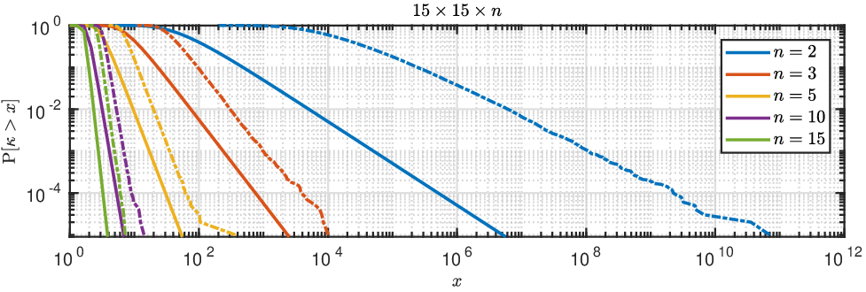
Figure 3.1. The empirical complementary cumulative distribution function of the condition number for rank-1515 tensors of size 15×15×n15\times 15\times n is shown in dashed lines. The corresponding solid lines show the lower bound from Theorem 1.4. The tensors 𝒜=∑𝒾=115𝐚𝒾⊗𝐛𝒾⊗𝐜𝒾\mathpzc{A}=\sum_{i=1}^{15}\mathbf{a}_{i}\otimes\mathbf{b}_{i}\otimes\mathbf{c}_{i} were generated by randomly sampling factor matrices A∈ℝ15×15A\in\mathbb{R}^{15\times 15}, B∈ℝ15×15B\in\mathbb{R}^{15\times 15} and C∈ℝn×15C\in\mathbb{R}^{n\times 15}, as indicated.

Theorem 1.4 is illustrated in Figure 3.1 for 15×15×n15\times 15\times n tensors of rank 1515 for n=2,3,5,10,15n=2,3,5,10,15. Every solid line represents a limiting complementary cumulative distribution function (ccdf) limr→∞Tr,α\lim_{r\to\infty}T_{r,\alpha} from Theorem 1.4, which provide asymptotic lower bounds on the ccdfs of the condition numbers of random rank-rr CPDs. The dashed lines in Figure 3.1 show the empirical ccdfs of the condition number based on two different Monte Carlo experiments.

In the first set of experiments, visualized in Figure 3.1(A), we generated 10510^{5} random rank-15 tensors 𝒜=∑𝒾=115𝐚𝒾⊗𝐛𝒾⊗𝐜𝒾\mathpzc{A}=\sum_{i=1}^{15}\mathbf{a}_{i}\otimes\mathbf{b}_{i}\otimes\mathbf{c}_{i} by independently sampling the entries of the factor matrices A=[𝐚i]∈ℝ15×15A=[\mathbf{a}_{i}]\in\mathbb{R}^{15\times 15}, B=[𝐛i]∈ℝ15×15B=[\mathbf{b}_{i}]\in\mathbb{R}^{15\times 15} and C=[𝐜i]∈ℝn×15C=[\mathbf{c}_{i}]\in\mathbb{R}^{n\times 15} from a standard normal distribution. It is observed that the limiting distribution of Theorem 1.4 seems to approximate the shape of the distribution of the condition numbers reasonably well. However, the lower bound seems rather weak for n=2n=2. One of the main observations, which is also evident from the formula of the limiting distribution, is that as nn increases the probability of sampling tensors with a high condition number decreases. As is evident from the empirical ccdf in Figure 3.1(A), n=2n=2 admits the worst distribution by far: there is a 10%10\% probability of sampling a condition number greater than 10510^{5}, and still a 0.1%0.1\% chance to encounter a condition number greater than 10810^{8}. On the other hand, for n=15n=15, all sampled tensors had a condition number less than 1010.

In the second set of experiments, shown in Figure 3.1(B), we generated 10510^{5} random rank-1515 tensors of size 15×15×n15\times 15\times n in a different way in order to illustrate the quality of the lower bound in Theorem 1.4. This time, after sampling the factor matrices (A,B,C)(A,B,C) as above, we perform Gram–Schmidt orthogonalization of AA and BB. As can be seen in Figure 3.1(B), the empirical ccdfs here are close to the corresponding limiting distributions.

We had one additional reason to treat Theorem 1.4 first: on a fundamental level, a PBA solves the TDP for n1×n2×n3n_{1}\times n_{2}\times n_{3} tensors by transforming it into a TDP for n1×n2×2n_{1}\times n_{2}\times 2 tensors. The above experiments clearly show that the latter problem has a much worse distribution of condition numbers than the original problem. In other words, from the viewpoint of sensitivity, PBAs try to solve an easy problem via the solution of a significantly more difficult problem. This approach is nearly guaranteed to end in instability.

4. The manifold of rr-nice tensors

While the instability of PBAs is already plausible from Figure 3.1, proving Theorem 1.2 is substantially more complicated. In order to prove it, we should first formalize what we mean by “solving a TDP.” This problem is rife with subtleties.

For example, what should the solution of a TDP be if the input tensor 𝒜\mathpzc{A} is the generic rank-1111 tensor in ℂ11×6×3\mathbb{C}^{11\times 6\times 3}? This tensor has 352,716352,716 isolated CPDs [24]. Computing all of them seems computationally infeasible. Nevertheless, all of them are well-behaved because each one of these will vary smoothly in a small open neighborhood of 𝒜\mathpzc{A} in ℂ11×6×3\mathbb{C}^{11\times 6\times 3}. On the other hand, the generic rank-66 tensor of multilinear rank (4,4,4)(4,4,4) ℬ\mathpzc{B} in ℂ6×6×6\mathbb{C}^{6\times 6\times 6} behaves erratically. It has 22 isolated decompositions [11, Theorem 1.3], but a generic rank-66 tensor close to ℬ\mathpzc{B} has only one decomposition that can be moved around continuously such that its limit is a decomposition of ℬ\mathpzc{B}. This process works for both of ℬ\mathpzc{B}’s decompositions, because the rank-66 tensors have two smooth folds meeting in ℬ\mathpzc{B} [12, Example 4.2]. What should an algorithm compute in this case?

For an rr-identifiable tensor 𝒜\mathpzc{A} there is an unambiguous answer to the above question. Namely, the solution is the unique set of rank-11 tensors {𝒜1,…,𝒜𝓇}\{\mathpzc{A}_{1},\ldots,\mathpzc{A}_{r}\} whose sum is 𝒜\mathpzc{A}. The goal of this section is to carefully define a tensor decomposition map τr;n1,…,nd\tau_{r;n_{1},\ldots,n_{d}} in Definition 4.8 whose computation solves the TDP for a subset of rank-rr tensors. The domain where the smooth function τr;n1,…,nd\tau_{r;n_{1},\ldots,n_{d}} is well defined deserves its own definition, Definition 4.1 below; we call it the manifold of rr-nice tensors 𝒩⊂σr\mathcal{N}\subset\sigma_{r}. In Proposition 4.7 we prove that 𝒩\mathcal{N} is a Zariski open dense subset of the set of rank-rr tensors, so that “almost all tensors are rr-nice.”

Before defining 𝒩\mathcal{N}, we first need the following two standard definitions. If for a collection of rr vectors 𝐩1,…,𝐩r∈ℝn\mathbf{p}_{1},\ldots,\mathbf{p}_{r}\in\mathbb{R}^{n} every subset of min⁡{r,n}\min\{r,n\} many vectors is linearly independent, then the vectors are said to lie in general linear position (GLP). We say that a collection of rr rank-11 tensors {𝐚i1⊗⋯⊗𝐚id}i\{\mathbf{a}_{i}^{1}\otimes\cdots\otimes\mathbf{a}_{i}^{d}\}_{i} is in super general linear position (SGLP) if for every 1≤s≤d1\leq s\leq d and every 𝐡⊂{1,…,d}\mathbf{h}\subset\{1,\ldots,d\} with |𝐡|=s|\mathbf{h}|=s, the set {𝐚ih1⊗⋯⊗𝐚ihs}i\{\mathbf{a}_{i}^{h_{1}}\otimes\cdots\otimes\mathbf{a}_{i}^{h_{s}}\}_{i} is in GLP.

Definition 4.1 (rr-nice tensors).

Recall from 2.3 the definition of rank-rr tensors σr\sigma_{r} and its closure σr¯\overline{\sigma_{r}}. Then, ℳr;n1,…,nd⊂𝒮n1,…,nd×r\mathcal{M}_{r;n_{1},\ldots,n_{d}}\subset\mathcal{S}_{n_{1},\ldots,n_{d}}^{\times r} is defined to be the set containing all the rank-11 tuples 𝔞=(𝒜1,…,𝒜𝓇)\mathfrak{a}=(\mathpzc{A}_{1},\ldots,\mathpzc{A}_{r}) satisfying the following properties:

  1. (i)

    Φr​(𝔞)\Phi_{r}(\mathfrak{a}) is a smooth point of σr¯\overline{\sigma_{r}},

  2. (ii)

    Φr​(𝔞)\Phi_{r}(\mathfrak{a}) is rr-identifiable, and, thus, has rank equal to rr,

  3. (iii)

    𝔞\mathfrak{a} has finite condition number,

  4. (iv)

    𝔞\mathfrak{a} is in SGLP, and

  5. (v)

    for all ii the (1,1,…,1)(1,1,\ldots,1)-entry of 𝒜𝒾\mathpzc{A}_{i} is not equal to zero.

The rr-nice tensors 𝒩r;n1,…,nd\mathcal{N}_{r;n_{1},\ldots,n_{d}} are defined to be the image of ℳr;n1,…,nd\mathcal{M}_{r;n_{1},\ldots,n_{d}} under the addition map Φr\Phi_{r} from 2.2:

𝒩r;n1,…,nd:=Φr​(ℳr;n1,…,nd).\mathcal{N}_{r;n_{1},\ldots,n_{d}}:=\Phi_{r}(\mathcal{M}_{r;n_{1},\ldots,n_{d}}).

If it is clear from the context we drop the subscript from both ℳr;n1,…,nd\mathcal{M}_{r;n_{1},\ldots,n_{d}} and 𝒩r;n1,…,nd\mathcal{N}_{r;n_{1},\ldots,n_{d}} and simply write ℳ\mathcal{M} and 𝒩\mathcal{N}.

Remark 4.2.

The reason for the last requirement, (v), is that under this restriction we can define a parametrization of rank-11 tensors that is a diffeomorphism; see the next subsection for details.

4.1. Elementary results

Before proceeding, we need a few elementary results related to the differential geometry of CPDs, which we did not find in the literature.

The rank-11 tensors in ℝn1×⋯×nd\mathbb{R}^{n_{1}\times\cdots\times n_{d}}, i.e., 𝒮={𝐚1⊗⋯⊗𝐚d|𝐚k∈ℝnk}∖{0},\mathcal{S}=\{\mathbf{a}_{1}\otimes\cdots\otimes\mathbf{a}_{d}\;|\;\mathbf{a}_{k}\in\mathbb{R}^{n_{k}}\}\setminus\{0\}, form the affine cone over a smooth projective variety (see, e.g., [31]) and, hence, 𝒮\mathcal{S} is an analytic submanifold of ℝn1×⋯×nd\mathbb{R}^{n_{1}\times\cdots\times n_{d}}. Its dimension is 1+∑k=1d(nk−1)1+\sum_{k=1}^{d}(n_{k}-1) [31]. The map22 2 The following items are most naturally considered in projective space, but in order to avoid as much technicalities as is feasible we prefer to present the results concretely as subspaces of Euclidean spaces.

Ψn1,…,nd:ℝ∖{0}×𝕊(ℝn1)×⋯×𝕊(ℝnd)→𝒮,(λ,𝐮1,…,𝐮d)↦λ𝐮1⊗⋯⊗𝐮d\Psi_{n_{1},\ldots,n_{d}}:\mathbb{R}\setminus\{0\}\times\mathbb{S}(\mathbb{R}^{n_{1}})\times\cdots\times\mathbb{S}(\mathbb{R}^{n_{d}})\to\mathcal{S},\;(\lambda,\mathbf{u}_{1},\ldots,\mathbf{u}_{d})\mapsto\lambda\mathbf{u}_{1}\otimes\cdots\otimes\mathbf{u}_{d}

is a surjective local diffeomorphism: every point in the domain has an open neighborhood such that Ψn1,…,nd\Psi_{n_{1},\ldots,n_{d}} restricted to this neighborhood is an open, smooth (C∞C^{\infty}), bijective map with smooth inverse [32, p. 79]. Indeed, it can be verified that the derivative is injective at every point; see, e.g., [4, Section 5.1]. Note that the fiber of Ψn1,…,nd\Psi_{n_{1},\ldots,n_{d}} at λ𝐮1⊗⋯⊗𝐮d\lambda\mathbf{u}_{1}\otimes\cdots\otimes\mathbf{u}_{d} is exactly the set {(ω0λ,ω1𝐮1,…,ωd𝐮d)|ω0⋯ωd=1,ωi∈{−1,1}}\{(\omega_{0}\lambda,\omega_{1}\mathbf{u}_{1},\ldots,\omega_{d}\mathbf{u}_{d})\;|\;\omega_{0}\cdots\omega_{d}=1,\omega_{i}\in\{-1,1\}\}, which has 2d2^{d} elements. Moreover, Ψn1,…,nd\Psi_{n_{1},\ldots,n_{d}} is a proper map so that it is a 2d2^{d}-sheeted smooth covering map [32, p. 91–95].

Let 𝕊+​(ℝn)={𝐮∈𝕊⁡(ℝn)|u1>0}\mathbb{S}^{+}(\mathbb{R}^{n})=\{\mathbf{u}\in\mathbb{S}(\mathbb{R}^{n})\;|\;u_{1}>0\} be the “upper” half of the unit sphere; it is a submanifold in the subspace topology on ℝn\mathbb{R}^{n}. Let us define the following restriction of Ψ\Psi:

(4.1) Ψn1,…,nd∗:ℝ∖{0}×𝕊+(ℝn1)×⋯×𝕊+(ℝnd)→𝒮,(λ,𝐮1,…,𝐮d)↦λ𝐮1⊗⋯⊗𝐮d.\Psi^{*}_{n_{1},\ldots,n_{d}}:\mathbb{R}\setminus\{0\}\times\mathbb{S}^{+}(\mathbb{R}^{n_{1}})\times\cdots\times\mathbb{S}^{+}(\mathbb{R}^{n_{d}})\to\mathcal{S},\;(\lambda,\mathbf{u}_{1},\ldots,\mathbf{u}_{d})\mapsto\lambda\mathbf{u}_{1}\otimes\cdots\otimes\mathbf{u}_{d}.

It follows from the foregoing that Ψn1,…,nr∗\Psi^{*}_{n_{1},\ldots,n_{r}} is a bijective local diffeomorphism onto its image, so it is a (global) diffeomorphism onto its image. Let 𝒮n1,…,nr∗\mathcal{S}^{*}_{n_{1},\ldots,n_{r}} be the image of Ψn1,…,nr∗\Psi^{*}_{n_{1},\ldots,n_{r}}:

(4.2) 𝒮n1,…,nr∗:=Ψn1,…,nr∗(ℝ∖{0}×𝕊+(ℝn1)×⋯×𝕊+(ℝnd)).\mathcal{S}^{*}_{n_{1},\ldots,n_{r}}:=\Psi^{*}_{n_{1},\ldots,n_{r}}(\mathbb{R}\setminus\{0\}\times\mathbb{S}^{+}(\mathbb{R}^{n_{1}})\times\cdots\times\mathbb{S}^{+}(\mathbb{R}^{n_{d}})).

When it is clear from the context we drop the subscripts from Ψn1,…,nd\Psi_{n_{1},\ldots,n_{d}}, Ψn1,…,nd∗\Psi_{n_{1},\ldots,n_{d}}^{*} and 𝒮n1,…,nd∗\mathcal{S}_{n_{1},\ldots,n_{d}}^{*}. The foregoing explains part (v) in Definition 4.1: we wish to work with a parametrization of 𝒮\mathcal{S} that is a diffeomorphism, so we restrict ourselves to 𝒮∗\mathcal{S}^{*} and use Ψ∗\Psi^{*}. We will show in the proof of Proposition 4.5 that 𝒮∗\mathcal{S}^{*} is open in the Zariski topology and, hence, open and dense in the Euclidean topology.

Finally, we consider the subset Sr;n⊂(𝕊+​(ℝn))×rS_{r;n}\subset(\mathbb{S}^{+}(\mathbb{R}^{n}))^{\times r} defined as

(4.3) Sr;n={(s1,…,sr)∈(𝕊+​(ℝn))×r∣[s1,…,sr]∈ℝn×r​ has full rank}.S_{r;n}=\{(s_{1},\ldots,s_{r})\in(\mathbb{S}^{+}(\mathbb{R}^{n}))^{\times r}\mid[s_{1},\ldots,s_{r}]\in\mathbb{R}^{n\times r}\text{ has full rank}\}.

Note that Sr;nS_{r;n} is an open submanifold, because the locus of points not satisfying the rank condition is closed in the Zariski topology. We also have the following result.

Lemma 4.3.

Let 𝔖r\mathfrak{S}_{r} be the symmetric group on rr elements. Then, S^r;n:=Sr;n/𝔖r\widehat{S}_{r;n}:=S_{r;n}/\mathfrak{S}_{r} is a manifold. Moreover, the projection π:Sr;n→S^r;n,(x1,…,xr)↦{x1,…,xr}\pi:S_{r;n}\to\widehat{S}_{r;n},(x_{1},\ldots,x_{r})\mapsto\{x_{1},\ldots,x_{r}\} is a local diffeomorphism.

Proof.

𝔖r\mathfrak{S}_{r} is a discrete Lie group acting smoothly [32, Example 7.22(e)]. The group action is also free because S∈Sr;nS\in S_{r;n} can be a fixed point of some permutation only if si,sj∈Ss_{i},s_{j}\in S with i≠ji\neq j are equal. It can be verified that the conditions in [32, Lemma 21.11] hold, so that the action is proper. The result follows by the quotient manifold theorem [32, Theorem 21.10]. ∎

4.2. Differential geometry of rr-nice tensors

Recall that a Segre manifold 𝒮⊂ℝn1×⋯×nd\mathcal{S}\subset\mathbb{R}^{n_{1}\times\cdots\times n_{d}} is said to be generically rr-identifiable if all tensors in a Zariski-open subset of σr¯\overline{\sigma_{r}} are identifiable; see [12, 13] for the state of the art. In the context of PBAs, the following standard result suffices.

Lemma 4.4.

Let n1≥n2≥⋯≥nd≥2n_{1}\geq n_{2}\geq\cdots\geq n_{d}\geq 2. If r≤n2r\leq n_{2}, then 𝒮n1,…,nd\mathcal{S}_{n_{1},\ldots,n_{d}} is generically rr-identifiable.

Proof.

This is follows, for example, from the effectiveness of Kruskal’s criterion; see [13]. ∎

Next, we prove an important property of the set ℳr;n1,…,nd\mathcal{M}_{r;n_{1},\ldots,n_{d}} from Definition 4.1.

Proposition 4.5.

Let 𝒮n1,…,nd\mathcal{S}_{n_{1},\ldots,n_{d}} be generically rr-identifiable. Then, ℳr;n1,…,nd\mathcal{M}_{r;n_{1},\ldots,n_{d}} is a Zariski-open submanifold of 𝒮n1,…,nd×r\mathcal{S}_{n_{1},\ldots,n_{d}}^{\times r}.

Proof.

Let 𝒮=𝒮n1,…,nd\mathcal{S}=\mathcal{S}_{n_{1},\ldots,n_{d}} and ℳ=ℳr;n1,…,nd\mathcal{M}=\mathcal{M}_{r;n_{1},\ldots,n_{d}} for brevity. We show that the set of tuples not satisfying either of the conditions in Definition 4.1 is contained in a union of five Zariski-closed subsets of ℳ\mathcal{M}; these subsets are denoted by ℬ(i),ℬ(ii),ℬ(iii),ℬ(iv)\mathcal{B}_{\mathrm{(i)}},\mathcal{B}_{\mathrm{(ii)}},\mathcal{B}_{\mathrm{(iii)}},\mathcal{B}_{\mathrm{(iv)}} and ℬ(v)\mathcal{B}_{\mathrm{(v)}}. Taking

ℳ=𝒮×r\(ℬ(i)∪ℬ(ii)∪ℬ(iii)∪ℬ(iv)∪ℬ(v))\mathcal{M}=\mathcal{S}^{\times r}\backslash\left(\mathcal{B}_{\mathrm{(i)}}\cup\mathcal{B}_{\mathrm{(ii)}}\cup\mathcal{B}_{\mathrm{(iii)}}\cup\mathcal{B}_{\mathrm{(iv)}}\cup\mathcal{B}_{\mathrm{(v)}}\right)

would then prove the assertion.

Recall that generic rr-identifiability implies nondefectivity of σr\sigma_{r}; see [31, Chapter 5, specifically Corollary 5.3.1.3]. Hence, dimσr=dimσr¯=dim𝒮×r=r​dim𝒮\dim\sigma_{r}=\dim\overline{\sigma_{r}}=\dim\mathcal{S}^{\times r}=r\dim\mathcal{S}. The subvariety Σ⊂σr¯\Sigma\subset\overline{\sigma_{r}} of singular points is proper and closed in the Zariski topology by definition [23]. This means that in addition to the polynomials that vanish on the ℝ\mathbb{R}-variety σr¯\overline{\sigma_{r}}, there are k≥1k\geq 1 additional nontrivial polynomial equations with coefficients over ℝ\mathbb{R} such that f1​(y)=⋯=fk​(y)=0f_{1}(y)=\cdots=f_{k}(y)=0 for all y∈Σy\in\Sigma. If yy has a preimage x∈𝒮×rx\in\mathcal{S}^{\times r} under Φr\Phi_{r}, then f1​(Φr​(x))=⋯=fk​(Φr​(x))=0f_{1}(\Phi_{r}(x))=\cdots=f_{k}(\Phi_{r}(x))=0. Hence, the locus ℬ(i)\mathcal{B}_{\mathrm{(i)}} of decompositions not satisfying condition (i) in Definition 4.1, which map into the singular locus Σ\Sigma under Φr\Phi_{r} is a Zariski-closed set. It is also a proper subset, because otherwise Φr​(𝒮×r)=σr⊂Σ\Phi_{r}(\mathcal{S}^{\times r})=\sigma_{r}\subset\Sigma, which is a contradiction as dimΣ<dimσr¯=dimσr\dim\Sigma<\dim\overline{\sigma_{r}}=\dim\sigma_{r}.

The set of tensors in σr¯\overline{\sigma_{r}} with several decompositions is closed in the Zariski topology by assumption. We can apply the same argument as in the previous paragraph to conclude that the variety of decompositions ℬ(ii)⊂𝒮×r\mathcal{B}_{\mathrm{(ii)}}\subset\mathcal{S}^{\times r} that map to points of σr¯\overline{\sigma_{r}} that are not rr-identifiable is a proper Zariski closed subset in 𝒮×r\mathcal{S}^{\times r}.

The subset ℬ(iii)⊂𝒮×r\mathcal{B}_{\mathrm{(iii)}}\subset\mathcal{S}^{\times r} of decompositions with condition number ∞\infty, is contained in a Zariski-closed set if the rr-secant variety σr¯\overline{\sigma_{r}} is nondefective by [6, Lemma 5.3].

The set of points ℬ(iv)⊂𝒮×r\mathcal{B}_{\mathrm{(iv)}}\subset\mathcal{S}^{\times r} not satisfying (iv) is Zariski-closed by [13, Lemma 4.4].

For the last point, observe that condition (v) of Definition 4.1 is equivalent to p∈(𝒮∗)×rp\in(\mathcal{S}^{*})^{\times r}. By definition of 𝒮∗\mathcal{S}^{*} in 4.2, the set of points in 𝒮∖𝒮∗\mathcal{S}\setminus\mathcal{S}^{*} is the intersection of 𝒮\mathcal{S} with the union of the following linear varieties: Lk=ℝn1⊗⋯⊗ℝnk−1⊗ℝnk/⟨𝐞1⟩⊗ℝnk+1⊗⋯⊗ℝnd,L_{k}=\mathbb{R}^{n_{1}}\otimes\cdots\otimes\mathbb{R}^{n_{k-1}}\otimes\mathbb{R}^{n_{k}}/\langle\mathbf{e}_{1}\rangle\otimes\mathbb{R}^{n_{k+1}}\otimes\cdots\otimes\mathbb{R}^{n_{d}}, where ℝnk/⟨𝐞1⟩=⟨𝐞2,…,𝐞nk⟩\mathbb{R}^{n_{k}}/\langle\mathbf{e}_{1}\rangle=\langle\mathbf{e}_{2},\ldots,\mathbf{e}_{n_{k}}\rangle and 𝐞i\mathbf{e}_{i} is the iith standard basis vector of ℝnk\mathbb{R}^{n_{k}}. In fact,

𝒮∖𝒮∗=𝒮∩(⋃k=1dLk)=⋃k=1d(𝒮∩Lk)≃⋃k=1d𝒮n1,…,nk−1,nk−1,nk+1,…,nd,{\mathcal{S}\setminus\mathcal{S}^{*}=\mathcal{S}\cap\left(\bigcup_{k=1}^{d}L_{k}\right)=\bigcup_{k=1}^{d}(\mathcal{S}\cap L_{k})\simeq\bigcup_{k=1}^{d}\mathcal{S}_{n_{1},\ldots,n_{k-1},n_{k}-1,n_{k+1},\ldots,n_{d}},}

which is thus a Zariski-closed set because dim𝒮n1,…,nk−1,nk−1,nk+1,…,nd<dim𝒮\dim\mathcal{S}_{n_{1},\ldots,n_{k-1},n_{k}-1,n_{k+1},\ldots,n_{d}}<\dim\mathcal{S}. Therefore, taking ℬ(v)=⋃i=1r𝒮×(i−1)×(𝒮∖𝒮∗)×𝒮×(r−i)\mathcal{B}_{\mathrm{(v)}}=\bigcup_{i=1}^{r}\mathcal{S}^{\times(i-1)}\times(\mathcal{S}\setminus\mathcal{S}^{*})\times\mathcal{S}^{\times(r-i)} yields the Zariski-closed variety of points not satisfying (v). This concludes the proof. ∎

The definition of ℳr;n1,…,nd\mathcal{M}_{r;n_{1},\ldots,n_{d}} is nice, because the addition map Φr\Phi_{r} from 2.2 restricted to ℳr;n1,…,nd\mathcal{M}_{r;n_{1},\ldots,n_{d}} is a local diffeomorphism. However, we wish to work with global diffeomorphisms and therefore need the following proposition.

Proposition 4.6.

If 𝒮n1,…,nd\mathcal{S}_{n_{1},\ldots,n_{d}} is generically rr-identifiable, then ℳ^r;n1,…,nd=ℳr;n1,…,nd/𝔖r\widehat{\mathcal{M}}_{r;n_{1},\ldots,n_{d}}=\mathcal{M}_{r;n_{1},\ldots,n_{d}}/\mathfrak{S}_{r} is a manifold. Moreover, the projection π^:ℳr;n1,…,nd→ℳ^r;n1,…,nd,(𝒜1,…,𝒜𝓇)↦{𝒜1,…,𝒜𝓇}\widehat{\pi}:\mathcal{M}_{r;n_{1},\ldots,n_{d}}\to\widehat{\mathcal{M}}_{r;n_{1},\ldots,n_{d}},(\mathpzc{A}_{1},\ldots,\mathpzc{A}_{r})\mapsto\{\mathpzc{A}_{1},\ldots,\mathpzc{A}_{r}\} is a local diffeomorphism.

Proof.

Combine the proof of Lemma 4.3 with the fact that rr-identifiability implies that the rank-1 tensors in a decomposition (𝒜1,…,𝒜𝓇)∈ℳ𝓇;𝓃1,…,𝓃𝒹(\mathpzc{A}_{1},\ldots,\mathpzc{A}_{r})\in\mathcal{M}_{r;n_{1},\ldots,n_{d}} are pairwise distinct. ∎

It is clear that the addition map Φr\Phi_{r} is constant on 𝔖r\mathfrak{S}_{r}-orbits in ℳr;n1,…,nd\mathcal{M}_{r;n_{1},\ldots,n_{d}}. Therefore, Φr\Phi_{r} is well defined on ℳ^r;n1,…,nd\widehat{\mathcal{M}}_{r;n_{1},\ldots,n_{d}}. Now, we have the following crucial result.

Proposition 4.7.

Let 𝒩rn1,…,nd⊂σr\mathcal{N}_{r}^{n_{1},\ldots,n_{d}}\subset\sigma_{r} be the set of rr-nice tensors. If 𝒮n1,…,nd\mathcal{S}_{n_{1},\ldots,n_{d}} is generically rr-identifiable, then

Φr:ℳ^r;n1,…,nd→𝒩rn1,…,nd,{𝒜1,…,𝒜𝓇}↦𝒜1+⋯+𝒜𝓇\Phi_{r}:\widehat{\mathcal{M}}_{r;n_{1},\ldots,n_{d}}\to\mathcal{N}_{r}^{n_{1},\ldots,n_{d}},\;\{\mathpzc{A}_{1},\ldots,\mathpzc{A}_{r}\}\mapsto\mathpzc{A}_{1}+\cdots+\mathpzc{A}_{r}

is a diffeomorphism. Moreover, 𝒩r;n1,…,nd\mathcal{N}_{r;n_{1},\ldots,n_{d}} is an open dense submanifold of σr\sigma_{r}.

Proof.

As before, for brevity, we drop all subscripts. Let 𝔞=(𝒜1,…,𝒜𝓇)∈ℳ\mathfrak{a}=(\mathpzc{A}_{1},\ldots,\mathpzc{A}_{r})\in\mathcal{M}. By definition, 𝔞\mathfrak{a} has a finite condition number. This means, by [4, Theorem 1.1], that the derivative of Φr\Phi_{r} at 𝔞\mathfrak{a} is injective. Hence, Φr\Phi_{r} is a smooth immersion [32, p. 78]. By the generic rr-identifiability assumption, it follows that the rr-secant variety σr¯\overline{\sigma_{r}} is not defective so that dimσr¯=r​dim𝒮\dim\overline{\sigma_{r}}=r\dim\mathcal{S}. Moreover, by Proposition 4.5, we have r​dim𝒮=dimℳr;n1,…,ndr\dim\mathcal{S}=\dim\mathcal{M}_{r;n_{1},\ldots,n_{d}} and, by construction, we have dimℳr;n1,…,nd=dimℳ^r;n1,…,nd\dim\mathcal{M}_{r;n_{1},\ldots,n_{d}}=\dim\widehat{\mathcal{M}}_{r;n_{1},\ldots,n_{d}}. As Φr\Phi_{r} is injective by generic rr-identifiability and by having taken the particular quotient in Proposition 4.6, then [32, Proposition 4.22(d)] entails that Φr\Phi_{r} is a smooth embedding. The first conclusion follows by [32, Proposition 5.2].

The foregoing already shows that 𝒩r;n1,…,nd⊂σr\mathcal{N}_{r;n_{1},\ldots,n_{d}}\subset\sigma_{r} is open. We show that it is dense. Let 𝒜∈σ𝓇∖𝒩𝓇;𝓃1,…,𝓃𝒹\mathpzc{A}\in\sigma_{r}\setminus\mathcal{N}_{r;n_{1},\ldots,n_{d}} with decomposition 𝒜=Φ𝓇​(𝔞)=𝒜1+⋯+𝒜𝓇\mathpzc{A}=\Phi_{r}(\mathfrak{a})=\mathpzc{A}_{1}+\cdots+\mathpzc{A}_{r}. By Proposition 4.5, there exist a sequence

(𝒜1(𝒿),…,𝒜𝓇(𝒿))∈ℳ𝓇;𝓃1,…,𝓃𝒹​ such that ​lim𝒿→∞(𝒜1(𝒿),…,𝒜𝓇(𝒿))→(𝒜1,…,𝒜𝓇).(\mathpzc{A}_{1}^{(j)},\ldots,\mathpzc{A}_{r}^{(j)})\in\mathcal{M}_{r;n_{1},\ldots,n_{d}}\text{ such that }\lim_{j\to\infty}(\mathpzc{A}_{1}^{(j)},\ldots,\mathpzc{A}_{r}^{(j)})\to(\mathpzc{A}_{1},\ldots,\mathpzc{A}_{r}).

Note that this is convergence in the usual Euclidean topology that ℳr;n1,…,nd\mathcal{M}_{r;n_{1},\ldots,n_{d}} inherits from the ambient space (ℝn1×⋯×nd)×r(\mathbb{R}^{n_{1}\times\cdots\times n_{d}})^{\times r}. Consequently, the components also converge individually: limj→∞𝒜𝒾(𝒿)→𝒜𝒾\lim_{j\to\infty}\mathpzc{A}_{i}^{(j)}\to\mathpzc{A}_{i}, i=1,…,r.i=1,\ldots,r. The result follows from the fact that adding the above convergent sequences results in a convergent sequence in 𝒩r;n1,…,nd\mathcal{N}_{r;n_{1},\ldots,n_{d}} with limit 𝒜\mathpzc{A}. Hence, 𝒜∈𝒩𝓇;𝓃1,…,𝓃𝒹¯\mathpzc{A}\in\overline{\mathcal{N}_{r;n_{1},\ldots,n_{d}}} so that 𝒩r;n1,…,nd\mathcal{N}_{r;n_{1},\ldots,n_{d}} is dense in σr\sigma_{r}, concluding the proof. ∎

From Proposition 4.7, Φr\Phi_{r} has an smooth inverse, which solves the TDP on 𝒩r;n1,…,nd⊂ℝn1×⋯×nd\mathcal{N}_{r;n_{1},\ldots,n_{d}}\subset\mathbb{R}^{n_{1}\times\cdots\times n_{d}}. We finally arrive at the goal of this section.

Definition 4.8.

The inverse of Φr\Phi_{r} on the manifold of rr-nice tensors is

τr;n1,…,nd:𝒩r;n1,…,nd→ℳ^r;n1,…,nd,𝒜1+⋯+𝒜𝓇↦{𝒜1,…,𝒜𝓇}.\tau_{r;n_{1},\ldots,n_{d}}:\mathcal{N}_{r;n_{1},\ldots,n_{d}}\to\widehat{\mathcal{M}}_{r;n_{1},\ldots,n_{d}},\;\mathpzc{A}_{1}+\cdots+\mathpzc{A}_{r}\mapsto\{\mathpzc{A}_{1},\ldots,\mathpzc{A}_{r}\}.

We call this mapping the tensor decomposition map.

Remark 4.9.

One way to interpret the construction in this section is that near 𝒜∈𝒩𝓇;𝓃1,…,𝓃𝒹\mathpzc{A}\in\mathcal{N}_{r;n_{1},\ldots,n_{d}} we locally have the identification τr;n1,…,nd=π^∘Φ𝔞−1,\tau_{r;n_{1},\ldots,n_{d}}=\widehat{\pi}\circ\Phi_{\mathfrak{a}}^{-1}, where 𝔞=(𝒜1,…,𝒜𝓇)\mathfrak{a}=(\mathpzc{A}_{1},\ldots,\mathpzc{A}_{r}) is any ordered rr-nice decomposition of 𝒜\mathpzc{A}, Φ𝔞−1\Phi_{\mathfrak{a}}^{-1} is the local inverse in 1.2, and π^\widehat{\pi} is as in Proposition 4.6.

4.3. Implications for the condition number

Let 𝔞=(𝒜1,…,𝒜𝓇)\mathfrak{a}=(\mathpzc{A}_{1},\ldots,\mathpzc{A}_{r}) be any ordered rr-nice decomposition in ℳr;n1,…,nd\mathcal{M}_{r;n_{1},\ldots,n_{d}}. For the rr-nice tensor 𝒜=𝒜1+⋯+𝒜𝓇∈𝒩𝓇;𝓃1,…,𝓃𝒹\mathpzc{A}=\mathpzc{A}_{1}+\cdots+\mathpzc{A}_{r}\in\mathcal{N}_{r;n_{1},\ldots,n_{d}}, we will relate the condition number κ​[τr;n1,…,nd]​(𝒜)\kappa[\tau_{r;n_{1},\ldots,n_{d}}](\mathpzc{A}), as in 2.4, to the condition number of the CPD κ⁡(𝒜1,…,𝒜𝓇)\kappa(\mathpzc{A}_{1},\ldots,\mathpzc{A}_{r}) from [4]. We have the following result.

Lemma 4.10.

Let us choose the Riemannian metrics on 𝒩r;n1,…,nd\mathcal{N}_{r;n_{1},\ldots,n_{d}} and ℳr;n1,…,nd\mathcal{M}_{r;n_{1},\ldots,n_{d}} inherited from their respective ambient spaces. Then, the mapping π^\widehat{\pi} from Proposition 4.6 induces a natural Riemannian metric on ℳ^r;n1,…,nd\widehat{\mathcal{M}}_{r;n_{1},\ldots,n_{d}} with the following properties:

  1. (1)

    π^\widehat{\pi} is a local isometry;

  2. (2)

    for all 𝒜=𝒜1+⋯+𝒜𝓇∈𝒩𝓇;𝓃1,…,𝓃𝒹\mathpzc{A}=\mathpzc{A}_{1}+\cdots+\mathpzc{A}_{r}\in\mathcal{N}_{r;n_{1},\ldots,n_{d}}, we have κ⁡(𝒜1,…,𝒜𝓇)=κ⁡[τ𝓇;𝓃1,…,𝓃𝒹]​(𝒜)\kappa(\mathpzc{A}_{1},\ldots,\mathpzc{A}_{r})=\kappa[\tau_{r;n_{1},\ldots,n_{d}}](\mathpzc{A}); and

  3. (3)

    for any {𝒜1,…,𝒜𝓇},{ℬ1,…,ℬ𝓇}∈ℳ^\{\mathpzc{A}_{1},\ldots,\mathpzc{A}_{r}\},\{\mathpzc{B}_{1},\ldots,\mathpzc{B}_{r}\}\in\widehat{\mathcal{M}} we have

    distℳ^​({𝒜1,…,𝒜𝓇},{ℬ1,…,ℬ𝓇})=minπ∈𝔖𝓇⁡(distℳ​((𝒜1,…,𝒜𝓇),π⁡(ℬ1,…,ℬ𝓇))).\mathrm{dist}_{\widehat{\mathcal{M}}}(\{\mathpzc{A}_{1},\ldots,\mathpzc{A}_{r}\},\{\mathpzc{B}_{1},\ldots,\mathpzc{B}_{r}\})=\min_{\pi\in\mathfrak{S}_{r}}\left(\mathrm{dist}_{\mathcal{M}}((\mathpzc{A}_{1},\ldots,\mathpzc{A}_{r}),\pi(\mathpzc{B}_{1},\ldots,\mathpzc{B}_{r}))\right).

Here, distℳ^\mathrm{dist}_{\widehat{\mathcal{M}}} and distℳ\mathrm{dist}_{\mathcal{M}} are the respective Riemannian distances.

Because of the equality of condition numbers in Lemma 4.10 and 1.2, we find that for every 𝔞=(𝒜1,…,𝒜𝓇)∈ℳ𝓇;𝓃1,…,𝓃𝒹\mathfrak{a}=(\mathpzc{A}_{1},\ldots,\mathpzc{A}_{r})\in\mathcal{M}_{r;n_{1},\ldots,n_{d}} we have

κ⁡[τ]​(𝒜)=limϵ→0supℬ∈σ𝓇‖𝒜−ℬ‖ℱ≤ϵdistℳ^​(τ⁡(𝒜),τ⁡(ℬ))‖𝒜−ℬ‖ℱ=limϵ→0supℬ∈σ𝓇‖𝒜−ℬ‖ℱ≤ϵminπ∈𝔖𝓇⁡‖Φ𝔞−1​(𝒜)−π∘Φ𝔞−1​(ℬ)‖ℱ‖𝒜−ℬ‖ℱ,\kappa[\tau](\mathpzc{A})=\lim_{\epsilon\to 0}\sup_{\begin{subarray}{c}\mathpzc{B}\in\sigma_{r}\\ \|\mathpzc{A}-\mathpzc{B}\|_{F}\leq\epsilon\end{subarray}}\frac{\mathrm{dist}_{\widehat{\mathcal{M}}}(\tau(\mathpzc{A}),\tau(\mathpzc{B}))}{\|\mathpzc{A}-\mathpzc{B}\|_{F}}=\lim_{\epsilon\to 0}\sup_{\begin{subarray}{c}\mathpzc{B}\in\sigma_{r}\\ \|\mathpzc{A}-\mathpzc{B}\|_{F}\leq\epsilon\end{subarray}}\min_{\pi\in\mathfrak{S}_{r}}\frac{\|\Phi_{\mathfrak{a}}^{-1}(\mathpzc{A})-\pi\circ\Phi_{\mathfrak{a}}^{-1}(\mathpzc{B})\|_{F}}{\|\mathpzc{A}-\mathpzc{B}\|_{F}},

where τ=τr;n1,…,nd\tau=\tau_{r;n_{1},\ldots,n_{d}} and the last equality follows from (3)(3) in Lemma 4.10. This above equality is very significant because it allows us to make sense of the distance between two unordered CPDs, i.e., sets of rank-11 tensors, {𝒜1,…,𝒜𝓇}\{\mathpzc{A}_{1},\ldots,\mathpzc{A}_{r}\} and {ℬ1,…,ℬ𝓇}\{\mathpzc{B}_{1},\ldots,\mathpzc{B}_{r}\}. As a consequence, we get an instance of the well-known rule of thumb in numerical analysis:

(4.4) minπ∈𝔖r⁡‖A−B​Pπ‖F⏟forward error≲κ​[τ]​(𝒜)⏟condition number⋅‖𝒜−ℬ‖ℱ⏟backward error\displaystyle\underbrace{\min_{\pi\in\mathfrak{S}_{r}}\|A-BP_{\pi}\|_{F}}_{\text{forward error}}\lesssim\underbrace{\kappa[\tau](\mathpzc{A})}_{\text{condition number}}\cdot\underbrace{\|\mathpzc{A}-\mathpzc{B}\|_{F}}_{\text{backward error}}

for nearby 𝒜=𝒜1+⋯+𝒜𝓇\mathpzc{A}=\mathpzc{A}_{1}+\cdots+\mathpzc{A}_{r} and ℬ=ℬ1+⋯+ℬ𝓇\mathpzc{B}=\mathpzc{B}_{1}+\cdots+\mathpzc{B}_{r}; herein, A=[𝒜𝒾]𝒾∈ℝ𝓃1⋯𝓃𝒹×𝓇A=[\mathpzc{A}_{i}]_{i}\in\mathbb{R}^{n_{1}\cdots n_{d}\times r} (resp. B=[ℬ𝒾]𝒾∈ℝ𝓃1⋯𝓃𝒹×𝓇B=[\mathpzc{B}_{i}]_{i}\in\mathbb{R}^{n_{1}\cdots n_{d}\times r}) is a matrix that contains the vectorized rank-11 tensors 𝒜𝒾\mathpzc{A}_{i} (resp. ℬ𝒾\mathpzc{B}_{i}) as columns, and PπP_{\pi} is the r×rr\times r permutation matrix representing the permutation π\pi. The notation ≲\lesssim indicates that the bound is asymptotically sharp for infinitesimal ‖𝒜−ℬ‖ℱ\|\mathpzc{A}-\mathpzc{B}\|_{F}.

5. Pencil-based algorithms for the CPD

We start by specifying a very general class of numerical algorithms to which the analysis in Section 6 applies. The construction may seem a bit abstract at first sight, so it is useful to keep in mind that the prototypical algorithm from the introduction is an example of a PBA.

As it suffices, in principle, to present a single input for which an algorithm is unstable, we can choose a well-behaved subset of rr-nice tensors 𝒩∗⊂𝒩r;n1,n2,n3⊂ℝn1×n2×n3\mathcal{N}^{*}\subset\mathcal{N}_{r;n_{1},n_{2},n_{3}}\subset\mathbb{R}^{n_{1}\times n_{2}\times n_{3}} (for the exact choice of 𝒩∗\mathcal{N}^{*} see Definition 5.1 below) and specify what a PBA should compute for such inputs. If the numerical instability already occurs on this subset, then it is also unstable on larger domains. We recall from Section 4 that by considering only rr-nice tensors 𝒩r;n1,n2,n3\mathcal{N}_{r;n_{1},n_{2},n_{3}}, the TDP consists of computing the action of the function τr;n1,n2,n3\tau_{r;n_{1},n_{2},n_{3}} from Definition 4.8. PBAs compute this map in a particular way, via the four transformations described below.

The input of a PBA is assumed to be the multidimensional array 𝒜∈ℝ𝓃1×𝓃2×𝓃3\mathpzc{A}\in\mathbb{R}^{n_{1}\times n_{2}\times n_{3}}. The first transformation is the multilinear multiplication ρQ\rho_{Q} that maps n1×n2×n3n_{1}\times n_{2}\times n_{3} tensors to format n1×n2×2n_{1}\times n_{2}\times 2 via the matrix Q∈ℝn3×2Q\in\mathbb{R}^{n_{3}\times 2} with orthonormal columns:

ρQ:ℝn1×n2×n3→ℝn1×n2×2,𝒜↦(ℐ𝓃1,ℐ𝓃2,𝒬𝒯)⋅𝒜.\rho_{Q}:\mathbb{R}^{n_{1}\times n_{2}\times n_{3}}\to\mathbb{R}^{n_{1}\times n_{2}\times 2},\;\mathpzc{A}\mapsto(I_{n_{1}},I_{n_{2}},Q^{T})\cdot\mathpzc{A}.

The second transformation, θ^\widehat{\theta}, computes the set of unit-norm columns of the first factor matrix AA of the CPD when restricted to 𝒩r;n1,n2,2\mathcal{N}_{r;n_{1},n_{2},2}:

θ^|𝒩r;n1,n2,2:𝒩r;n1,n2,2→S^r;n1,ℬ=∑𝒾=1𝓇𝐚𝒾⊗𝐛𝒾⊗𝐳𝒾↦{𝐚1,…,𝐚𝓇}.\widehat{\theta}|_{\mathcal{N}_{r;n_{1},n_{2},2}}:\mathcal{N}_{r;n_{1},n_{2},2}\to\widehat{S}_{r;n_{1}},\quad\mathpzc{B}=\sum_{i=1}^{r}\mathbf{a}_{i}\otimes\mathbf{b}_{i}\otimes{\mathbf{z}}_{i}\mapsto\{\mathbf{a}_{1},\ldots,\mathbf{a}_{r}\}.

Herein, S^r;n1=Sr;n1/𝔖r\widehat{S}_{r;n_{1}}=S_{r;n_{1}}/\mathfrak{S}_{r}, where Sr;n1S_{r;n_{1}} is as in 4.3. Note the curious definition of θ^\widehat{\theta} involving the restriction to 𝒩r;n1,n2,n3\mathcal{N}_{r;n_{1},n_{2},n_{3}}. The reason for this formulation is that a PBA will be executed using floating-point arithmetic. It is unlikely that the floating point representation fl⁡(ℬ)∈ℝ𝓃1×𝓃2×2\operatorname{fl}(\mathpzc{B})\in\mathbb{R}^{n_{1}\times n_{2}\times 2} is exactly in 𝒩r;n1,n2,2⊂ℝn1×n2×2\mathcal{N}_{r;n_{1},n_{2},2}\subset\mathbb{R}^{n_{1}\times n_{2}\times 2}, even when ℬ∈𝒩𝓇;𝓃1,𝓃2,2\mathpzc{B}\in\mathcal{N}_{r;n_{1},n_{2},2}. Therefore, a minimal additional demand is placed on θ^\widehat{\theta}: For every ℬ∈𝒩𝓇;𝓃1,𝓃2,2\mathpzc{B}\in\mathcal{N}_{r;n_{1},n_{2},2}, θ^\widehat{\theta} must be defined for fl⁡(ℬ)\operatorname{fl}(\mathpzc{B}).

The third transformation, υ\upsilon, when restricted to

ℛr;n1,n2,n3:={(𝒜,𝒜)∣𝒜=(𝐚1,…,𝐚𝓇)∈𝒮𝓇;𝓃1​ and ​𝒜=∑𝒾=1𝓇𝐚𝒾⊗𝐛𝒾⊗𝐜𝒾∈𝒩𝓇;𝓃1,𝓃2,𝓃3},\mathcal{R}_{r;n_{1},n_{2},n_{3}}:=\bigl\{(\mathpzc{A},A)\mid A=(\mathbf{a}_{1},\ldots,\mathbf{a}_{r})\in S_{r;n_{1}}\text{ and }\mathpzc{A}=\sum_{i=1}^{r}\mathbf{a}_{i}\otimes\mathbf{b}_{i}\otimes\mathbf{c}_{i}\in\mathcal{N}_{r;n_{1},n_{2},n_{3}}\bigr\},

essentially computes the Khatri–Rao product B⊙CB\odot C of the remaining factor matrices, namely

υ|ℛr;n1,n2,n3:ℛr;n1,n2,n3→𝒮n2,n3×r,(𝒜=∑𝒾=1𝓇𝐚𝒾⊗𝐛𝒾⊗𝐜𝒾,(𝐚1,…,𝐚𝓇))↦(𝐛1⊗𝐜1,…,𝐛𝓇⊗𝐜𝓇).\upsilon|_{\mathcal{R}_{r;n_{1},n_{2},n_{3}}}:\mathcal{R}_{r;n_{1},n_{2},n_{3}}\to\mathcal{S}_{n_{2},n_{3}}^{\times r},\;\Bigl(\mathpzc{A}=\sum_{i=1}^{r}\mathbf{a}_{i}\otimes\mathbf{b}_{i}\otimes\mathbf{c}_{i},(\mathbf{a}_{1},\ldots,\mathbf{a}_{r})\Bigr)\mapsto(\mathbf{b}_{1}\otimes\mathbf{c}_{1},\ldots,\mathbf{b}_{r}\otimes\mathbf{c}_{r}).

For the proof of instability in Section 6, it will not matter if or how υ\upsilon is defined outside of ℛr;n1,n2,n3\mathcal{R}_{r;n_{1},n_{2},n_{3}}, so we impose no further constraints. The final step computes the (unordered) Khatri–Rao product of two ordered sets of vectors:

⊙^:ℝp×r×ℝq×r→𝒮p,q×r/𝔖r,((𝐱1,…,𝐱r),(𝐲1,…,𝐲r)CLOSE\displaystyle\widehat{\odot}:\mathbb{R}^{p\times r}\times\mathbb{R}^{q\times r}\to\mathcal{S}_{p,q}^{\times r}/\mathfrak{S}_{r},\;\bigl((\mathbf{x}_{1},\ldots,\mathbf{x}_{r}),(\mathbf{y}_{1},\ldots,\mathbf{y}_{r}\bigr) ↦{𝐱1⊗𝐲1,…,𝐱r⊗𝐲r}.\displaystyle\mapsto\{\mathbf{x}_{1}\otimes\mathbf{y}_{1},\ldots,\mathbf{x}_{r}\otimes\mathbf{y}_{r}\}.

Applied to AA and B⊙CB\odot C, this yields the set of rank-11 tensors solving the TDP.

We will define a PBA to be an algorithm composing the above functions. The input space for a PBA is thus 𝒩∗:=ρQ−1​(𝒩r;n1,n2,2)∩𝒩r;n1,n2,n3.\mathcal{N}^{*}:=\rho_{Q}^{-1}(\mathcal{N}_{r;n_{1},n_{2},2})\cap\mathcal{N}_{r;n_{1},n_{2},n_{3}}. (it is the subset 𝒩∗\mathcal{N}^{*} mentioned at the start of this section). Hence, we arrive at the definition of the class of PBAs for solving a TDP whose input is in 𝒩∗⊂ℝn1×n2×n3\mathcal{N}^{*}\subset\mathbb{R}^{n_{1}\times n_{2}\times n_{3}}.

Definition 5.1 (Pencil-based algorithm).

A pencil-based algorithm for solving the TDP is an algorithm that computes the tensor decomposition map τr;n1,n2,n3\tau_{r;n_{1},n_{2},n_{3}} when given the n1×n2×n3n_{1}\times n_{2}\times n_{3} input array 𝒜=∑𝒾=1𝓇𝐚𝒾⊗𝐛𝒾⊗𝐜𝒾∈𝒩∗,\mathpzc{A}=\sum_{i=1}^{r}\mathbf{a}_{i}\otimes\mathbf{b}_{i}\otimes\mathbf{c}_{i}\in\mathcal{N}^{*}, where 𝐚i∈𝕊+​(ℝn1)\mathbf{a}_{i}\in\mathbb{S}^{+}(\mathbb{R}^{n_{1}}) and 𝒩∗=ρQ−1​(𝒩r;n1,n2,2)∩𝒩r;n1,n2,n3\mathcal{N}^{*}=\rho_{Q}^{-1}(\mathcal{N}_{r;n_{1},n_{2},2})\cap\mathcal{N}_{r;n_{1},n_{2},n_{3}}, by performing the following steps:

  1. S1.0

    ℬ←ρ𝒬​(𝒜)\mathpzc{B}\leftarrow\rho_{Q}(\mathpzc{A});

  2. S2.0

    {𝐚1,…,𝐚r}←θ^​(ℬ)\{\mathbf{a}_{1},\ldots,\mathbf{a}_{r}\}\leftarrow\widehat{\theta}(\mathpzc{B});

  3. S3.a

    Choose an order A:=(𝐚1,…,𝐚r)A:=(\mathbf{a}_{1},\ldots,\mathbf{a}_{r});

  4. S3.b

    (𝐛1⊗𝐜1,…,𝐛r⊗𝐜r)←υ⁡(𝒜,𝒜)(\mathbf{b}_{1}\otimes\mathbf{c}_{1},\ldots,\mathbf{b}_{r}\otimes\mathbf{c}_{r})\leftarrow\upsilon(\mathpzc{A},A);

  5. S4.0

    output ←⊙^​((𝐚1,…,𝐚r),(𝐛1⊗𝐜1,…,𝐛r⊗𝐜r))\leftarrow\widehat{\odot}\bigl((\mathbf{a}_{1},\ldots,\mathbf{a}_{r}),(\mathbf{b}_{1}\otimes\mathbf{c}_{1},\ldots,\mathbf{b}_{r}\otimes\mathbf{c}_{r})\bigr).

6. Pencil-based algorithms are unstable

We continue by showing that PBAs are numerically forward unstable for solving the TDP for third-order tensors. For 𝒜∈𝒩∗⊂ℝ𝓃1×𝓃2×𝓃3\mathpzc{A}\in\mathcal{N}^{*}\subset\mathbb{R}^{n_{1}\times n_{2}\times n_{3}} let {𝒜~1,…,𝒜~r}\{\widetilde{\mathpzc{A}}_{1},\ldots,\widetilde{\mathpzc{A}}_{r}\} be the CPD returned by a PBA in floating-point representation. The overall goal in the proof of Theorem 1.2 is showing that for all small ϵ>0\epsilon>0 there exists an open neighborhood 𝒪ϵ⊂𝒩r;n1,n2,n3\mathcal{O}_{\epsilon}\subset\mathcal{N}_{r;n_{1},n_{2},n_{3}} of rr-nice tensors such that for 𝒜=𝒜1+⋯+𝒜𝓇\mathpzc{A}=\mathpzc{A}_{1}+\cdots+\mathpzc{A}_{r} in that neighborhood the excess factor

(6.1) ω⁡(𝒜):=minπ∈𝔖𝓇⁡∑𝒾=1𝓇‖𝒜𝒾−𝒜~π⁡(𝒾)‖ℱ2κ⁡[τ𝓇;𝓃1,𝓃2,𝓃3]​(𝒜)⋅‖𝒜−fl⁡(𝒜)‖ℱ\omega(\mathpzc{A}):=\frac{\min_{\pi\in\mathfrak{S}_{r}}\sqrt{\sum_{i=1}^{r}\|\mathpzc{A}_{i}-\widetilde{\mathpzc{A}}_{\pi(i)}\|^{2}_{F}}}{\kappa[\tau_{r;n_{1},n_{2},n_{3}}](\mathpzc{A})\cdot\|\mathpzc{A}-\operatorname{fl}(\mathpzc{A})\|_{F}}

is at least a constant times ϵ−1\epsilon^{-1}. The exact statement is in Theorem 6.1 below.

We call ω\omega the excess factor because it measures by how much the forward error33 3 Recall its definition from 4.4. produced by the numerical algorithm, as measured by the numerator, exceeds the forward error that one can expect from solving the TDP (which is equivalent to computing the map τr;n1,n2,n3\tau_{r;n_{1},n_{2},n_{3}}), as measured by the denominator. Showing that the excess factor can become arbitrarily large on the domain of τr;n1,n2,n3\tau_{r;n_{1},n_{2},n_{3}} is essentially equivalent to the standard definition of numerical forward instability of an algorithm for computing τr;n1,n2,n3\tau_{r;n_{1},n_{2},n_{3}} [25]. In fact, the excess factor can be interpreted as a quantitative measure of the forward numerical instability of an algorithm on a particular input. Ideally, ω\omega is bounded by a small constant, but for numerically unstable algorithms ω\omega is “too large” relative to the problem dimensions. The next result is a more precise version of Theorem 1.2 which states that for all 𝒜∈𝒪ϵ\mathpzc{A}\in\mathcal{O}_{\epsilon}, a PBA becomes arbitrarily unstable as ϵ→0\epsilon\to 0, irrespective of the problem size.

Theorem 6.1.

There exist a constant k>0k>0 and a tensor 𝒪∈𝒩𝓇;𝓃1,𝓃2,𝓃3\mathpzc{O}\in\mathcal{N}_{r;n_{1},n_{2},n_{3}} with the following properties: For all sufficiently small ϵ>0\epsilon>0, there exists an open neighborhood 𝒪ϵ\mathcal{O}_{\epsilon} of 𝒪\mathpzc{O}, such that for all tensors 𝒜∈𝒪ϵ\mathpzc{A}\in\mathcal{O}_{\epsilon} we have

  1. (1)

    𝒜∈𝒩∗\mathpzc{A}\in\mathcal{N}^{*} is a valid input for a PBA, and

  2. (2)

    ω⁡(𝒜)≥𝓀​ϵ−1\omega(\mathpzc{A})\geq k\epsilon^{-1}.

Herein, 𝒩∗\mathcal{N}^{*} is as in Definition 5.1.

6.1. The key ingredients

The key observation is that for computing the tensor decomposition map τr;n1,n2,n3\tau_{r;n_{1},n_{2},n_{3}} every PBA computes θ^\widehat{\theta} in S2. We will show that the condition number of θ^\widehat{\theta} is comparable to the condition number of τr;n1,n2,2\tau_{r;n_{1},n_{2},2}. Combining this result with the observations from Section 3 and [6], which both demonstrated that the condition number of the tensor decomposition map τr;n1,n2,2\tau_{r;n_{1},n_{2},2} for n1×n2×2n_{1}\times n_{2}\times 2 tensors can be much worse than the one of τr,n1,n2,n3\tau_{r,n_{1},n_{2},n_{3}} for n1×n2×n3n_{1}\times n_{2}\times n_{3} tensors, motivated our proof of Theorems 1.2 and 6.1.

Let us consider the relation between the tensor decomposition map for n1×n2×2n_{1}\times n_{2}\times 2-tensors and θ^\widehat{\theta}. For brevity, we denote the manifold of rr-nice tensors in ℝn1×n2×2\mathbb{R}^{n_{1}\times n_{2}\times 2} by

𝒩:=𝒩r;n1,n2,2.\mathcal{N}:=\mathcal{N}_{r;n_{1},n_{2},2}.

The main intuition underpinning the proof of Theorem 6.1 is the following diagram:

(6.2) 𝒩\mathcal{N}𝒩×S^r;n1\mathcal{N}\times\widehat{S}_{r;n_{1}}ℳ^r;n1,n2,2\widehat{\mathcal{M}}_{r;n_{1},n_{2},2}Id𝒩×θ^\operatorname{Id}_{\mathcal{N}}\times\widehat{\theta}τr;n1,n2,2\tau_{r;n_{1},n_{2},2}η^\widehat{\eta}

Herein, η^\widehat{\eta} is any map so that τr;n1,n2,2=η^∘(Id𝒩×θ^)\tau_{r;n_{1},n_{2},2}=\widehat{\eta}\circ(\operatorname{Id}_{\mathcal{N}}\times\widehat{\theta}). For example, we could take the map η^=τr;n1,n2,2∘π1\widehat{\eta}=\tau_{r;n_{1},n_{2},2}\circ\pi_{1}, where π1​(x,y)=x\pi_{1}(x,y)=x projects onto the first factor. For clearly conveying the main idea, let us imagine for a moment that Id𝒩×θ^\operatorname{Id}_{\mathcal{N}}\times\widehat{\theta}, η^\widehat{\eta}, and τr;n1,n2,2\tau_{r;n_{1},n_{2},2} were smooth (C∞)(C^{\infty}) multivariate functions between Euclidean spaces. For any such functions f,gf,g, we have that κ⁡[f]​(x)=‖Jf​(x)‖2\kappa[f](x)=\|J_{f}(x)\|_{2}, where Jf​(x)J_{f}(x) is the Jacobian matrix of ff at xx; see, e.g., [9, Proposition 14.1]. Consequently, for the composite function g∘fg\circ f, we get

(6.3) κ⁡[g∘f]​(x)=‖Jg​(f⁡(x))​Jf​(x)‖2≤‖Jg​(f⁡(x))‖2​‖Jf​(x)‖2=κ⁡[g]​(f⁡(x))⋅κ⁡[f]​(x).\kappa[g\circ f](x)=\|J_{g}(f(x))J_{f}(x)\|_{2}\leq\|J_{g}(f(x))\|_{2}\|J_{f}(x)\|_{2}=\kappa[g](f(x))\cdot\kappa[f](x).

It thus seems feasible to obtain lower bounds on the condition number of f=Id𝒩×θ^f=\operatorname{Id}_{\mathcal{N}}\times\widehat{\theta} in function of the condition numbers of g∘f=τr;n1,n2,2g\circ f=\tau_{r;n_{1},n_{2},2} and g=η^g=\widehat{\eta}. The key insight is that η^\widehat{\eta} should be chosen in such a way that it has a condition number bounded by a constant, so that κ​[Id𝒩×θ^]​(ℬ)\kappa[\operatorname{Id}_{\mathcal{N}}\times\widehat{\theta}](\mathpzc{B}) would be comparable in magnitude to κ​[τr;n1,n2,2]​(ℬ)\kappa[\tau_{r;n_{1},n_{2},2}](\mathpzc{B}).

Using the above ideas, we will rigorously prove the next lemma in the appendix, which states that the condition number of θ^\widehat{\theta} can be bounded from below by the condition number of the tensor decomposition map τr;n1,n2,2\tau_{r;n_{1},n_{2},2} in some cases.

Lemma 6.2.

Let ν>0\nu>0 be sufficiently small. Let ℬ=∑𝒾=1𝓇𝐚𝒾⊗𝐛𝒾⊗𝐳𝒾\mathpzc{B}=\sum_{i=1}^{r}\mathbf{a}_{i}\otimes\mathbf{b}_{i}\otimes\mathbf{z}_{i} be an element of 𝒩\mathcal{N}. Assume that ‖𝐚i‖=1\|\mathbf{a}_{i}\|=1 and ‖𝐛i⊗𝐳i‖<1+ν\|\mathbf{b}_{i}\otimes\mathbf{z}_{i}\|<1+\nu for i=1,…,ri=1,\ldots,r. Let A=[𝐚i]iA=[\mathbf{a}_{i}]_{i}. If there exists a matrix A′∈ℝn1×rA^{\prime}\in\mathbb{R}^{n_{1}\times r} with orthonormal columns such that ‖A−A′‖F≤ν\|A-A^{\prime}\|_{F}\leq\nu, then

κ⁡[θ^|𝒩]​(ℬ)≥κ​[τ𝓇;𝓃1,𝓃2,2]​(ℬ)10​𝓇−1.{\kappa[\widehat{\theta}|_{\mathcal{N}}](\mathpzc{B})\geq\frac{\kappa[\tau_{r;n_{1},n_{2},2}](\mathpzc{B})}{10r}-1}.

This shows that in some circumstances, the condition number of θ^|𝒩\widehat{\theta}|_{\mathcal{N}} is proportional to the condition number of τr;n1,n2,2\tau_{r;n_{1},n_{2},2} in ℝn1×n2×2\mathbb{R}^{n_{1}\times n_{2}\times 2}. Unfortunately, the errors in the computation of θ^|𝒩\widehat{\theta}|_{\mathcal{N}} cannot always be corrected, as we prove the following result in the appendix.

Lemma 6.3.

Let ν>0\nu>0 be sufficiently small. Let 𝒜=∑𝒾=1𝓇𝐚𝒾⊗𝐛𝒾⊗𝐜𝒾∈𝒩∗\mathpzc{A}=\sum_{i=1}^{r}\mathbf{a}_{i}\otimes\mathbf{b}_{i}\otimes\mathbf{c}_{i}\in\mathcal{N}^{*} with ‖𝐚i‖=1\|\mathbf{a}_{i}\|=1 and factor matrices A,B,CA,B,C. Let A~∈ℝn1×r\widetilde{A}\in\mathbb{R}^{n_{1}\times r} be a fixed matrix with unit-norm columns and let δ:=minπ∈𝔖r⁡‖A−A~​Pπ‖F\delta:=\min_{\pi\in\mathfrak{S}_{r}}\|A-\widetilde{A}P_{\pi}\|_{F}. If ‖𝐛i⊗𝐜i‖≥1−ν\|\mathbf{b}_{i}\otimes\mathbf{c}_{i}\|\geq 1-\nu for i=1,…,ri=1,\ldots,r, δ<1\delta<1, and there exists a matrix A′∈ℝn1×rA^{\prime}\in\mathbb{R}^{n_{1}\times r} with orthonormal columns such that ‖A−A′‖F≤ν\|A-A^{\prime}\|_{F}\leq\nu, then for every B~∈ℝn2×r\widetilde{B}\in\mathbb{R}^{n_{2}\times r} and every C~∈ℝn3×r\widetilde{C}\in\mathbb{R}^{n_{3}\times r} we have

minπ∈𝔖r⁡‖A⊙B⊙C−(A~⊙B~⊙C~)​Pπ‖F≥34​(1−ν)​δ.\min_{\pi\in\mathfrak{S}_{r}}\|A\odot B\odot C-(\widetilde{A}\odot\widetilde{B}\odot\widetilde{C})P_{\pi}\|_{F}\geq\sqrt{\tfrac{3}{4}}(1-\nu)\,\delta.

This result implies that, even if steps S3 and S4 of a PBA could perfectly recover the rank-11 terms, the PBA would not be able to compensate the error introduced in the computation of θ^\widehat{\theta} in step S2. Moreover, under the assumptions of Lemma 6.2, the condition number of θ^\widehat{\theta} is proportional to the condition number of τr;n1,n2,2\tau_{r;n_{1},n_{2},2}. This indicates that the magnification of an input perturbation of a PBA will be roughly proportional to the condition number of the TDP for n1×n2×2n_{1}\times n_{2}\times 2 tensors. However, we recall from Section 3 and [5] that there is a great discrepancy between the distribution of the condition numbers of the TDPs for n1×n2×n3n_{1}\times n_{2}\times n_{3} and n1×n2×2n_{1}\times n_{2}\times 2 tensors, the latter being much larger than the former on average. This will then imply that the excess factor ω\omega in 6.1 is large. In the next subsections, we exploit Lemmata 6.2 and 6.3 for showing that ω\omega is actually unbounded.

6.2. Constructing a bad tensor

The role of 𝒪\mathpzc{O} in Theorem 6.1 will be played by the following tensor. Let A′=[𝐚i′]i=1r∈ℝn1×rA^{\prime}=[\mathbf{a}_{i}^{\prime}]_{i=1}^{r}\in\mathbb{R}^{n_{1}\times r} and B′=[𝐛i′]i=1r∈ℝn2×rB^{\prime}=[\mathbf{b}_{i}^{\prime}]_{i=1}^{r}\in\mathbb{R}^{n_{2}\times r} be matrices with orthonormal columns. Let UU be the n3×n3n_{3}\times n_{3} matrix U=[Q⟂Q]U=\left[\begin{smallmatrix}Q^{\perp}&Q\end{smallmatrix}\right], where Q⟂Q^{\perp} is an n3×(n3−2)n_{3}\times(n_{3}-2) matrix whose columns form an orthonormal basis of the complement of the columns of QQ. Define the matrix with rr columns

C′:=U⁡(In3×r−2n3​𝟏n3​𝟏rT)​diag⁡(1,−1,…,−1)=2n3​U​[n32−111−11−n321−111−n32−111⋯−111],C^{\prime}:=U\left(I_{n_{3}\times r}-\frac{2}{n_{3}}\mathbf{1}_{n_{3}}\mathbf{1}_{r}^{T}\right)\operatorname{diag}(1,-1,\ldots,-1)=\frac{2}{n_{3}}U\scalebox{.8}{$\begin{bmatrix}\frac{n_{3}}{2}-1&1&1\\ -1&1-\frac{n_{3}}{2}&1\\ -1&1&1-\frac{n_{3}}{2}\\ -1&1&1&\cdots\phantom{0}\\ \vdots&\vdots&\vdots\\ -1&1&1\end{bmatrix}$},

where 𝟏k∈ℝk\mathbf{1}_{k}\in\mathbb{R}^{k} is the vector of ones, and Im×n=[𝐞i]i=1nI_{m\times n}=[\mathbf{e}_{i}]_{i=1}^{n}, where 𝐞i\mathbf{e}_{i} is the iith standard basis vector of ℝm\mathbb{R}^{m}. By construction, C′C^{\prime} has orthonormal columns. The orthogonally decomposable (odeco) tensor associated with these factor matrices is

(6.4) 𝒪:=∑𝒾=1𝓇𝐚𝒾′⊗𝐛𝒾′⊗𝐜𝒾′.\displaystyle\mathpzc{O}:=\sum_{i=1}^{r}\mathbf{a}_{i}^{\prime}\otimes\mathbf{b}_{i}^{\prime}\otimes\mathbf{c}_{i}^{\prime}.

It will satisfy the requirements in Theorem 6.1 and complete the proof of instability of PBAs.

It is a very bad omen that 𝒪\mathpzc{O} is not a valid input for PBAs. This is because the projected tensor ρQ​(𝒪)\rho_{Q}(\mathpzc{O}) has a positive-dimensional family of decompositions, implying κ⁡[τr;n1,n2,2]=∞\kappa[\tau_{r;n_{1},n_{2},2}]=\infty. Indeed, we have QT​𝐜1′=2n3​[−1−1]TQ^{T}\mathbf{c}_{1}^{\prime}=\tfrac{2}{n_{3}}[-1\;-1]^{T} and, since n3>r+1n_{3}>r+1, for all 2≤i≤r2\leq i\leq r we have QT​𝐜i′=2n3​[1 1]TQ^{T}\mathbf{c}_{i}^{\prime}=\tfrac{2}{n_{3}}[1\;1]^{T}, so that the projected tensor is

ρQ(𝒪)=−2𝓃3𝐚1′⊗𝐛1′⊗[11]+2𝓃3∑𝒾=2𝓇𝐚𝒾′⊗𝐛𝒾′⊗[11].\rho_{Q}(\mathpzc{O})=-\frac{2}{n_{3}}\mathbf{a}_{1}^{\prime}\otimes\mathbf{b}_{1}^{\prime}\otimes\begin{bmatrix}1\\ 1\end{bmatrix}+\frac{2}{n_{3}}\sum_{i=2}^{r}\mathbf{a}_{i}^{\prime}\otimes\mathbf{b}_{i}^{\prime}\otimes\begin{bmatrix}1\\ 1\end{bmatrix}.

By Lemma 3.1, [4, Corollary 1.2], or [13, Lemma 6.5] the condition number of ρ⁡(Q)\rho(Q) is infinite. By taking a neighborhood of 𝒪\mathpzc{O} the proof of Theorem 6.1 will be completed.

Let (𝒪1,…,𝒪𝓇)∈𝒮×𝓇(\mathpzc{O}_{1},\ldots,\mathpzc{O}_{r})\in\mathcal{S}^{\times r} be an ordered CPD of 𝒪\mathpzc{O}. Then, the next lemma states that most of the tensors that have a decomposition in

𝒰ϵ={(𝒜1,…,𝒜𝓇)∈ℳ𝓇;𝓃1,𝓃2,𝓃3⊂𝒮×𝓇∣∥𝒜𝒾−𝒪𝒾∥ℱ<ϵ,𝒾=1,…,𝓇}\mathcal{U}_{\epsilon}=\{(\mathpzc{A}_{1},\ldots,\mathpzc{A}_{r})\in\mathcal{M}_{r;n_{1},n_{2},n_{3}}\subset\mathcal{S}^{\times r}\mid\|\mathpzc{A}_{i}-\mathpzc{O}_{i}\|_{F}<\epsilon,\;i=1,\ldots,r\}

are valid inputs for a PBA, where ℳr;n1,n2,n3\mathcal{M}_{r;n_{1},n_{2},n_{3}} is as in Proposition 4.5. The lemma is proved in the appendix.

Lemma 6.4.

𝒪ϵ=Φr​(𝒰ϵ)∩𝒩∗\mathcal{O}_{\epsilon}=\Phi_{r}(\mathcal{U}_{\epsilon})\cap\mathcal{N}^{*} is an open subset of σr\sigma_{r} with 𝒪∈𝒪ϵ¯\mathpzc{O}\in\overline{\mathcal{O}_{\epsilon}}.

The next result allows us to apply Lemmata 6.2 and 6.3 for tensors in 𝒪ϵ\mathcal{O}_{\epsilon}.

Lemma 6.5.

Let ϵ>0\epsilon>0 be sufficiently small, and let A′,B′,C′A^{\prime},B^{\prime},C^{\prime} be as in the definition of 𝒪\mathpzc{O} in 6.4. Then, there exists a constant S>0S>0 so that for all (𝒜1,…,𝒜𝓇)∈𝒪ϵ(\mathpzc{A}_{1},\ldots,\mathpzc{A}_{r})\in\mathcal{O}_{\epsilon} with factor matrices A,B,CA,B,C, where both AA and BB have unit-norm columns, the following bounds holds:

‖A−A′‖F≤S​ϵ,‖B−B′‖F≤S​ϵ​ and ​‖C−C′‖F≤S​ϵ.\|A-A^{\prime}\|_{F}\leq S\epsilon,\quad\|B-B^{\prime}\|_{F}\leq S\epsilon\text{ and }\|C-C^{\prime}\|_{F}\leq S\epsilon.

Moreover, the columns of B⊙CB\odot C satisfy 1−S​ϵ≤‖𝐛i⊗𝐜i‖F≤1+S​ϵ1-S\epsilon\leq\|\mathbf{b}_{i}\otimes\mathbf{c}_{i}\|_{F}\leq 1+S\epsilon.

This lemma is proved in the appendix. Combining these two lemmata with Lemmata 6.2 and 6.3, we get the following important corollary.

Corollary 6.6 (An rr-nice bad tensor).

Let ϵ>0\epsilon>0 be sufficiently small. Let 𝒜=∑𝒾=1𝓇𝐚𝒾⊗𝐛𝒾⊗𝐜𝒾\mathpzc{A}=\sum_{i=1}^{r}\mathbf{a}_{i}\otimes\mathbf{b}_{i}\otimes\mathbf{c}_{i} be an element of 𝒪ϵ\mathcal{O}_{\epsilon} such that the factor matrices A∈ℝn1×rA\in\mathbb{R}^{n_{1}\times r} and B∈ℝn2×rB\in\mathbb{R}^{n_{2}\times r} have unit-norm columns. Then,

  1. (1)

    𝒜∈𝒩∗\mathpzc{A}\in\mathcal{N}^{*}, i.e., 𝒜\mathpzc{A} is rr-nice and its projection ℬ=ρ𝒬​(𝒜)\mathpzc{B}=\rho_{Q}(\mathpzc{A}) is also rr-nice;

  2. (2)

    there exists an A′∈ℝn1×rA^{\prime}\in\mathbb{R}^{n_{1}\times r} with orthonormal columns, such that ‖A−A′‖F≤S​ϵ\|A-A^{\prime}\|_{F}\leq S\epsilon; and

  3. (3)

    B⊙C∈ℝn3×rB\odot C\in\mathbb{R}^{n_{3}\times r} has columns whose norms are bounded by 1−S​ϵ≤‖𝐛i⊗𝐜i‖≤1+S​ϵ1-S\epsilon\leq\|\mathbf{b}_{i}\otimes\mathbf{c}_{i}\|\leq 1+S\epsilon.

6.3. Proof of Theorem 6.1

Let 𝒜∈𝒪ϵ\mathpzc{A}\in\mathcal{O}_{\epsilon} be as in Corollary 6.6. Its floating-point representation is 𝒜~:=fl⁡(𝒜)\widetilde{\mathpzc{A}}:=\operatorname{fl}(\mathpzc{A}). We show that the excess factor ω⁡(𝒜)\omega(\mathpzc{A}) from 6.1 is proportional to ϵ−1\epsilon^{-1}.

We assume that the output of step S1 is the best possible numerical result when providing 𝒜\mathpzc{A} as input, namely the floating-point representation of ℬ=ρ𝒬​(𝒜)=∑𝒾=1𝓇𝐚𝒾⊗𝐛𝒾⊗(𝒬𝒯​𝐜𝒾),\mathpzc{B}=\rho_{Q}(\mathpzc{A})=\sum_{i=1}^{r}\mathbf{a}_{i}\otimes\mathbf{b}_{i}\otimes(Q^{T}\mathbf{c}_{i}), i.e., ℬ~=fl⁡(ℬ)=fl⁡(ρ𝒬​(𝒜))\widetilde{\mathpzc{B}}=\operatorname{fl}(\mathpzc{B})=\operatorname{fl}(\rho_{Q}(\mathpzc{A})). For streamlining the analysis, we ignore further compounding of roundoff errors, assuming the best possible case in which the PBA manages to execute steps S2, S3 and S4 exactly (perhaps by invoking an oracle). Let {𝐚1,…,𝐚r}=θ^​(ℬ~)\{\mathbf{a}_{1},\ldots,\mathbf{a}_{r}\}=\widehat{\theta}(\widetilde{\mathpzc{B}}) and A:=[𝐚i]iA:=[\mathbf{a}_{i}]_{i}. Then, by the same construction as in Section 4.3, we have

minπ∈𝔖r⁡‖A−A~​Pπ‖F≲κ⁡[θ^]​(ℬ)⋅‖ℬ−ℬ~‖ℱ.\min_{\pi\in\mathfrak{S}_{r}}\|A-\widetilde{A}P_{\pi}\|_{F}\lesssim\kappa[\widehat{\theta}](\mathpzc{B})\cdot\|\mathpzc{B}-\widetilde{\mathpzc{B}}\|_{F}.

In fact, a small component in the direction of the worst perturbation is expected: From the concentration-of-measure phenomenon, assuming that the perturbation ℬ−ℬ~\mathpzc{B}-\widetilde{\mathpzc{B}} is random with no preferred direction, it follows with high probability that the component of the perturbation in the worst direction is of size comparable to (r​dim𝒮n1,n2,2)−12=(r⁡(n1+n2))−12(r\dim\mathcal{S}_{n_{1},n_{2},2})^{-\frac{1}{2}}=(r(n_{1}+n_{2}))^{-\frac{1}{2}}. See Armentano’s work [1] for an analysis of the impact of this consideration in the observed value of the so-called stochastic condition number. It follows that there exists a number 1≥β1>01\geq\beta_{1}>0 such that

minπ∈𝔖r⁡‖A−A~​Pπ‖F=β1⋅κ⁡[θ^]​(ℬ)⋅‖ℬ−ℬ~‖ℱ≥β1⋅κ⁡[θ^|𝒩]​(ℬ)⋅‖ℬ−ℬ~‖ℱ,{\min_{\pi\in\mathfrak{S}_{r}}\|A-\widetilde{A}P_{\pi}\|_{F}}=\beta_{1}\cdot\kappa[\widehat{\theta}](\mathpzc{B})\cdot\|\mathpzc{B}-\widetilde{\mathpzc{B}}\|_{F}\geq\beta_{1}\cdot\kappa[\widehat{\theta}|_{\mathcal{N}}](\mathpzc{B})\cdot\|\mathpzc{B}-\widetilde{\mathpzc{B}}\|_{F},

where the last inequality is by definition of condition numbers and restrictions of maps. Applying Lemma 6.2 and using the properties from Corollary 6.6, yields

minπ∈𝔖r⁡‖A−A~​Pπ‖F≥β110​r​(κ⁡[τr;n1,n2,2]​(ℬ)−10​𝓇)⋅‖ℬ−ℬ~‖ℱ,{\min_{\pi\in\mathfrak{S}_{r}}\|A-\widetilde{A}P_{\pi}\|_{F}}\geq\frac{\beta_{1}}{10r}(\kappa[\tau_{r;n_{1},n_{2},2}](\mathpzc{B})-10r)\cdot\|\mathpzc{B}-\widetilde{\mathpzc{B}}\|_{F},

where Z:=QT​CZ:=Q^{T}C. Assume that the left-hand side is bounded from above by 11. Regardless of the particular {𝐛~i⊗𝐜~i}i\{\widetilde{\mathbf{b}}_{i}\otimes\widetilde{\mathbf{c}}_{i}\}_{i} that the PBA computes in step S3, invoking Lemma 6.3 shows that after completion of step S4 the forward error satisfies

minπ∈𝔖r⁡‖A⊙B⊙C−(A~⊙B~⊙C~)​Pπ‖F≥(1−S​ϵ)​β1​3/410​r​(κ⁡[τr;n1,n2,2]​(ℬ)−10​𝓇)⋅‖ℬ−ℬ~‖ℱ.\min_{\pi\in\mathfrak{S}_{r}}\|A\odot B\odot C-(\widetilde{A}\odot\widetilde{B}\odot\widetilde{C})P_{\pi}\|_{F}\geq\frac{(1-S\epsilon)\beta_{1}\sqrt{3/4}}{10r}\bigl(\kappa[\tau_{r;n_{1},n_{2},2}](\mathpzc{B})-10r\bigr)\cdot\|\mathpzc{B}-\widetilde{\mathpzc{B}}\|_{F}.

Dividing both sides of this expression by κ⁡[τr;n1,n2,n3]​(𝒜)⋅‖𝒜−𝒜~‖ℱ\kappa[\tau_{r;n_{1},n_{2},n_{3}}](\mathpzc{A})\cdot\|\mathpzc{A}-\widetilde{\mathpzc{A}}\|_{F} gives the excess factor ω⁡(𝒜)\omega(\mathpzc{A}):

(6.5) ω⁡(𝒜)≥κ⁡[τ𝓇;𝓃1,𝓃2,2]​(ℬ)−10​𝓇κ​[τ𝓇;𝓃1,𝓃2,𝓃3]​(𝒜)⋅(1−𝒮​ϵ)​β1​320​𝓇⋅‖ℬ−ℬ~‖ℱ‖𝒜−𝒜~‖ℱ.\displaystyle\omega(\mathpzc{A})\geq\frac{\kappa[\tau_{r;n_{1},n_{2},2}](\mathpzc{B})-10r}{\kappa[\tau_{r;n_{1},n_{2},n_{3}}](\mathpzc{A})}\cdot\frac{(1-S\epsilon)\beta_{1}\sqrt{3}}{20r}\cdot\frac{\|\mathpzc{B}-\widetilde{\mathpzc{B}}\|_{F}}{\|\mathpzc{A}-\widetilde{\mathpzc{A}}\|_{F}}.

We continue by bounding the factor ‖ℬ−ℬ~‖ℱ​‖𝒜−𝒜~‖ℱ−1\|\mathpzc{B}-\widetilde{\mathpzc{B}}\|_{F}\|\mathpzc{A}-\widetilde{\mathpzc{A}}\|_{F}^{-1} in this inequality. Since ℬ~=fl⁡(ℬ)\widetilde{\mathpzc{B}}=\operatorname{fl}(\mathpzc{B}) and 𝒜~=fl⁡(𝒜)\widetilde{\mathpzc{A}}=\operatorname{fl}(\mathpzc{A}), we have in the standard model of floating-point arithmetic,

‖𝒜−𝒜~‖ℱ2=∑𝒾1=1𝓃1∑𝒾2=1𝓃2∑𝒾3=1𝓃3(𝒶𝒾1,𝒾2,𝒾3−(1+δ𝒾1,𝒾2,𝒾3)​𝒶𝒾1,𝒾2,𝒾3)2≤ϵ𝓊2​‖𝒜‖ℱ2,\|\mathpzc{A}-\widetilde{\mathpzc{A}}\|_{F}^{2}=\sum_{i_{1}=1}^{n_{1}}\sum_{i_{2}=1}^{n_{2}}\sum_{i_{3}=1}^{n_{3}}(a_{i_{1},i_{2},i_{3}}-(1+\delta_{i_{1},i_{2},i_{3}})a_{i_{1},i_{2},i_{3}})^{2}\leq\epsilon_{u}^{2}\|\mathpzc{A}\|_{F}^{2},

where |δi1,i2,i3|≤ϵu|\delta_{i_{1},i_{2},i_{3}}|\leq\epsilon_{u}, and

‖ℬ−ℬ~‖ℱ2=∑𝒾1=1𝓃1∑𝒾2=1𝓃2∑𝒾3=1𝓃3(𝒷𝒾1,𝒾2,𝒾3−(1+δ˙𝒾1,𝒾2,𝒾3)​𝒷𝒾1,𝒾2,𝒾3)2=∑𝒾1=1𝓃1∑𝒾2=1𝓃2∑𝒾3=1𝓃3δ˙𝒾1,𝒾2,𝒾32​𝒷𝒾1,𝒾2,𝒾32,\|\mathpzc{B}-\widetilde{\mathpzc{B}}\|_{F}^{2}=\sum_{i_{1}=1}^{n_{1}}\sum_{i_{2}=1}^{n_{2}}\sum_{i_{3}=1}^{n_{3}}(b_{i_{1},i_{2},i_{3}}-(1+\dot{\delta}_{i_{1},i_{2},i_{3}})b_{i_{1},i_{2},i_{3}})^{2}=\sum_{i_{1}=1}^{n_{1}}\sum_{i_{2}=1}^{n_{2}}\sum_{i_{3}=1}^{n_{3}}\dot{\delta}_{i_{1},i_{2},i_{3}}^{2}b_{i_{1},i_{2},i_{3}}^{2},

where |δ˙i1,i2,i3|≤ϵu|\dot{\delta}_{i_{1},i_{2},i_{3}}|\leq\epsilon_{u}. There exists a β2≥0\beta_{2}\geq 0 so that ‖ℬ−ℬ~‖ℱ=β2​ϵ𝓊​‖ℬ‖ℱ.\|\mathpzc{B}-\widetilde{\mathpzc{B}}\|_{F}=\beta_{2}\epsilon_{u}\|\mathpzc{B}\|_{F}. While a detailed analysis of the value of β2\beta_{2} is outside of the scope of this work, it is reasonable to assume that β2\beta_{2} is not too small,44 4 We can take guidance from [7] where the root mean squared representation error is computed for some number systems, assuming a logarithmic distribution of the real numbers bi1,i2,i3b_{i_{1},i_{2},i_{3}}. In this case, [7, Section V] shows that, after plugging in the parameters of double-precision IEEE floating-point arithmetic [25, Section 2.3], one has 1n1​n2​n3​∑i1=1n1∑i2=1n2∑i3=1n3δ˙i1,i2,i32≈(3083​log⁡2)2​ϵu2.\frac{1}{n_{1}n_{2}n_{3}}\sum_{i_{1}=1}^{n_{1}}\sum_{i_{2}=1}^{n_{2}}\sum_{i_{3}=1}^{n_{3}}\dot{\delta}_{i_{1},i_{2},i_{3}}^{2}\approx\left(\frac{308}{\sqrt{3}}\log 2\right)^{2}\epsilon_{u}^{2}. If all bi1,i2,i3b_{i_{1},i_{2},i_{3}} are roughly proportional, i.e., bi1,i2,i32≈1n1​n2​n3​‖ℬ‖ℱ2b_{i_{1},i_{2},i_{3}}^{2}\approx\frac{1}{n_{1}n_{2}n_{3}}\|\mathpzc{B}\|_{F}^{2}, then β2≈3083​log⁡2≈123\beta_{2}\approx\frac{308}{\sqrt{3}}\log 2\approx 123. say β2≥10−1\beta_{2}\geq 10^{-1}. Hence, we need bounds on the norms of 𝒜\mathpzc{A} and ℬ\mathpzc{B}. To this end, the following well-known result is useful.

‖𝒪‖ℱ=‖(𝒜′⊗ℬ′⊗𝒞′)​∑𝒾=1𝓇𝐞𝒾⊗𝐞𝒾⊗𝐞𝒾‖ℱ=‖∑𝒾=1𝓇𝐞𝒾⊗𝐞𝒾⊗𝐞𝒾‖ℱ=𝓇,\|\mathpzc{O}\|_{F}=\Bigl\|(A^{\prime}\otimes B^{\prime}\otimes C^{\prime})\sum_{i=1}^{r}\mathbf{e}_{i}\otimes\mathbf{e}_{i}\otimes\mathbf{e}_{i}\Bigr\|_{F}=\Bigl\|\sum_{i=1}^{r}\mathbf{e}_{i}\otimes\mathbf{e}_{i}\otimes\mathbf{e}_{i}\Bigr\|_{F}=\sqrt{r},

where 𝐞i\mathbf{e}_{i} is the iith standard basis vector of ℝr\mathbb{R}^{r}. Let ℰ𝒾:=𝒜𝒾−𝒪𝒾\mathpzc{E}_{i}:=\mathpzc{A}_{i}-\mathpzc{O}_{i}. Note that ‖ℰ𝒾‖ℱ≤ϵ\|\mathpzc{E}_{i}\|_{F}\leq\epsilon. The norms of 𝒜\mathpzc{A} and ℬ\mathpzc{B} are then estimated as follows:

∥𝒜∥ℱ=‖∑𝒾=1𝓇𝒜𝒾‖ℱ=‖∑𝒾=1𝓇(𝒪𝒾+ℰ𝒾)‖ℱ≤∥𝒪∥ℱ+∑𝒾=1𝓇∥ℰ𝒾∥ℱ=𝓇(1+𝓇.ϵ),\displaystyle\|\mathpzc{A}\|_{F}=\left\|\sum_{i=1}^{r}\mathpzc{A}_{i}\right\|_{F}=\left\|\sum_{i=1}^{r}(\mathpzc{O}_{i}+\mathpzc{E}_{i})\right\|_{F}\leq\|\mathpzc{O}\|_{F}+\sum_{i=1}^{r}\|\mathpzc{E}_{i}\|_{F}=\sqrt{r}(1+\sqrt{r}.\epsilon),

Exploiting the linearity of the multilinear multiplication ρQ\rho_{Q} we also have

‖ℬ‖ℱ=‖ρ𝒬​(𝒜)‖ℱ=‖ρ𝒬​(𝒪)+∑𝒾=1𝓇ρ𝒬​(ℰ𝒾)‖ℱ\displaystyle\|\mathpzc{B}\|_{F}=\left\|\rho_{Q}(\mathpzc{A})\right\|_{F}=\left\|\rho_{Q}(\mathpzc{O})+\sum_{i=1}^{r}\rho_{Q}(\mathpzc{E}_{i})\right\|_{F} ≥‖ρQ​(𝒪)‖ℱ−∑𝒾=1𝓇‖ρ𝒬​(ℰ𝒾)‖ℱ≥‖𝒬𝒯​𝒞′‖ℱ−𝓇​ϵ,\displaystyle\geq\|\rho_{Q}(\mathpzc{O})\|_{F}-\sum_{i=1}^{r}\|\rho_{Q}(\mathpzc{E}_{i})\|_{F}\geq\|Q^{T}C^{\prime}\|_{F}-r\epsilon,

where we used that the 33-flattening of ρQ​(𝒪)\rho_{Q}(\mathpzc{O}) is (QT​C′)​(A′⊙B′)T(Q^{T}C^{\prime})(A^{\prime}\odot B^{\prime})^{T} and, since A′A^{\prime} and B′B^{\prime} have orthonormal columns, that ‖ρQ​(𝒪)‖ℱ=‖𝒬𝒯​𝒞′‖ℱ\|\rho_{Q}(\mathpzc{O})\|_{F}=\|Q^{T}C^{\prime}\|_{F}. By construction, QT​C′=2n3​[−11…1−11…1]Q^{T}C^{\prime}=\tfrac{2}{n_{3}}\left[\begin{smallmatrix}-1&1&\dots&1\\ -1&1&\dots&1\end{smallmatrix}\right], so that we have ‖QT​C′‖F=2​r​2n3\|Q^{T}C^{\prime}\|_{F}=\sqrt{2r}\tfrac{2}{n_{3}}. We have thus shown that

(6.6) ω⁡(𝒜)≥κ⁡[τ𝓇;𝓃1,𝓃2,2]​(ℬ)−10​𝓇κ​[τ𝓇;𝓃1,𝓃2,𝓃3]​(𝒜)⋅(1−𝒮​ϵ)​β1​β2​310​𝓇⋅2​2​𝓇𝓃3​𝓇​(1+𝓇​ϵ).\omega(\mathpzc{A})\geq\frac{\kappa[\tau_{r;n_{1},n_{2},2}](\mathpzc{B})-10r}{\kappa[\tau_{r;n_{1},n_{2},n_{3}}](\mathpzc{A})}\cdot\frac{(1-S\epsilon)\beta_{1}\beta_{2}\sqrt{3}}{10r}\cdot\frac{2\sqrt{2r}}{n_{3}\sqrt{r}(1+\sqrt{r}\epsilon)}.

The condition number κ​[τr;n1,n2,n3]​(𝒜)\kappa[\tau_{r;n_{1},n_{2},n_{3}}](\mathpzc{A}) is bounded as follows. Let 𝔬=(𝒪1,…,𝒪𝓇)∈𝒮×𝓇\mathfrak{o}=(\mathpzc{O}_{1},\ldots,\mathpzc{O}_{r})\in\mathcal{S}^{\times r} be an ordered CPD of 𝒪\mathpzc{O}. By Lemma 4.10 (2), for all 𝒜=𝒜1+⋯+𝒜𝓇\mathpzc{A}=\mathpzc{A}_{1}+\cdots+\mathpzc{A}_{r} in Φr​(𝒰ϵ)\Phi_{r}(\mathcal{U}_{\epsilon}), we have κ⁡[τr;n1,n2,n3]​(𝒜)=κ⁡(𝔞),\kappa[\tau_{r;n_{1},n_{2},n_{3}}](\mathpzc{A})=\kappa(\mathfrak{a}), where 𝔞=(𝒜1,…,𝒜𝓇)\mathfrak{a}=(\mathpzc{A}_{1},\ldots,\mathpzc{A}_{r}) and κ⁡(𝔞)\kappa(\mathfrak{a}) being the condition number of the tensor rank decomposition from 1.2. Furthermore, κ⁡(𝔬)=1\kappa(\mathfrak{o})=1 by [4, Proposition 5.2]. From this [4, Theorem 1.1] implies that κ⁡(𝔬)\kappa(\mathfrak{o}) is the classic spectral 22-norm of the derivative of Φ𝔬−1\Phi_{\mathfrak{o}}^{-1} Since Φ𝔬−1\Phi_{\mathfrak{o}}^{-1} is smooth and the spectral norm is a Lipschitz-continuous function with Lipschitz constant 11, it follows that there exists a Lipschitz constant ℓ>0\ell>0 such that for sufficiently small ϵ>0\epsilon>0, we have |κ⁡[τr;n1,n2,n3]​(𝒜)−κ⁡[τ𝓇;𝓃1,𝓃2,𝓃3]​(𝒪)|≤ℓ​‖𝒜−𝒪‖ℱ|\kappa[\tau_{r;n_{1},n_{2},n_{3}}](\mathpzc{A})-\kappa[\tau_{r;n_{1},n_{2},n_{3}}](\mathpzc{O})|\leq\ell\|\mathpzc{A}-\mathpzc{O}\|_{F} for all 𝒜∈𝒪ϵ\mathpzc{A}\in\mathcal{O}_{\epsilon}. Hence,

(6.7) κ⁡[τr;n1,n2,n3]​(𝒜)≤1+ℓ​ϵ.\displaystyle\kappa[\tau_{r;n_{1},n_{2},n_{3}}](\mathpzc{A})\leq 1+\ell\epsilon.

Finally, we bound κ​[τr;n1,n2,2]​(ℬ)\kappa[\tau_{r;n_{1},n_{2},2}](\mathpzc{B}). Let ds=r​dim𝒮n1,n2,2d_{s}=r\dim\mathcal{S}_{n_{1},n_{2},2}, and recall that 𝐳i:=QT​𝐜i\mathbf{z}_{i}:=Q^{T}\mathbf{c}_{i}. Recall TT from the proof of Lemma 3.1, applying it to ℬ\mathpzc{B}’s CPD. Consider the next submatrix of TT,

T′:=[In1⊗𝐛1⊗𝐳1‖𝐳1‖𝐚2⊗In2⊗𝐳2‖𝐳2‖]​ and set ​𝐯′:=[‖𝐳1‖​𝐚2‖𝐳2‖​𝐛1].T^{\prime}:=\begin{bmatrix}I_{n_{1}}\otimes\mathbf{b}_{1}\otimes\frac{\mathbf{z}_{1}}{\|\mathbf{z}_{1}\|}&\mathbf{a}_{2}\otimes I_{n_{2}}\otimes\frac{\mathbf{z}_{2}}{\|\mathbf{z}_{2}\|}\end{bmatrix}\text{ and set }\mathbf{v}^{\prime}:=\begin{bmatrix}\|\mathbf{z}_{1}\|\mathbf{a}_{2}\\ \|\mathbf{z}_{2}\|\mathbf{b}_{1}\end{bmatrix}.

Note that ‖𝐯′‖2=‖𝐳1‖2+‖𝐳2‖2\|\mathbf{v}^{\prime}\|^{2}=\|\mathbf{z}_{1}\|^{2}+\|\mathbf{z}_{2}\|^{2}. From the identification of condition numbers from Lemma 4.10 and from the steps in the proof of Lemma 3.1 it follows that

(6.8) κ⁡[τr;n1,n2,2]​(ℬ)=(min𝐯∈ℝ𝒹𝓈⁡‖𝒯​𝐯‖‖𝐯‖)−1≥‖𝐯′‖‖𝒯′​𝐯′‖=‖𝐯′‖‖𝐚2⊗𝐛1⊗(𝐳1+𝐳2)‖=‖𝐯′‖‖𝐳1+𝐳2‖.\displaystyle\kappa[\tau_{r;n_{1},n_{2},2}](\mathpzc{B})=\left(\min_{\mathbf{v}\in\mathbb{R}^{d_{s}}}\frac{\|T\mathbf{v}\|}{\|\mathbf{v}\|}\right)^{-1}\geq\frac{\|\mathbf{v}^{\prime}\|}{\|T^{\prime}\mathbf{v}^{\prime}\|}=\frac{\|\mathbf{v}^{\prime}\|}{\|\mathbf{a}_{2}\otimes\mathbf{b}_{1}\otimes(\mathbf{z}_{1}+\mathbf{z}_{2})\|}=\frac{\|\mathbf{v}^{\prime}\|}{\|\mathbf{z}_{1}+\mathbf{z}_{2}\|}.

We already showed above that ‖Z−QT​C′‖F≤S​ϵ\|Z-Q^{T}C^{\prime}\|_{F}\leq S\epsilon and that 𝐳i′:=QT​𝐜i′=2n3​(−1)i​[11]\mathbf{z}_{i}^{\prime}:=Q^{T}\mathbf{c}_{i}^{\prime}=\tfrac{2}{n_{3}}(-1)^{i}\left[\begin{smallmatrix}1\\ 1\end{smallmatrix}\right] for i=1,2i=1,2. Note that 𝐳1′+𝐳2′=0\mathbf{z}_{1}^{\prime}+\mathbf{z}_{2}^{\prime}=0. Consequently, we get the bounds

‖𝐳1+𝐳2‖\displaystyle\|\mathbf{z}_{1}+\mathbf{z}_{2}\| =‖(𝐳1′+𝐳2′)+(𝐳1−𝐳1′)+(𝐳2−𝐳2′)‖≤‖𝐳1−𝐳1′‖+‖𝐳2−𝐳2′‖≤2​S​ϵ, and\displaystyle=\|(\mathbf{z}_{1}^{\prime}+\mathbf{z}_{2}^{\prime})+(\mathbf{z}_{1}-\mathbf{z}_{1}^{\prime})+(\mathbf{z}_{2}-\mathbf{z}_{2}^{\prime})\|\leq\|\mathbf{z}_{1}-\mathbf{z}_{1}^{\prime}\|+\|\mathbf{z}_{2}-\mathbf{z}_{2}^{\prime}\|\leq\sqrt{2}S\epsilon,\text{ and }
‖𝐯′‖2\displaystyle\|\mathbf{v}^{\prime}\|^{2} =‖𝐳1‖2+‖𝐳2‖2≥(max⁡{0,‖𝐳1′‖−‖𝐳1−𝐳1′‖})2+(max⁡{0,‖𝐳2′‖−‖𝐳2−𝐳2′‖})2.\displaystyle=\|\mathbf{z}_{1}\|^{2}+\|\mathbf{z}_{2}\|^{2}\geq(\max\{0,\|\mathbf{z}_{1}^{\prime}\|-\|\mathbf{z}_{1}-\mathbf{z}_{1}^{\prime}\|\})^{2}+(\max\{0,\|\mathbf{z}_{2}^{\prime}\|-\|\mathbf{z}_{2}-\mathbf{z}_{2}^{\prime}\|\})^{2}.

Note that in the last inequality we can bound ‖𝐳i′‖−‖𝐳i−𝐳i′‖≥2​2n3−S​ϵ\|\mathbf{z}_{i}^{\prime}\|-\|\mathbf{z}_{i}-\mathbf{z}_{i}^{\prime}\|\geq\tfrac{2\sqrt{2}}{n_{3}}-S\epsilon for i=1,2i=1,2. Assuming that ϵ\epsilon is sufficiently small, we obtain ‖𝐯′‖≥4n3−S​ϵ.\|\mathbf{v}^{\prime}\|\geq\frac{4}{n_{3}}-S\epsilon. Plugging all of these into 6.8 yields

(6.9) κ⁡[τr;n1,n2,2]​(ℬ)≥2𝓃3​𝒮​ϵ−1−12=𝒪⁡(ϵ−1).\displaystyle\kappa[\tau_{r;n_{1},n_{2},2}](\mathpzc{B})\geq\frac{2}{n_{3}S}\epsilon^{-1}-\frac{1}{2}=\mathcal{O}(\epsilon^{-1}).

Plugging 6.7 and 6.9 into 6.6, the proof of Theorem 6.1 is concluded. This ultimately completes the proof of Theorem 1.2.

Remark 6.7.

It is important to observe that the construction of the open set 𝒪ϵ\mathcal{O}_{\epsilon} depends on the projection operator ρQ\rho_{Q} and, hence, on Q∈ℝn3×2Q\in\mathbb{R}^{n_{3}\times 2}. That is, we have shown that regardless of a choice of QQ that is independent of 𝒜\mathpzc{A}, there exists an open set such where the PBA with projection ρQ\rho_{Q} is unstable. The above construction does not automatically apply to situations where QQ is chosen as a function of the input 𝒜\mathpzc{A}.

7. Numerical experiments

We present the results of some numerical experiments in Matlab R2017b for supporting the main result and exemplifying the behavior of PBAs on third-order random CPDs. They were performed on a computer system consisting of two Intel Xeon E5-2697 CPUs (12 cores, 2.6GHz each) with 128GB of main memory.

Three PBAs are considered in the experiments below, which we refer to as cpd_pba, cpd_pba2 and cpd_gevd, respectively.55 5 Both cpd_pba and cpd_pba2 are provided in the ancillary files to this manuscript; they require some functionality from Tensorlab v3.0 [45]. The first, cpd_pba, is an ordinary implementation of the prototypical PBA discussed in Section 1, using ST-HOSVD [44] as orthogonal Tucker compression. cpd_pba2 computes the CPD by randomly projecting the input tensor 𝒜\mathpzc{A} with ρQ\rho_{Q}, then employing the cpd function from Tensorlab v3.0 to recover the two factor matrices AA and BB, and finally computing A⊙B⊙((A⊙B)†​𝒜(3)𝒯)𝒯A\odot B\odot((A\odot B)^{\dagger}\mathpzc{A}_{(3)}^{T})^{T} to obtain a representative of the set of rank-11 tensors. The last PBA we consider is the cpd_gevd function from Tensorlab v3.0. The analysis in Section 6 does not strictly apply to the default settings66 6 There is an option to use a random orthonormal projection, in which case the theory of this paper applies. of cpd_gevd, because it chooses the projection matrix QQ as a function of the input tensor 𝒜∈ℝ𝓃1×𝓃2×𝓃3\mathpzc{A}\in\mathbb{R}^{n_{1}\times n_{2}\times n_{3}}. Specifically, if (U1,U2,U3)⋅𝒮=𝒜(U_{1},U_{2},U_{3})\cdot\mathpzc{S}=\mathpzc{A} is the HOSVD [16], then cpd_gevd chooses QQ as the first two columns of U3U_{3}.

Throughout these experiments, the forward error of the TDP is evaluated as follows. If 𝒜=∑𝒾=1𝓇𝐚𝒾⊗𝐛𝒾⊗𝐜𝒾\mathpzc{A}=\sum_{i=1}^{r}\mathbf{a}_{i}\otimes\mathbf{b}_{i}\otimes\mathbf{c}_{i} and 𝒜′=∑𝒾=1𝓇𝐚𝒾′⊗𝐛𝒾′⊗𝐜𝒾′\mathpzc{A}^{\prime}=\sum_{i=1}^{r}\mathbf{a}_{i}^{\prime}\otimes\mathbf{b}_{i}^{\prime}\otimes\mathbf{c}_{i}^{\prime}, then we recall from 4.4 that

errforward:=minπ∈𝔖r⁡‖A⊙B⊙C−(A′⊙B′⊙C′)​Pπ‖F,\mathrm{err}_{\mathrm{forward}}:=\min_{\pi\in\mathfrak{S}_{r}}\|A\odot B\odot C-(A^{\prime}\odot B^{\prime}\odot C^{\prime})P_{\pi}\|_{F},

is the forward error. Evaluating all r!r! permutations is a Herculean task when r≫10r\gg 10. Fortunately, when 𝒜\mathpzc{A} and 𝒜′\mathpzc{A}^{\prime} are very close, the optimal permutation can be found heuristically by solving the linear least-squares problem minX∈ℝr×r⁡‖A⊙B⊙C−(A′⊙B′⊙C′)​X‖F\min_{X\in\mathbb{R}^{r\times r}}\|A\odot B\odot C-(A^{\prime}\odot B^{\prime}\odot C^{\prime})X\|_{F} and then projecting the minimizer to the set of permutation matrices by setting the largest value in every row to 11 and the rest to zero. In all experiments, the forward error is computed in this manner.

7.1. The bad odeco tensor

We start with an experiment to support the analysis of Section 6. Let ρQ=Id⊗Id⊗QT\rho_{Q}=\operatorname{Id}\otimes\operatorname{Id}\otimes Q^{T}, where Q∈ℝn3×2Q\in\mathbb{R}^{n_{3}\times 2}, be the projection operator of the PBA. Let 𝒜∈ℝ𝓃1×𝓃2×𝓃3\mathpzc{A}\in\mathbb{R}^{n_{1}\times n_{2}\times n_{3}} be an rr-nice tensor whose CPD is ϵ\epsilon-close to the odeco tensor 6.4, i.e., 𝒜∈𝒪ϵ\mathpzc{A}\in\mathcal{O}_{\epsilon}, where the latter is as in Lemma 6.4. According to the analysis in Section 6, the excess factor ω⁡(𝒜)\omega(\mathpzc{A}) of a PBA with projection operator ρQ\rho_{Q} should behave like 𝒪⁡(ϵ−1)\mathcal{O}(\epsilon^{-1}).

Refer to caption

Figure 7.1. The forward error errforward\textrm{err}_{\textrm{forward}} of cpd_pba and cpd for random tensors in 𝒪ϵ\mathcal{O}_{\epsilon} from Lemma 6.4 in function of ϵ\epsilon. The dashed line is 3.5⋅10−14⋅ϵ−13.5\cdot 10^{-14}\cdot\epsilon^{-1}.

We consider 89×29×1189\times 29\times 11 tensors. Q∈ℝ11×2Q\in\mathbb{R}^{11\times 2}, A′∈ℝ89×10A^{\prime}\in\mathbb{R}^{89\times 10} and B′∈ℝ29×10B^{\prime}\in\mathbb{R}^{29\times 10} were respectively generated by computing the QQ-factor of the Q​RQR-decomposition of a matrix with i.i.d. standard normal entries. The matrix C′∈ℝ11×10C^{\prime}\in\mathbb{R}^{11\times 10} was constructed as in the definition of 6.4. Then, 𝒪𝒾:=𝐚𝒾′⊗𝐛𝒾′⊗𝐜𝒾′\mathpzc{O}_{i}:=\mathbf{a}_{i}^{\prime}\otimes\mathbf{b}_{i}^{\prime}\otimes\mathbf{c}_{i}^{\prime} for i=1,…,10i=1,\ldots,10. For k=1,…,50k=1,\ldots,50, we constructed the randomly perturbed tensors 𝒫𝓀,𝒾=𝒪𝒾+2−𝓀​𝒳𝓀,𝒾‖𝒳𝓀,𝒾‖ℱ\mathpzc{P}_{k,i}=\mathpzc{O}_{i}+2^{-k}\frac{\mathpzc{X}_{k,i}}{\|\mathpzc{X}_{k,i}\|_{F}}, where 𝒳𝓀,𝒾\mathpzc{X}_{k,i} has i.i.d. standard normal entries. Using the cpd function with default settings from Tensorlab, we then computed the rank-11 approximations 𝒜𝓀,𝒾\mathpzc{A}_{k,i} of 𝒫𝓀,𝒾\mathpzc{P}_{k,i}. Let ϵk:=max⁡{‖𝒜𝓀,𝒾−𝒪𝒾‖ℱ}𝒾\epsilon_{k}:=\max\,\{\|\mathpzc{A}_{k,i}-\mathpzc{O}_{i}\|_{F}\}_{i}, and then the corresponding tensor is 𝒜𝓀=∑𝒾=110𝒜𝓀,𝒾\mathpzc{A}_{k}=\sum_{i=1}^{10}\mathpzc{A}_{k,i}, so that 𝒜𝓀∈𝒪ϵ𝓀\mathpzc{A}_{k}\in\mathcal{O}_{\epsilon_{k}} with probability 11. Let 𝔞k∗={𝒜𝓀,1,…,𝒜𝓀,10}\mathfrak{a}_{k}^{*}=\{\mathpzc{A}_{k,1},\ldots,\mathpzc{A}_{k,10}\} denote the true CPD. A rank-1010 CPD 𝔞k∈𝒮×r/𝔖r\mathfrak{a}_{k}\in\mathcal{S}^{\times r}/\mathfrak{S}_{r} of 𝒜𝓀\mathpzc{A}_{k} was computed numerically using cpd_pba and the forward error relative to 𝔞k∗\mathfrak{a}_{k}^{*} was computed. We also applied cpd with default settings to 𝒜𝓀\mathpzc{A}_{k} for numerically computing another rank-1010 CPD 𝔞k′\mathfrak{a}_{k}^{\prime}. The forward error between 𝔞k∗\mathfrak{a}_{k}^{*} and 𝔞k′\mathfrak{a}_{k}^{\prime} was recorded.

The results of the above experiment are shown in Figure 7.1. cpd attains a forward error of approximately 4⋅10−164\cdot 10^{-16} in all cases. As the random tensors are very close to the odeco tensor, their condition numbers are approximately 11. A forward error equal to a small multiple of the machine precision 1.11⋅10−161.11\cdot 10^{-16} is thus anticipated from a stable algorithm. The situation is dramatically different for cpd_pba. Since the odeco tensor was chosen to behave badly with respect to the projection ρQ\rho_{Q}, we expect from Section 6 that the forward error of the PBA grows like the excess factor ω=𝒪⁡(ϵ−1)\omega=\mathcal{O}(\epsilon^{-1}). The dashed line in Figure 7.1 shows the result of fitting the model k​ϵ−1k\epsilon^{-1} to the data with ϵ>10−14\epsilon>10^{-14}. As can be seen, the experimental data match the predictions from the theory in Section 6 very well, specifically with regard to the growth rate of the excess factor.

7.2. Distribution of the excess factors

The previous experiment illustrated the forward error in worst possible case that we know of, mainly to illustrate Theorem 1.2. Based on the construction in Section 6, it is not reasonable to expect that this will correspond to the typical behavior. However, the next experiment shows that, unfortunately, one should typically expect a loss of precision of at least a few digits.

Refer to caption
(a)
Refer to caption
(b)

Refer to caption
(c)
Refer to caption
(d)

Refer to caption
(e)
Refer to caption
(f)
Figure 7.2. The empirical cumulative distribution function of the forward error errforward\text{err}_{\text{forward}} and the multiplication factor μ\mu for the standard PBA from Section 1, the cpd_gevd and cpd functions from Tensorlab, and the cpd function from Tensorlab initialized with the factor matrices obtained with the PBA applied to rank-n2n_{2} tensors of size n1×n2×n3n_{1}\times n_{2}\times n_{3}.

The setup is as follows. For each tested tensor shape n1×n2×n3n_{1}\times n_{2}\times n_{3}, we generated 10510^{5} random rank-n2n_{2} CPDs {𝐚1⊗𝐛1⊗𝐜1,…,𝐚r⊗𝐛r⊗𝐜r}\{\mathbf{a}_{1}\otimes\mathbf{b}_{1}\otimes\mathbf{c}_{1},\ldots,\mathbf{a}_{r}\otimes\mathbf{b}_{r}\otimes\mathbf{c}_{r}\} by sampling the entries of the vectors 𝐚i∈ℝn1\mathbf{a}_{i}\in\mathbb{R}^{n_{1}}, 𝐛i∈ℝn2\mathbf{b}_{i}\in\mathbb{R}^{n_{2}} and 𝐜i∈ℝn3\mathbf{c}_{i}\in\mathbb{R}^{n_{3}} i.i.d. from a standard normal distribution. The corresponding tensor 𝒜=∑𝒾=1𝓇𝐚𝒾⊗𝐛𝒾⊗𝐜𝒾\mathpzc{A}=\sum_{i=1}^{r}\mathbf{a}_{i}\otimes\mathbf{b}_{i}\otimes\mathbf{c}_{i} was then constructed. We used the three PBAs as well as Tensorlab’s cpd function to compute the CPD from 𝒜\mathpzc{A}, recording the forward error. The results are displayed in Figure 7.2. The plots on the left show the empirical ccdfs of the forward errors of the four algorithms. The plots on the right show the excess factors of the PBAs.

Recall that cpd by default will use the PBA cpd_gevd as initialization and will then refine its output by running a quasi-Newton method; see [41, 45]. The stopping criterion for cpd was set to ‖𝒜−∑𝒾=1𝓇𝒜𝒾′‖ℱ≤2​10​ϵ𝓊\|\mathpzc{A}-\sum_{i=1}^{r}\mathpzc{A}_{i}^{\prime}\|_{F}\leq 2\sqrt{10}\epsilon_{u}, where ϵu≈1.1⋅10−16\epsilon_{u}\approx 1.1\cdot 10^{-16} is the unit roundoff of standard double precision floating point arithmetic, and 𝒜𝒾′\mathpzc{A}_{i}^{\prime} are the rank-11 tensors. The forward error of cpd will thus be bounded approximately by 2​10​κ​(𝒜1,…,𝒜𝓇)⋅ϵ𝓊2\sqrt{10}\kappa(\mathpzc{A}_{1},\ldots,\mathpzc{A}_{r})\cdot\epsilon_{u}. Recalling the shape of the ccdfs of the condition number from Figure 3.1, we again note that as n3n_{3} increases, the likelihood of large condition numbers diminishes. In fact, most of the generated TDPs were well-conditioned, as can be inferred from the figure by noting that the forward error of cpd is always less than 10−1110^{-11}.

The loss of precision of the two PBAs is very pronounced in Figure 7.2. Although cpd_gevd is not strictly a PBA, because its projection operator depends on the tensor, its loss of precision in Figure 7.2 asymptotically matches that of the PBAs. Note the seemingly asymptotic log-linear relationship between the probability P[ω>x]\mathrm{P}[\omega>x] and xx in the right plots in Figure 7.2; that is, it seems plausible that asymptotically P[ω>x]=ax−1\mathrm{P}[\omega>x]=ax^{-1} for some a>0a>0. A possible explanation of this behavior follows from our geometrical interpretation of the causes of instability. The inputs 𝒜\mathpzc{A} for which we expect ω⁡(𝒜)>𝓍\omega(\mathpzc{A})>x with large xx are those such that 𝐜i≉𝐜j\mathbf{c}_{i}\not\approx\mathbf{c}_{j} and yet QT​𝐜i≈QT​𝐜jQ^{T}\mathbf{c}_{i}\approx Q^{T}\mathbf{c}_{j} for some i≠ji\neq j. This is more likely to happen if n3n_{3} is large, since 𝐜i∈𝕊⁡(ℝn3)\mathbf{c}_{i}\in\mathbb{S}(\mathbb{R}^{n_{3}}) and QT​𝐜i∈𝕊⁡(ℝ2)Q^{T}\mathbf{c}_{i}\in\mathbb{S}(\mathbb{R}^{2}). Indeed, the extreme case QT​𝐜i=QT​𝐜jQ^{T}\mathbf{c}_{i}=Q^{T}\mathbf{c}_{j}, for some i≠ji\neq j, corresponds to a hypersurface ℒ\mathcal{L} of 𝕊​(ℝn3)×r\mathbb{S}(\mathbb{R}^{n_{3}})^{\times r}. If we realize that QT​𝐜i≈QT​𝐜jQ^{T}\mathbf{c}_{i}\approx Q^{T}\mathbf{c}_{j} is similar to the property of being close to ℒ\mathcal{L}, then we expect ω>x\omega>x to happen in some neighborhood of radius comparable to 1/x1/x around ℒ\mathcal{L}. This neighborhood will have a volume of the order of x−1x^{-1}, qualitatively explaining the observed behavior.

8. Conclusions

We proved in Theorem 1.2 that popular pencil-based algorithms for computing the CPD of low-rank third-order tensors are numerically unstable. Moreover, not only do there exist inputs for which such algorithms are unstable, the numerical experiments suggest that for certain random CPDs the loss of precision is roughly 𝒪⁡(−log10⁡(ϵ))\mathcal{O}(-\log_{10}(\epsilon)) with probability ϵ\epsilon. In addition to these results, we bounded the distribution of condition numbers of random CPDs, in Theorem 1.4.

The main conclusion of our work is this: PBAs should be handled with care, as the numerical experiments in Section 7 demonstrated that an excess loss of precision is probable. When the most accurate result is sought, we advise to apply a Newton-based refinement procedure to the output of a PBA. This is in fact the default strategy pursued by the cpd function from Tensorlab v3.0. While this strategy is certainly advisable when the input is perturbed only by roundoff errors, it is not clear to us whether employing a PBA for generating a starting point for an iterative method is more effective than a random initialization in the presence of significant (measurement) errors in the input data, both for reasons of conditioning (Theorem 1.4) and stability (Theorem 1.2). We believe that a further study on this point is required.

We hope that the construction of inputs for which PBAs are unstable, in Section 6, offers insights that can help in the design of numerically stable algorithms for computing CPDs. Our analysis suggests that methods partly recovering the rank-11 tensors from a matrix pencil are numerically unstable in the neighborhood of some adversarially chosen inputs.

Finally, we emphasize that the reason why PBAs are numerically unstable is caused by transforming the tensor decomposition problem into a more difficult computational problem that is nevertheless perceived to be easier to solve, probably because there are direct algorithms for solving them. Here is thus a decidedly positive message that we wish to stress: computing a CPD can be easier, from a numerical point of view, than solving the generalized eigendecomposition problem for a projected tensor. We hope that these observations may (re)invigorate the search for numerically stable algorithms for computing CPDs.

Appendix A Proof of the lemmata

The proofs of the technical Lemmata 4.10, 6.4, 6.5, 6.2 and 6.3 are presented.

A.1. Proof of Lemma 4.10

For brevity, let

ℳ=ℳr;n1,…,nd,ℳ^=ℳ^r;n1,…,nd,𝒩=𝒩r;n1,…,nd, and ​τ=τr;n1,…,nd.\mathcal{M}=\mathcal{M}_{r;n_{1},\ldots,n_{d}},\;\widehat{\mathcal{M}}=\widehat{\mathcal{M}}_{r;n_{1},\ldots,n_{d}},\;\mathcal{N}=\mathcal{N}_{r;n_{1},\ldots,n_{d}},\;\text{ and }\;\tau=\tau_{r;n_{1},\ldots,n_{d}}.

For (1) we just refer to [35, Section 2.3] which covers our case since the group 𝔖r\mathfrak{S}_{r} acts by isometries on ℳ\mathcal{M}. Therefore, the induced metric g^\widehat{g} on ℳ^\widehat{\mathcal{M}} is the pushforward g^:=π^∗​g\widehat{g}:=\widehat{\pi}_{*}g of the Riemannian metric gg on ℳ\mathcal{M} that is inherited from the standard product of inner products on the ambient Euclidean space (namely (ℝn1⋯nd)×r(\mathbb{R}^{n_{1}\cdots n_{d}})^{\times r}) of ℳ⊂𝒮×r⊂(ℝn1⋯nd)×r\mathcal{M}\subset\mathcal{S}^{\times r}\subset(\mathbb{R}^{n_{1}\cdots n_{d}})^{\times r}. We denote by hh the metric on 𝒩\mathcal{N} which is given by the standard Euclidean inner product ⟨⋅,⋅⟩\langle\cdot,\cdot\rangle that 𝒩\mathcal{N} inherits from the ambient space ℝn1×⋯×nd≃ℝn1⋯nd\mathbb{R}^{n_{1}\times\cdots\times n_{d}}\simeq\mathbb{R}^{n_{1}\cdots n_{d}}.

It will be insightful to describe the metric g^\widehat{g} on ℳ^\widehat{\mathcal{M}} more concretely. Let 𝔞=(𝒜1,…,𝒜𝓇)∈ℳ\mathfrak{a}=(\mathpzc{A}_{1},\ldots,\mathpzc{A}_{r})\in\mathcal{M} be an arbitrary ordered rr-nice decomposition, and let 𝔞^:=π^​(𝔞)\widehat{\mathfrak{a}}:=\widehat{\pi}(\mathfrak{a}) denote the corresponding CPD. Let π^𝔞−1\widehat{\pi}^{-1}_{\mathfrak{a}} be the smooth local section with (π^𝔞−1∘π^)​(𝔞)=𝔞(\widehat{\pi}^{-1}_{\mathfrak{a}}\circ\widehat{\pi})(\mathfrak{a})=\mathfrak{a}. The pushforward g^=π^∗​g\widehat{g}=\widehat{\pi}_{*}g is defined (see [32, p. 183]) as the map satisfying g^𝔞^​(𝔰^,𝔱^):=g𝔞​(dπ^​(𝔞)​π^𝔞−1​(𝔰^),dπ^​(𝔞)​π^𝔞−1​(𝔱^))\widehat{g}_{\,\widehat{\mathfrak{a}}}(\widehat{\mathfrak{s}},\widehat{\mathfrak{t}}):=g_{\mathfrak{a}}(\mathrm{d}_{\widehat{\pi}(\mathfrak{a})}\widehat{\pi}_{\mathfrak{a}}^{-1}(\widehat{\mathfrak{s}}),\mathrm{d}_{\widehat{\pi}(\mathfrak{a})}\widehat{\pi}_{\mathfrak{a}}^{-1}(\,\widehat{\mathfrak{t}}\,)) for all 𝔰^,𝔱^∈T𝔞^​ℳ^≃T𝔞​ℳ\widehat{\mathfrak{s}},\widehat{\mathfrak{t}}\in\mathrm{T}_{\widehat{\mathfrak{a}}}{\widehat{\mathcal{M}}}\simeq\mathrm{T}_{\mathfrak{a}}{\mathcal{M}} where g𝔞​(𝔟,𝔠):=∑i=1r⟨𝔟i,𝔠i⟩g_{\mathfrak{a}}(\mathfrak{b},\mathfrak{c}):=\sum_{i=1}^{r}\langle\mathfrak{b}_{i},\mathfrak{c}_{i}\rangle with 𝔟i,𝔠i∈T𝒜𝒾​𝒮\mathfrak{b}_{i},\mathfrak{c}_{i}\in\mathrm{T}_{\mathpzc{A}_{i}}{\mathcal{S}}. Using the identification T𝔞^​ℳ^≃T𝔞​ℳ\mathrm{T}_{\widehat{\mathfrak{a}}}{\widehat{\mathcal{M}}}\simeq\mathrm{T}_{\mathfrak{a}}{\mathcal{M}} which is given by the isometry d𝔞​π^\mathrm{d}_{\mathfrak{a}}\widehat{\pi} we can denote 𝔱^={𝐭1,…,𝐭r}\widehat{\mathfrak{t}}=\{\mathbf{t}_{1},\ldots,\mathbf{t}_{r}\} with 𝐭i∈T𝒜𝒾​𝒮\mathbf{t}_{i}\in\mathrm{T}_{\mathpzc{A}_{i}}{\mathcal{S}}. Similarly, we can write 𝔰^={𝐬1,…,𝐬r}\widehat{\mathfrak{s}}=\{\mathbf{s}_{1},\ldots,\mathbf{s}_{r}\} with 𝐬i∈T𝒜𝒾​𝒮\mathbf{s}_{i}\in\mathrm{T}_{\mathpzc{A}_{i}}{\mathcal{S}}. Then, it follows that

g𝔞^​(𝔰^,𝔱^)=∑i=1r⟨𝐭i,𝐬i⟩​ and ​‖𝔱‖ℳ^,𝔞^2=∑i=1r‖𝐭i‖2=‖[𝐭1⋯𝐭r]‖F2,g_{\,\widehat{\mathfrak{a}}}(\widehat{\mathfrak{s}},\widehat{\mathfrak{t}})=\sum_{i=1}^{r}\langle\mathbf{t}_{i},\mathbf{s}_{i}\rangle\text{ and }\|\mathfrak{t}\|_{\widehat{\mathcal{M}},\widehat{\mathfrak{a}}}^{2}=\sum_{i=1}^{r}\|\mathbf{t}_{i}\|^{2}=\bigl\|\begin{bmatrix}\mathbf{t}_{1}&\cdots&\mathbf{t}_{r}\end{bmatrix}\bigr\|_{F}^{2},

where ‖𝔱‖ℳ^,𝔞^\|\mathfrak{t}\|_{\widehat{\mathcal{M}},\widehat{\mathfrak{a}}} is the induced norm on T𝔞^​ℳ^\mathrm{T}_{\widehat{\mathfrak{a}}}{\widehat{\mathcal{M}}}.

From the foregoing discussion it indeed follows for every choice of 𝔞∈π^−1​(τ​(𝒜))\mathfrak{a}\in\widehat{\pi}^{-1}(\tau(\mathpzc{A})) that

κ​[τ]​(𝒜)\displaystyle\kappa[\tau](\mathpzc{A}) =max𝐭∈T𝒜​𝒩⁡‖(d𝒜​τ)​(𝐭)‖ℳ^,τ⁡(𝒜)‖𝐭‖F=max𝐭∈T𝒜​𝒩⁡‖dπ^​(𝔞)​π^𝔞−1​((d𝒜​τ)​(𝐭))‖F‖𝐭‖F\displaystyle=\max_{\mathbf{t}\in\mathrm{T}_{\mathpzc{A}}{\mathcal{N}}}\frac{\|(\mathrm{d}_{\mathpzc{A}}\tau)(\mathbf{t})\|_{\widehat{\mathcal{M}},\tau(\mathpzc{A})}}{\|\mathbf{t}\|_{F}}=\max_{\mathbf{t}\in\mathrm{T}_{\mathpzc{A}}{\mathcal{N}}}\frac{\|\mathrm{d}_{\widehat{\pi}(\mathfrak{a})}\widehat{\pi}_{\mathfrak{a}}^{-1}\bigl((\mathrm{d}_{\mathpzc{A}}\tau)(\mathbf{t})\bigr)\|_{F}}{\|\mathbf{t}\|_{F}}
=max𝐭∈T𝒜​𝒩⁡∥(d𝒜(π^𝔞−1∘τ))(𝐭))∥F‖𝐭‖F=max𝐭∈T𝒜​𝒩⁡‖(d𝒜​Φ𝔞−1)​(𝐭)‖F‖𝐭‖F=κ⁡(𝒜1,…,𝒜𝓇),\displaystyle=\max_{\mathbf{t}\in\mathrm{T}_{\mathpzc{A}}{\mathcal{N}}}\frac{\|(\mathrm{d}_{\mathpzc{A}}(\widehat{\pi}_{\mathfrak{a}}^{-1}\circ\tau))(\mathbf{t})\bigr)\|_{F}}{\|\mathbf{t}\|_{F}}=\max_{\mathbf{t}\in\mathrm{T}_{\mathpzc{A}}{\mathcal{N}}}\frac{\|(\mathrm{d}_{\mathpzc{A}}\Phi_{\mathfrak{a}}^{-1})(\mathbf{t})\|_{F}}{\|\mathbf{t}\|_{F}}=\kappa(\mathpzc{A}_{1},\ldots,\mathpzc{A}_{r}),

where the second equality is by the definition of the metric, the third by the linearity of derivatives, and the final equality is precisely Theorem 1.1 of [4]. This finishes the proof of (2).

Finally, (3) follows from the fact that π^\widehat{\pi} is a local isometry and thus preserves the lengths of curves. Given any curve joining two elements in ℳ^\widehat{\mathcal{M}}, its lift through the covering π^\widehat{\pi} thus has the same length. Since we are free to choose the representative, we thus choose one that minimizes the length of the lifted curve. ∎

A.2. Proof of Lemma 6.2

For brevity, we drop all subscripts:

𝒩=𝒩r;n1,n2,2,ℳ^=ℳ^r;n1,n2,2,ℳ=ℳr;n1,n2,2,S^=S^r;n1,S=Sr;n1​ and ​τ=τr;n1,n2,2.\mathcal{N}=\mathcal{N}_{r;n_{1},n_{2},2},\;\widehat{\mathcal{M}}=\widehat{\mathcal{M}}_{r;n_{1},n_{2},2},\;\mathcal{M}=\mathcal{M}_{r;n_{1},n_{2},2},\;\widehat{S}=\widehat{S}_{r;n_{1}},\;S=S_{r;n_{1}}\text{ and }\tau=\tau_{r;n_{1},n_{2},2}.

Consider again the diagram from 6.2. Note that 𝒩\mathcal{N}, ℳ^\widehat{\mathcal{M}}, and 𝒩×S^\mathcal{N}\times\widehat{S} are manifolds. We claim that Θ=Id𝒩×θ|𝒩\Theta=\operatorname{Id}_{\mathcal{N}}\times\theta|_{\mathcal{N}} and η^\widehat{\eta} are smooth maps between manifolds. We can explicitly write η^\widehat{\eta} as

η^:𝒩×S^→ℳ^,(ℬ,{𝐚1,…,𝐚𝓇})↦π^​(𝒜⊙(𝒜†​ℬ(1))𝒯),\widehat{\eta}:\mathcal{N}\times\widehat{S}\to\widehat{\mathcal{M}},\;(\mathpzc{B},\{\mathbf{a}_{1},\ldots,\mathbf{a}_{r}\})\mapsto\widehat{\pi}(A\odot(A^{\dagger}\mathpzc{B}_{(1)})^{T}),

where A=[𝐚i]i∈SA=[\mathbf{a}_{i}]_{i}\in S is a n1×rn_{1}\times r matrix with the 𝐚i\mathbf{a}_{i}’s as columns in any order; ℬ(1)=𝒜​(ℬ⊙𝒵)𝒯\mathpzc{B}_{(1)}=A(B\odot Z)^{T} is the 11-flattening [31] of ℬ=∑𝒾=1𝓇𝐚𝒾⊗𝐛𝒾⊗𝐳𝒾\mathpzc{B}=\sum_{i=1}^{r}\mathbf{a}_{i}\otimes\mathbf{b}_{i}\otimes\mathbf{z}_{i}; and with a minor abuse of notation π^\widehat{\pi} is the smooth map that takes a matrix and sends it to the set of its columns. By assumption r≤n1r\leq n_{1} so that S{S} is the manifold of matrices with linearly independent unit-norm columns. Therefore, A†=(AT​A)−1​ATA^{\dagger}=(A^{T}A)^{-1}A^{T} for all A∈SA\in S, which is a smooth map. Consequently, η^\widehat{\eta} is a smooth map, by [32, Proposition 2.10 (d)]. Let Ψn1,…,nd∗\Psi_{n_{1},\ldots,n_{d}}^{*} be the map from 4.1. Then, we have

θ^|𝒩=π∘(π2∘(Ψn1,n2,2∗)−1)×r∘τ,\widehat{\theta}|_{\mathcal{N}}=\pi\circ\bigl(\pi_{2}\circ(\Psi_{n_{1},n_{2},2}^{*})^{-1}\bigr)^{\times r}\circ\tau,

where π2:ℝ∖{0}×𝕊+​(ℝn1)×𝕊+​(ℝn2)×𝕊+​(ℝn3)→𝕊+​(ℝn1)\pi_{2}:\mathbb{R}\setminus\{0\}\times\mathbb{S}^{+}(\mathbb{R}^{n_{1}})\times\mathbb{S}^{+}(\mathbb{R}^{n_{2}})\times\mathbb{S}^{+}(\mathbb{R}^{n_{3}})\to\mathbb{S}^{+}(\mathbb{R}^{n_{1}}) projects onto the second factor. The projection π\pi is a local diffeomorphism by Lemma 4.3, the coordinate projection π2\pi_{2} is smooth, Ψn1,n2,2∗\Psi_{n_{1},n_{2},2}^{*} is a diffeomorphism, and τ\tau is a diffeomorphism by Proposition 4.7. Therefore, θ|𝒩\theta|_{\mathcal{N}} is smooth, by [32, Proposition 2.10(d)], and so Θ\Theta is smooth.

Recall that the spectral norm of a linear operator F:V→WF:V\to W, where VV and WW are normed vector spaces with respective norms ∥⋅∥V\|\cdot\|_{V} and ∥⋅∥W\|\cdot\|_{W}, is ‖F‖V,W:=max𝐭∈V⁡‖F⁡(𝐭)‖W‖𝐭‖V.\|F\|_{V,W}:=\max_{\mathbf{t}\in V}\tfrac{\|F(\mathbf{t})\|_{W}}{\|\mathbf{t}\|_{V}}. For composable maps, the foregoing spectral norms are submultiplicative. Since τ=Θ∘η^\tau=\Theta\circ\widehat{\eta} is a composition of smooth maps between manifolds, we have that d𝒜​τ=dΘ⁡(𝒜)​η^∘d𝒜​Θ\mathrm{d}_{\mathpzc{A}}\tau=\mathrm{d}_{\Theta(\mathpzc{A})}\widehat{\eta}\circ\mathrm{d}_{\mathpzc{A}}\Theta. Therefore,

κ⁡[τ]​(𝒜):=‖d𝒜​τ‖T𝒜​𝒩,Tτ⁡(𝒜)​ℳ^\displaystyle\kappa[\tau](\mathpzc{A}):=\|\mathrm{d}_{\mathpzc{A}}\tau\|_{\mathrm{T}_{\mathpzc{A}}{\mathcal{N}},\mathrm{T}_{\tau(\mathpzc{A})}{\widehat{\mathcal{M}}}} ≤‖d𝒜​Θ‖T𝒜​𝒩,TΘ⁡(𝒜)​(𝒩×S^)​‖dΘ⁡(𝒜)​η^‖TΘ⁡(𝒜)​(𝒩×S^),Tτ⁡(𝒜)​ℳ^\displaystyle\leq\|\mathrm{d}_{\mathpzc{A}}\Theta\|_{\mathrm{T}_{\mathpzc{A}}{\mathcal{N}},\mathrm{T}_{\Theta(\mathpzc{A})}{(\mathcal{N}\times\widehat{S}})}\;\|\mathrm{d}_{\Theta(\mathpzc{A})}\widehat{\eta}\|_{\mathrm{T}_{\Theta(\mathpzc{A})}{(\mathcal{N}\times\widehat{S}}),\mathrm{T}_{\tau(\mathpzc{A})}{\widehat{\mathcal{M}}}}
=κ⁡[Θ]​(𝒜)⋅κ⁡[η^]​(Θ⁡(𝒜)),\displaystyle=\kappa[\Theta](\mathpzc{A})\cdot\kappa[\widehat{\eta}](\Theta(\mathpzc{A})),

where the last step follows from the definition in 2.4. Note that this generalizes 6.3.

We can write the condition number of Θ\Theta as a function of the condition number of θ^|𝒩\widehat{\theta}|_{\mathcal{N}}. Indeed, let 𝐭∈T𝒜​𝒩\mathbf{t}\in\mathrm{T}_{\mathpzc{A}}{\mathcal{N}} be arbitrary, and observe that

∥d𝒜Θ(𝐭)∥𝒩×S^,Θ⁡(𝒜)2=∥(𝐭,d𝒜θ^|𝒩(𝐭))∥𝒩×S^,Θ⁡(𝒜)2=∥𝐭∥22+∥d𝒜θ^|𝒩(𝐭))∥S^,θ^|𝒩​(𝒜)2.\|\mathrm{d}_{\mathpzc{A}}\Theta(\mathbf{t})\|_{\mathcal{N}\times\widehat{S},\Theta(\mathpzc{A})}^{2}=\|\bigl(\mathbf{t},\mathrm{d}_{\mathpzc{A}}\widehat{\theta}|_{\mathcal{N}}(\mathbf{t})\bigr)\|_{\mathcal{N}\times\widehat{S},\Theta(\mathpzc{A})}^{2}=\|\mathbf{t}\|_{2}^{2}+\|\mathrm{d}_{\mathpzc{A}}\widehat{\theta}|_{\mathcal{N}}(\mathbf{t})\bigr)\|_{\widehat{S},\widehat{\theta}|_{\mathcal{N}}(\mathpzc{A})}^{2}.

As a result, we find

(κ[Θ](𝒜))2=max𝐭∈𝕊⁡(T𝒜​𝒩)∥d𝒜Θ(𝐭)∥𝒩×𝒮^,Θ⁡(𝒜)2=1+max𝐭∈𝕊⁡(T𝒜​𝒩)∥d𝒜θ^|𝒩(𝐭))∥𝒮^,θ^|𝒩​(𝒜)2=1+(κ[θ^|𝒩](𝒜))2.\bigl(\kappa[\Theta](\mathpzc{A})\bigr)^{2}=\max_{\mathbf{t}\in\mathbb{S}(\mathrm{T}_{\mathpzc{A}}{\mathcal{N}})}\|\mathrm{d}_{\mathpzc{A}}\Theta(\mathbf{t})\|_{\mathcal{N}\times\widehat{S},\Theta(\mathpzc{A})}^{2}=1+\max_{\mathbf{t}\in\mathbb{S}(\mathrm{T}_{\mathpzc{A}}{\mathcal{N}})}\|\mathrm{d}_{\mathpzc{A}}\widehat{\theta}|_{\mathcal{N}}(\mathbf{t})\bigr)\|_{\widehat{S},\widehat{\theta}|_{\mathcal{N}}(\mathpzc{A})}^{2}=1+\bigl(\kappa[\widehat{\theta}|_{\mathcal{N}}](\mathpzc{A})\bigr)^{2}.

Exploiting that 1+x2≤1+|x|\sqrt{1+x^{2}}\leq 1+|x| for all x∈ℝx\in\mathbb{R}, we thus find

(A.1) κ​[τ]​(𝒜)κ​[η^]​(Θ​(𝒜))−1≤κ⁡[θ^|𝒩]​(𝒜).\displaystyle\frac{\kappa[\tau](\mathpzc{A})}{\kappa[\widehat{\eta}](\Theta(\mathpzc{A}))}-1\leq\kappa[\widehat{\theta}|_{\mathcal{N}}](\mathpzc{A}).

The proof will be completed by bounding κ​[η^]​(Θ​(𝒜))\kappa[\widehat{\eta}](\Theta(\mathpzc{A})) from above. As Riemannian metric on 𝒩×S^\mathcal{N}\times\widehat{S} we choose the product metric of the natural Riemannian metric on 𝒩\mathcal{N}, which is inherited from the ambient ℝn1×n2×2≃ℝn1​n2​2\mathbb{R}^{n_{1}\times n_{2}\times 2}\simeq\mathbb{R}^{n_{1}n_{2}2}, and the Riemannian metric that is the pushforward of the standard Euclidean inner product that SS inherits from ℝn1×r\mathbb{R}^{n_{1}\times r} via the map π:S→S^\pi:S\to\widehat{S}, which is also a local isometry by the same arguments as in the proof of Lemma 4.10. Let A=[𝐚i]i∈SA=[\mathbf{a}_{i}]_{i}\in S be a factor matrix of ℬ=∑𝒾=1𝓇𝐚𝒾⊗𝐛𝒾⊗𝐳𝒾\mathpzc{B}=\sum_{i=1}^{r}\mathbf{a}_{i}\otimes\mathbf{b}_{i}\otimes\mathbf{z}_{i}, which thus imposes an order on the 𝐚i\mathbf{a}_{i}’s. Let us denote the other two factor matrices by B=[𝐛i]i∈Sr;n2B=[\mathbf{b}_{i}]_{i}\in S_{r;n_{2}} (the 𝐛i\mathbf{b}_{i}’s are in GLP) and Z=[𝐳i]i∈ℝ2×rZ=[\mathbf{z}_{i}]_{i}\in\mathbb{R}^{2\times r}. Since 𝒩×S^\mathcal{N}\times\widehat{S} is locally isometric to 𝒩×S\mathcal{N}\times S, there is a local section πA−1\pi_{A}^{-1} of π\pi. As ℳ^\widehat{\mathcal{M}} is locally isometric to ℳ\mathcal{M} via π^\widehat{\pi}, there is also a local section π^⋆−1\widehat{\pi}_{\star}^{-1} that is consistent with AA in the sense that

(π^⋆−1∘η^)​(ℬ,{𝐚1,…,𝐚𝓇})=η⁡(ℬ,π𝒜−1​({𝐚1,…,𝐚𝓇})),(\widehat{\pi}_{\star}^{-1}\circ\widehat{\eta})(\mathpzc{B},\{\mathbf{a}_{1},\ldots,\mathbf{a}_{r}\})=\eta\bigl(\mathpzc{B},\pi_{A}^{-1}(\{\mathbf{a}_{1},\ldots,\mathbf{a}_{r}\})\bigr),

where η⁡(ℬ,𝒜):=𝒜⊙(𝒜†​ℬ(1))𝒯\eta(\mathpzc{B},A):=A\odot(A^{\dagger}\mathpzc{B}_{(1)})^{T}. We have that κ⁡[η]​(ℬ,𝒜)=κ⁡[η^]​(ℬ,{𝐚1,…,𝐚𝓇})\kappa[\eta](\mathpzc{B},A)=\kappa[\widehat{\eta}](\mathpzc{B},\{\mathbf{a}_{1},\ldots,\mathbf{a}_{r}\}) because of the local isometries. Hence, we can study κ​[η]​(ℬ,𝒜)\kappa[\eta](\mathpzc{B},A) instead.

The derivative of η\eta is computed as follows. We note that

(d​A†)​(A˙)=(d​(AT​A)−1​AT)​(A˙)\displaystyle(\mathrm{d}A^{\dagger})(\dot{A})=(\mathrm{d}(A^{T}A)^{-1}A^{T})(\dot{A}) =(AT​A)−1​A˙T+(AT​A)−1​(A˙T​A+AT​A˙)​(AT​A)−1​AT\displaystyle=(A^{T}A)^{-1}\dot{A}^{T}+(A^{T}A)^{-1}(\dot{A}^{T}A+A^{T}\dot{A})(A^{T}A)^{-1}A^{T}
=(AT​A)−1​(A˙T+(A˙T​A+AT​A˙)​A†),\displaystyle=(A^{T}A)^{-1}\bigl(\dot{A}^{T}+(\dot{A}^{T}A+A^{T}\dot{A})A^{\dagger}\bigr),

where A˙\dot{A} is a tangent vector in TA​Sr;n1\mathrm{T}_{A}{S_{r;n_{1}}}. We find that

(d(ℬ,𝒜)​η)​(ℬ˙,A˙)=A⊙(A†​ℬ˙(1))T+A˙⊙(A†​ℬ(1))𝒯+A⊙((ATA)−1(A˙T+(A˙TA+ATA˙)A†)ℬ(1))𝒯.(\mathrm{d}_{(\mathpzc{B},A)}\eta)(\dot{\mathpzc{B}},\dot{A})=A\odot(A^{\dagger}\dot{\mathpzc{B}}_{(1)})^{T}+\dot{A}\odot(A^{\dagger}\mathpzc{B}_{(1)})^{T}\\ +A\odot\bigl((A^{T}A)^{-1}\bigl(\dot{A}^{T}+(\dot{A}^{T}A+A^{T}\dot{A})A^{\dagger}\bigr)\mathpzc{B}_{(1)}\bigr)^{T}.

Now, by definition of the Riemannian metrics

(A.2) κ⁡[η]​(ℬ,𝒜)=max‖ℬ˙‖ℱ2+‖𝒜˙‖ℱ2=1⁡‖(d(ℬ,𝒜)​η)​(ℬ˙,𝒜˙)‖ℱ.\displaystyle\kappa[\eta](\mathpzc{B},A)=\max_{\|\dot{\mathpzc{B}}\|_{F}^{2}+\|\dot{A}\|_{F}^{2}=1}\|(\mathrm{d}_{(\mathpzc{B},A)}\eta)(\dot{\mathpzc{B}},\dot{A})\|_{F}.

Let (ℬ˙,A˙)(\dot{\mathpzc{B}},\dot{A}) be a maximizer of A.2. Note that ‖ℬ˙‖F≤1\|\dot{\mathpzc{B}}\|_{F}\leq 1 and ‖A˙‖F≤1\|\dot{A}\|_{F}\leq 1. Since A⊙(A†​ℬ(1))𝒯A\odot(A^{\dagger}\mathpzc{B}_{(1)})^{T} is a submatrix of A⊗(A†​ℬ(1))𝒯A\otimes(A^{\dagger}\mathpzc{B}_{(1)})^{T}, it follows that ‖A⊙(A†​ℬ(1))𝒯‖ℱ≤‖𝒜‖ℱ​‖𝒜†​ℬ(1)‖ℱ\|A\odot(A^{\dagger}\mathpzc{B}_{(1)})^{T}\|_{F}\leq\|A\|_{F}\|A^{\dagger}\mathpzc{B}_{(1)}\|_{F}. Exploiting this inequality and the triangle inequality a few times, we obtain

κ⁡[η]​(ℬ,𝒜)≤‖𝒜‖ℱ​‖𝒜†​ℬ˙(1)‖ℱ+‖𝒜†​ℬ(1)‖ℱ+‖𝒜‖ℱ​‖(𝒜𝒯​𝒜)−1​(𝒜˙𝒯+(𝒜˙𝒯​𝒜+𝒜𝒯​𝒜˙)​𝒜†)​ℬ(1)‖ℱ.\kappa[\eta](\mathpzc{B},A)\leq\|A\|_{F}\|A^{\dagger}\dot{\mathpzc{B}}_{(1)}\|_{F}+\|A^{\dagger}\mathpzc{B}_{(1)}\|_{F}+\|A\|_{F}\|(A^{T}A)^{-1}\bigl(\dot{A}^{T}+(\dot{A}^{T}A+A^{T}\dot{A})A^{\dagger}\bigr)\mathpzc{B}_{(1)}\|_{F}.

The right-hand side is a Lipschitz continuous function in (ℬ,𝒜)∈ℝ𝓃1×𝓃2×2×ℝ𝓃1×𝓇(\mathpzc{B},A)\in\mathbb{R}^{n_{1}\times n_{2}\times 2}\times\mathbb{R}^{n_{1}\times r}, say with Lipschitz constant ℓ>0\ell>0.

By assumption there is a matrix A′=[𝐚i′]iA^{\prime}=[\mathbf{a}_{i}^{\prime}]_{i} with orthonormal columns with ‖A−A′‖F<ν\|A-A^{\prime}\|_{F}<\nu. Let ℬ′\mathpzc{B}^{\prime} be the tensor with factor matrices A′A^{\prime},BB, ZZ; that is, ℬ′:=∑𝒾=1𝓇𝐚𝒾′⊗𝐛𝒾⊗𝐳𝒾\mathpzc{B}^{\prime}:=\sum_{i=1}^{r}\mathbf{a}_{i}^{\prime}\otimes\mathbf{b}_{i}\otimes\mathbf{z}_{i}. Then, by the triangle inequality and the computation rules for inner products of rank-1 tensors from 2.1,

‖ℬ′−ℬ‖ℱ≤∑𝒾=1𝓇‖(𝐚𝒾−𝐚𝒾′)⊗𝐛𝒾⊗𝐳𝒾‖ℱ=∑𝒾=1𝓇‖𝐚𝒾−𝐚𝒾′‖ℱ​‖𝐛𝒾⊗𝐳𝒾‖ℱ≤𝓇​ν​(1+ν),\displaystyle\|\mathpzc{B}^{\prime}-\mathpzc{B}\|_{F}\leq\sum_{i=1}^{r}\|(\mathbf{a}_{i}-\mathbf{a}_{i}^{\prime})\otimes\mathbf{b}_{i}\otimes\mathbf{z}_{i}\|_{F}=\sum_{i=1}^{r}\|\mathbf{a}_{i}-\mathbf{a}_{i}^{\prime}\|_{F}\|\mathbf{b}_{i}\otimes\mathbf{z}_{i}\|_{F}\leq r\nu(1+\nu),

where the last step is because ‖𝐛i⊗𝐳i‖F<1+ν\|\mathbf{b}_{i}\otimes\mathbf{z}_{i}\|_{F}<1+\nu for each ii. This shows that

‖(ℬ,𝒜)−(ℬ′,𝒜′)‖ℱ≤𝓇2​ν2​(1+ν)2+ν2=ν​𝓇2​(1+ν)2+1.\|(\mathpzc{B},A)-(\mathpzc{B}^{\prime},A^{\prime})\|_{F}\leq\sqrt{r^{2}\nu^{2}(1+\nu)^{2}+\nu^{2}}=\nu\sqrt{r^{2}(1+\nu)^{2}+1}.

Assume that ν≤1\nu\leq 1 and let us write L:=ℓ​4​r2+1L:=\ell\sqrt{4r^{2}+1}. Then, using the Lipschitz continuity from above, ‖A′‖F=r\|A^{\prime}\|_{F}=\sqrt{r} and (A′)†=(A′)T(A^{\prime})^{\dagger}=(A^{\prime})^{T} we find

κ⁡[η]​(ℬ,𝒜)≤𝓇​‖(𝒜′)𝒯​ℬ˙(1)‖ℱ+‖(𝒜′)𝒯​ℬ(1)′‖ℱ+𝓇​‖(𝒜˙𝒯+(𝒜˙𝒯​𝒜′+(𝒜′)𝒯​𝒜˙)​(𝒜′)𝒯)​ℬ(1)′‖ℱ+ν​ℒ.\kappa[\eta](\mathpzc{B},A)\leq\sqrt{r}\|(A^{\prime})^{T}\dot{\mathpzc{B}}_{(1)}\|_{F}+\|(A^{\prime})^{T}\mathpzc{B}_{(1)}^{\prime}\|_{F}+\sqrt{r}\|\bigl(\dot{A}^{T}+(\dot{A}^{T}A^{\prime}+(A^{\prime})^{T}\dot{A})(A^{\prime})^{T}\bigr)\mathpzc{B}_{(1)}^{\prime}\|_{F}+\nu L.

Recall that for matrices X,YX,Y we have the inequality ‖X​Y‖F≤min⁡{‖X‖2​‖Y‖F,‖X‖F​‖Y‖2}\|XY\|_{F}\leq\min\{\|X\|_{2}\|Y\|_{F},\|X\|_{F}\|Y\|_{2}\}. Observe that (A′)T​ℬ(1)′=ℬ⊙𝒵(A^{\prime})^{T}\mathpzc{B}_{(1)}^{\prime}=B\odot Z and ‖(A′)T‖2=1\|(A^{\prime})^{T}\|_{2}=1. Exploiting these we obtain

κ​[η]​(ℬ,𝒜)\displaystyle\kappa[\eta](\mathpzc{B},A) ≤r+‖B⊙Z‖F+r​(‖A˙T​ℬ(1)′‖ℱ+‖(𝒜˙𝒯​𝒜′+(𝒜′)𝒯​𝒜˙)​(ℬ⊙𝒵)𝒯‖ℱ)+ν​ℒ\displaystyle\leq\sqrt{r}+\|B\odot Z\|_{F}+\sqrt{r}\bigl(\|\dot{A}^{T}\mathpzc{B}_{(1)}^{\prime}\|_{F}+\|(\dot{A}^{T}A^{\prime}+(A^{\prime})^{T}\dot{A})(B\odot Z)^{T}\|_{F}\bigr)+\nu L
≤r+‖B⊙Z‖F+r​‖ℬ(1)′‖2+2​𝓇​‖𝒜˙𝒯​𝒜′‖ℱ​‖ℬ⊙𝒵‖ℱ+ν​ℒ.\displaystyle\leq\sqrt{r}+\|B\odot Z\|_{F}+\sqrt{r}\|\mathpzc{B}_{(1)}^{\prime}\|_{2}+2\sqrt{r}\|\dot{A}^{T}A^{\prime}\|_{F}\|B\odot Z\|_{F}+\nu L.

Finally, we have ‖A˙T​A′‖F≤‖A˙T‖F​‖A′‖2=1\|\dot{A}^{T}A^{\prime}\|_{F}\leq\|\dot{A}^{T}\|_{F}\|A^{\prime}\|_{2}=1. Then, since ℬ(1)′=𝒜′​(ℬ⊙𝒵)𝒯\mathpzc{B}_{(1)}^{\prime}=A^{\prime}(B\odot Z)^{T}, we also have ‖ℬ(1)′‖2≤‖ℬ⊙𝒵‖2≤‖ℬ⊙𝒵‖ℱ≤𝓇​(1+ν)\|\mathpzc{B}_{(1)}^{\prime}\|_{2}\leq\|B\odot Z\|_{2}\leq\|B\odot Z\|_{F}\leq\sqrt{r}(1+\nu). This shows

κ​[η]​(ℬ,𝒜)\displaystyle\kappa[\eta](\mathpzc{B},A) ≤r+(1+3​r)​‖B⊙Z‖F+ν​L≤10​r.\displaystyle\leq\sqrt{r}+(1+3\sqrt{r})\|B\odot Z\|_{F}+\nu L\leq 10r.

where in the last step we assumed that ν​L≤r\nu L\leq r. Plugging this into A.1 finishes the proof. ∎

A.3. Proof of Lemma 6.3

Observe that B~⊙C~\widetilde{B}\odot\widetilde{C} can naturally be regarded as a matrix in the space ℝn2​n3×r\mathbb{R}^{n_{2}n_{3}\times r}. Therefore,

ε:=minπ∈𝔖r⁡‖A⊙B⊙C−(A~⊙B~⊙C~)​Pπ‖F≥minπ∈𝔖r⁡minM∈ℝn2​n3×r​‖A⊙B⊙C−(A~⊙M)​Pπ‖F,\varepsilon:=\min_{\pi\in\mathfrak{S}_{r}}\|A\odot B\odot C-(\widetilde{A}\odot\widetilde{B}\odot\widetilde{C})P_{\pi}\|_{F}\geq\min_{\pi\in\mathfrak{S}_{r}}\min_{M\in\mathbb{R}^{n_{2}n_{3}\times r}}\|A\odot B\odot C-(\widetilde{A}\odot M)P_{\pi}\|_{F},

where PπP_{\pi} is the permutation matrix corresponding to π\pi. Let π∈𝔖r\pi\in\mathfrak{S}_{r} be any permutation. Then,

minM∈ℝn2​n3×r⁡‖A⊙B⊙C−(A~⊙M)​Pπ‖F=minM∈ℝn2​n3×r⁡‖A⊙B⊙C−(A~​Pπ)⊙M‖F,\min_{M\in\mathbb{R}^{n_{2}n_{3}\times r}}\|A\odot B\odot C-(\widetilde{A}\odot M)P_{\pi}\|_{F}=\min_{M\in\mathbb{R}^{n_{2}n_{3}\times r}}\|A\odot B\odot C-(\widetilde{A}P_{\pi})\odot M\|_{F},

where the last step is because of the definition of the Khatri–Rao product, and because every M∈ℝn2​n3×rM\in\mathbb{R}^{n_{2}n_{3}\times r} can be factored as (M​Pπ−1)​Pπ(MP_{\pi}^{-1})P_{\pi} since PπP_{\pi} is invertible. Let 𝐦1,…,𝐦r\mathbf{m}_{1},\ldots,\mathbf{m}_{r} be the columns of MM. Then, we have that

(A.3) ‖A⊙B⊙C−(A~​Pπ)⊙M‖F2=∑i=1r‖𝐚i⊗(𝐛i⊗𝐜i)−𝐚~πi⊗𝐦i‖F2\|A\odot B\odot C-(\widetilde{A}P_{\pi})\odot M\|_{F}^{2}=\sum_{i=1}^{r}\|\mathbf{a}_{i}\otimes(\mathbf{b}_{i}\otimes\mathbf{c}_{i})-\widetilde{\mathbf{a}}_{\pi_{i}}\otimes\mathbf{m}_{i}\|^{2}_{F}

is a sum of squares, so that we can minimize each 𝐦i{\mathbf{m}}_{i} separately. The first-order necessary optimality conditions are

(𝐚~πi⊗In2​n3)T(𝐚i⊗(𝐛i⊗𝐜i)−𝐚~πi⊗𝐦i)=0,i=1,…,r.(\widetilde{\mathbf{a}}_{\pi_{i}}\otimes I_{n_{2}n_{3}})^{T}(\mathbf{a}_{i}\otimes(\mathbf{b}_{i}\otimes\mathbf{c}_{i})-\widetilde{\mathbf{a}}_{\pi_{i}}\otimes\mathbf{m}_{i})=0,\quad i=1,\ldots,r.

Solving for 𝐦i\mathbf{m}_{i} yields the unique solution 𝐦i=⟨𝐚~πi,𝐚i⟩​𝐛i⊗𝐜i.{\mathbf{m}}_{i}=\langle\widetilde{\mathbf{a}}_{\pi_{i}},\mathbf{a}_{i}\rangle\,\mathbf{b}_{i}\otimes\mathbf{c}_{i}. Plugging this minimizer into the iith term in the right-hand side of A.3, we find

‖(𝐚i−⟨𝐚~πi,𝐚i⟩​𝐚~πi)⊗𝐛i⊗𝐜i‖F2=‖𝐚i−⟨𝐚~πi,𝐚i⟩​𝐚~πi‖2​‖𝐛i⊗𝐜i‖F2≥(1−ν)2​‖𝐚i−⟨𝐚~πi,𝐚i⟩​𝐚~πi‖2,\displaystyle\|(\mathbf{a}_{i}-\langle\widetilde{\mathbf{a}}_{\pi_{i}},\mathbf{a}_{i}\rangle\widetilde{\mathbf{a}}_{\pi_{i}})\otimes\mathbf{b}_{i}\otimes\mathbf{c}_{i}\|_{F}^{2}=\|\mathbf{a}_{i}-\langle\widetilde{\mathbf{a}}_{\pi_{i}},\mathbf{a}_{i}\rangle\widetilde{\mathbf{a}}_{\pi_{i}}\|^{2}\|\mathbf{b}_{i}\otimes\mathbf{c}_{i}\|_{F}^{2}\geq(1-\nu)^{2}\|\mathbf{a}_{i}-\langle\widetilde{\mathbf{a}}_{\pi_{i}},\mathbf{a}_{i}\rangle\widetilde{\mathbf{a}}_{\pi_{i}}\|^{2},

where we used the computation rules for inner products from 2.1 in the first step, and the assumption that ‖𝐛i⊗𝐜i‖F≥1−ν\|\mathbf{b}_{i}\otimes\mathbf{c}_{i}\|_{F}\geq 1-\nu in the last step. From this it follows that

minM∈ℝn2​n3×r⁡‖A⊙B⊙C−(A~​Pπ)⊙M‖F2≥(1−ν)2​‖A−A~​Pπ​diag⁡(⟨𝐚~π1,𝐚1⟩,…,⟨𝐚~πr,𝐚r⟩)‖F2.\min_{M\in\mathbb{R}^{n_{2}n_{3}\times r}}\|A\odot B\odot C-(\widetilde{A}P_{\pi})\odot M\|_{F}^{2}\geq(1-\nu)^{2}\|A-\widetilde{A}P_{\pi}\operatorname{diag}(\langle\widetilde{\mathbf{a}}_{\pi_{1}},\mathbf{a}_{1}\rangle,\ldots,\langle\widetilde{\mathbf{a}}_{\pi_{r}},\mathbf{a}_{r}\rangle)\|_{F}^{2}.

Let us define ζπ:=‖A−A~​Pπ​diag⁡(⟨𝐚~π1,𝐚1⟩,…,⟨𝐚~πr,𝐚r⟩)‖F.\zeta_{\pi}:=\|A-\widetilde{A}P_{\pi}\operatorname{diag}(\langle\widetilde{\mathbf{a}}_{\pi_{1}},\mathbf{a}_{1}\rangle,\ldots,\langle\widetilde{\mathbf{a}}_{\pi_{r}},\mathbf{a}_{r}\rangle)\|_{F}. We claim that the minimizer of minπ∈𝔖r⁡ζπ\min_{\pi\in\mathfrak{S}_{r}}\zeta_{\pi} equals the minimizer π∗\pi^{*} of minπ∈𝔖r⁡‖A−A~​Pπ‖F\min_{\pi\in\mathfrak{S}_{r}}\|A-\widetilde{A}P_{\pi}\|_{F}. To prove this, we show that ζπ∗=minπ∈𝔖r⁡ζπ\zeta_{\pi^{*}}=\min_{\pi\in\mathfrak{S}_{r}}\zeta_{\pi} by exhibiting an upper bound for ζπ∗\zeta_{\pi^{*}} that is smaller than a lower bound for ζπ\zeta_{\pi} with π≠π∗\pi\neq\pi^{*}. Note that ⟨𝐚~πi∗,𝐚i⟩=⟨𝐚i−𝐟i,𝐚i⟩=1−⟨𝐟i,𝐚i⟩.\langle\widetilde{\mathbf{a}}_{\pi_{i}^{*}},\mathbf{a}_{i}\rangle=\langle\mathbf{a}_{i}-\mathbf{f}_{i},\mathbf{a}_{i}\rangle=1-\langle\mathbf{f}_{i},\mathbf{a}_{i}\rangle. Hence,

ζπ∗\displaystyle\zeta_{\pi^{*}} =‖A−A~​Pπ∗+A~​Pπ∗​diag⁡(⟨𝐟~1,𝐚1⟩,…,⟨𝐟~i,𝐚r⟩)‖F\displaystyle=\|A-\widetilde{A}P_{\pi^{*}}+\widetilde{A}P_{\pi^{*}}\operatorname{diag}(\langle\widetilde{\mathbf{f}}_{1},\mathbf{a}_{1}\rangle,\ldots,\langle\widetilde{\mathbf{f}}_{i},\mathbf{a}_{r}\rangle)\|_{F}
≤‖A−A~​Pπ∗‖F+‖A~​Pπ∗​diag⁡(⟨𝐟~1,𝐚1⟩,…,⟨𝐟~i,𝐚r⟩)‖F\displaystyle\leq\|A-\widetilde{A}P_{\pi^{*}}\|_{F}+\|\widetilde{A}P_{\pi^{*}}\operatorname{diag}(\langle\widetilde{\mathbf{f}}_{1},\mathbf{a}_{1}\rangle,\ldots,\langle\widetilde{\mathbf{f}}_{i},\mathbf{a}_{r}\rangle)\|_{F}
≤δ+‖A~‖F​‖Pπ∗‖2​‖diag⁡(⟨𝐟~1,𝐚1⟩,…,⟨𝐟~i,𝐚r⟩)‖2=δ+r​max1≤i≤r|⟨𝐟i,𝐚i⟩|≤δ⁡(1+r),\displaystyle\leq\delta+\|\widetilde{A}\|_{F}\|P_{\pi^{*}}\|_{2}\|\operatorname{diag}(\langle\widetilde{\mathbf{f}}_{1},\mathbf{a}_{1}\rangle,\ldots,\langle\widetilde{\mathbf{f}}_{i},\mathbf{a}_{r}\rangle)\|_{2}=\delta+\sqrt{r}\max_{1\leq i\leq r}|\langle\mathbf{f}_{i},\mathbf{a}_{i}\rangle|\leq\delta(1+\sqrt{r}),

where the last step is due to the Cauchy–Schwartz inequality. Next, we lower bound ζπ′\zeta_{\pi^{\prime}} with π′≠π∗\pi^{\prime}\neq\pi^{*}. In this case, there is always some kk such that πk′=πj∗\pi_{k}^{\prime}=\pi_{j}^{*} with j≠kj\neq k. Then,

‖𝐚k−⟨𝐚~πk′,𝐚k⟩​𝐚~πk′‖2=‖𝐚k−⟨𝐚~πj∗,𝐚k⟩​𝐚~πj∗‖2=1−⟨𝐚~πj∗,𝐚k⟩2.\|\mathbf{a}_{k}-\langle\widetilde{\mathbf{a}}_{\pi_{k}^{\prime}},\mathbf{a}_{k}\rangle\widetilde{\mathbf{a}}_{\pi_{k}^{\prime}}\|^{2}=\|\mathbf{a}_{k}-\langle\widetilde{\mathbf{a}}_{\pi_{j}^{*}},\mathbf{a}_{k}\rangle\widetilde{\mathbf{a}}_{\pi_{j}^{*}}\|^{2}=1-\langle\widetilde{\mathbf{a}}_{\pi_{j}^{*}},\mathbf{a}_{k}\rangle^{2}.

Note that for all i=1,…,ri=1,\ldots,r we have that

0≤‖𝐚i′−𝐚~πi∗‖=‖𝐚i′−(𝐚i+𝐟i)‖≤‖𝐚i′−𝐚i‖+|𝐟i|≤ν+δ,0\leq\|\mathbf{a}_{i}^{\prime}-\widetilde{\mathbf{a}}_{\pi_{i}^{*}}\|=\|\mathbf{a}_{i}^{\prime}-(\mathbf{a}_{i}+\mathbf{f}_{i})\|\leq\|\mathbf{a}_{i}^{\prime}-\mathbf{a}_{i}\|+\|\mathbf{f}_{i}\|\leq\nu+\delta,

where 𝐟i:=𝐚i−𝐚~πi∗\mathbf{f}_{i}:=\mathbf{a}_{i}-\widetilde{\mathbf{a}}_{\pi_{i}^{*}} and where we used δi:=‖𝐟i‖=‖𝐚i−𝐚~πi∗‖≤‖A−A~​Pπ∗‖F=δ\delta_{i}:=\|\mathbf{f}_{i}\|=\|\mathbf{a}_{i}-\widetilde{\mathbf{a}}_{\pi_{i}^{*}}\|\leq\|A-\widetilde{A}P_{\pi^{*}}\|_{F}=\delta in the last step. Therefore, we have

|⟨𝐚~πj∗,𝐚k⟩|=|⟨𝐚j′+𝐟j,𝐚k′+(𝐚k−𝐚k′)⟩|\displaystyle|\langle\widetilde{\mathbf{a}}_{\pi_{j}^{*}},\mathbf{a}_{k}\rangle|=|\langle\mathbf{a}_{j}^{\prime}+\mathbf{f}_{j},\mathbf{a}_{k}^{\prime}+(\mathbf{a}_{k}-\mathbf{a}_{k}^{\prime})\rangle| ≤|⟨𝐚j′,𝐚k′⟩|+|⟨𝐚j′,𝐚k−𝐚k′⟩|+|⟨𝐟j,𝐚k′⟩|+|⟨𝐟j,𝐚k−𝐚k′⟩|\displaystyle\leq|\langle\mathbf{a}_{j}^{\prime},\mathbf{a}_{k}^{\prime}\rangle|+|\langle\mathbf{a}_{j}^{\prime},\mathbf{a}_{k}-\mathbf{a}_{k}^{\prime}\rangle|+|\langle\mathbf{f}_{j},\mathbf{a}_{k}^{\prime}\rangle|+|\langle\mathbf{f}_{j},\mathbf{a}_{k}-\mathbf{a}_{k}^{\prime}\rangle|
≤0+‖𝐚k−𝐚k′‖+|𝐟j|+‖𝐟j‖|𝐚k−𝐚k′|≤ν+δ+ν​δ.\displaystyle\leq 0+\|\mathbf{a}_{k}-\mathbf{a}_{k}^{\prime}\|+\|\mathbf{f}_{j}\|+\|\mathbf{f}_{j}\|\|\mathbf{a}_{k}-\mathbf{a}_{k}^{\prime}\|\leq\nu+\delta+\nu\delta.

It follows that we have the following lower bound

ζπ′2=∑i=1r‖𝐚i−⟨𝐚~πi′,𝐚i⟩​𝐚~πi′‖2≥‖𝐚j−⟨𝐚~πj′,𝐚j⟩​𝐚~πj′‖2=1−⟨𝐚~πk∗,𝐚j⟩2≥1−(ν+δ+ν​δ)2.\zeta_{\pi^{\prime}}^{2}=\sum_{i=1}^{r}\|\mathbf{a}_{i}-\langle\widetilde{\mathbf{a}}_{\pi_{i}^{\prime}},\mathbf{a}_{i}\rangle\widetilde{\mathbf{a}}_{\pi_{i}^{\prime}}\|^{2}\geq\|\mathbf{a}_{j}-\langle\widetilde{\mathbf{a}}_{\pi_{j}^{\prime}},\mathbf{a}_{j}\rangle\widetilde{\mathbf{a}}_{\pi_{j}^{\prime}}\|^{2}=1-\langle\widetilde{\mathbf{a}}_{\pi_{k}^{*}},\mathbf{a}_{j}\rangle^{2}\geq 1-(\nu+\delta+\nu\delta)^{2}.

When both ν\nu and δ\delta are sufficiently small, we have

ζπ∗≤(1+r)​δ<1−(ν+δ+ν​δ)2≤ζπ′\zeta_{\pi^{*}}\leq(1+\sqrt{r})\delta<\sqrt{1-(\nu+\delta+\nu\delta)^{2}}\leq\zeta_{\pi^{\prime}}

for all π′≠π∗\pi^{\prime}\neq\pi^{*}. This indeed proves that π∗\pi^{*} is also the minimizer of minπ∈𝔖r⁡ζπ\min_{\pi\in\mathfrak{S}_{r}}\zeta_{\pi}.

Combining the foregoing results, we find

ε2≥(1−ν)2​minπ∈𝔖r​ζπ2=(1−ν)2​ζπ∗2=(1−ν)2​∑i=1r‖𝐚i−⟨𝐚~πi∗,𝐚i⟩​𝐚~πi∗‖2.\varepsilon^{2}\geq(1-\nu)^{2}\min_{\pi\in\mathfrak{S}_{r}}\zeta_{\pi}^{2}=(1-\nu)^{2}\zeta_{\pi^{*}}^{2}=(1-\nu)^{2}\sum_{i=1}^{r}\|\mathbf{a}_{i}-\langle\widetilde{\mathbf{a}}_{\pi_{i}^{*}},\mathbf{a}_{i}\rangle\widetilde{\mathbf{a}}_{\pi_{i}^{*}}\|^{2}.

As before we have ‖𝐚i−⟨𝐚~πi∗,𝐚i⟩​𝐚~πi∗‖2=1−⟨𝐚~πi∗,𝐚i⟩2.\|\mathbf{a}_{i}-\langle\widetilde{\mathbf{a}}_{\pi_{i}^{*}},\mathbf{a}_{i}\rangle\widetilde{\mathbf{a}}_{\pi_{i}^{*}}\|^{2}=1-\langle\widetilde{\mathbf{a}}_{\pi_{i}^{*}},\mathbf{a}_{i}\rangle^{2}. By the law of cosines ⟨𝐚~πi∗,𝐚i⟩=1−12​δi2\langle\widetilde{\mathbf{a}}_{\pi_{i}^{*}},\mathbf{a}_{i}\rangle=1-\tfrac{1}{2}\delta_{i}^{2}, so that 1−⟨𝐚~πi∗,𝐚i⟩2=δi2​(1−14​δi2)1-\langle\widetilde{\mathbf{a}}_{\pi_{i}^{*}},\mathbf{a}_{i}\rangle^{2}=\delta_{i}^{2}(1-\tfrac{1}{4}\delta_{i}^{2}). Since δi≤δ<1\delta_{i}\leq\delta<1, we find

ε2=minπ∈𝔖r⁡‖A⊙B⊙C−(A~⊙B~⊙C~)​Pπ‖F2≥(1−ν)2​∑i=1rδi2​(1−14​δi2)≥34​(1−ν)2​δ2,\varepsilon^{2}=\min_{\pi\in\mathfrak{S}_{r}}\|A\odot B\odot C-(\widetilde{A}\odot\widetilde{B}\odot\widetilde{C})P_{\pi}\|_{F}^{2}\geq(1-\nu)^{2}\sum_{i=1}^{r}\delta_{i}^{2}(1-\tfrac{1}{4}\delta_{i}^{2})\geq\frac{3}{4}(1-\nu)^{2}\delta^{2},

because δ2=∑i=1rδi2\delta^{2}=\sum_{i=1}^{r}\delta_{i}^{2}. This concludes the proof.∎

A.4. Proof of Lemma 6.4

Recall that ρQ=Idℝn1⊗Idℝn2⊗QT\rho_{Q}=\operatorname{Id}_{\mathbb{R}^{n_{1}}}\otimes\operatorname{Id}_{\mathbb{R}^{n_{2}}}\otimes Q^{T}. Both σr​(𝒮n1,n2,n3)\sigma_{r}(\mathcal{S}_{n_{1},n_{2},n_{3}}) and σr​(𝒮n1,n2,2)\sigma_{r}(\mathcal{S}_{n_{1},n_{2},2}) are generically rr-identifiable by Lemma 4.4 because of the assumption on rr. The image Φr​(𝒰ϵ/𝔖r)\Phi_{r}(\mathcal{U}_{\epsilon}/\mathfrak{S}_{r}) is open because Φr\Phi_{r} is a diffeomorphism onto its image and 𝒰ϵ/𝔖r⊂ℳ^rn1,n2,n3\mathcal{U}_{\epsilon}/\mathfrak{S}_{r}\subset\widehat{\mathcal{M}}_{r}^{n_{1},n_{2},n_{3}} is an open submanifold by construction. The key step consists of showing that

𝒩∗=ρQ−1​(𝒩r;n1,n2,2)∩𝒩r;n1,n2,n3\mathcal{N}^{*}=\rho_{Q}^{-1}(\mathcal{N}_{r;n_{1},n_{2},2})\cap\mathcal{N}_{r;n_{1},n_{2},n_{3}}

is open dense in σr​(𝒮n1,n2,n3)\sigma_{r}(\mathcal{S}_{n_{1},n_{2},n_{3}}). By Proposition 4.7, we already know that 𝒩r;n1,n2,n3\mathcal{N}_{r;n_{1},n_{2},n_{3}} is open dense, so that it suffices to prove that ρQ−1​(𝒩r;n1,n2,2)\rho_{Q}^{-1}(\mathcal{N}_{r;n_{1},n_{2},2}) is dense in σr​(𝒮n1,n2,n3)\sigma_{r}(\mathcal{S}_{n_{1},n_{2},n_{3}}). We show this next.

Let 𝒜∈σ𝓇​(𝒮𝓃1,𝓃2,𝓃3)\mathpzc{A}\in\sigma_{r}(\mathcal{S}_{n_{1},n_{2},n_{3}}) be arbitrary. We let ℬ:=ρ𝒬​(𝒜)\mathpzc{B}:=\rho_{Q}(\mathpzc{A}) and write

𝒜=∑𝒾=1𝓇𝐚𝒾⊗𝐛𝒾⊗𝐜𝒾​ and ​ℬ=∑𝒾=1𝓇𝐚𝒾⊗𝐛𝒾⊗𝐳𝒾, where ​𝐚𝒾∈ℝ𝓃1,𝐛𝒾∈ℝ𝓃2,𝐜𝒾∈ℝ𝓃3,𝐳𝒾∈ℝ2.\mathpzc{A}=\sum_{i=1}^{r}\mathbf{a}_{i}\otimes\mathbf{b}_{i}\otimes\mathbf{c}_{i}\text{ and }\mathpzc{B}=\sum_{i=1}^{r}\mathbf{a}_{i}\otimes\mathbf{b}_{i}\otimes\mathbf{z}_{i},\text{ where }\mathbf{a}_{i}\in\mathbb{R}^{n_{1}},\mathbf{b}_{i}\in\mathbb{R}^{n_{2}},\mathbf{c}_{i}\in\mathbb{R}^{n_{3}},\mathbf{z}_{i}\in\mathbb{R}^{2}.

Let us decompose 𝐜i=Q​𝐳i+Q⟂​𝐳i′\mathbf{c}_{i}=Q\mathbf{z}_{i}+Q^{\perp}\mathbf{z}_{i}^{\prime} where Q⟂∈ℝn3×(n3−2)Q^{\perp}\in\mathbb{R}^{n_{3}\times(n_{3}-2)} is a matrix whose columns form an orthonormal basis of the orthogonal complement of the space spanned by the columns of QQ and 𝐳i′∈ℝn3−2\mathbf{z}_{i}^{\prime}\in\mathbb{R}^{n_{3}-2}. Consider a generic sequence such that

limk→∞𝐚i(k)=𝐚i,limk→∞𝐛i(k)=𝐛i, and ​limk→∞𝐳i(k)=𝐳i.\lim_{k\to\infty}\mathbf{a}_{i}^{(k)}=\mathbf{a}_{i},\;\lim_{k\to\infty}\mathbf{b}_{i}^{(k)}=\mathbf{b}_{i},\;\text{ and }\lim_{k\to\infty}{\mathbf{z}}_{i}^{(k)}={\mathbf{z}}_{i}.

Note that ℬ𝒾(𝓀):=𝐚𝒾(𝓀)⊗𝐛𝒾(𝓀)⊗𝐳𝒾(𝓀)\mathpzc{B}_{i}^{(k)}:=\mathbf{a}_{i}^{(k)}\otimes\mathbf{b}_{i}^{(k)}\otimes\mathbf{z}_{i}^{(k)} lives in 𝒮n1,n2,2\mathcal{S}_{n_{1},n_{2},2} by construction. As the sequence is arbitrary and ℳr;n1,n2,2\mathcal{M}_{r;n_{1},n_{2},2} is open dense in 𝒮n1,n2,2×r\mathcal{S}_{n_{1},n_{2},2}^{\times r} by Proposition 4.5, we can assume that the sequence is restricted so that all (ℬ1(𝓀),…,ℬ𝓇(𝓀))∈ℳ𝓇;𝓃1,𝓃2,2(\mathpzc{B}_{1}^{(k)},\ldots,\mathpzc{B}_{r}^{(k)})\in\mathcal{M}_{r;n_{1},n_{2},2}. Taking the quotient with the symmetric group 𝔖r\mathfrak{S}_{r}, we get by Proposition 4.6: {ℬ1(𝓀),…,ℬ𝓇(𝓀)}∈ℳ^𝓇;𝓃1,𝓃2,2.\{\mathpzc{B}_{1}^{(k)},\ldots,\mathpzc{B}_{r}^{(k)}\}\in\widehat{\mathcal{M}}_{r;n_{1},n_{2},2}. Note that Φr​({ℬ1(𝓀),…,ℬ𝓇(𝓀)})=∑𝒾=1𝓇ℬ𝒾(𝓀)∈𝒩𝓇;𝓃1,𝓃2,2\Phi_{r}\bigl(\{\mathpzc{B}_{1}^{(k)},\ldots,\mathpzc{B}_{r}^{(k)}\}\bigr)=\sum_{i=1}^{r}\mathpzc{B}_{i}^{(k)}\in\mathcal{N}_{r;n_{1},n_{2},2} by Proposition 4.7. Now, let

𝒜𝒾(𝓀):=𝐚𝒾(𝓀)⊗𝐛𝒾(𝓀)⊗(𝒬​𝐳𝒾(𝓀)+𝒬⟂​𝐳𝒾′).\mathpzc{A}_{i}^{(k)}:=\mathbf{a}_{i}^{(k)}\otimes\mathbf{b}_{i}^{(k)}\otimes(Q{\mathbf{z}}_{i}^{(k)}+Q^{\perp}{\mathbf{z}}_{i}^{\prime}).

Then, ρQ​(𝒜𝒾(𝓀))=ℬ𝒾(𝓀)\rho_{Q}(\mathpzc{A}_{i}^{(k)})=\mathpzc{B}_{i}^{(k)} so that 𝒜𝒾(𝓀)∈ρ𝒬−1​(𝒩𝓇;𝓃1,𝓃2,2)\mathpzc{A}_{i}^{(k)}\in\rho_{Q}^{-1}(\mathcal{N}_{r;n_{1},n_{2},2}). Now observe that limk→∞∑i=1r𝒜𝒾(𝓀)=𝒜;\lim_{k\to\infty}\sum_{i=1}^{r}\mathpzc{A}_{i}^{(k)}=\mathpzc{A}; in other words, 𝒜∈ρ−1​(𝒩𝓇;𝓃1,𝓃2,2)¯\mathpzc{A}\in\overline{\rho^{-1}(\mathcal{N}_{r;n_{1},n_{2},2})}. Since it was arbitrary, this proves the claim. ∎

A.5. Proof of Lemma 6.5

Recall from 4.1 the map Ψn1,n2,n3∗\Psi^{*}_{n_{1},n_{2},n_{3}} and that it is a diffeomorphism. There is a natural isomorphism between ℝ∖{0}×𝕊+​(ℝn3)\mathbb{R}\setminus\{0\}\times\mathbb{S}^{+}(\mathbb{R}^{n_{3}}) and ℝn3∖{0}\mathbb{R}^{n_{3}}\setminus\{0\}, so that

Ψ∗⁣∗:𝕊+​(ℝn1)×𝕊+​(ℝn2)×ℝn3∖{0}→𝒮,(𝐱,𝐲,𝐳)↦𝐱⊗𝐲⊗𝐳\Psi^{**}:\mathbb{S}^{+}(\mathbb{R}^{n_{1}})\times\mathbb{S}^{+}(\mathbb{R}^{n_{2}})\times\mathbb{R}^{n_{3}}\setminus\{0\}\to\mathcal{S},\;(\mathbf{x},\mathbf{y},\mathbf{z})\mapsto\mathbf{x}\otimes\mathbf{y}\otimes\mathbf{z}

also is a diffeomorphism. The reason for introducing Ψ∗⁣∗\Psi^{**} is that it is difficult to ensure that the tensor 𝒪\mathpzc{O} lies in the image of Ψ∗\Psi^{*}. Nevertheless, 𝒪\mathpzc{O} lies in the image of Ψ∗⁣∗\Psi^{**}. Since Ψ∗⁣∗\Psi^{**} is a diffeomorphism, there is a Lipschitz constant ℓ\ell so that for all i=1,…,ri=1,\ldots,r we have

‖(𝐚i,𝐛i,𝐜i)−(𝐚i′,𝐛i′,𝐜i′)‖≤ℓ​‖𝒜𝒾−𝒪𝒾‖ℱ≤ℓ​ϵ,\|(\mathbf{a}_{i},\mathbf{b}_{i},\mathbf{c}_{i})-(\mathbf{a}_{i}^{\prime},\mathbf{b}_{i}^{\prime},\mathbf{c}_{i}^{\prime})\|\leq\ell\|\mathpzc{A}_{i}-\mathpzc{O}_{i}\|_{F}\leq\ell\epsilon,

where the norm on the left-hand side is the standard product norm of the Euclidean norms on 𝕊⁡(ℝn1)\mathbb{S}(\mathbb{R}^{n_{1}}), 𝕊⁡(ℝn2)\mathbb{S}(\mathbb{R}^{n_{2}}), and ℝn3\mathbb{R}^{n_{3}}. In particular, this implies:

‖A−A′‖F<r​ℓ​ϵ,‖B−B′‖F<r​ℓ​ϵ,‖C−C′‖F<r​ℓ​ϵ.\|A-A^{\prime}\|_{F}<\sqrt{r}\ell\epsilon,\quad\|B-B^{\prime}\|_{F}<\sqrt{r}\ell\epsilon,\quad\|C-C^{\prime}\|_{F}<\sqrt{r}\ell\epsilon.

Hence, for S≥r​ℓS\geq\sqrt{r}\ell the first part of the lemma holds. For the second part, we write Δ​𝐛i:=𝐛i−𝐛i′\Delta\mathbf{b}_{i}:=\mathbf{b}_{i}-\mathbf{b}_{i}^{\prime} and Δ​𝐜i:=𝐜i−𝐜i′\Delta\mathbf{c}_{i}:=\mathbf{c}_{i}-\mathbf{c}_{i}^{\prime}. Then, we have

𝐛i⊗𝐜i=𝐛i′⊗𝐜i′+𝐛i′⊗Δ​𝐜i+Δ​𝐛i⊗𝐜i′+Δ​𝐛i⊗Δ​𝐜i.\mathbf{b}_{i}\otimes\mathbf{c}_{i}=\mathbf{b}_{i}^{\prime}\otimes\mathbf{c}_{i}^{\prime}+\mathbf{b}_{i}^{\prime}\otimes\Delta\mathbf{c}_{i}+\Delta\mathbf{b}_{i}\otimes\mathbf{c}_{i}^{\prime}+\Delta\mathbf{b}_{i}\otimes\Delta\mathbf{c}_{i}.

By the definition of the odeco tensor 𝒪\mathpzc{O} in 6.4, we have ‖𝐛i′‖=‖𝐜i′‖=1\|\mathbf{b}_{i}^{\prime}\|=\|\mathbf{c}_{i}^{\prime}\|=1. Using the triangle inequality and the computation rules for inner products from 2.1, we get

|‖𝐛i⊗𝐜i‖F−‖𝐛i′⊗𝐜i′‖F|\displaystyle\bigl|\|\mathbf{b}_{i}\otimes\mathbf{c}_{i}\|_{F}-\|\mathbf{b}_{i}^{\prime}\otimes\mathbf{c}_{i}^{\prime}\|_{F}\bigr| ≤‖𝐛i′⊗Δ​𝐜i‖F+‖Δ​𝐛i⊗𝐜i′‖F+‖Δ​𝐛i⊗Δ​𝐜i‖F\displaystyle\leq\|\mathbf{b}_{i}^{\prime}\otimes\Delta\mathbf{c}_{i}\|_{F}+\|\Delta\mathbf{b}_{i}\otimes\mathbf{c}_{i}^{\prime}\|_{F}+\|\Delta\mathbf{b}_{i}\otimes\Delta\mathbf{c}_{i}\|_{F}
=‖𝐛i′‖​‖Δ​𝐜i‖F+‖Δ​𝐛i‖​‖𝐜i′‖F+|Δ​𝐛i|‖Δ​𝐜i‖F≤2​ℓ​ϵ+ℓ2​ϵ2.\displaystyle=\|\mathbf{b}_{i}^{\prime}\|\|\Delta\mathbf{c}_{i}\|_{F}+\|\Delta\mathbf{b}_{i}\|\|\mathbf{c}_{i}^{\prime}\|_{F}+\|\Delta\mathbf{b}_{i}\|\|\Delta\mathbf{c}_{i}\|_{F}\leq 2\ell\epsilon+\ell^{2}\epsilon^{2}.

Since ‖𝐛i′⊗𝐜i′‖=1\|\mathbf{b}_{i}^{\prime}\otimes\mathbf{c}_{i}^{\prime}\|=1, taking S≥max⁡{(ℓ+2)​ϵ​ℓ,r​ℓ}S\geq\max\{(\ell+2)\epsilon\ell,\sqrt{r}\ell\} finishes the proof. ∎

References

  • [1] D. Armentano, Stochastic perturbations and smooth condition numbers, J. Complexity 26 (2010), no. 2, 161–171.
  • [2] L. Blum, F. Cucker, M. Shub, and S. Smale, Complexity and real computation, Springer-Verlag, New York, 1998. MR 1479636 (99a:68070)
  • [3] J. Bochnak, M. Coste, and M. Roy, Real Algebraic Geometry, Springer–Verlag, 1998.
  • [4] P. Breiding and N. Vannieuwenhoven, The condition number of join decompositions, SIAM J. Matrix Anal. Appl. 39 (2018), no. 1, 287–309.
  • [5] by same author, On the average condition number of tensor rank decompositions, arXiv:1801.01673 (2018), submitted.
  • [6] by same author, A Riemannian trust region method for the canonical tensor rank approximation problem, SIAM J. Optim. (2018), accepted.
  • [7] R. P. Brent, On the precision attainable with various floating-point number systems, IEEE Trans. Computers C-22 (1973), no. 6, 601–607.
  • [8] P. Bürgisser, M. Clausen, and M. A. Shokrollahi, Algebraic Complexity Theory, Grundlehren der mathematischen Wissenshaften, vol. 315, Springer, Berlin, Germany, 1997.
  • [9] P. Bürgisser and F. Cucker, Condition: The Geometry of Numerical Algorithms, Grundlehren der mathematischen Wissenschaften, vol. 349, Springer–Verlag, 2013. MR 3098452
  • [10] T. Cai, J. Fan, and T. Jiang, Distributions of angles in random packing on spheres, J. Mach. Learn. Res. 14 (2013), 1837–1864.
  • [11] L. Chiantini and G. Ottaviani, On generic identifiability of 33-tensors of small rank, SIAM J. Matrix Anal. Appl. 33 (2012), no. 3, 1018–1037.
  • [12] L. Chiantini, G. Ottaviani, and N. Vannieuwenhoven, An algorithm for generic and low-rank specific identifiability of complex tensors, SIAM J. Matrix Anal. Appl. 35 (2014), no. 4, 1265–1287.
  • [13] by same author, Effective criteria for specific identifiability of tensors and forms, SIAM J. Matrix Anal. Appl. 38 (2017), no. 2, 656–681.
  • [14] P. Comon, Independent component analysis, a new concept?, Signal Proc. 36 (1994), no. 3, 287–314.
  • [15] P. Comon and C. Jutten, Handbook of Blind Source Separation: Independent Component Analysis and Applications, Elsevier, 2010.
  • [16] L. De Lathauwer, B. De Moor, and J. Vandewalle, A multilinear singular value decomposition, SIAM J. Matrix Anal. Appl. 21 (2000), no. 4, 1253–1278.
  • [17] V. de Silva and L.-H. Lim, Tensor rank and the ill-posedness of the best low-rank approximation problem, SIAM J. Matrix Anal. Appl. 30 (2008), no. 3, 1084–1127.
  • [18] I. Domanov and L. De Lathauwer, Canonical polyadic decomposition of third-order tensors: reduction to generalized eigenvalue decomposition, SIAM J. Matrix Anal. Appl. 35 (2014), no. 2, 636–660.
  • [19] by same author, Canonical polyadic decomposition of third-order tensors: relaxed uniqueness conditions and algebraic algorithm, Linear Algebra Appl. 513 (2017), 342–375.
  • [20] N. M. Faber, J. Ferré, and R. Boqué, Iteratively reweighted generalized rank annihilation method 1. Improved handling of prediction bias, Chemometr. Intell. Lab. Syst. 55 (2001), 67–90.
  • [21] W. H. Greub, Multilinear algebra, Springer–Verlag, 1978.
  • [22] W. Hackbusch, Tensor Spaces and Numerical Tensor Calculus, Springer Series in Computational Mathematics, vol. 42, Springer–Verlag, 2012.
  • [23] J. Harris, Algebraic Geometry, A First Course, Graduate Text in Mathematics, vol. 133, Springer–Verlag, 1992.
  • [24] J. Hauenstein, L. Oeding, G. Ottaviani, and A. Sommese, Homotopy techniques for tensor decomposition and perfect identifiability, J. Reine Angew. Math. (2016).
  • [25] N. J. Higham, Accuracy and stability of numerical algorithms, second ed., SIAM, 1996.
  • [26] F. L. Hitchcock, The expression of a tensor or a polyadic as a sum of products, J. Math. Phys. 6 (1927), 164–189.
  • [27] J. Håstad, Tensor rank is NP-complete, J. Algorithms 11 (1990), no. 4, 644–654.
  • [28] T. G. Kolda and B. W. Bader, Tensor decompositions and applications, SIAM Rev. 51 (2009), no. 3, 455–500.
  • [29] P. M. Kroonenberg, Applied Multiway Data Analysis, Wiley series in probability and statistics, John Wiley & Sons, Hoboken, New Jersey, 2008.
  • [30] J. B. Kruskal, Three-way arrays: rank and uniqueness of trilinear decompositions, with application to arithmetic complexity and statistics, Linear Algebra Appl. 18 (1977), 95–138.
  • [31] J. M. Landsberg, Tensors: Geometry and Applications, Graduate Studies in Mathematics, vol. 128, AMS, Providence, Rhode Island, 2012.
  • [32] J. M. Lee, Introduction to Smooth Manifolds, second ed., Graduate Texts in Mathematics, vol. 218, Springer–Verlag, New York, USA, 2013.
  • [33] S. E. Leurgans, R. T. Ross, and R. B. Abel, A decomposition for three-way arrays, SIAM J. Matrix Anal. Appl. 14 (1993), no. 4, 1064–1083.
  • [34] A. Lorber, Features of quantifying chemical composition from two-dimensional data array by the rank annihilation factor analysis method, Anal. Chem. 57 (1985), 2395–2397.
  • [35] P. Petersen, Riemannian geometry, second ed., Graduate Texts in Mathematics, vol. 171, Springer, New York, 2006.
  • [36] J. R. Rice, A theory of condition, SIAM J. Numer. Anal. 3 (1966), no. 2, 287–310.
  • [37] E. Sanchez and B. R. Kowalski, Tensorial resolution: A direct trilinear decomposition, J. Chemom. 4 (1990), no. 1, 29–45.
  • [38] R. Sands and F. W. Young, Component models for three-way data: An alternating least squares algorithm with optimal scaling features, Psychometrika 45 (1980), no. 1, 39–67.
  • [39] N. D. Sidiropoulos, L. De Lathauwer, X. Fu, K. Huang, E. E. Papalexakis, and Ch. Faloutsos, Tensor decomposition for signal processing and machine learning, IEEE Trans. Signal Process. 65 (2017), no. 13, 3551–3582.
  • [40] A. Smilde, R. Bro, and P. Geladi, Multi-way Analysis: Applications in the Chemical Sciences, John Wiley & Sons, Hoboken, New Jersey, 2004.
  • [41] L. Sorber, M. Van Barel, and L. De Lathauwer, Optimization-based algorithms for tensor decompositions: canonical polyadic decomposition, decomposition in rank-(lr,lr,1)(l_{r},l_{r},1) terms, and a new generalization, SIAM J. Optim. 23 (2013), 695?720.
  • [42] L.R. Tucker, Some mathematical notes on three-mode factor analysis, Psychometrika 31 (1966), 279–311.
  • [43] N. Vannieuwenhoven, A condition number for the tensor rank decomposition, Linear Algebra Appl. 535 (2017), 35–86.
  • [44] N. Vannieuwenhoven, R. Vandebril, and K. Meerbergen, A new truncation strategy for the higher-order singular value decomposition, SIAM J. Sci. Comput. 34 (2012), no. 2, A1027–A1052.
  • [45] N. Vervliet, O. Debals, L. Sorber, M. Van Barel, and L. De Lathauwer, Tensorlab v3.0, March 2016.