Fast and exact simulation of isotropic Gaussian random fields on and
Francisco Cuevas 11
1
Department of Mathematical Sciences, Aalborg University, Skjernvej 4A, 9220 Aalborg Øst , Denmark , Denis Allard 22
2
Biostatistics and Spatial Processes (BioSP), INRA PACA, 84914 Avignon, France and
Emilio Porcu 33
3
School of Mathematics, Statistics and Physics, Newcastle University, NE1 7RU Newcaste Upon Tyne, UK.
Department of mathematics, University of Atacama.
Abstract
We provide a method for fast and exact simulation of Gaussian random fields on spheres having isotropic covariance functions. The method proposed is then extended to Gaussian random fields defined over spheres cross time and having covariance functions that depend on geodesic distance in space and on temporal separation. The crux of the method is in the use of block circulant matrices obtained working on regular grids defined over longitude latitude.
Keywords: Circulant embedding; Fast Fourier transform; Gaussian random fields; Space-time simulation.
1 Introduction
Simulation of Gaussian random fields (GRFs) is important for the use of Monte Carlo techniques. Considerable work has been done to simulate GRFs defined over the -dimensional Euclidean space, with isotropic covariance functions. The reader is referred to Wood and Chan, (1994), Dietrich and Newsam, (1997), Gneiting et al., (2006) and Park and Tretyakov, (2015) with the references therein. See also Emery et al., (2016) for extensions to the anisotropic and non stationary cases. Yet, the literature on GRFs defined over two dimensional spheres (or just sphere) or spheres cross time has been sparse. Indeed, only few simulation methods for random fields on the sphere can be found in the literature. Amongst them, Cholesky descomposition and Karhunen-Loève expansion (Lang and Schwab,, 2015). More recently, Creasey and Lang, (2018) proposed an algorithm that decomposes a random field into one dimensional GRFs. Simulations of the 1d process are performed along with their derivatives, which are then transformed to an isotropic Gaussian random field on the sphere by Fast Fourier Transform (FFT). Following Wood and Chan, (1994), Cholesky decomposition is considered as an exact method, that is, the simulated GRF follows an exact multivariate Gaussian distribution. Simulation based on Karhunen-Loève expansion or Markov random fields are considered as approximated methods, because the simulated GRF follows an approximation of the multivariate Gaussian distribution (Lang and Schwab,, 2015; Møller et al.,, 2015, see). Extensions to the spatially isotropic and temporally stationary GRF on the sphere cross time using space-time Karhunen-Loève expansion was considered in Clarke et al., (2018).
It is well known that the computational cost to simulate a random vector at space-time locations using the Cholesky decomposition is which is prohibitively expensive for large values of . Karhunen-Loève expansion requires the computation of Mercer coefficients of the covariance function (Lang and Schwab,, 2015; Clarke et al.,, 2018) which are rarely known. Finally, the method proposed by Creasey and Lang, (2018) is restricted to a special case of spectral decomposition, which makes the method lacking generality.
One way to reduce the computational burden is through the relationship between torus-wrapping, block circulant matrices and FFT. The use of this relationship has been introduced by Wood and Chan, (1994) and Dietrich and Newsam, (1997) when developing circulant embedding methods to simulate isotropic GRFs over regular grids of . Regular polyhedras are good candidates to be used as meshes for the sphere. However, on the sphere there exists only five regular polyhedras (the Platonic solids) limiting the number of regular points on the sphere to at most 30 (Coxeter,, 1973).
For a GRF on the sphere, using spherical coordinates, Jun and Stein, (2008) make use of circulant matrices to compute the exact likelihood of non-stationary covariance functions when the GRF is observed on a regular grid over .
The aim of this paper is to develop a fast and exact simulation method for isotropic GRFs on the sphere and for spatially isotropic and temporally stationary GRFs on the sphere cross time. The proposed method requires an isotropic covariance function on the sphere, or a spatially isotropic and temporally stationary covariance function on the sphere cross time. One of the advantages of this method is the huge reduction of the computational cost to .
The paper is organized as follows. Section 2 details how to obtain circulant matrices on the sphere for isotropic covariance functions. In Section 3 we extend the simulation method to the case of the sphere cross time for spatially isotropic and temporally stationary covariance functions. The algorithms are detailed in Section 4 and in Section 5 we provide a simulation study. Finally, Section 6 contains some concluding remarks.
2 Circulant Matrices over two dimensional spheres
Let be the unit sphere centered at the origin, equipped with the geodesic distance , for . We propose a new approach to simulate a finite dimensional realization from a real valued and zero mean, stationary, geodesically isotropic GRF with a given covariance function
Through the paper we equivalently refer to or as the covariance function of X. A list of isotropic covariance functions is provided in Gneiting, (2013). In what follows, we use the shortcut for whenever there is no confusion.
For a stationary isotropic random field on the covariance functions and variogram are uniquely determined through the relation (Huang et al.,, 2011)
| (1) |
The basic requirements to simulate a GRF with the proposed method, are a grid, being regular over both longitude and latitude, and the computation of the covariance over this grid. For two integers let and and define and for and respectively. In the following, will denote the longitude–latitude coordinates of the point and the set defines a regular grid over (see Figure 1). The Cartesian coordinates of , expressed in , are
| (2) |
Let us now define the random vector
and the random field restricted to by . The matrix has a block structure
where . Moreover, the geodesic distance can be written as
| (8) |
Equation (8) implies Thus, writing , we get
Equation (2) shows that is a symmetric block circulant matrix (Davis,, 1979) related to the discrete Fourier transform as follows. Let be the identity matrix of order and be the Fourier matrix of order , that is, for where and . Following Zhihao, (1990), the matrix is unitary block diagonalizable by , where is the Kronecker product. Then, there exists matrices , with , having dimension such that
where denotes the conjugate transpose of the matrix and is a matrix of zeros of adequate size. The decomposition (2) implies that the block matrix can be computed through the discrete Fourier transform of its first block row, that is,
Componentwise, (2) becomes
where Since is positive definite (semi-definite), it is straightforward from the decomposition (2) that the matrix is positive definite (semi-definite), and thus that each matrix is also positive definite (semi-definite), for . Hence we get
| (22) |
which is what is needed for simulation. A simulation algorithm based on Equation (22) is provided in Section 4.
3 Circulant embedding on the sphere cross time
We now generalize this approach on the sphere cross time for a spatially isotropic and temporally stationary GRF with zero mean and a given covariance function, , defined as
We analogously define the space-time stationary variogram as
| (23) |
Let us denote the time horizon at which we wish to simulate. Let be a positive integer and define the regular time grid with . Define the set and the random vectors
The associated covariance matrices are
with and . The assumption of temporal stationarity implies that Therefore, As a consequence, for fixed the matrix is a block circulant matrix with dimension , however, is not. To tackle this problem we consider the torus-wrapped extension of the grid over the time variable which is detailed as follows. First, let be a positive integer and let be defined as
Then, the matrix
is a block circulant matrix. Considering that each is a block circulant matrix for and using decomposition (2) we get
| (35) |
with
where is a matrix for all . This decomposition allows to compute the square root of using the FFT algorithm twice. However, this procedure does not ensure to be a positive definite matrix. To circumvent this problem, Wood and Chan, (1994) propose to choose a large value of , at the cost of an increasing computational burden (Gneiting et al.,, 2006).
4 Simulation algorithms
Sections 2 and 3 provided the mathematical background for simulating GRFs on a regular (longitude, latitude) grid based on circulant embedding matrices. Algorithms 1 and 2 presented in this section detail the procedures to to be implemented for simulating on and respectively. The suggested procedure is fast to compute and requires moderate memory storage since only blocks (resp. ) and their square roots, of size each, need to be stored and computed. FFT algorithm is used to compute the matrices and through Equation (35). The last step of both Algorithms can be calculated using FFT, generating a complex-valued vector Y where the real and imaginary parts are independent. In addition, both algorithms can be parallelized. Also, a small value of means that less memory is required to compute Algorithm 2.
Some comments about the computation of and are worth to mention. For a random field over or the matrices and can be obtained through Cholesky decomposition if the underlying covariance function is strictly positive definite on the appropriate space. In the case of a positive semi-definite covariance function, both matrices become ill-conditioned, thus, generalized inverse must be used.
5 Simulations
Through this section we assume that and for covariance functions in and respectively. To illustrate the speed and accuracy of Algorithm 1, we compare it with Cholesky and eigenvalue decompositions, to obtain a square root of the covariance matrix. Because Algorithm 1 only needs the first block row of the covariance matrix, a fair comparison is made by measuring the calculation after the covariance matrix was calculated. The covariance model used in this simulation is the exponential covariance function (Chiles,, 1999), defined as
| (36) |
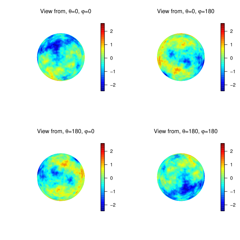
where has been chosen to ensure that Table 1 shows the computational time (in seconds) needed for each method to generate the GRF on each grid. Reported times are based on a server with 32 cores 2x Intel Xeon e5‑2630v3, 2.4 Ghz processor and 32 GB RAM. Algorithm 1 is always faster. For the largest mesh, the eigenvalue and the Cholesky decomposition methods do not work because of storage problems. An example of a realization of the GRF is showed in Figure 2.
| Parameters | Circ. Embed. | Cholesky | Eigen |
|---|---|---|---|
| N=18, M=6 | 0.016 | 0.008 | 0.032 |
| N=40, M=13 | 0.021 | 0.541 | 1.047 |
| N=60, M=20 | 0.057 | 2.397 | 5.832 |
| N=120, M=40 | 0.121 | 24.781 | 278.228 |
| N=360, M=180 | 16.433 | – | – |
To study the simulation accuracy, we make use of variograms as defined through (1). Specifically, we estimate the variogram nonparametrically through
| (37) |
where is the indicator function of the set , is a bandwidth parameter and
We perform our simulations, using (that is, ), corresponding to a degree regular longitude-latitude grid on the sphere, under three covariance models (Gneiting,, 2013):
- 1.
The exponential covariance function defined by (36)
- 2.
The generalized Cauchy model defined by
- 3.
The Matern model defined as
where is the Bessel function of second kind of order and is the Gamma function. In this simulation study we use , , , , and . Such setting ensures that for . Note that the regularity parameter is restricted to the interval to ensure positive definiteness on (Gneiting,, 2013).
For each simulation, Cholesky decomposition is used to compute and the variogram estimates in Equation (37) are computed. 100 simulations have been performed for each covariance model using Algorithm 1 and using direct Cholesky decomposition for comparison. Figure 3(a) – 3(c) show the estimated variogram for each simulation and the average variogram as well. Also, global rank envelopes (Myllymäki et al.,, 2017) where computed for the variogram under each simulation algorithms. The average variograms match almost perfectly. The superimposition of the envelopes shows that our approach generates the same variability as the Cholesky decomposition.
A similar simulation study is provided for a temporal stationary and spatially isotropic random field on We provide a non-parametric estimate of (23) through
where and
We simulate using the spherical grid and the temporal grid where , that is, . We use the following family of covariance functions (Porcu et al.,, 2016):
| (38) |
where , and is any temporal covariance function. In this case we consider and . We set , and . Such setting ensures that for . Following Porcu et al., (2016), Equation (38) is a positive semi-definite covariance function, and so we use SVD decomposition to compute . In addition to Table 1, the number of points used in this experiment does not allow to use Cholesky decomposition, and so envelopes were not computed this time. Figure 4 shows the estimated variogram for 100 simulations, concluding that we are simulating from the wanted distribution.
Finally, we use the method to simulate a spatio-temporal process with , , where , that is, , for and respectively. Such realizations are shown in Movie 1 and Movie 2 respectively.
6 Discussion
Circulant embedding technique was developed on and for an isotropic covariance function and for a spatially isotropic and temporally stationary covariance function respectively. All the calculations were done using the geodesic distance on the sphere. However, this method can be used with the chordal distance and axially symmetric covariance functions (Huang et al.,, 2012). As shown in our simulation study, this method allows to simulate seamlessly up to points in a spatio-temporal context. Traditional functional summary statistics, like the variogram, require a high computational cost which motivates the development of different functional summary statistics or algorithms than can deal with a huge number of points.
Extensions to non-regular grids could be done using the technique detailed in Dietrich and Newsam, (1996), which could be easily modified to and . In addition, for an integer , can be computed using circulant embedding by computing or . Such result is also useful to compute with Such case corresponds to the inverse of a matrix (Jun and Stein,, 2008) which is important for the computation of maximum likelihood estimators and Kriging predictors (Stein,, 2012).
7 Acknowledgments
First author was supported by The Danish Council for Independent Research — Natural Sciences, grant DFF – 7014-00074 ”Statistics for point processes in space and beyond”, and by the ”Centre for Stochastic Geometry and Advanced Bioimaging”, funded by grant 8721 from the Villum Foundation. Third author was supported by FONDECYT number 1170290.


References
- Chiles, (1999) Chiles, J.P. Delfiner, P. (1999). Geostatistics: Modelling Spatial Uncertainty. Wiley, New York.
- Clarke et al., (2018) Clarke, J., Alegría, A., and Porcu, E. (2018). Regularity properties and simulations of Gaussian random fields on the sphere cross time. Electronic Journal of Statististics, 12:399–426.
- Coxeter, (1973) Coxeter, H. S. M. (1973). Regular Polytopes. Methuen, London.
- Creasey and Lang, (2018) Creasey, P. E. and Lang, A. (2018). Fast generation of isotropic Gaussian random fields on the sphere. Monte Carlo Methods and Applications, 24(1):1–11.
- Davis, (1979) Davis, P. J. (1979). Circulant Matrices. Wiley, New York.
- Dietrich and Newsam, (1996) Dietrich, C. and Newsam, G. (1996). A fast and exact method for multidimensional Gaussian stochastic simulations: extension to realizations conditioned on direct and indirect measurements. Water resources research, 32(6):1643–1652.
- Dietrich and Newsam, (1997) Dietrich, C. and Newsam, G. N. (1997). Fast and exact simulation of stationary Gaussian processes through circulant embedding of the covariance matrix. SIAM Journal on Scientific Computing, 18:1088–1107.
- Emery et al., (2016) Emery, X., Arroyo, D., and Porcu, E. (2016). An improved spectral turning-bands algorithm for simulating stationary vector Gaussian random fields. Stochastic environmental research and risk assessment, 30(7):1863–1873.
- Gneiting, (2013) Gneiting, T. (2013). Strictly and non-strictly positive definite functions on spheres. Bernoulli, 19:1327–1349.
- Gneiting et al., (2006) Gneiting, T., Ševčíková, H., Percival, D. B., Schlather, M., and Jiang, Y. (2006). Fast and exact simulation of large Gaussian lattice systems in : exploring the limits. Journal of Computational and Graphical Statistics, 15(3):483–501.
- Huang et al., (2011) Huang, C., Zhang, H., and Robeson, S. M. (2011). On the validity of commonly used covariance and variogram functions on the sphere. Mathematical Geosciences, 43:721–733.
- Huang et al., (2012) Huang, C., Zhang, H., and Robeson, S. M. (2012). A simplified representation of the covariance structure of axially symmetric processes on the sphere. Statistics & Probability Letters, 82(7):1346–1351.
- Jun and Stein, (2008) Jun, M. and Stein, M. L. (2008). Nonstationary covariance models for global data. The Annals of Applied Statistics, 2:1271–1289.
- Lang and Schwab, (2015) Lang, A. and Schwab, C. (2015). Isotropic Gaussian random fields on the sphere: regularity, fast simulation and stochastic partial differential equations. The Annals of Applied Probability, 25:3047–3094.
- Møller et al., (2015) Møller, J., Nielsen, M., Porcu, E., and Rubak, E. (2015). Determinantal point process models on the sphere. Bernoulli, 24:1171–1201.
- Myllymäki et al., (2017) Myllymäki, M., Mrkvička, T., Grabarnik, P., Seijo, H., and Hahn, U. (2017). Global envelope tests for spatial processes. Journal of the Royal Statistical Society: Series B (Statistical Methodology), 79(2):381–404.
- Park and Tretyakov, (2015) Park, M. H. and Tretyakov, M. (2015). A block circulant embedding method for simulation of stationary Gaussian random fields on block-regular grids. International Journal for Uncertainty Quantification, 5:527–544.
- Porcu et al., (2016) Porcu, E., Bevilacqua, M., and Genton, M. G. (2016). Spatio-temporal covariance and cross-covariance functions of the great circle distance on a sphere. Journal of the American Statistical Association, 111(514):888–898.
- Stein, (2012) Stein, M. L. (2012). Interpolation of Spatial Data: Some Theory for Kriging. Springer Science & Business Media.
- Wood and Chan, (1994) Wood, A. T. and Chan, G. (1994). Simulation of stationary Gaussian processes in [0,1]d. Journal of Computational and Graphical Statistics, 3:409–432.
- Zhihao, (1990) Zhihao, C. (1990). A note on symmetric block circulant matrix. J. Math. Res. Exposition, 10:469–473.