Exploiting statistical dependencies of time series
with hierarchical correlation reconstruction
Abstract
While we are usually focused on forecasting future values of time series, it is often valuable to additionally predict their entire probability distributions, e.g. to evaluate risk, Monte Carlo simulations. On example of time series of 30000 Dow Jones Industrial Averages, there will be presented application of hierarchical correlation reconstruction for this purpose: MSE estimating polynomial as joint density for (current value, context), where context is for example a few previous values. Then substituting the currently observed context and normalizing density to 1, we get predicted probability distribution for the current value. In contrast to standard machine learning approaches like neural networks, optimal polynomial coefficients here have inexpensive direct formula, have controllable accuracy, are unique and independently calculated, each has a specific cumulant-like interpretation, and such approximation can asymptotically approach complete description of any real joint distribution - providing universal tool to quantitatively describe and exploit statistical dependencies in time series, systematically enhancing ARMA/ARCH-like approaches, also based on different distributions than Gaussian which turns out improper for daily log returns. There is also discussed application for non-stationary time series like calculating linear time trend, or adapting coefficients to local statistical behavior.
Keywords: time series analysis, machine learning, ARMA-ARCH, density estimation, risk evaluation, data compression, non-stationary time series, trend analysis, wallet analysis
I Introduction

Modeling spatial or temporal statistical dependencies between observed values is a difficult task required in many applications. Standard approaches like correlation matrix, PCA (principal component analysis) approximate this behavior with multivariate gaussian distribution. Further corrections can be extracted by approaches like GMM (gaussian mixture model), KDE (kernel density estimation) [1] or ICA (independent component analysis) [2], but they have many weaknesses like lack of error control, large freedom of parameters and varying their number, or focusing on a specific types of distributions.
Approximating observed data sample with a polynomial is universal approach used in many fields of science, can provide as close description as needed. It turns out also very advantageous for density estimation, including multivariate joint distribution ([3, 4]), especially if variables are normalized to approximately uniform distribution on with CDF of approximated distribution like in copula theory [5], to properly model tails, optimize weights and standardize coefficients.
Using orthonormal basis , it turns out that mean-square (MSE, ) optimization leads to estimated coefficients being just averages over the observed sample: . For multiple variables we can use basis of products of 1D orthornormal polynomials. On example of DJIA time series 11 1 Source of DJIA time series: http://www.idvbook.com/teaching-aid/data-sets/the-dow-jones-industrial-average-data-set/, with results summarized in Fig. 1, it will be used for prediction of current probability distribution based on a few previous values.
Financial time series are usually modelled with ARMA-ARCH-like simple models [6] for this purpose, exploiting pairwise dependencies between first two moments. Presented approach allows to systematically expand it in MSE-optimal way for including any moments among any number of variables, also for non-stationary time series. Additionally, standard models are usually based on Gaussian distribution, which turns out improper e.g. for daily log returns as we can see in a few figures here (especially Fig. 11) - presented approach can be based on any distribution (e.g. Laplace), using it for normalization of variables.
Finally, asymptotically (with basis and sample size ) we can approach complete description of any statistical dependencies - any real joint distribution of observed variables. Coefficients can be cheaply calculated as just averages, are unique and independently calculated, for stationary time series we can control their accuracy. Each has also a specific interpretation: resembling cumulants, but being much more convenient for reconstructing probability distribution - instead of the difficult problem of moments [7], here they are just coefficients of polynomial as density. Inconvenience of parameterizing density with polynomial are occurring negative predictions, which can be interpreted as small positive - we can optimize this calibration based on the data sample as discussed later (Fig. 4, 5).
In the discussed example: analysis of DJIA time series, we will first normalize the variables to nearly uniform probability distribution on : by considering differences of logarithms (so called log returns), and transforming them by CDF (cumulative distribution function) of approximated distribution (usually Laplace) as shown in Fig. 2 (and 10). In copula theory [5] such normalization is made with empirical distribution, then there is used usually single parameter distribution to describe dependencies. Here we normalize with parametric distribution instead, repairing inaccuracy by fitting polynomial, described by as large number of parameters as needed - it allows for flexibility, including modelling evolution of polynomial coefficients for non-stationary time series. Additionally, thanks to normalization, coordinates correspond to quantiles e.g. 1/2 to median, length to percentage of population - providing proper weights for optimized distance.
After normalization , looking at successive positions of , if uncorrelated they would come from distribution on . Its corrections as linear combination of orthonormal basis of polynomials can be inexpensively and independently calculated, providing unique and asymptotically complete description of statistical dependencies between these neighboring values. Treating of them as earlier context, substituting their values and normalizing to 1, we get predictions of (conditional) probability distribution for the current value as summarized in Fig. 1.

Handling of non-stationary time series is also proposed: by replacing global average with local averages over past values with exponentially decaying weights, or using interpolation with time as additional dimension.
Presented approach can be naturally extended to multivariate time series, e.g. stock prices of separate companies to model their statistical dependencies, what is presented in [9] on example of yield curve parameters, here there will be presented example of modelling various statistical dependencies of 29 of Dow Jones companies.
More relaxed treatment of values of such polynomials as cumulant-like features and contributions, also combining with discrete variables, can be found in [10] for credibility evaluation of income data.
II Normalization to nearly uniform density
We will first work on example of Dow Jones Industrial Averages time series for . As financial data usually evolve in multiplicative not additive manner, we will work with to make it additive.
Time series are usually normalized to allow assumption of stationary process: such that joint probability distribution does not change when position is shifted. The standard approach, especially for gaussian distribution, is to subtract mean value, then divide by the standard deviation.
However, above normalization does not exploit local dependencies between values, what we are interested in. Using experience from data compression (especially lossless image e.g. JPEG LS [11]), we can use a predictor for the next value based on its local context: for example a few previous values (2D neighbors for image compression), or some more complex features (e.g. using averages over time windows, or dimensionality reduction methods like PCA), then model probability distribution of difference from the predicted value (residue).
Considering simple linear predictors: as in ARMA-like models, we can use optimize parameters to minimize mean square error. For 2D image such optimization leads to approximate parameters . For Dow Jones sequence such optimization leads to nearly negligible weights for all but the previous value. Hence, for simplicity we will just operate on logarithmic returns:
| (1) |
time series, where the number of possible indexes has been reduced by 1 due to shift: .
Such sequences of differences from predictions (residues) are well known in data compression to have nearly Laplace distribution - density:
| (2) |
where maximum likelihood estimation of parameters is just: median of , mean of . We can see in Fig. 2 that CDF from sorted values has decent agreement with CDF of Laplace distribution. Otherwise, there can be used e.g. generalized normal distribution [12], also called exponential power distribution (EPD) or generalized error distributions, which includes both gaussian and Laplace distribution - its optimization is presented in Fig. 11. Student’s t or stable distributions (Levy) [13] might be also worth considering as they include heavy tail distributions. These distributions have also known asymmetric variants - which can be considered if two directions have essentially different tails.
We could also use a varying distribution for normalization , using for example CDF of Gaussian of width depending on previous value using coefficients from ARCH model. This way we could directly enhance some successful standard model - by using it for normalization, than fitting polynomial to exploit complex further statistical dependencies: missed by the low parameter model.
For simplicity there is mainly used Laplace distribution here to normalize our variables to nearly uniform in , what allows to compactify the tails, improve performance (weight proportional to population) and normalize further coefficients:
| (3) |
is CDF of used distribution (Laplace here). We can see in Fig. 2 (and later 10) that this final sequence has nearly uniform probability distribution. Its corrections will be included in further estimation of polynomial as (joint) probability distribution, like presented later in Fig. 6.
We will search for density. To remove transformation (3) to get final density, observe that . Differentiating over , we get
| (4) |
III Hierarchical correlation reconstruction
After normalization we have sequence with nearly uniform density, marked green in Fig. 2 here. Taking its succeeding values, if uncorrelated they would come from nearly uniform distribution on - difference from uniform distribution describes statistical dependencies in our time series. We will use polynomial to describe them: estimate joint density for succeeding values of .
Define for and , . They form vectors containing value with its context - we will model (joint) probability density of these vectors as polynomial. Generally we can also use more sophisticated contexts, for example average of a few earlier values (e.g. ) as a single context variable to include longer range correlations, or e.g. some macroeconomical variables to exploit also dependence from additional information. Dimensionality reduction techniques like PCA can be used to include dependence from a large number of variables. Normalization to nearly uniform density is recommended for the predicted values (), for context values it might be better to omit it, especially when absolute values are important like for image compression.
Finally assume we have vector sequence of value with its context, we would like to model density of such vectors as polynomial. It turns out [3] that using orthonormal basis, which for multidimensional case can be products of 1D orthonormal polynomials, mean square () optimization leads to extremely simple formula for estimated coefficients:
| (5) |
The basis used this way has functions, generally it seems worth to consider different for separate coordinates , or restrict to include correlations only from e.g. pairs by using j with at most two nonzero indexes. Beside inexpensive calculation, this simple approach has also very convenient property of coefficients being independently calculated, giving each j unique value and interpretation, and controllable error. Independence also allows for flexibility of considered basis - instead of using all j, we can focus on more promising ones: with larger absolute value of coefficient, replacing negligible . Instead of mean square optimization, we can use often preferred: likelihood maximization [4], but it requires additional iterative optimization and introduces dependencies between coefficients.
Above 1D polynomials are orthonormal in : , getting (rescaled Legendre): and for correspondingly:
Their plots are in the top of Fig. 3. corresponds to normalization. The coefficient decides about reducing or increasing the mean - has similar interpretation as expected value. Analogously coefficient decides about focusing or spreading given variable, similarly as variance. And so on: further has similar interpretation as -th cumulant, however, while reconstructing density from moments is a difficult problem, presented description is directly coefficients of polynomial estimating the density.
For multiple variables, describes only correlations between coordinates, does not affect coordinates, as we can see in the center of Fig. 3. Each such mixed coefficient has also a specific interpretations here, for example decides between increase and decrease of second variable with increase of the first, analogously decides focus or spread of the second variable.
Assuming stationary time series (fixed joint distribution of ), errors of such estimated coefficients come from approximately gaussian distribution:
| (6) |
For the integral has value 1, getting in our case. As we can see in bottom of Fig. 3, a few percents of coefficients here are more that tenfold larger: can be considered as essential, not a result of noise.
Here is a list of the largest coefficients for Dow Jones normalized series (beside ) in , case. It neglects shifted sequences, for example .

Positive:
Negative:


Each such unique coefficient describes a specific correction from uniform density: by . For example we can see large positive coefficients for all pairs of , what means upward directed parabola for both variables: quantitatively describes how large change in a given day increases probability of large changes in neighboring days. Further coefficients have more complex interpretations, for example large positive means that 6 large increases in a row are preferred, but 6 large decreases are less likely. In contrast, large negative means that larger change 5 days earlier reduces probability of 5 large increases in a row.

Having such density we can use it to predict probability distribution of the current symbol basing on the context (Fig. 1): by substituting context to the polynomial and normalizing the remaining 1D polynomial to integrate to 1. This predicted density as polynomial can sometimes go below zero, what needs a separate interpretation as low positive - we can obtain such proper calibration from the data sample, as discussed in Fig. 4, 5.
IV Adaptivity for non-stationary time series
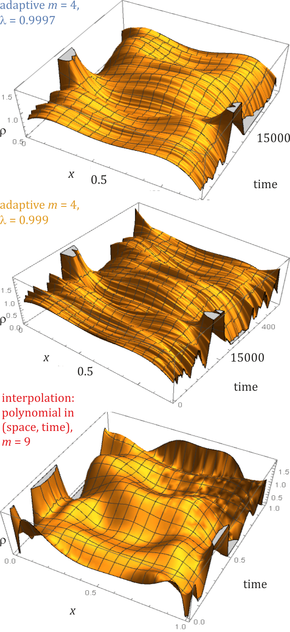

We have previously assumed stationary time series: that joint probability distribution within length moving time windows is fixed, what is often only approximation for real time series. As coefficients here are just averages over values: , for coefficients describing local behavior we can use (known in data compression) averaging with exponentially decaying weights [4]:
| (7) |
for some learning rate : close but smaller than 1 (e.g. ), starting for example with . Its proper choice is a difficult question: larger gives smoother behavior, but needs more time to adapt (delay).
For modeling of time trends or a posteriori analysis of historical data (with known future), we can alternatively estimate polynomial for multi-dimensional variable with time as one of coordinates, rescaled to range, e.g. . This way we estimate behavior of each coefficient as polynomial, allowing e.g. to interpolate to real time, or try to forecast that future trend (as low degree polynomial) will be similar as in the earlier period.
It might be tempting to use this approach also for extrapolation to predict future trends, e.g. rescale time to range instead, and look at behavior in time 1. However, such polynomial often has some uncontrollable behavior at the boundaries, suggesting caution while such extrapolation. Other orthonormal families (e.g. sines and cosines) have better boundary behavior - might be more appropriate for such extrapolation, however, discussed earlier modelling of joint distribution with context representing the past is generally a safer approach.
The following three figures present such analysis for discussed DJIA sequence. Figure 6 contains estimation of density as polynomial using stationarity assumption - models inaccuracy of Laplace used in normalization. Figure 7 contains its time evolution for non-stationary models: adaptive or interpolation. Figure 8 evaluates these approaches and shows time evolution for first 4 cumulant-like coefficients.
V Modelling multivariate dependencies

Example of predicting probability distribution for multivariate time series is presented in [9]. To continue the Dow Jones topic, there will be presented application of the discussed methodology to better understand complex statistical dependencies between stock prizes of 30 companies DJIA is calculated from, for example for more accurate wallet analysis. The selection of these companies has changed throughout the history - there will be used the one from September 2018. Daily prices for the last 10 years can be downloaded from NASDAQ webpage (www.nasdaq.com) for all but DowDuPont (DWDP) - there will be used daily close values for 2008-08-14 to 2018-08-14 period ( values) for the remaining 29 companies: 3M (MMM), American Express (AXP), Apple (AAPL), Boeing (BA), Caterpillar (CAT), Chevron (CVX), Cisco Systems (CSCO), Coca-Cola (KO), ExxonMobil (XOM), Goldman Sachs (GS), The Home Depot (HD), IBM (IBM), Intel (INTC), Johnson&Johnson (JNJ), JPMorgan Chase (JPM), McDonald’s (MCD), Merck&Company (MRK), Microsoft (MSFT), Nike (NKE), Pfizer (PFE), Procter&Gampble (PG), Travelers (TRV), UnitedHealth Group (UNH), United Technologies (UTX), Verizon (VZ), Visa (V), Walmart (WMT), Walgreens Boots Alliance (WBA) and Walt Disney (DIS). We will again work on logarithmic returns.


The standard approach to quantitatively describe statistical dependencies between variables is by correlation matrix - presented in Fig. 9. We can use discussed here cumulant-like coefficients for better undersetting of more complex statistical dependencies and their time trends, each of them having unique specific interpretation.
The simplest application is modelling pairwise statistical dependencies - this time spatial instead of temporal as before. After normalization of all variables to nearly uniform distribution (with Laplace CDF like previously), pairwise joint distribution would be nearly uniform on if they are uncorrelated. To this initial density we add independently calculated correction as products of two orthonormal polynomials - coefficients of the first three for all pairs are presented in Fig. 12 and 13. There are also presented linear time trends for two of them: using first coefficient with time rescaled to as additional variable like in the previous section. The diagonal terms have no meaning in this methodology - are filled with a constant value.
These additional coefficients allow for deeper understanding of statistical dependencies, like between growth of one variable and variance of the second (12) or between their variances (22) like in ARCH. Time trends (calculated for previous 10 years) may suggest direction of further evolution of these dependencies. These coefficients are similar to multivariate mixed cumulants, but having a direct translation to probability density.
Figure 9 also contains first 5 eigenvectors of covariance matrix as in standard PCA technique. They correspond to largest variance directions and often turn out to group dependent variables. Here we usually estimate density as higher degree polynomials (formally ), for which there are generalizations of eigenvector decomposition [14], but they are more difficult to calculate and interpret. Presented matrices use only subset of coefficients, allowing to use standard eigenvector decomposition, e.g. :
Presented matrices describe only pair-wise statistical dependencies, we can analogously model dependencies in triples e.g. or in larger groups, and their time evolutions.
Log-likelihood evaluation and examples of modelling pairwise joint distributions are presented in Fig. 11. We can see how problematic is being fixed on using only Gaussian distribution, what leaves a burden of far inferior predictions - in terms of both unconditional coverage (Fig. 10) and log-likelihood. If choosing base distribution accordingly to data (like Laplace), exploiting further statistical dependencies (3 diagrams) leaves not much place for further improvements (from to times larger average density) for this type of data. Generally possible improvement is bounded by conditional entropy: average over possible contexts of entropy of the new value, which asymptotically is minus average log-likelihood. For example if we would like to encode these values with accuracy, for large we would need on average minus log-likelihood bits per value.
The discussed here approach starts with normalizing all variables to nearly uniform distribution. Alternative approach is to multiply idealized distribution (e.g. multivariate Gaussian from PCA, or Laplace) by polynomial, estimating the coefficients [3].
VI Extensions
The used examples presented basic methodologies for educative reasons, which in real models can be optimized, for example:
- •
Selective choice of basis: we have used complete basis of polynomials, what makes its size impractically large especially for high dimensions. However, usually only a small percentage of coefficients is above noise - we can selectively choose and use a sparse basis of significant values instead - describing real statistical dependencies, mixed moments between only a small number of variables. Another option is to selectively reduce polynomial degree for some of variables, or for example restrict the real degree of the entire polynomial: instead of each coordinate.
- •
Long-range value prediction: combining with state-of-art prediction models exploiting long-range dependencies, for example using a more sophisticated (than just the previous value) predictor of the current value.
- •
Improving informational content of context used for prediction: instead of using a few previous values as the context, we can use some features e.g. describing long-range behavior like average over a time window, or for example obtained from dimensionality reduction methods like PCA (principal component analysis).
- •
Maybe directly combining with a successful e.g. ARMA/ARCH-like model: use it for normalization using its modeled distributions like ARCH Gaussian of varying width, then model e.g. with polynomial to extract and exploit further statistical dependencies from data sample.
- •
Multivariate time series usually allow for much better prediction, as presented in [9]. Adding for example macroeconomic variables should improve prediction.
This appendix contains Wolfram Mathematica source for basic discussed procedure and stationary process, optimized to use built-in vector operations:
im = Import["c:/djia-100.xls"];
v = Log[Transpose[im[[1]]][[2, 2 ;; -1]]];
Print[ListPlot[v]];
n0 = Length[v];
yt = Table[v[[i + 1]] - v[[i]], {i, n1 = n0 - 1}];
syt = Sort[yt];                (* for approximated CDF *)
mu = Median[yt];                 (* Laplace estimation *)
b = Mean[Abs[yt - mu]];
cdfL = If[y < mu, Exp[(y-mu)/b]/2, 1-Exp[-(y-mu)/b]/2];
Print["Laplace distribution: mu= ", mu, "  b= ", b];
Print[Show[
   ListPlot[Table[{syt[[i]], (i - 0.5)/n1}, {i, n1}]],
    Plot[cdfL, {y, -0.1,0.1},PlotStyle -> {Thin, Red}]]];
xt = Table[cdfL /. y -> yt[[i]],{i,n1}]; (* normalized *)
Print[ListPlot[Sort[xt]]]; Print[ListPlot[xt]];
cl = 3; d = 1 + cl;  (* dimension = 1 + context length *)
m = 4;                 (* maximal degree of polynomial *)
coefn = Power[m + 1, d]; Print[coefn, " coefficients"];
p = Table[Power[x, k], {k, 0, m}];
p = Simplify[Orthogonalize[p,Integrate[#1 #2,{x,0,1}]&]];
Print["used orthonormal polynomials: ", p];
n = n1 - cl;            (* final number of data points *)
(* table of contexts and their polynomials: *)
ct = Transpose[Table[xt[[i + cl ;; i ;; -1]], {i, n}]];
ctp = Table[
   If[j==1, Power[ct,0], p[[j]] /. x -> ct], {j, m+1}];
(* calculate coefficients: *)
coef = Table[jt = IntegerDigits[jn, m + 1, d] + 1;
       Mean[Product[ctp[[jt[[c]], c]], {c, d}]],
       {jn, 0, coefn - 1}];

(* find 1D polynomials for various times: *)
pt = Table[0, {i, m + 1}, {i, n}];
Do[jt = IntegerDigits[jn, m + 1, d] + 1;
  pt[[jt[[1]]]] +=
  coef[[jn+1]] * Product[ctp[[jt[[c]], c]],
  {c, 2, cl + 1}], {jn, 0, coefn - 1}];
(* probability normalization to 1: *)
Do[pt[[i]] /= pt[[1]], {i, m + 1, 1, -1}];
(* predicted densities for observed values: *)
rho = Sum[ctp[[i, 1]] * pt[[i]], {i, m + 1}];
Print[ListPlot[Sort[rho]]];
(* densities in 10 random times: *)
plst = RandomInteger[{1, n}, 10];
pl = Table[i = plst[[k]];
  Sum[pt[[j, i]]*p[[j]], {j, m + 1}], {k, Length[plst]}];
Plot[pl, {x, 0, 1}, PlotRange -> {{0, 1}, {0, 5}}]
References
- [1] M. Rosenblatt et al., “Remarks on some nonparametric estimates of a density function,” The Annals of Mathematical Statistics, vol. 27, no. 3, pp. 832–837, 1956.
- [2] A. Hyvärinen and E. Oja, “Independent component analysis: algorithms and applications,” Neural networks, vol. 13, no. 4, pp. 411–430, 2000.
- [3] J. Duda, “Rapid parametric density estimation,” arXiv preprint arXiv:1702.02144, 2017.
- [4] ——, “Hierarchical correlation reconstruction with missing data,” arXiv preprint arXiv:1804.06218, 2018.
- [5] F. Durante and C. Sempi, “Copula theory: an introduction,” in Copula theory and its applications. Springer, 2010, pp. 3–31.
- [6] T. C. Mills and T. C. Mills, Time series techniques for economists. Cambridge University Press, 1991.
- [7] J. Shohat, J. Tamarkin, and A. Society, The Problem of Moments, ser. Mathematical Surveys and Monographs. American Mathematical Society, 1943. [Online]. Available: https://books.google.pl/books?id=xGaeqjHm1okC
- [8] P. Christoffersen, Elements of financial risk management. Academic Press, 2011.
- [9] J. Duda and M. Snarska, “Modeling joint probability distribution of yield curve parameters,” arXiv preprint arXiv:1807.11743, 2018.
- [10] J. Duda and A. Szulc, “Credibility evaluation of income data with hierarchical correlation reconstruction,” arXiv preprint arXiv:1812.08040, 2018.
- [11] M. J. Weinberger, G. Seroussi, and G. Sapiro, “The loco-i lossless image compression algorithm: Principles and standardization into jpeg-ls,” IEEE Transactions on Image processing, vol. 9, no. 8, pp. 1309–1324, 2000.
- [12] M. K. Varanasi and B. Aazhang, “Parametric generalized gaussian density estimation,” The Journal of the Acoustical Society of America, vol. 86, no. 4, pp. 1404–1415, 1989.
- [13] B. Mandelbrot, “The pareto-levy law and the distribution of income,” International Economic Review, vol. 1, no. 2, pp. 79–106, 1960.
- [14] L. Qi, “Eigenvalues of a real supersymmetric tensor,” Journal of Symbolic Computation, vol. 40, no. 6, pp. 1302–1324, 2005.