ATF: acoustic transfer function
RTF: relative transfer function
BMVDR: binaural minimum variance distortionless response beamformer
PSD: power spectral density
GEVD: generalized eigenvalue decomposition
SC: spatial coherence
SNR: signal-to-noise ratio
CW: covariance whitening

RTF-Based Binaural MVDR Beamformer Exploiting an External Microphone in a Diffuse Noise Field

Nico Gößling Simon Doclo

Abstract

Besides suppressing all undesired sound sources, an important objective of a binaural noise reduction algorithm for hearing devices is the preservation of the binaural cues, aiming at preserving the spatial perception of the acoustic scene. A well-known binaural noise reduction algorithm is the binaural minimum variance distortionless response beamformer, which can be steered using the relative transfer function (RTF) vector of the desired source, relating the acoustic transfer functions between the desired source and all microphones to a reference microphone. In this paper, we propose a computationally efficient method to estimate the RTF vector in a diffuse noise field, requiring an additional microphone that is spatially separated from the head-mounted microphones. Assuming that the spatial coherence between the noise components in the head-mounted microphone signals and the additional microphone signal is zero, we show that an unbiased estimate of the RTF vector can be obtained. Based on real-world recordings, experimental results for several reverberation times show that the proposed RTF estimator outperforms the widely used RTF estimator based on covariance whitening and a simple biased RTF estimator in terms of noise reduction and binaural cue preservation performance.

University of Oldenburg, Department of Medical Physics and Acoustics and Cluster of Excellence Hearing4All, Oldenburg, Germany
Email: {nico.goessling, simon.doclo}@uni-oldenburg.de
Web: www.sigproc.uni-oldenburg.de

1 Introduction

^†^† This work was supported by the Collaborative Research Centre 1330 Hearing Acoustics. the Cluster of Excellence 1077 Hearing4all, funded by the German Research Foundation (DFG), and by the joint Lower Saxony-Israeli Project ATHENA.

Noise reduction algorithms for head-mounted assistive listening devices (e.g., hearing aids, cochlear implants, hearables) are crucial to improve speech intelligibility and speech quality in noisy environments. Binaural noise reduction algorithms are able to use the spatial information captured by all microphones on both sides of the head [1, 2]. Besides suppressing undesired sound sources, binaural noise reduction algorithms also aim at preserving the listener’s spatial perception of the acoustic scene to assure spatial awareness, to reduce confusions due to a possible mismatch between acoustical and visual information, and to enable the listener to exploit the binaural hearing advantage [3].
As shown in [4, 1, 2], the mvdr (mvdr) beamformer is able to preserve the binaural cues, i.e., the interaural level difference (ILD) and the interaural time difference (ITD), of the desired source. The mvdr beamformer can either be implemented using the atf between the desired source and all microphones or using the rtf, relating the atf to a reference microphone [5]. Since estimating the RTFs (unlike the ATFs) is feasible in practice, RTF estimation has become an important task in the field of multichannel speech enhancement [6, 7, 8, 9, 10, 11, 12, 13].
Aiming at improving the performance of (binaural) noise reduction algorithms, recently the use of an external microphone in combination with the head-mounted microphones has been explored [14, 15, 16, 17, 18, 19, 20, 21]. It has, e.g., been shown that using an external microphone is able to improve performance in terms of noise reduction [14, 16, 18, 19, 20, 21], source localisation [17] and binaural cue preservation [16, 18].
In this paper, we propose a computationally efficient method to estimate the RTF vector in a diffuse noise field using the external microphone. This method requires the external microphone to be located far enough from the head-mounted microphones, such that the spatial coherence between the noise components in the head-mounted microphone signals and the external microphone signal is low. Assuming this spatial coherence to be zero, we show how an unbiased RTF estimator can be derived. Using real-world recordings, we compare the proposed RTF estimator to a simple biased RTF estimator and to the widely used RTF estimator based on cw (cw) [8, 7, 9, 10, 11] for several reverberation times and snr. The results show that the proposed RTF estimator yields a larger SNR improvement and reduced binaural cue errors compared to the existing RTF estimators. When comparing the proposed RTF estimator to an oracle RTF estimator (using the clean speech signal as external microphone signal), only a small performance difference can be observed.

2 Configuration and Notation

Refer to caption — Figure 1: Top-view of the considered acoustic scenario and microphone configuration ( $M=2$ ).

We consider an acoustic scenario with one desired source $S(\omega)$ and diffuse background noise (e.g., cylindrically or spherically isotropic noise) in a reverberant enclosure. Moreover, we consider a binaural configuration, consisting of a left and a right device (each containing $M$ microphones), and an external microphone that is spatially separated from the head-mounted microphones, cf. Figure 1. The $m$ -th microphone signal of the left hearing device $Y_{{\rm{L}},m}(\omega)$ can be written in the frequency-domain as

Y_{{\rm{L}},m}(\omega)=X_{{\rm{L}},m}(\omega)+N_{{\rm{L}},m}(\omega)\,,\hskip 10.00002ptm\in\{1,\dots,M\},

(1)

where $X_{{\rm L},m}(\omega)$ denotes the desired speech component, $N_{{\rm L},m}(\omega)$ denotes the noise component and $\omega$ denotes the angular frequency. For conciseness we will omit $\omega$ in the remainder of the paper, wherever possible. The $m$ -th microphone signal of the right hearing device $Y_{{\rm{R}},m}$ and the external microphone $Y_{{\rm{E}}}$ are similarly defined by substituting $\rm R$ and $\rm E$ for $\rm L$ , respectively. The microphone signals of the hearing devices can be stacked in a vector, i.e.,

\mathbf{y}=\left[Y_{{\rm L},1},\;\dots,\;Y_{{\rm L},M},\;Y_{{\rm R},1},\;\dots,\;Y_{{\rm R},M}\right]^{T}\in\mathbb{C}^{2M}\,,

(2)

with $(\cdot)^{T}$ denoting the transpose of a vector. Using (1), the vector $\mathbf{y}$ can be written as

\mathbf{y}=\mathbf{x}+\mathbf{n}\,,

(3)

where the speech vector $\mathbf{x}$ and the noise vector $\mathbf{n}$ are defined similarly as in (2). Without loss of generality, we choose the first microphone on each hearing device as reference microphone, i.e.,

Y_{\rm L}=\mathbf{e}_{\rm L}^{T}\mathbf{y}\,,\hskip 10.00002ptY_{\rm R}=\mathbf{e}_{\rm R}^{T}\mathbf{y}\,,

(4)

where $\mathbf{e}_{\rm L}$ and $\mathbf{e}_{\rm R}$ are selection vectors consisting of zeros and one element equal to 1, i.e., $\mathbf{e}_{\rm L}(1)=1$ and $\mathbf{e}_{\rm R}(M+1)=1$ . In the case of a single desired source, the speech vector $\mathbf{x}$ is equal to

\mathbf{x}=\mathbf{a}S\,,

(5)

where the vector $\mathbf{a}\in\mathbb{C}^{2M}$ contains the atf between the desired source $S$ and all microphones, including reverberation, microphone characteristics and head-shadowing. The rtf vectors $\mathbf{a}_{\rm L}$ and $\mathbf{a}_{\rm R}$ of the desired source are defined by relating the atf vector $\mathbf{a}$ to both reference microphones, i.e.,

\mathbf{a}_{\rm L}=\frac{\mathbf{a}}{\mathbf{e}_{\rm L}^{T}\mathbf{a}}\,,\hskip 10.00002pt\mathbf{a}_{\rm R}=\frac{\mathbf{a}}{\mathbf{e}_{\rm R}^{T}\mathbf{a}}\,.

(6)

The speech covariance matrix $\mathbf{R}_{\rm x}\in\mathbb{C}^{2M\times 2M}$ and the noise covariance matrix $\mathbf{R}_{\rm n}\in\mathbb{C}^{2M\times 2M}$ are defined as

	$\displaystyle\mathbf{R}_{\rm x}$	$\displaystyle=\mathcal{E}\{\mathbf{x}\mathbf{x}^{H}\}=\phi_{\rm x,L}\mathbf{a}_{\rm L}\mathbf{a}_{\rm L}^{H}=\phi_{\rm x,R}\mathbf{a}_{\rm R}\mathbf{a}_{\rm R}^{H}\,,$		(7)
	$\displaystyle\mathbf{R}_{\rm n}$	$\displaystyle=\mathcal{E}\{\mathbf{n}\mathbf{n}^{H}\}\,,$		(8)

where $\mathcal{E}\{\cdot\}$ denotes the expectation operator, $(\cdot)^{H}$ denotes the conjugate transpose, and $\phi_{\rm x,L}=\mathcal{E}\{|X_{\rm L}|^{2}\}$ and $\phi_{\rm x,R}=\mathcal{E}\{|X_{\rm R}|^{2}\}$ denote the psd (psd) of the desired source in the reference microphones. Assuming statistical independence between the desired speech and noise components, the microphone signal covariance matrix is equal to

\mathbf{R}_{\rm y}=\mathcal{E}\{\mathbf{y}\mathbf{y}^{H}\}=\mathbf{R}_{\rm x}+\mathbf{R}_{\rm n}\,.

(9)

The output signals at the left and the right hearing device are obtained by filtering and summing all microphone signals using the complex-valued filter vectors $\mathbf{w}_{\rm L}$ and $\mathbf{w}_{\rm R}$ , respectively, i.e.,

Z_{\rm L}=\mathbf{w}_{\rm L}^{H}\mathbf{y}\,,\hskip 10.00002ptZ_{\rm R}=\mathbf{w}_{\rm R}^{H}\mathbf{y}\,.

(10)

3 Binaural MVDR Beamformer

In this section, we briefly review the well-known BMVDR beamformer [22, 2, 23]. The mvdr beamformer minimizes the output noise psd while preserving the desired speech component in the reference microphones, hence preserving the binaural cues of the desired source. The constrained optimization problem for the left filter vector is given by

\min_{\mathbf{w}_{\rm L}}\;\mathcal{E}\{|\mathbf{w}_{\rm L}^{H}\mathbf{n}|^{2}\}\hskip 10.00002pt\text{subject to}\hskip 10.00002pt\mathbf{w}_{\rm L}^{H}\mathbf{a}_{\rm L}=1\,.

(11)

The constrained optimization problem for the right filter vector is defined similarly by substituting $\rm R$ for $\rm L$ . The solutions of these optimization problems are equal to [1, 2, 5]

\displaystyle\mathbf{w}_{\rm L}=\frac{\mathbf{R}_{\rm n}^{-1}\mathbf{a}_{\rm L}}{\mathbf{a}_{\rm L}^{H}\mathbf{R}_{\rm n}^{-1}\mathbf{a}_{\rm L}}\,,\hskip 10.00002pt\mathbf{w}_{\rm R}=\frac{\mathbf{R}_{\rm n}^{-1}\mathbf{a}_{\rm R}}{\mathbf{a}_{\rm R}^{H}\mathbf{R}_{\rm n}^{-1}\mathbf{a}_{\rm R}}\,.

(12)

Hence, to calculate the BMVDR beamformer an estimate of the noise covariance matrix $\mathbf{R}_{\rm n}$ and the rtf vectors $\mathbf{a}_{\rm L}$ and $\mathbf{a}_{\rm R}$ of the desired source is required. Usually, the noise covariance matrix $\mathbf{R}_{\rm n}$ is either estimated by recursively updating the matrix during speech pauses or approximated by using an appropriate model, e.g., assuming a spherically isotropic noise field. Similarly, the RTF vectors $\mathbf{a}_{\rm L}$ and $\mathbf{a}_{\rm R}$ are either estimated from the microphone signals or approximated by using – simulated or measured – anechoic RTFs corresponding to the assumed position of the desired source (e.g., in front of the user). In the following sections we will consider data-dependent RTF estimation approaches to steer the mvdr beamformer in (12).

4 RTF Estimation Approaches

In this section, we discuss different approaches to estimate the rtf vectors $\mathbf{a}_{\rm L}$ and $\mathbf{a}_{\rm R}$ of the desired source. First, we consider a biased estimator, which only requires an estimate of the microphone signal covariance matrix $\mathbf{R}_{\rm y}$ . Second, we consider the CW estimator [8, 10], which requires estimates of the microphone signal covariance matrix $\mathbf{R}_{\rm y}$ and the noise covariance matrix $\mathbf{R}_{\rm n}$ . Third, we present an RTF estimator that exploits the external microphone signal $Y_{\rm E}$ , assuming the spatial coherence between the noise components in the head-mounted microphone signals and the external microphone signal is zero.

4.1 Biased Estimator (B)

Using (6) and (7), it can be easily shown that the RTF vectors are equal to

\mathbf{a}_{\rm L}=\frac{\mathbf{R}_{\rm x}\mathbf{e}_{\rm L}}{\mathbf{e}_{\rm L}^{T}\mathbf{R}_{\rm x}\mathbf{e}_{\rm L}}\,,\hskip 10.00002pt\mathbf{a}_{\rm R}=\frac{\mathbf{R}_{\rm x}\mathbf{e}_{\rm R}}{\mathbf{e}_{\rm R}^{T}\mathbf{R}_{\rm x}\mathbf{e}_{\rm R}}\,,

(13)

i.e., a column of the speech covariance matrix $\mathbf{R}_{\rm x}$ normalized with the element corresponding to the respective reference microphone. When no reliable estimate of the speech covariance matrix $\mathbf{R}_{\rm x}$ is available, a simple but biased RTF estimate can be obtained by using the (noisy) microphone signal covariance matrix $\mathbf{R}_{\rm y}$ [24]

\mathbf{a}_{\rm L}^{\rm B}=\frac{\mathbf{R}_{\rm y}\mathbf{e}_{\rm L}}{\mathbf{e}_{\rm L}^{T}\mathbf{R}_{\rm y}\mathbf{e}_{\rm L}}\,,\hskip 10.00002pt\mathbf{a}_{\rm R}^{\rm B}=\frac{\mathbf{R}_{\rm y}\mathbf{e}_{\rm R}}{\mathbf{e}_{\rm R}^{T}\mathbf{R}_{\rm y}\mathbf{e}_{\rm R}}\,.

(14)

The biased estimator in (14) obviously does not lead to the same solution as (13), especially for low input snr.

4.2 Covariance Whitening (CW)

A frequently used (unbiased) RTF estimator is based on covariance whitening [8, 7, 9, 10, 11]. Using a square-root decomposition (e.g., Cholesky decomposition), the noise covariance matrix $\mathbf{R}_{\rm n}$ can be written as

\mathbf{R}_{\rm n}=\mathbf{R}_{\rm n}^{H/2}\mathbf{R}_{\rm n}^{1/2}\,.

(15)

The pre-whitened microphone signal covariance matrix is then equal to

\mathbf{R}_{\rm y}^{\rm w}=\mathbf{R}_{\rm n}^{-H/2}\mathbf{R}_{\rm y}\mathbf{R}_{\rm n}^{-1/2}\,,

(16)

which can be decomposed using the eigenvalue decomposition (EVD) as

\mathbf{R}_{\rm y}^{\rm w}=\mathbf{V}\mathbf{\Lambda}\mathbf{V}^{H}\,,

(17)

where the matrix $\mathbf{V}\in\mathbb{C}^{2M\times 2M}$ contains the eigenvectors and the diagonal matrix $\mathbf{\Lambda}\in\mathbb{R}^{2M\times 2M}$ contains the corresponding eigenvalues. Using the principal eigenvector $\mathbf{v}_{\rm max}$ , i.e., the eigenvector corresponding to the largest eigenvalue, the RTF vectors can be estimated as [11]

\mathbf{a}_{\rm L}^{\rm CW}=\frac{\mathbf{R}_{\rm n}^{1/2}\mathbf{v}_{\rm max}}{\mathbf{e}_{\rm L}^{T}\mathbf{R}_{\rm n}^{1/2}\mathbf{v}_{\rm max}}\,,\hskip 10.00002pt\mathbf{a}_{\rm R}^{\rm CW}=\frac{\mathbf{R}_{\rm n}^{1/2}\mathbf{v}_{\rm max}}{\mathbf{e}_{\rm R}^{T}\mathbf{R}_{\rm n}^{1/2}\mathbf{v}_{\rm max}}\,.

(18)

Due to the EVD, this estimator has a larger computational complexity than the biased estimator. Additionally, an estimate of both the microphone signal covariance matrix $\mathbf{R}_{\rm y}$ and the noise covariance matrix $\mathbf{R}_{\rm n}$ is required, although this estimate is required anyway for the BMVDR beamformer, cf. (12).

4.3 Spatial Coherence (SC)

Considering a spherically isotropic noise field as an example for a diffuse noise field, the magnitude-squared coherence (MSC) between the noise components in two different microphones (neglecting head-shadowing) is equal to [25]

{\rm MSC}=\left|{\rm sinc}\left(\frac{\omega d}{c}\right)\right|^{2}\,,

(19)

where $d$ denotes the distance between the two microphones and $c$ denotes the speed of sound. Figure 2 depicts the MSC for $d\in\left\{0.01,\;0.1,\;1\right\}$\mathrm{m}$$ and $c=$343\text{\,}\mathrm{m}\text{\,}{\mathrm{s}}^{-1}$$ . It can be seen that for large distances between the microphones the MSC tends to be very small, especially for high frequencies.
For now, let us assume that the external microphone is sufficiently far away from the head-mounted microphones, such that

\mathcal{E}\{\mathbf{n}N_{\rm E}^{*}\}=\mathbf{0}\,,

(20)

i.e., the noise components in the head-mounted microphone signals are spatially uncorrelated with the noise component in the external microphone signal. Using (20) yields

\mathcal{E}\{\mathbf{y}Y_{\rm E}^{*}\}=\mathcal{E}\{\mathbf{x}X_{\rm E}^{*}\}+\mathcal{E}\{\mathbf{n}N_{\rm E}^{*}\}=\mathcal{E}\{\mathbf{x}X_{\rm E}^{*}\}\,.

(21)

Using (21) and $\mathbf{x}=X_{\rm L}\mathbf{a}_{\rm L}=X_{\rm R}\mathbf{a}_{\rm R}$ , the spatial-coherence-based RTF estimator (SC) is equal to

\boxed{\mathbf{a}_{\rm L}^{\rm SC}=\frac{\mathcal{E}\{\mathbf{y}Y_{\rm E}^{*}\}}{\mathcal{E}\{Y_{\rm L}Y_{\rm E}^{*}\}},\hskip 10.00002pt\mathbf{a}_{\rm R}^{\rm SC}=\frac{\mathcal{E}\{\mathbf{y}Y_{\rm E}^{*}\}}{\mathcal{E}\{Y_{\rm R}Y_{\rm E}^{*}\}}}

(22)

Of course, in practice the assumption made in (20) does not perfectly hold. Hence, in the experimental evaluation in Section 5 we also consider an oracle version of the estimator in (22), which uses the clean speech signal $S$ as the external microphone signal, such that (20) perfectly holds, i.e.,

\mathbf{a}_{\rm L}^{\rm SC_{opt}}=\frac{\mathcal{E}\{\mathbf{y}S^{*}\}}{\mathcal{E}\{Y_{\rm L}S^{*}\}}\,,\hskip 10.00002pt\mathbf{a}_{\rm R}^{\rm SC_{opt}}=\frac{\mathcal{E}\{\mathbf{y}S^{*}\}}{\mathcal{E}\{Y_{\rm R}S^{*}\}}\,.

(23)

Compared to the CW estimator, the SC estimator does not need an estimate of the noise covariance matrix $\mathbf{R}_{\rm n}$ and has a lower computational complexity, but obviously requires an external microphone to be available.

5 Experimental Results

In this section, an experimental evaluation is presented of the BMVDR beamformer in (12) using the RTF estimators discussed in Section 4. In Section 5.1 the recording setup is described, while detailed information about the implementation is provided in Section 5.2 and the results are presented in Section 5.3.

5.1 Recording setup

All signals were recorded in a laboratory located at the University of Oldenburg where the reverberation time can be easily changed by closing and opening absorber panels mounted to the walls and the ceiling. The room dimensions are about $(7\times 6\times 2.7)\;$\mathrm{m}$$ , where the reverberation time was set approximately to the three different values $T_{60}\in\{250,\;500,\;750\}$\mathrm{m}\mathrm{s}$$ . The reverberation times were measured using the broad band energy decay curve of measured impulse responses. At the center of the room a KEMAR head-and-torso simulator (HATS) was placed. Two behind-the-ear hearing aid dummies with two microphones each, i.e., $M=2$ , were placed on the ears of the HATS.
The desired source was a male English speaker played back by a loudspeaker placed at about $2\text{\,}\mathrm{m}$ from the center of the head at the same height and at an angle of $35\text{\,}\mathrm{\SIUnitSymbolDegree}$ , i.e., on to the right side of the HATS (cf. Figure 1). The external microphone was placed at about $0.5\text{\,}\mathrm{m}$ from the desired source, leading to a distance of about $1.5\text{\,}\mathrm{m}$ to the HATS, which refers to, e.g., a table microphone or a smartphone that is connected to the binaural hearing device. To generate the background noise, we used four loudspeakers facing the corners of the laboratory, playing back different multi-talker recordings. Figure 3 shows the long-term magnitude-squared coherence between the recorded noise in the reference microphone of the left hearing aid and the external microphone. It can be observed that the assumption in (20) obviously does not perfectly hold, but the coherence is fairly small. The desired source and the background noise were recorded separately in order to be able to mix them together at different input ${\rm SNRs}\in\{-5,0,5\}\;$\mathrm{d}\mathrm{B}$$ . The SNR in the external microphone signal was about $9.6\text{\,}\mathrm{d}\mathrm{B}$ higher than in the head-mounted microphone signals. Please note, that streaming and directly using the external microphone signal would not include any binaural cues. The complete signal had a length of $20\text{\,}\mathrm{s}$ with $0.5\text{\,}\mathrm{s}$ of noise-only at the beginning.

5.2 Implementation and Performance Measures

All signals were processed at a sampling rate of $16\text{\,}\mathrm{k}\mathrm{H}\mathrm{z}$ . We used the short-time Fourier transform (STFT) with frame length $T=256$ , corresponding to $16\text{\,}\mathrm{m}\mathrm{s}$ , overlapping by $R=128$ samples, e.g., for the left reference microphone signal

	$\displaystyle Y_{\rm L}(k,l)$	$\displaystyle=\sum_{t=0}^{T-1}y_{\rm L}(l\cdot R+t)w(t)e^{-j2\pi kt/T}\;,$		(24)
		$\displaystyle=X_{\rm L}(k,l)+N_{\rm L}(k,l)\,,$		(25)

with $k$ the frequency bin index, $l$ the time frame index, $y_{\rm L}(t)$ the left reference microphone signal in the time-domain, $w(t)$ a square-root Hann window of length $T$ and $j=\sqrt{-1}$ .
To distinguish between speech-plus-noise and noise-only frames we used an oracle broad band voice activity detection (VAD), based on the energy of the speech component in the right reference microphone signal. Using this VAD, the microphone signal covariance matrix $\hat{\mathbf{R}}_{\rm y}(k,l)$ and the noise covariance matrix $\hat{\mathbf{R}}_{\rm n}(k,l)$ were recursively estimated as

	$\displaystyle\hat{\mathbf{R}}_{\rm y}(k,l)$	$\displaystyle=\alpha_{\rm y}\hat{\mathbf{R}}_{\rm y}(k,l-1)+(1-\alpha_{\rm y})\mathbf{y}(k,l)\mathbf{y}^{H}(k,l)\,,$		(26)
	$\displaystyle\hat{\mathbf{R}}_{\rm n}(k,l)$	$\displaystyle=\alpha_{\rm n}\hat{\mathbf{R}}_{\rm n}(k,l-1)+(1-\alpha_{\rm n})\mathbf{y}(k,l)\mathbf{y}^{H}(k,l)\,,$		(27)

during detected speech-plus-noise frames and noise-only frames, respectively. The forgetting factors were chosen as $\alpha_{\rm y}=0.8521$ and $\alpha_{\rm n}=0.9841$ , corresponding to time constants of $50\text{\,}\mathrm{m}\mathrm{s}$ and $500\text{\,}\mathrm{m}\mathrm{s}$ , respectively. As initialization the corresponding long-term estimates of the covariance matrices were used.
The (time-varying) estimates of the covariance matrices were then used in the biased RTF estimator ( $\rm B$ ) in (14), the covariance-whitening-based RTF estimator ( $\rm CW$ ) in (18), the oracle spatial-coherence-based RTF estimator ( $\rm SC_{opt}$ ) in (23) and the spatial-coherence-based ( $\rm SC$ ) RTF estimator in (22). We then computed the (time-varying) BMVDR beamformer in (12) using the estimated RTF vectors and the estimated noise covariance matrix $\hat{\mathbf{R}}_{\rm n}(k,l)$ . The resulting BMVDR beamformer was then applied to the head-mounted microphone signals, i.e.,

Z_{\rm L}(k,l)=\mathbf{w}_{\rm L}^{H}(k,l)\mathbf{y}(k,l)\,,\hskip 10.00002ptZ_{\rm R}(k,l)=\mathbf{w}_{\rm R}^{H}(k,l)\mathbf{y}(k,l)\,.

(28)

The performance was evaluated in terms of noise reduction and binaural cue preservation. As a measure for noise reduction performance we used the intelligibility-weighted SNR improvement ( $\Delta{\rm iSNR}$ ) [26] between the right reference microphone signal and the output of the right hearing aid. As a measure for binaural cue preservation performance we used the reliable binaural cue errors of the direct sound of the desired speech component, i.e., $\rm\Delta ILD$ and $\rm\Delta ITD$ , based on an auditory model [27] and averaged over frequency.

5.3 Results

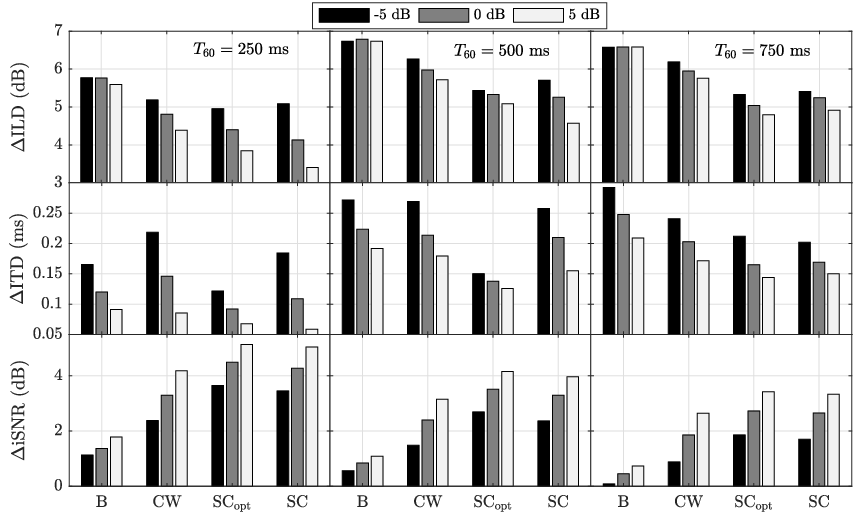
Figure 4 depicts the results for all four considered RTF estimators for different reverberation times and input SNRs. As expected, B generally shows worst performance in terms of binaural cue preservation and noise reduction performance.
Considering the ILD error, it can be observed for all estimators the ILD errors generally increase for increasing $T_{60}$ and decreasing input SNR. In addition it can be observed that the SC estimator consistently outperforms the CW estimator, especially for large $T_{60}$ . Moreover, almost no difference can be observed between the SC estimator and the oracle ${\rm SC_{opt}}$ estimator, for all $T_{60}$ and input SNRs.
Considering the ITD errors, it can be observed that for all estimators the ITD errors generally increase for increasing $T_{60}$ and decreasing input SNRs. Contrary to the ILD error, the SC estimator typically leads to larger ITD errors than the oracle ${\rm SC_{opt}}$ estimator, especially for $T_{60}=$250\text{\,}\mathrm{m}\mathrm{s}$$ and $500\text{\,}\mathrm{m}\mathrm{s}$ . Informal listening tests showed that when using SC (and ${\rm SC_{opt}}$ ) the desired source is perceived as a point source and sounded slightly less reverberated than the input of the reference microphones. For B and CW the binaural cue error sometimes showed large variations over frequency, which may lead to strange sounding artefacts, such that some frequencies are perceived as coming from another direction and the desired source sounds slightly diffuse.
Considering the iSNR improvement, it can be observed that for all estimators the SNR improvement generally decreases for increasing $T_{60}$ and decreasing input SNR. In addition, it can be observed that the SC estimator consistently outperforms the CW estimator for all $T_{60}$ and input SNRs. Moreover, almost no difference can be observed between the SC estimator and the oracle ${\rm SC_{opt}}$ estimator. From these results it can be concluded that the SC estimator outperforms the CW estimator. Moreover, for the considered scenario, i.e., the external microphone about $0.5\text{\,}\mathrm{m}$ from the desired source and about $1.5\text{\,}\mathrm{m}$ from the head-mounted microphones, the overall performance of the (practically implementable) SC estimator is very similar to the oracle ${\rm SC_{opt}}$ estimator, showing that the spatial coherence assumption in (20) is valid for the considered scenario. It can be expected that placing the external microphone closer to the desired source would slightly improve the performance of the SC estimator, especially in terms of binaural cue preservation.

6 Conclusions

In this paper we have shown how an external microphone signal can be exploited to estimate the RTF vectors of a desired source in a diffuse noise field. We assumed the spatial coherence between the noise components in the head-mounted microphone signals and the noise component in the external microphone signal to be zero to derive an unbiased RTF estimator. An experimental evaluation using real-world signals for several reverberation times and input SNRs showed that a better noise reduction performance and binaural cue preservation can be obtained when using the proposed RTF estimator compared to an RTF estimator based on covariance whitening and a simple biased RTF estimator.

References

[1] S. Doclo, W. Kellermann, S. Makino, and S. Nordholm, “Multichannel Signal Enhancement Algorithms for Assisted Listening Devices: Exploiting spatial diversity using multiple microphones,” IEEE Signal Processing Magazine, vol. 32, pp. 18–30, Mar. 2015.
[2] S. Doclo, S. Gannot, D. Marquardt, and E. Hadad, “Binaural Speech Processing with Application to Hearing Devices,” in Audio Source Separation and Speech Enhancement, ch. 18, Wiley, 2018.
[3] A. W. Bronkhorst and R. Plomp, “The effect of head-induced interaural time and level differences on speech intelligibility in noise,” The Journal of the Acoustical Society of America, vol. 83, no. 4, pp. 1508–1516, 1988.
[4] B. Cornelis, S. Doclo, T. Van den Bogaert, J. Wouters, and M. Moonen, “Theoretical analysis of binaural multi-microphone noise reduction techniques,” IEEE Transactions on Audio, Speech and Language Processing, vol. 18, pp. 342–355, Feb. 2010.
[5] S. Gannot, D. Burshtein, and E. Weinstein, “Signal Enhancement Using Beamforming and Non-Stationarity with Applications to Speech,” IEEE Transactions on Signal Processing, vol. 49, pp. 1614–1626, Aug. 2001.
[6] I. Cohen, “Relative transfer function identification using speech signals,” IEEE Transactions on Speech and Audio Processing, vol. 12, pp. 451–459, Sep. 2004.
[7] E. Warsitz and R. Haeb-Umbach, “Blind acoustic beamforming based on generalized eigenvalue decomposition,” IEEE Transactions on Audio Speech and Language Processing, vol. 15, pp. 1529–1539, July 2007.
[8] S. Markovich, S. Gannot, and I. Cohen, “Multichannel eigenspace beamforming in a reverberant noisy environment with multiple interfering speech signals,” IEEE Transactions on Audio, Speech, and Language Processing, vol. 17, pp. 1071–1086, Aug. 2009.
[9] A. Krueger, E. Warsitz, and R. Haeb-Umbach, “Speech enhancement with a GSC-like structure employing eigenvector-based transfer function ratios estimation,” IEEE Transactions on Audio Speech and Language Processing, vol. 19, pp. 206–219, Jan. 2011.
[10] R. Serizel, M. Moonen, B. Van Dijk, and J. Wouters, “Low-rank approximation based multichannel Wiener filter algorithms for noise reduction with application in cochlear implants,” IEEE/ACM Transactions on Audio, Speech and Language Processing, vol. 22, pp. 785–799, Apr. 2014.
[11] S. Markovich-Golan and S. Gannot, “Performance analysis of the covariance subtraction method for relative transfer function estimation and comparison to the covariance whitening method,” in Proc. IEEE International Conference on Acoustics, Speech and Signal Processing (ICASSP), (Brisbane, Australia), pp. 544–548, Apr. 2015.
[12] R. Giri, B. D. Rao, F. Mustiere, and T. Zhang, “Dynamic relative impulse response estimation using structured sparse Bayesian learning,” in Proc. IEEE International Conference on Acoustics, Speech and Signal Processing (ICASSP), (Shanghai, China), pp. 514–518, Mar. 2016.
[13] R. Varzandeh, M. Taseska, and E. A. P. Habets, “An iterative multichannel subspace-based covariance subtraction method for relative transfer function estimation,” in Proc. Joint Workshop on Hands-free Speech Communication and Microphone Arrays (HSCMA), (San Francisco, USA), pp. 11–15, Mar. 2017.
[14] A. Bertrand and M. Moonen, “Robust Distributed Noise Reduction in Hearing Aids with External Acoustic Sensor Nodes,” EURASIP Journal on Advances in Signal Processing, vol. 2009, p. 14 pages, Jan. 2009.
[15] N. Cvijanovic, O. Sadiq, and S. Srinivasan, “Speech enhancement using a remote wireless microphone,” IEEE Transactions on Consumer Electronics, vol. 59, pp. 167–174, Feb. 2013.
[16] J. Szurley, A. Bertrand, B. Van Dijk, and M. Moonen, “Binaural noise cue preservation in a binaural noise reduction system with a remote microphone signal,” IEEE/ACM Transactions on Audio, Speech and Language Processing, vol. 24, pp. 952–966, May 2016.
[17] M. Farmani, M. S. Pedersen, Z.-H. Tan, and J. Jensen, “Informed Sound Source Localization Using Relative Transfer Functions for Hearing Aid Applications,” IEEE/ACM Trans. on Audio, Speech, and Language Processing, vol. 25, pp. 611–623, Mar. 2017.
[18] N. Gößling, D. Marquardt, and S. Doclo, “Performance analysis of the extended binaural MVDR beamformer with partial noise estimation in a homogeneous noise field,” in Proc. Joint Workshop on Hands-free Speech Communication and Microphone Arrays (HSCMA), (San Francisco, USA), pp. 1–5, Mar. 2017.
[19] N. Gößling, D. Marquardt, and S. Doclo, “Comparison of RTF estimation methods between a head-mounted binaural hearing device and an external microphone,” in Proc. International Workshop on Challenges in Hearing Assistive Technology (CHAT), (Stockholm, Sweden), pp. 101–106, Aug. 2017.
[20] D. Yee, H. Kamkar-Parsi, R. Martin, and H. Puder, “A Noise Reduction Post-Filter for Binaurally-linked Single-Microphone Hearing Aids Utilizing a Nearby External Microphone,” IEEE/ACM Transactions on Audio Speech and Language Processing, vol. 26, no. 1, pp. 5–18, 2017.
[21] R. Ali, T. Van Watershoot, and M. Moonen, “Generalised sidelobe canceller for noise reduction in hearing devices using an external microphone,” in Proc. IEEE International Conference on Acoustics, Speech and Signal Processing (ICASSP), (Calgary, Canada), pp. 521–525, Apr. 2018.
[22] S. Doclo, S. Gannot, M. Moonen, and A. Spriet, “Acoustic beamforming for hearing aid applications,” in Handbook on Array Processing and Sensor Networks, pp. 269–302, Wiley, 2010.
[23] T. Klasen, T. van den Bogaert, M. Moonen, and J. Wouters, “Binaural noise reduction algorithms for hearing aids that preserve interaural time delay cues,” IEEE Transactions on Signal Processing, vol. 55, pp. 1579–1585, Apr. 2007.
[24] S. Braun, W. Zhou, and E. A. P. Habets, “Narrowband direction-of-arrival estimation for binaural hearing aids using relative transfer functions,” in Proc. IEEE Workshop on Applications of Signal Processing to Audio and Acoustics (WASPAA), pp. 1–5, Oct. 2015.
[25] B. F. Cron and C. H. Sherman, “Spatial-Correlation Functions for Various Noise Models,” Journal of the Acoustical Society of America, vol. 34, pp. 1732–1736, Nov. 1962.
[26] J. E. Greenberg, P. M. Peterson, and P. M. Zurek, “Intelligibility-weighted measures of speech-to-interference ratio and speech system performance,” Journal of the Acoustical Society of America, vol. 94, pp. 3009–3010, Nov. 1993.
[27] M. Dietz, S. D. Ewert, and V. Hohmann, “Auditory model based direction estimation of concurrent speakers from binaural signals,” Speech Communication, vol. 53, pp. 592–605, 2011.