Asymptotic electron motion in strong radiation-dominated regime

A. S. Samsonov Affiliation: Institute of Applied Physics of the Russian Academy of Sciences, 46 Ulyanov St., Nizhny Novgorod 603950, Russia E. N. Nerush Email: nerush@appl.sci-nnov.ru Affiliation: Institute of Applied Physics of the Russian Academy of Sciences, 46 Ulyanov St., Nizhny Novgorod 603950, Russia I. Yu. Kostyukov Affiliation: Institute of Applied Physics of the Russian Academy of Sciences, 46 Ulyanov St., Nizhny Novgorod 603950, Russia

August 24, 2026

Abstract

We study electron motion in electromagnetic (EM) fields in the radiation-dominated regime. It is shown that the electron trajectories become close to some asymptotic trajectories in the strong field limit. The description of the electron dynamics by this asymptotic trajectories significantly differs from the ponderomotive description that is barely applicable in the radiation-dominated regime. The particle velocity on the asymptotic trajectory is completely determined by the local and instant EM field. The general properties of the asymptotic trajectories are discussed. In most of standing EM waves (including identical tightly-focused counter-propagating beams) the asymptotic trajectories are periodic with the period of the wave field. Furthermore, for a certain model of the laser beam we show that the asymptotic trajectories are periodic in the reference frame moving along the beam with its group velocity that may explain the effect of the radiation-reaction trapping.

I Introduction

If the amplitude of an optical field is such that an electron gains in it energy of hundreds of its rest-mass energy, the electron starts to emit synchrotron radiation and can lose its energy efficiently [1]. This phenomenon — radiation reaction — is highly important for theoretical physics and astrophysics, therefore the motion of electrons in strong laser field nowadays is a topic of numerous theoretical investigations [2, 3, 4, 5, 6, 7], and it has been studied recently in the experiments [8, 9]. Also, the emission of hard photons by electrons in a strong laser field lets one to make a femtosecond broadband source of MeV photons, based on either laser pulse – electron beam collision [10, 11, 12], laser-plasma interaction [13, 14, 15, 16, 17] or electromagnetic cascades [18, 19].

In the interaction of a strong laser pulse with a plasma, radiation losses can significantly affect the plasma dynamics, and, for instance, lead to less-efficient ion acceleration [20, 21, 22, 23, 24], the enhancement of the laser-driven plasma wakefield [25, 26], highly efficient laser pulse absorption [27], relativistic transparency reduction [28], and to the inverse Faraday effect [29].

Despite of high importance of the radiation losses for laser-plasma physics at high intensity, there is no general concept of the losses impact on the electron motion, and this impact is considered mostly by ad hoc hypotheses and particle-in-cell (PIC) simulations. Only for a few field configurations the analytical solutions for motion of emitting electron are present [30, 31, 32], whereas for the motion of the non-emitting electron the Miller’s ponderomotive concept [33] is applicable in a vast number of cases.

In the high-intensity field, the energy gained by the electron can be significantly limited by the radiation losses. In this case, in contrast to the low-intensity limit, the electron Lorentz factor becomes small in comparison with the field amplitude: $\gamma/a_{0}\ll 1$ ; here $\gamma$ is the electron Lorentz factor and $a_{0}=eE_{0}/mc\omega$ is the normalized amplitude of the electric field, $E_{0}$ , $\omega$ is the typical angular frequency of the field, $c$ is the speed of light, $m$ and $e>0$ are the electron mass and the magnitude of the electron charge, respectively. The smallness of $\gamma/a_{0}$ allows one to simplify the analytical treatment of the electron motion in the strong radiation-dominated regime. This can be illustrated by a stationary Zel’dowich’s solution [30] for the electron motion in the rotating electric field $\mathbf{E}(t)$ . At moderate field intensity the angle $\varphi$ (between the particle velocity and the vector $-\mathbf{E}$ ) is connected with the electron Lorentz factor $\gamma$ . However, in the strong radiation dominated regime $\varphi$ and $\gamma/a_{0}$ tend to zero (see Fig. 1), and the particle velocity coincides with the direction of the electric field ( $\mathbf{v\parallel E}$ ), thus $\gamma$ is not needed in order to compute the particle trajectory.

In Refs. [34, 35] the concept of the electron motion, that in the radiation-dominated regime can supersede the ponderomotive concept, is discussed. It have been shown in Ref. [34] that in the regime of dominated radiation friction the number of degrees of freedom, which govern the electron motion, is reduced. Namely, it is shown for the rotating electric field with the Gaussian envelope, that on the time scales larger than the rotation period, the electron position is described by a first-order differential equation that does not contain the electron momentum. For this, the electron motion with Landau–Lifshitz radiation reaction have been considered. It is also shown that in the radiation-dominated regime, electrons are not expelled from but are captured for a long time by the strong-field region.

Refer to caption — Figure 1: Electrons moving in the rotating electric field and experiencing quantum radiation reaction for many periods of the rotation: (circles) the ratio of the mean Lorentz factor $\gamma_{m}$ to $a_{0}$ and (triangles) the mean angle $\varphi_{m}$ between the particle velocity and the vector opposite to the electric field, for different values of the field amplitude $a_{0}$ . Bars depict the standard deviations $\pm\sigma$ . Results of PIC-MC simulations for the field angular frequency $\omega=2\pi c/\lambda$ , $\lambda=1\text{ }\mu\text{m}$ .

In Ref. [35] it is shown for almost arbitrary field configuration, that in the strong field limit in a timescale, much smaller than the timescale of the field variation, the direction of the electron velocity approaches some certain direction that is determined only by the values of the local electric and magnetic fields. Then, as the electron velocity is known, the electron trajectory can be reconstructed. This approach, called the ‘‘low-energy limit’’, was used (but not described) for the fields of the linearly polarized standing waves earlier [36].

Let us emphasize that if the electron velocity is determined not by the electron momentum but by the local fields, one can describe the plasma dynamics with hydrodynamical equations. Indeed, in this case the currents in the Maxwell’s equations depend only on the particle density and particle velocity (i.e. on the particle density and local EM fields), therefore the first-order equation for the electron position together with the Maxwell’s equations and the continuity equation form a closed system of equations.

In this paper we present the first step toward such a hydrodynamical approach to the plasma dynamics in the radiation-dominated regime. Namely, in Sec. II we estimate $\gamma/a_{0}$ ratio and the threshold of the radiation-dominated regime. In Sec. III for arbitrary field configuration we find the first-order equation for the electron position, by a method different from Ref. [35] and with B-case (see below) considered separately. The right-hand-side of this equation is the velocity field that is fully determined by the local field vectors. It is shown that $\gamma\ll a_{0}$ is enough for this first-order equation to be valid in the laser field. In Sec. IV we compare the solution of this first-order equation with the solution of the exact equations of the electron motion for a number of field configurations. In Sec. V we discuss the relation between the velocity field and the Poynting vector. In Sec. VI the symmetry of the velocity field induced by the symmetry of the Maxwell’s equations, is considered, and the dramatic difference between the ponderomotive description and the description by the velocity field in the radiation-dominated regime is demonstrated. Thus, in the subsection VI.1, in the limit of strong fields, the electron motion in a wide class of periodic standing waves is shown to be periodic. From this, in the subsection VI.2 we show with a certain model of the laser beam that the beam can capture the electrons and carries them along itself with the beam group velocity. Sec. VII is the conclusion.

II Strong radiation-dominated regime

In order to estimate the threshold value of the normalized field amplitude $a_{0}$ for the radiation-dominated regime, let us start from the equations of the electron motion with the Landau–Lifshitz radiation reaction force incorporated:

	$\displaystyle\frac{d\mathbf{p}}{dt}=-\mathbf{E}-\mathbf{v}\times\mathbf{B}-F_{rr}\mathbf{v},$		(1)
	$\displaystyle\frac{d\gamma}{dt}=-\mathbf{v}\mathbf{E}-F_{rr}v^{2},$		(2)

where time is normalized to $1/\omega$ , $\mathbf{v}$ is the electron velocity normalized to the speed of light $c$ , $\mathbf{p}=\gamma\mathbf{v}$ is the electron momentum normalized to $mc$ , $\mathbf{E}$ and $\mathbf{B}$ are the electric and the magnetic fields respectively (normalized to $mc\omega/e$ ), and $F_{rr}\mathbf{v}$ is the main term of the radiation reaction force [37]:

F_{rr}=\alpha\gamma^{2}\frac{2}{3}\frac{\hbar\omega}{mc^{2}}\left\{(\mathbf{E+v\times B})^{2}-(\mathbf{Ev})^{2}\right\}.

(3)

Here $\alpha=e^{2}/\hbar c\approx 1/137$ is the fine-structure constant and $\omega$ is the frequency characterizing the time-scale or the space-scale of the field (e.g. angular frequency of the laser field).

The radiation losses increase sharply with the increase of $\gamma$ , therefore for some electron Lorentz factor $\gamma=\bar{\gamma}$ , the further energy gain stops due to the losses. The corresponding value $\bar{\gamma}$ can be found from Eq. (2) assuming that the transverse and the longitudinal to $\mathbf{v}$ components of the Lorentz force are of the order of $a_{0}$ :

\bar{\gamma}\approx\sqrt{\frac{3}{2\alpha a_{0}}\frac{mc^{2}}{\hbar\omega}},

(4)

where $a_{0}$ is the characteristic electric field strength. In the absence of the radiation reaction the electron energy in the field can be estimated as $\gamma\sim a_{0}$ , thus the radiation-dominated regime corresponds to $\bar{\gamma}\ll a_{0}$ hence

a_{0}\gg a_{0}^{*}=\left(\frac{3}{2\alpha}\frac{mc^{2}}{\hbar\omega}\right)^{1/3}.

(5)

Note for the laser wavelength $\lambda=1\text{ }\mu\text{m}$ the amplitude $a_{0}^{*}\approx 440$ that corresponds to the intensity $I\approx 5\times 10^{23}\text{ W}\,\text{cm}^{-2}$ . This level of intensity is expected to be reached in the near future with such facilities as ELI-beamlines [38], ELI-NP [39], Apollon [40], Vulcan 2020 [41], or XCELS [42].

In the case of strong radiation losses the angle between the Lorentz force and the electron velocity can be small, and the transverse to $\mathbf{v}$ component of the Lorentz force becomes much lower than the longitudinal one. However, this doesn’t affect much the given estimates. For instance, for the electron motion in the rotating electric field from the stationary Zel’dowich’s solution [30] we get $\varphi\approx\gamma/a_{0}$ and $\gamma\approx(a_{0}/\mu)^{1/4}\ll a_{0}$ (where $\mu=2\alpha\hbar\omega/3mc^{2}$ ) at $a_{0}\gg a_{0}^{*}$ , with the same estimate for $a_{0}^{*}$ (except the factor $3/2$ in the parentheses, see Ref. [30]). Note also that the quantum consideration of the radiation reaction gives results that are close to the Zel’dovich’s solution: in the Monte Carlo (MC) simulations the mean $\varphi$ value is about $\pi/2$ times larger than $\gamma/a_{0}$ , and $\gamma/a_{0}$ drops with the increase of the field amplitude (Fig. 1).

In what follows we assume that the field is far beyond the threshold of the radiation-dominated regime, $a_{0}\gg a_{0}^{*}$ .

III Velocity field and asymptotic trajectories

The reduced equations of the electron motion for arbitrary field configuration can be derived as follows. The equation for the electron velocity can be obtained from Eqs. (2) and (1), and is the following:

\frac{d\mathbf{v}}{dt}=-\frac{1}{\gamma}\left\{\mathbf{E-v(vE)+v\times B}+\frac{F_{rr}\mathbf{v}}{\gamma^{2}}\right\},

(6)

where the first three terms in the parentheses approximately correspond to the transverse to $\mathbf{v}$ component of the Lorentz force.

If the angle $\psi$ between the Lorentz force and the electron velocity is noticeable ( $\psi\sim 1$ ), then the term with $F_{rr}$ in Eq. (6) is negligible, because $F_{rr}/\gamma^{2}\sim a_{0}^{2}\alpha\hbar\omega/mc^{2}\ll a_{0}$ for reasonable field amplitudes, $E_{0}\lesssim E_{S}/\alpha$ , where $E_{S}=m^{2}c^{3}/e\hbar$ is the Sauter–Schwinger critical field. Thus, as far as $\gamma\ll a_{0}$ , we have $|d\mathbf{v}/dt|\gg 1$ .

It means that the characteristic timescale of the velocity vector variation is small, $\tau_{\mathbf{v}}\sim\gamma/a_{0}\ll 1$ . Therefore, on small time scales it can be assumed that the fields $\mathbf{E}$ and $\mathbf{B}$ in Eq. (6) are constant. In the constant EM field the electron velocity $\mathbf{v}$ in a time of some $\tau_{\mathbf{v}}$ approaches some asymptotic direction. This direction corresponds to $\psi\to 0$ hence $d\mathbf{v}/dt=0$ , and can be found as follows.

III.1 B-case

In the case $\mathbf{E\cdot B}=0$ and $B>E$ there is a reference frame $K^{\prime}$ in which the field is purely magnetic, and $\mathbf{B}^{\prime}\parallel\mathbf{B}$ (here strokes denote quantities in $K^{\prime}$ ). In $K^{\prime}$ the electron goes along the helical path with its axis parallel to the direction of $\mathbf{B}^{\prime}$ . The corresponding drift velocity of the electron in the laboratory reference frame $K$ is the speed of $K^{\prime}$ in $K$ and can be found from the following equation:

\mathbf{E+v\times B}=0.

(7)

Let us note that Eq. (7) does not depend on the component of the velocity parallel to the magnetic field, so one can choose this component arbitrarily (implying $v<1$ ). One can choose, for example, the solution with $\mathbf{v\cdot B}=0$ , i.e.:

\mathbf{v}=\frac{\mathbf{E\times B}}{B^{2}}.

(8)

As shown in Sec. VI.2 the ambiguity of $\mathbf{v}$ in this case can be resolved by additional physical considerations.

III.2 E-case

If $E\cdot B\neq 0$ or $E>B$ there is a reference frame $K^{\prime}$ , in which $\mathbf{E^{\prime}}\parallel\mathbf{B^{\prime}}$ or $B^{\prime}=0$ . The electron trajectory in $K^{\prime}$ asymptotically approaches the straight line parallel to $\mathbf{E}^{\prime}$ , and $v$ approaches $1$ . Note that for the resulting electron trajectory $\mathbf{v\cdot E}<0$ as far as the electron is accelerating by the field.

As $v\approx 1$ and the electron moves along the straight line, in the laboratory reference frame $K$ the resulting $\mathbf{v}$ can be found from the equation $d\mathbf{v}/dt=0$ , that yields

\mathbf{E-v(vE)+v\times B}=0,

(9)

Scalar multiplication of Eq. (9) by $\mathbf{B}$ , $\mathbf{E}$ and $\mathbf{E\times B}$ leads to the following solution:

	$\displaystyle\mathbf{vB=\frac{EB}{vE}},$		(10)
	$\displaystyle\mathbf{v\cdot E\times B}=E^{2}-(\mathbf{vE})^{2},$		(11)
	$\displaystyle\mathbf{vE}=-\sqrt{\frac{E^{2}-B^{2}+\sqrt{(E^{2}-B^{2})^{2}+4\mathbf{(EB)^{2}}}}{2}},$		(12)
	$\displaystyle\mathbf{v\cdot E\times[E\times B]}=\mathbf{(vE)(EB)-(vB)}E^{2}.$		(13)

The right-hand-side of Eq. (12) is relativistic invariant, and we choose the sign ‘‘ $-$ ’’ in order to obtain the stable trajectory in $K^{\prime}$ . For the opposite sign, ‘‘ $+$ ’’, the electron in $K^{\prime}$ is decelerating and its velocity is reversed quickly if initially $\mathbf{v}$ is not exactly parallel to the direction given by Eq. (9). Note that vectors $\mathbf{E}$ , $\mathbf{E\times B}$ , $\mathbf{E\times[E\times B]}$ form an orthogonal basis thus Eqs. (11)–(13) are enough to determine $\mathbf{v}$ unambiguously.

III.3 Asymptotic trajectory

Considering the electron motion on a timescale of the field variation timescale, $t\sim 1\gg\tau_{\mathbf{v}}$ , one can neglect the dynamics of the electron while it is approaching the constant-field-approximation asymptotic solution, and assume that in every time instant the electron velocity is determined by Eq. (7) or Eq. (9) which depend only on the instant (and local) fields. Thus, the electron trajectory is governed by the following reduced-order equations:

	$\displaystyle\frac{d\mathbf{r}}{dt}=\mathbf{v},$		(14)
	$\displaystyle\mathbf{E-v(vE)+v\times B}=0,$		(15)

where the last equation determines the velocity field $\mathbf{v}$ and can be used in both B- and E-cases (in B-case it yields Eq. (7)). From here on we call the solution of Eqs. (14)–(15) ‘‘asymptotic trajectory’’ because, first, locally it corresponds to the asymptotic ( $t\to\infty$ ) electron trajectory in the constant-field-approximation, and, second, it describes the electron trajectory in asymptotically strong field ( $a_{0}\gg a_{0}^{*}$ ).

Note that the reasoning about the electron trajectory in the radiation-dominated regime is also valid if the parameter $\chi$ is large ( $\chi\approx\gamma F_{\perp}/eE_{s}$ , see Ref. [43, 44], where $F_{\perp}$ is the component of the Lorentz force perpendicular to the particle velocity). In this case ( $\chi\gg 1$ ) the synchrotron emission is described by the quantum formulae and Eq. (3) is not valid, however, it is still possible to describe the electron trajectory classically between the photon emission events [45, 43] because $\ell_{f}\ll\ell_{W}$ . Here $\ell_{f}\sim mc^{2}/F_{\perp}$ is the radiation formation length, i.e. the distance within which the emission of a single photon occurs, and $\ell_{W}\sim c/W$ is the mean distance that the electron passes without the photon emission; $W$ is the full probability rate of the photon emission. Estimating

W\sim\frac{mce^{2}}{\hbar^{2}}\frac{\chi^{2/3}}{\gamma},

(16)

we obtain $\ell_{f}/\ell_{W}\sim\alpha/\chi^{1/3}<1/137\ll 1$ . Therefore, the electron moves classically between the short events of the photon emission. Note also that for optical frequencies $\ell_{W}/\lambda\sim\hbar\omega/(\alpha\chi^{2/3}mc^{2})\ll 1$ .

IV Simple examples

In order to test the asymptotic description of the electron trajectory (Eqs. (14) and (15)) we compare numerical solutions of them with numerical solutions of the classical equations of the electron motion with the radiation reaction taken into account by the inclusion of the Landau–Lifshitz force [37] or by the recoil of the emitted photons described in the quasiclassical framework of Baier–Katkov [43, 45]. Numerical solution of the full equations of the electron motion is based on the Vay’s pusher [46] where the Landau–Lifshitz force is taken into account with the Euler’s method or, alternatively, the quantum recoil is taken into account by the Monte Carlo (MC) technique similarly to the QUILL [47, 48] code (see also Appendix A). In order to solve Eqs. (14)–(15) we use the classical Runge–Kutta method. The test results for various field configurations are present below.

IV.1 Rotating electric field

In the rotating electric field of the amplitude $a_{0}$ Eq. (15) gives $\mathbf{v=-E}/E$ , that coincides with the high-field limit ( $a_{0}\gg a_{0}^{*}$ ) of the Zel’dovich’s stationary solution [30] utilizing the main term of the Landau–Lifshitz force. This stationary solution can be updated by taking into account quantum corrections to the radiation-reaction force [49], that also yields $\mathbf{v\to\mathbf{-}E}/E$ in the high-field limit. MC simulations demonstrate the same behavior, however, high dispersion of the angle between $\mathbf{v}$ and $\mathbf{E}$ is evident, see Fig. 1.

IV.2 Static B-node

Let us start from the following simple field configuration:

E_{y}=a_{0},\quad B_{z}=a_{0}x,

(17)

and the other components of the fields are zero.

In Fig. 2 the velocity field Eq. (8) ( $|x|>1$ ) and Eqs. (11) and (12) ( $|x|\leq 1$ ) is depicted by the arrows. In the left half of Fig. 2 the electron trajectories computed with the Landau–Lifshitz force are shown, and in the right half of Fig. 2 the electron trajectories are computed with Monte Carlo technique and quantum synchrotron formulae. Obviously, the shape of the electron trajectories computed with Monte Carlo approach is slightly different for different runs, so the bars depict the standard deviation of the electron final position. The trajectories are computed for different $a_{0}$ values, namely $a_{0}=500$ , $2\times 10^{3}$ , $1\times 10^{4}$ which correspond to dashed, dash-dotted and solid lines, respectively. First, it is seen that at higher $a_{0}$ values the real electron velocity coincides better with the velocity field that induces the asymptotic trajectories. Second, the Landau–Lifshitz approach demonstrate slightly better coincidence, because in the Landau–Lifshitz approach the mean electron energy generally less than in the quantum approach.

Note that the fields Eq. (17) resemble the $B$ node of a standing linearly polarized wave, however, in the linearly polarized standing wave the sign of $\mathbf{E\times B}|_{x}$ varies in time, and the node attracts the asymptotic electron trajectories during a half of a period, and repels them during the other half.

IV.3 Linearly polarized standing wave

In the linearly polarized standing wave asymptotic electron trajectories can be found analytically. The fields of the linearly polarized standing wave read as follows:

	$\displaystyle\mathbf{E}=\mathbf{y_{0}}a_{0}\cos(t)\cos(x),$		(18)
	$\displaystyle\mathbf{B}=\mathbf{z_{0}}a_{0}\sin(t)\sin(x),$		(19)

where $\mathbf{y}_{0}$ and $\mathbf{z}_{0}$ are the unit vectors along the $y$ and $z$ axes, respectively. Then from Eqs. (8), (11) and (12) we get:

\mathbf{v}=\begin{cases}\mathbf{x}_{0}\tg(t)\tg(x)\pm\mathbf{y}_{0}\sqrt{1-\tg^{2}(t)\tg^{2}(x)},&E>B\\ \mathbf{x_{0}}\ctg(t)\ctg(x),&E<B.\end{cases}

(20)

Since the fields are homogeneous along the $y$ axis electron’s motion along it is not of any interest. Then $x(t)$ of the asymptotic trajectory is found from the following algebraic equations:

\begin{cases}\sin(x)\cos(t)=\sin(x_{0})\cos(t_{0}),&E>B\\ \cos(x)\sin(t)=\cos(x_{0})\sin(t_{0}),&E<B.\end{cases}

(21)

where the starting point $x_{0}=x(t_{0})$ also belongs to the region $E>B$ or $E<B$ . For instance, the electron trajectory initially is determined by the first of Eqs. (21), then it reaches the point with $E=B$ ; after that the trajectory is determined by the second of Eqs. (21) up to the moment when the electron reaches another point with $E=B$ and so on. For $E=B$ Eqs. (18) and (19) yields

|\tg(x)\tg(t)|=1

(22)

with the following solution:

x=\pm t+\frac{\pi}{2}+\pi n,\quad n=0,\pm 1,\pm 2,...

(23)

For the electron starting from the point $x_{0}$ at the moment $t_{0}=0$ the chain of points $(x_{1},t_{1}),\;(x_{2},t_{2}),...$ at which $E=B$ is the following. First, from Eqs. (21) and (22) under the assumption that initially $E>B$ , we have:

\ctg x_{1}=\tg t_{1}=\sqrt{\frac{1}{\cos(x_{0})}-1}

(24)

The coordinate $x_{2}$ can be found from the observation that $x_{2}=x_{1}$ and $t_{2}=\pi-t_{1}$ obey the second of Eqs. (21) with $x_{0}$ , $t_{0}$ replaced by $x_{1}$ , $t_{1}$ . Also, $x_{2}=x_{1}$ and $t_{2}=\pi-t_{1}$ obey Eq. (22) (because $x_{1}$ and $t_{1}$ obey them). Analogously, $x_{3}=x_{2}$ and $t_{3}=\pi+t_{1}$ . Then the electron trajectory periodically repeat itself (see Fig. 3 (a)).

Note that the electron trajectory in the linearly polarized standing wave is periodic in the framework of the presented asymptotic theory. As shown in Sec. VI.1, this is just an example of the general behaviour of the electron trajectories in standing waves in the radiation-dominated regime. However, it can seem that this behavior contradicts the anomalous radiative trapping [36] (ART). Really, ART is caused by a drift of the electron between the asymptotic trajectories given by Eqs. (21). This drift takes many periods of the field [36] and can not be described by the presented asymptotic theory.

The asymptotic electron trajectories computed with Eqs. (14) and (15) are shown in Fig. 3 (a) with pale blue and beige lines (the computed trajectories coincide exactly with the analytical solutions Eqs. (21)). Six electron trajectories computed with Vay’s pusher and Monte Carlo technique for the photon emission are also depicted: for $a_{0}=1\times 10^{3}$ by green lines, and for $a_{0}=1\times 10^{4}$ by red lines. Fig. 3 (b) shows the energy of the electrons on the trajectories A and B from Fig. 3 (a). The coincidence of the electron trajectories computed for $a_{0}=1\times 10^{4}$ with the asymptotic trajectories are evident, opposite to $a_{0}=1\times 10^{3}$ case in that the condition $\gamma\ll a_{0}$ is not fulfilled. Note that in the case of $a_{0}=1\times 10^{4}$ the electrons moving according to the MC approach to the radiation reaction, become closer to the B-nodes for each subsequent period, that is the effect of ART.

V Absorption-induced trapping

It follows from Eqs. (8) and (11) that the angle between the asymptotic velocity $\mathbf{v}$ and the Poynting vector $\mathbf{S\propto E\times B}$ is always less than $\pi/2$ , i.e. $\mathbf{v\cdot S}>0$ . This hints that the electron motion in the radiation-dominated regime can be connected with the energy flow of the electromagnetic fields. Let us consider the region containing currents which (partially) absorb the incoming electromagnetic wave. In the average, the Poynting vector is directed into the region of the currents, and we suggest that in the radiation-dominated regime this region attracts the electron trajectories. In this section we verify this suggestion in a couple of examples.

A plane wave pushes initially immobile electrons approximately in the direction of the Poynting vector, so it can seem that the absorption-induced trapping can be realized without strong radiation reaction. However, as seen from the examples below, in the absence of strong radiation losses if the electrons have been accelerated by a wave, then they can not be turned back by a counter-propagating wave. Thus the radiation reaction may cause electron trapping in the region with strong absorption of the electromagnetic energy.

V.1 Counter-propagating linearly polarized waves partially absorbing by a plane

The field of two counter-propagating linearly polarized (along the $y$ axis) waves, that is partially absorbing at the plane $x=0$ , can be written as follows:

	$\displaystyle\mathbf{E}=\mathbf{y_{0}}a_{0}\left\{\cos(t)\cos(x)-0.5(1-R)\cos(x\mp t)\right\},$		(25)
	$\displaystyle\mathbf{B}=\mathbf{z_{0}}a_{0}\left\{\sin(t)\sin(x)\mp 0.5(1-R)\cos(x\mp t)\right\},$		(26)

where in $\mp$ the upper sign corresponds to $x>0$ and the lower one corresponds to $x<0$ , and $R$ is the reflection coefficient. The asymptotic and Vay+MC electron trajectories in this field are shown in Fig. 3 (c) with the same color codes as in Fig. 3 (a). Here $R=0.55$ that means absorption of $70\%$ of the wave energy in the plane $x=0$ . As seen from the figure, the electron trajectories are attracted by the plane $x=0$ in the strong radiation-dominated regime, whereas at moderate intensity of the waves the electrons easily pass the plane. The mean standard deviation of $x$ computed for the Vay+MC electron trajectories for ten periods of the wave and $x_{0}=0.25\lambda$ is about $1.5\lambda$ for $a0=1\times 10^{3}$ and $0.2\lambda$ for $a_{0}=1\times 10^{4}$ .

V.2 Multipole wave absorbing by a current loop

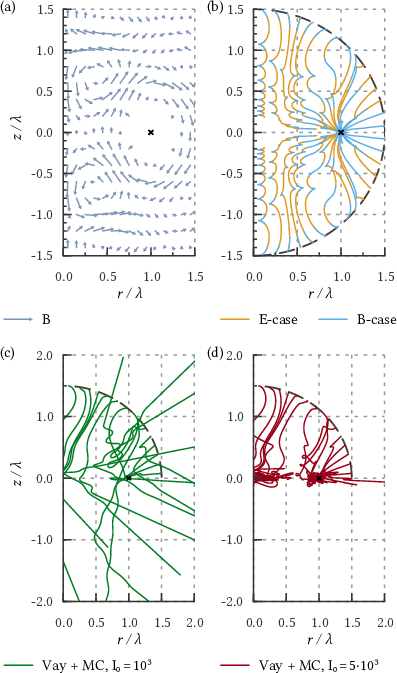
The field of a multipole harmonic wave that is completely absorbing by a current loop can be obtained by time reversal of the field emitting by a current loop (see App. B). The electron motion in the absorbing multipole wave with the angular frequency $\omega=2\pi c/\lambda$ for a loop radius $r_{\ell}=\lambda=1\;\mu\text{m}$ is shown in Fig. 4, where in the cylindrical coordinate system the ‘‘wire’’ position is marked with the black cross. The $z$ axis is the axis of the loop. Fig. 4 (a) demonstrates the magnetic field of the multipole wave at $t=0$ . Fig. 4 (b) shows the asymptotic electron trajectories, Figs. 4 (c) and (d) show the electron trajectories computed by Vay and MC algorithm for the loop current magnitude $I_{0}=1\times 10^{3}$ and for $I_{0}=5\times 10^{3}$ , respectively. The trajectories start at $t=0$ from the sphere shown by a thick dashed line and are computed up to $t=5\lambda/c$ .

It is seen from Fig. 4 that the current loop attracts the asymptotic electron trajectories. However, it is seen that the absorption-induced trapping is not really a strict trapping but just means that electrons in the radiation-dominated regime stay for a long time in the region with the currents absorbing the incoming waves.

VI Emission-absorption symmetry and general properties of asymptotic trajectories

In this section we consider the properties of the electron trajectories described by Eqs. (14) and (15). For this purpose let us consider the well-known symmetry of the Maxwell’s equations, namely, the following transform

	$\displaystyle t^{*}=-t,$		(27)
	$\displaystyle\mathbf{E^{*}=-E},$		(28)
	$\displaystyle\mathbf{B^{*}=B},$		(29)
	$\displaystyle\rho^{}=-\rho,\qquad\mathbf{j^{}=j}.$		(30)

does not change them, i.e. they leads to the Maxwell’s equations for the starred variables; here $\rho$ is the charge density and $\mathbf{j}$ is the current density. From here on we denote $\mathbf{E}$ , $\mathbf{B}$ , $\mathbf{j}$ evolving in time $t$ as initial system and $\mathbf{E}^{*}$ , $\mathbf{B}^{*}$ , $\mathbf{j}^{*}$ evolving in time $t^{*}$ as starred system. This symmetry is the relation between a system of currents emitting some fields and the system of currents absorbing the fields: namely, the Poynting vector, the $\mathbf{j\cdot E}$ product and the time direction in the starred system is opposite to that in the initial system.

According to Eq. (15), in the starred system the velocity field $\mathbf{v}^{*}$ relates to the velocity field of the initial system $\mathbf{v}$ as follows:

\mathbf{v}^{*}(\mathbf{r},t^{*})=-\mathbf{v(\mathbf{r},-t^{*})},

(31)

that obeys the stability condition $\mathbf{v^{*}\cdot E^{*}}<0$ . Thus, in the starred system the velocity field and the time direction are opposite to that in the initial system, that leads to the same trajectories in the starred system $\mathbf{r}^{*}(t^{*})$ as in the initial system, passed by the electrons in the opposite direction: $d\mathbf{r}^{*}/dt^{*}=\mathbf{v}^{*}(\mathbf{r}^{*},t^{*})=-\mathbf{v}(\mathbf{r}^{*},-t^{*})$ .

Let us note a fundamental difference between the asymptotic trajectories described by Eqs. (15), (14), and by the ponderomotive description. The ponderomotive force is determined by the distribution of $E^{2}$ and $B^{2}$ and is indifferent to the transform Eqs. (27)–(30), whereas this transform reverses the direction of the electron motion in the case when Eqs. (15) and (14) are applicable, namely, when radiation reaction is strong.

In order to illustrate the difference between the ponderomotive description and the description by the velocity field Eq. (15) the following toy example can be considered. The first laser pulse propagates along the direction $\mathbf{x}_{0}$ and scatters an electron aside. Then the second pulse is formed from the first one with the substitution (28)–(29), and according to the Maxwell’s equations this pulse travels in the direction $-\mathbf{x}_{0}$ . In the framework of the ponderomotive description the second laser pulse is not important because it will never meet the electron scattered by the first pulse. At the same time, considering the first laser pulse as the initial system of fields, we see that the second laser pulse is equivalent to the starred system of fields. In the case of strong radiation reaction the asymptotic approach is valid, and the electron according to Eq. (31) will pass along its preceding trajectory in the opposite direction in the field of the second pulse, i.e. the electron will be brought back to its initial position by the second laser pulse.

Therefore, the asymptotic description of the electron motion Eqs. (14) and (15) implies that the electrons are not scattered by, but stay for a long time in the field of a laser pulse or in a laser beam. This conclusion is in a good agreement with the results of theoretical considerations and numerical simulations showing that the ponderomotive force can be significantly suppressed by the radiation reaction [34, 50].

VI.1 Asymptotic trajectories in standing waves

We see in Sec. IV that the reduced equations lead to periodic electron trajectories in the linearly polarized standing electromagnetic wave. Here we show, that Eqs. (14) and (15) always lead to a periodic electron trajectories in a wide class of fields, namely in the periodic fields which can be represented in the following form:

	$\displaystyle\mathbf{E}=\mathbf{f}(\mathbf{r},t)-\mathbf{f}(\mathbf{r},-t),$		(32)
	$\displaystyle\mathbf{B}=\mathbf{g}(\mathbf{r},t)+\mathbf{g}(\mathbf{r},-t),$		(33)

where $\mathbf{E=f}(\mathbf{r},t)$ , $\mathbf{B=g}(\mathbf{r},t)$ is the solution of Maxwell’s equations for some charge density $\rho$ and current density $\mathbf{j}$ (for the sake of simplicity let us consider $\rho=0$ and $\mathbf{j}=0$ ). This representation means that the fields are the sum of the fields of some system and the fields of the corresponding starred system. In this case the symmetry (27)–(30) leads to the same fields of the starred system as in the initial system, i.e. $\mathbf{E}^{*}(\mathbf{r},t^{*})=\mathbf{E}(\mathbf{r},t^{*})$ , $\mathbf{B}^{*}(\mathbf{r},t^{*})=\mathbf{B}(\mathbf{r},t^{*})$ , hence it should lead to the same velocity field $\mathbf{v}^{*}(\mathbf{r},t^{*})=\mathbf{v}(\mathbf{r},t^{*})$ , that together with Eq. (31) yields

\mathbf{v}(\mathbf{r},-t)=-\mathbf{v(\mathbf{r},t)}.

(34)

Thus, the velocity field in the electromagnetic fields (32)–(33) is an odd function of time. Consequently, the time reversal conserves the equation for the electron position,

\frac{d\mathbf{r}}{d(-t)}=\mathbf{v}(\mathbf{r},(-t)),

(35)

and the electron position $\mathbf{r}(t)$ is an even function of time. Therefore,

\mathbf{r}(t)-\mathbf{r}(-t)=\int_{-t}^{t}\mathbf{v}(\mathbf{r}(t),t)\,dt=\\ \int_{0}^{t}\mathbf{v}(\mathbf{r}(t),t)\,dt+\int_{0}^{t}\mathbf{v}(\mathbf{r}(-t),-t)\,dt=0.

(36)

As far as the velocity field governed by Eqs. (8) and (10)–(13) is a single-valued function of the electromagnetic fields, and the fields are periodic in time, the velocity field is also periodic with the same period, $T$ . Thus, the velocity field is an odd function relative to any time instant $t=nT$ , where $n$ is an integer. Let the electron starts to move at $t=nT-T/2$ , then it comes to the starting point a period later, $\mathbf{r}(nT+T/2)=\mathbf{r}(nT-T/2)$ , then due to the periodicity of $\mathbf{v}$ at $t=(n+1)T$ , we have $\mathbf{r}((n+1)T+T/2)=\mathbf{r}(nT+T/2)$ . Therefore, in the framework of the asymptotic approach, the electron is moving periodically back and forth along the same path in the periodic fields Eqs. (32)–(33).

VI.2 Asymptotic trajectories in a laser beam of finite diameter

Here we stress that many field configurations could be reduced to the form of periodic fields that obey the emission-absorption symmetry Eqs. (27)–(30). In the previous subsection we also assumed that the velocity field is a single-valued function of the fields. This is not strictly true in the B-case, because one can add to $\mathbf{v}$ from Eq. (8) a vector parallel to $\mathbf{B}$ . The effect of this ambiguity is also discussed in this section.

Let us consider the fields of TE11 mode of a rectangular metallic waveguide:

	$\displaystyle E_{x}=0,$		(37)
	$\displaystyle E_{y}=a_{0}\cos(k_{y}y)\sin(k_{z}z)\cos(t-k_{x}x),$		(38)
	$\displaystyle E_{z}=-\frac{a_{0}k_{y}}{k_{z}}\sin(k_{y}y)\cos(k_{z}z)\cos(t-k_{x}x),$		(39)
	$\displaystyle B_{x}=\frac{a_{0}(k_{z}^{2}+k_{y}^{2})}{k_{z}}\cos(k_{y}y)\cos(k_{z}z)\sin(t-k_{x}x),$		(40)
	$\displaystyle B_{y}=-k_{x}E_{z},$		(41)
	$\displaystyle B_{z}=k_{x}E_{y},$		(42)

where we assume that the wave angular frequency $\Omega=(k_{x}^{2}+k_{y}^{2}+k_{z}^{2})^{1/2}=1$ (here we use the normalization frequency $\omega$ equal to the frequency of the wave, and, as before, the time is normalized to $1/\omega$ , coordinates are normalized to $c/\omega$ , $\mathbf{k}$ is the wavenumber normalized to $\omega/c$ ). These fields obey the metallic boundary conditions at $y=0,\;\pm\ell_{y},\;\pm 2\ell_{y},...$ ( $E_{z}=0$ ) and at $z=0,\;\pm\ell_{z},\;\pm 2\ell_{z},...$ ( $E_{y}=0$ ). Here $\ell_{y}=\pi/k_{y}$ and $\ell_{z}=\pi/k_{z}$ are the sizes of the waveguide along the $y$ - and $z$ -axes, respectively.

The fields Eqs. (37)–(42) are the solution of the Maxwell’s equations not only inside the waveguide but in the open space as well because this fields can be represented as a sum of plane waves. Particularly, we consider these fields in the region $y\in[-\ell_{y}/2,\ell_{y}/2]$ and $z\in[0,\ell_{z}]$ as the model of the laser beam of finite diameter. If $\ell_{y}\gg\ell_{z}$ , the electric field is mainly directed along the $y$ -axis and reaches its maximum in the center of the beam.

The fields Eqs. (37)–(42) are shown in Fig. 5 (a) for $\ell_{y}=4\pi$ , $\ell_{z}=2\pi$ and $t=x=0$ . The asymptotic electron trajectory computed for these fields is shown in Fig. 5 (b), where $\xi=x-v_{g}t$ , $v_{g}=k_{x}\approx 0.83$ is the group velocity of the electromagnetic wave, and the trajectory starts at $t=0$ , $x=0$ , $y=0.2$ and $z=0.65$ and is computed up to $t=2\tau$ , where

\tau=\frac{2\pi}{k_{x}(v_{\phi}-v_{g})}=\frac{2\pi}{1-k_{x}^{2}}

(43)

is the intrinsic timescale of the task, $v_{\phi}=1/v_{g}$ is the phase velocity of the wave. For Fig. 5 $c\tau/\lambda\approx 3.2$ . In Figs. 5 (c) and (d) the same asymptotic trajectory is shown as the thick blue line. Five electron trajectories in the fields given by Eqs. (37)-(42) are shown in Figs. 5 (c) and (d). These trajectories start at the same point as the asymptotic trajectory, but they are computed by Vay’s algorithm with quantum radiation reaction incorporated by Monte Carlo technique. For Figs. 5 (c) and (d) we use $a_{0}=700$ and $a_{0}=4\times 10^{3}$ , respectively.

It is seen from Figs. 5 (b), (c) and (d) that the asymptotic trajectory is quasiperiodic, that is in a qualitative agreement with the fact that for $a_{0}=4\times 10^{3}$ the electrons stay for a long time in the high-field region. However, as we see below, the asymptotic trajectories being computed in the laboratory reference frame yield the values of $\xi$ and the values of the trajectory period which do not coincide well with that for real electron trajectories. The reason for that is that Eq. (8) is not Lorentz invariant, namely if one compute $\mathbf{v}$ from it in some reference frame, in another reference frame he obtain ${\mathbf{v}^{\prime}=E^{\prime}\times B^{\prime}+aB^{\prime}}$ , where $a$ is a constant.

Let us transform the fields Eqs. (37)–(42) to the reference frame $K^{\prime}$ moving along the $x$ axis with the group velocity of the fields $v_{g}$ . This lead to the following fields:

	$\displaystyle E_{y}^{\prime}=a_{0}k_{\perp}\cos(k_{y}y)\sin(k_{z}z)\cos(k_{\perp}t^{\prime}),$		(44)
	$\displaystyle E_{z}^{\prime}=-\frac{a_{0}k_{\perp}k_{y}}{k_{z}}\sin(k_{y}y)\cos(k_{z}z)\cos(k_{\perp}t^{\prime}),$		(45)
	$\displaystyle B_{x}^{\prime}=\frac{a_{0}(k_{z}^{2}+k_{y}^{2})}{k_{z}}\cos(k_{y}y)\cos(k_{z}z)\sin(k_{\perp}t^{\prime}),$		(46)
	$\displaystyle E_{x}^{\prime}=B_{x}^{\prime}=B_{y}^{\prime}=B_{z}^{\prime}=0,$		(47)

where $k_{\perp}=\sqrt{1-k_{x}^{2}}$ . These fields do not depend on $x^{\prime}$ and for all the electrons in these fields the component of the Lorentz force along the $x^{\prime}$ axis is absent. Furthermore, the electrons due to the radiation reaction ‘‘forget’’ their initial direction of motion, hence we conclude that the average velocity of the electrons in the fields Eqs. (44)–(47) is $v_{x}^{\prime}=0$ . Therefore, in $K$ the average electron velocity is $v_{x}=v_{g}$ hence $\xi=\operatorname{const}$ that is in good agreement with results of Vay+MC simulations. Note that $\xi=\operatorname{const}$ does not coincide with the result of the asymptotic consideration in the laboratory reference frame (see Fig. 5 (b)). Also, a wrong value of $v_{x}$ leads to a wrong value of the period of $y$ and $z$ coordinates of the electron in the framework of the asymptotic approach.

The substitution $t^{\prime}\rightarrow t^{\prime}+\pi/2k_{\perp}$ yields that the electric field given by Eqs. (44)–(45) are odd functions of time and the magnetic field Eq. (46) is the even function of time in $K^{\prime}$ . As follows from Sec. VI.1 in this case the electron trajectories are periodic in the radiation-dominated regime and their period is equal to $2\pi/k_{\perp}$ in $K^{\prime}$ . Therefore, in the laboratory reference frame in the radiation-dominated regime the electrons move along the $x$ -axis with the group velocity of the laser beam, and, as $y^{\prime}=y$ and $z^{\prime}=z$ , the electron trajectories are periodic in the $yz$ plane with the period

\frac{2\pi}{k_{\perp}\sqrt{1-v_{g}^{2}}}=\tau.

(48)

Thus, the ambiguity of the velocity field in the asymptotic approach can be resolved by appropriate choose of the reference frame.

Therefore, we show that the asymptotic description, Eqs. (14) and (15), leads to periodic trajectories in a wide class of standing waves (e.g. formed by laser beams of finite diameter), and to electron motion along the laser beam with its group velocity with periodic transverse motion. The latter may explain the effect of the radiation-reaction trapping [50].

VII Conclusion

To conclude, here we show that in the radiation-dominated regime the electrons tend to move with velocity that is determined by the fields only, see Eq. (15). This means that the electron trajectory can be found from the first-order equation, Eq. (14). We call this velocity asymptotic because it can be found as the asymptotic electron velocity ( $t\to\infty$ ) in the constant field approximation. The reason for reduction of the equation order is that the electron energy in the radiation-dominated regime is small ( $\gamma\ll a_{0}$ ), the electrons are ‘‘light’’ and are easily turned by the laser field to the asymptotic direction in a time much smaller than the characteristic variation time of the electromagnetic fields. The velocity field ${\mathbf{v}}({\mathbf{r}},t)$ corresponds to the absence of the component of the Lorentz force transverse to the electron velocity, so $\mathbf{v}$ is also called the radiation-free direction [35].

In a number of the electromagnetic field configurations we found the numerical solutions of the reduced-order equations and the full equations of electron motion with the radiation reaction taken into account by the Monte Carlo technique and the Baier–Katkov synchrotron formulae [43]. The comparison between these solutions demonstrates that the reduced-order equations can be used for a qualitative description of the electron trajectories for $a_{0}$ greater or of the order of thousand for optical wavelengths. In order to stress these high values of $a_{0}$ we call the solutions of the reduced equations of motion as asymptotic trajectories ( $a_{0}\to\infty$ ).

Also we demonstrate that the reduced-order equations for the electron trajectories in the radiation-dominated regime are the useful analytical tool. First, they predict the electron trapping in the regions where the wave field is absorbed, see Sec. V. This result can be important for the theoretical consideration of the field absorption by the QED cascade in the counter-propagating laser waves [18]. Second, contrary to the concept of the ponderomotive force, the asymptotic theory leads to periodic electron trajectories in a wide class of standing electromagnetic fields (including the case of counter-propagating tightly focused laser beams, see Sec. VI.1). This result is in a good agreement with Ref. [34] that demonstrates the reduction of the ponderomotive force in the radiation-dominated regime. Furthermore, using a certain configuration of the laser beam we demonstrate that the beam in the radiation-dominated regime does not push the electrons aside, but captures and carries them with the group velocity of the beam. This result probably explains the radiation-reaction trapping observed in the numerical simulation of Ref. [50].

Therefore, the concept of the ponderomotive force is not applicable in the radiation-dominated regime and can be replaced by the description of the asymptotic electron trajectories. This concept implies that velocities of the electrons in a given point are the same hence the electrons (positrons) in the radiation-dominated regime can be described in the framework of the hydrodynamical approach. The Maxwell’s equations, in which the electron current is determined only by the plasma density and by the local field values (see Eq. (15)), together with the continuity equation for the plasma density are formed the closed system of equations. Note that the reduced-order equations gives the positive field work on the electrons ( ${\mathbf{v}\cdot E}<0$ ) hence the plasma in the framework of the asymptotic theory is always an absorbing medium. In more details this hydrodynamical approach will be considered elsewhere.

Acknowledgements.

We thank A. V. Bashinov and V. A. Kostin for fruitful discussions. We are grateful to E. V. Frenkel who brought our attention to the symmetries of the Maxwell’s equations, and to T. Docker for his help with haskell-chart library. This research was supported by the Grants Council under the President of the Russian Federation (Grant No. MK-2218.2017.2). The study of the absorption-induced trapping was supported by the Russian Science Foundation through Grant No. 16–12-10383

Appendix A Tests of numerical instruments

A.1 Radiation reaction: classical limit

In order to test the Vay’s solver for the equations of motion [46] coupled with Landau–Lifshitz radiation reaction force (taken into account by Euler method) let us consider electron motion in constant crossed electric and magnetic fields:

	$\displaystyle E_{y}=a_{0}/2,\quad B_{z}=a_{0},$		(49)
	$\displaystyle E_{x}=E_{z}=B_{x}=B_{y}=0.$		(50)

In the reference frame $K^{\prime}$ moving along $x$ axis with the speed $V=0.5$ the electric field vanishes and the only $z$ component of the magnetic field remains: $B_{z}^{\prime}=B_{z}\sqrt{1-V^{2}}$ , where the stroke marks quantities in $K^{\prime}$ . Taking into account the Landau–Lifshitz radiation reaction, for relativistic electron motion in $K^{\prime}$ we obtain (assuming $\gamma\gg 1$ ):

	$\displaystyle d\gamma^{\prime}/dt^{\prime}=-C\gamma^{\prime 2},$		(51)
	$\displaystyle dw^{\prime}/dt^{\prime}=iB_{z}^{\prime}w^{\prime}/\gamma^{\prime},$		(52)
	$\displaystyle dv_{z}^{\prime}/dt^{\prime}=0,$		(53)

where

C=\frac{2}{3}\frac{e^{2}}{\hbar c}\frac{\hbar\omega}{mc^{2}}B_{z}^{\prime 2}v_{\perp}^{2},

(54)

$w^{\prime}=v_{x}^{\prime}+iv_{y}^{\prime}$ , $v_{\perp}^{2}=v_{x}^{\prime 2}+v_{y}^{\prime 2}$ and $\omega$ is just some frequency used for normalization of time. The solution of Eqs. (51)-(53) is the following:

	$\displaystyle\gamma^{\prime}=\frac{\gamma_{0}^{\prime}}{1+\gamma_{0}^{\prime}Ct^{\prime}},$		(55)
	$\displaystyle w^{\prime}=w_{0}^{\prime}\exp\left(\frac{iB_{z}^{\prime}}{\gamma_{0}^{\prime}}(t^{\prime}+\frac{\gamma_{0}Ct^{\prime 2}}{2})\right),$		(56)

and

x^{\prime}+iy^{\prime}=x_{0}^{\prime}+iy_{0}^{\prime}+w_{0}^{\prime}\sqrt{\frac{i\pi}{2B_{z}^{\prime}C}}\exp\left(-\frac{iB_{z}^{\prime}}{2\gamma_{0}^{\prime 2}C}\right)\\ \times\left\{\operatorname{erf}\left(\sqrt{\frac{B_{z}^{\prime}C}{2i}}(t^{\prime}+\frac{1}{\gamma_{0}^{\prime}C})\right)\right.\\ \left.-\operatorname{erf}\left(\sqrt{\frac{B_{z}^{\prime}C}{2i}}\frac{1}{\gamma_{0}^{\prime}C}\right)\right\},

(57)

where subscript $0$ denotes $t^{\prime}=0$ and

\operatorname{erf}(x)=\frac{2}{\sqrt{\pi}}\int_{0}^{x}\exp(-t^{2})\,dt

(58)

is the error function.

Figure 6 (a) demonstrates the electron trajectory in the $xy$ plane obtained with the numerical integration of the equation of motion taking into account radiation reaction in Landau–Lifshitz form (solid blue line) for $a_{0}=50.3$ , $\omega=2\pi c/\lambda$ , $\lambda=1.1\text{ nm}$ , $x_{0}=y_{0}=0$ , $v_{x}(t=0)\simeq 0.8$ , $v_{z}(t=0)\simeq 0.6$ and $\gamma_{0}=63$ . Note that these parameters ensure $v_{\perp}^{\prime}(t)=v_{x}^{\prime}(t=0)=0.5=V$ , leading in the laboratory reference frame to the cycloid-like trajectory with points of $dy/dx\rightarrow\infty$ .

For the given parameters we obtain $B^{\prime}_{z}=43.6$ , $\gamma_{0}^{\prime}=\gamma^{\prime}(t^{\prime}=0)=43.6$ and $C=4.9\times 10^{-3}$ , and from Eq. (55) at the time instant $t_{1}^{\prime}=6\pi$ we get $\gamma^{\prime}(t_{1}^{\prime})=\gamma_{0}^{\prime}/5$ . Neglecting displacement of the particle, $x^{\prime}$ , and assuming $v_{x}^{\prime}(t_{1}^{\prime})=V$ , we finally get for the laboratory reference frame: $t_{1}=(1-V^{2})^{-1/2}t_{1}^{\prime}\approx 22$ and $\gamma(t_{1})\approx 12.6$ . It should be mentioned that at the time instance at which $v_{x}^{\prime}=V$ , in the laboratory reference frame the Lorentz factor reaches its local maximum. Numerical solver using Landau–Lifshitz force demonstrates that the local maximum of $\gamma$ closest to $t_{1}=22$ is reached at $t\approx 21.5$ and is $\gamma\approx 13.4$ that is quite close to the predicted value.

Equation (57) yields $y^{\prime}(t^{\prime}\rightarrow\infty)\approx 0.463$ for the above-mentioned parameters. This value ( $y(t\rightarrow\infty)=y^{\prime}(t^{\prime}\rightarrow\infty)$ ) is depicted as gray dotted line in Fig. 6, and in a good agreement with the value obtained with the numerical solver. The dashed orange line is got by means of particle pusher that takes into account with the quantum formulae and is described in the next subsection.

A.2 Radiation reaction: general case

The quantum radiation reaction can be taken into account in Vay’s pusher by means of Monte Carlo technique. To do this we use the alternative event generator [44] based on Baier–Katkov synchrotron formula [37, 45]. The event generator checks at every time step if the photon emission occurs, and if it does, the electron momentum is decreased on the momentum of the emitted photon. Using of classical description of the electron trajectory together with the quantum formula for the photon emission is valid because the radiation formation length in strong fields ( $a_{0}\gg 1$ ) is much smaller than the field characteristic scale [37, 45, 51].

In order to test Vay’s pusher coupled with Monte Carlo event generator we compute the energy distribution of the electrons in the crossed fields Eqs. (49)–(50). The resulting spectra are compared with the spectra obtained from the Boltzmann equation in the reference frame $K^{\prime}$ .

As mentioned above, in the reference frame $K^{\prime}$ moving along $x$ axis with velocity $V=0.5$ the electrons see the pure magnetic field directed along the $z$ axis. Therefore, in $K^{\prime}$ the Boltzmann equation that describes the electron energy distribution $f^{\prime}(t^{\prime},\gamma^{\prime})$ is the following:

\frac{\partial f^{\prime}(t^{\prime},\gamma^{\prime})}{\partial t^{\prime}}=\int_{\gamma^{\prime}}^{\infty}w(\epsilon,\epsilon-\gamma^{\prime})f^{\prime}(t^{\prime},\epsilon)\,d\epsilon\\ -W(\gamma^{\prime})f^{\prime}(t^{\prime},\gamma^{\prime}),

(59)

where

w(\epsilon,\epsilon_{\gamma})=-\frac{\alpha}{\epsilon_{\ell}\epsilon^{2}}\left[\int_{\varkappa}^{\infty}\operatorname{Ai}(\xi)\,d\xi\right.\\ \left.+\left(\frac{2}{\varkappa}+\frac{\epsilon_{\gamma}\chi\varkappa^{1/2}}{\epsilon}\right)\operatorname{Ai}^{\prime}(\varkappa)\right],

(60)

is the distribution of the photon emission probability by the electron with the Lorentz factor $\epsilon$ over the photon energy $\varepsilon_{\gamma}$ normalized to $mc^{2}$ , i.e. over $\epsilon_{\gamma}=\varepsilon_{\gamma}/mc^{2}$ (see Refs. [37, 45]), and

	$\displaystyle\chi=\epsilon_{\ell}B_{z}^{\prime}v_{\perp}\epsilon,$		(61)
	$\displaystyle\varkappa=\left[\frac{\epsilon_{\gamma}}{(\epsilon-\epsilon_{\gamma})\chi}\right]^{2/3},$		(62)
	$\displaystyle W(\gamma^{\prime})=\int_{0}^{\gamma^{\prime}}w(\gamma^{\prime},\epsilon_{\gamma})\,d\epsilon_{\gamma}$		(63)

is the overall emission probability for an electron with the Lorentz factor $\gamma^{\prime}$ , $\epsilon_{\ell}=\hbar\omega/mc^{2}$ , $\omega$ is the frequency used for normalization of time.

The Boltzmann equation (59) can be solved numerically as follows. In finite-difference method the distribution function $f^{\prime}(\gamma^{\prime})$ is represented as a vector, and the right-hand-side of the Eq. (59) is represented as the product of a matrix and a vector. Then Euler method can be used, and the computation of $f^{\prime}(t^{\prime},\gamma^{\prime})$ from $f^{\prime}(t^{\prime}=0,\gamma^{\prime})$ is reduced to a matrix exponentiation, that can be done with square-and-multiply algorithm that have logarithmic complexity on the number of time steps. Then the distribution function in the initial reference frame can be found from $f^{\prime}(t^{\prime},\gamma^{\prime})$ with Lorentz transformation. For that one should neglect the electron displacement in $K^{\prime}$ (i.e., $x^{\prime}(t^{\prime})-x^{\prime}(0)$ ) and assume that in $K^{\prime}$ the angles $\varphi^{\prime}$ between $x^{\prime}$ axis and ${\mathbf{v}}_{\perp}^{\prime}$ are uniformly distributed on the interval $[0,2\pi)$ :

	$\displaystyle t=t^{\prime}\Gamma,$		(64)
	$\displaystyle\gamma=\gamma^{\prime}\Gamma(1+Vv_{\perp}\cos\varphi^{\prime}),$		(65)

f(\gamma)\propto\int f^{\prime}(\gamma^{\prime})\frac{d\gamma^{\prime}}{d\gamma}\,d\varphi^{\prime}\\ =\int\frac{f^{\prime}(\gamma^{\prime})}{(1+Vv_{\perp}\cos\varphi^{\prime})}\,d\varphi^{\prime},

(66)

where the integration should be performed over the path determined by the value of $\gamma$ and Eq. (65); $\Gamma=(1-V^{2})^{-1/2}$ . It is worth noting that for correctness of the method the step along $\gamma^{\prime}$ in the finite-difference scheme should be much smaller than the width of the emission spectrum. Thus, especially small step of $\gamma^{\prime}$ should by used in the classical regime.

Figure 6 (b) demonstrates the electron spectra in the crossed fields Eq. (49)-(50) with $a_{0}=50.3$ and $\lambda=1.1\text{ nm}$ used for the normalization. The electrons initially (at $t=0$ ) move along $x$ and $z$ axes ( $v_{x}\simeq 0.8$ , $v_{z}\simeq 0.6$ ) and have Lorentz factor $\gamma_{0}=63$ . Curves A and C are obtained by Eq. (59) for $t=22$ and $t=49.5$ , respectively. Curves B and D represent the spectra of $8000$ particles whose trajectory is computed by Vay’s pusher coupled with Monte Carlo event generator, for $t=22$ and $t=49.5$ , respectively.

In $K^{\prime}$ the parameters of the simulations yield the quantum parameter $\chi^{\prime}(t^{\prime}=0)=2$ , and if Landau–Lifshitz radiation reaction is used, $\chi^{\prime}$ drops down to $\chi^{\prime}(t=22)=0.4$ and $\chi^{\prime}(t=49.5)=0.1$ (see Eq. (55)). However, initially $\chi^{\prime}\gtrsim 1$ that leads to wide emission spectrum and wide resulting spectrum of the electrons. Moreover, the overall emission probability is not very high and a significant fraction of electrons do not emit photons at all. These electron fractions form peaks clearly seen on the curves A and B. The position of the peak on the curve A corresponds to non-emitting electrons with $v_{x}^{\prime}=-0.5$ that according to Eq. (65) gives $\gamma\approx 38$ . However, in Monte Carlo simulation at $t=22$ the distribution of electrons over $\varphi^{\prime}$ is far from the uniform one, and most of the non-emitting electrons moves with $v_{x}\approx 0.5$ leading to the peak at $\gamma=\gamma(t=0)$ . Thus, the difference of curves A and B comes from the assumption of uniform electron distribution over the angle $\varphi^{\prime}$ . This assumption becomes more reliable at later times ( $t=49.5$ ), and the difference between two methods of the spectra computation vanishes (see curves C and D).

Therefore, the results of the Vay’s pusher coupled with the Landau–Lifshitz radiation reaction force or with the Monte Carlo event generator (that uses some approximate expression for fast computation of the emission probability) coincides well with the results obtained by other methods.

Appendix B Multipole wave

In the cylindrical coordinates the vector potential $\mathbf{A}$ of the current loop obeys the following equation:

\Delta A_{\varphi}-\partial_{t}^{2}A_{\varphi}=-j_{\varphi},

(67)

where we assume that the $z$ -axis is the axis of the loop, thus $A_{r}=A_{z}=0$ . The solution of this equation for the harmonic current $j_{\varphi}\propto\exp(-i\omega t)$ (obviously, in the normalized units $\omega=1$ ) can be found using Green’s function as follows [52]:

A_{\varphi}=-\frac{I_{0}r_{\ell}}{\pi\bar{z}}\int_{0}^{\pi/2}\frac{\cos(2\psi)}{s}\exp(-it+is\bar{z})\,d\psi,

(68)

where $I_{0}$ is the current amplitude, $\bar{z}=[z^{2}+(r+r_{\ell})^{2}]^{1/2}$ , $s=(1-\kappa\sin^{2}\psi)^{1/2}$ and $\kappa=4rr_{\ell}/{\bar{z}}^{2}$ . Then the electric and magnetic fields can be found from the Eq. (68).

To obtain the field of a multipole wave that is fully absorbed by the current loop, the substitution $t\to-t$ , $B\to-B$ is made. Then the fields are computed on the $r-z$ lattice, and their values are used for the interpolation in the numerical solution of the equations of the electron motion.

References

[1] S. V. Bulanov, T. Z. Esirkepov, J. Koga, and T. Tajima, Plasma Physics Reports 30, 196 (2004).
[2] A. Di Piazza, K. Z. Hatsagortsyan, and C. H. Keitel, Physical Review Letters 102, 254802 (2009).
[3] R. Duclous, J. G. Kirk, and A. R. Bell, Plasma Physics and Controlled Fusion 53, 015009 (2011).
[4] E. N. Nerush and I. Y. Kostyukov, Nuclear Instruments and Methods in Physics Research A 653, 7 (2011).
[5] A. G. R. Thomas, C. P. Ridgers, S. S. Bulanov, B. J. Griffin, and S. P. D. Mangles, Physical Review X 2, 41004 (2012).
[6] N. Neitz and A. Di Piazza, Phys. Rev. Lett. 111, 054802 (2013).
[7] M. Vranic, T. Grismayer, R. A. Fonseca, and L. O. Silva, New Journal of Physics 18, 073035 (2016).
[8] Cole, Behm, Ilderton, Sarri, Ridgers, and Mangles, (2017).
[9] K. Poder, M. Tamburini, G. Sarri, and A. e. a. Di Piazza, (2017).
[10] S. Corde, K. Ta Phuoc, G. Lambert, R. Fitour, V. Malka, A. Rousse, A. Beck, and E. Lefebvre, Reviews of Modern Physics 85, 1 (2013).
[11] G. Sarri, D. J. Corvan, W. Schumaker, J. M. Cole, A. Di Piazza, H. Ahmed, C. Harvey, C. H. Keitel, K. Krushelnick, S. P. D. Mangles, Z. Najmudin, D. Symes, A. G. R. Thomas, M. Yeung, Z. Zhao, and M. Zepf, Physical Review Letters 113, 224801 (2014).
[12] W. Yan, C. Fruhling, G. Golovin, D. Haden, J. Luo, P. Zhang, B. Zhao, J. Zhang, C. Liu, M. Chen, and S. Chen, Nature Photonics 11, 514 (2017).
[13] C. P. Ridgers, C. S. Brady, R. Duclous, J. G. Kirk, K. Bennett, T. D. Arber, A. P. L. Robinson, and A. R. Bell, Phys. Rev. Lett. 108, 165006 (2012).
[14] A. V. Bashinov and A. V. Kim, Physics of Plasmas 20, 113111 (2013).
[15] E. N. Nerush, I. Y. Kostyukov, L. Ji, and A. Pukhov, Physics of Plasmas 21, 013109 (2014).
[16] L. L. Ji, A. Pukhov, E. N. Nerush, I. Y. Kostyukov, B. F. Shen, and K. U. Akli, Physics of Plasmas 21, 023109 (2014a), 10.1063/1.4866014.
[17] H.-Z. Li, T.-P. Yu, J.-J. Liu, Y. Yin, X.-L. Zhu, R. Capdessus, F. Pegoraro, Z.-M. Sheng, P. McKenna, and F.-Q. Shao, Scientific Reports 7, 17312 (2017).
[18] E. N. Nerush, I. Y. Kostyukov, A. M. Fedotov, N. B. Narozhny, N. V. Elkina, and H. Ruhl, Phys. Rev. Lett. 106, 035001 (2011).
[19] A. Gonoskov, A. Bashinov, S. Bastrakov, E. Efimenko, A. Ilderton, A. Kim, M. Marklund, I. Meyerov, A. Muraviev, and A. Sergeev, Physical Review X 7, 041003 (2017).
[20] M. Tamburini, F. Pegoraro, A. D. Piazza, C. H. Keitel, and A. Macchi, New Journal of Physics 12, 123005 (2010).
[21] M. Tamburini, T. V. Liseykina, F. Pegoraro, and A. Macchi, Physical Review E 85, 016407 (2012).
[22] R. Capdessus, E. d’Humières, and V. T. Tikhonchuk, Physical Review E 86, 036401 (2012).
[23] R. Capdessus and P. McKenna, Physical Review E 91, 053105 (2015).
[24] E. N. Nerush and I. Y. Kostyukov, Plasma Physics and Controlled Fusion 57, 035007 (2015).
[25] E. G. Gelfer, A. M. Fedotov, and S. Weber, Plasma Physics and Controlled Fusion 60, 064005 (2018a).
[26] E. Gelfer, N. Elkina, and A. Fedotov, Scientific Reports 8, 6478 (2018b).
[27] T. Grismayer, M. Vranic, J. L. Martins, R. A. Fonseca, and L. O. Silva, Physics of Plasmas 23, 056706 (2016).
[28] P. Zhang, C. P. Ridgers, and A. G. R. Thomas, New Journal of Physics 17, 043051 (2015).
[29] T. V. Liseykina, S. V. Popruzhenko, and A. Macchi, New Journal of Physics 18, 072001 (2016).
[30] Y. B. Zel’dovich, Soviet Physics Uspekhi 18, 79 (1975).
[31] A. D. Piazza, Letters in Mathematical Physics 83, 305 (2008), 0801.1751v2 .
[32] I. Y. Kostyukov and E. N. Nerush, Physics of Plasmas, Volume 23, Issue 9, id.093119 23, 093119 (2016).
[33] M. A. Miller, Izu. vjssh. ucheb. Zaved. Radiofiz. 1, 110 (1958).
[34] A. M. Fedotov, N. V. Elkina, E. G. Gelfer, N. B. Narozhny, and H. Ruhl, Physical Review A 90, 053847 (2014).
[35] A. Gonoskov and M. Marklund, ‘‘Radiation dominated particle and plasma dynamics,’’ (2017), arXiv:physics.plasm-ph/1707.05749 .
[36] A. Gonoskov, A. Bashinov, I. Gonoskov, C. Harvey, A. Ilderton, A. Kim, M. Marklund, G. Mourou, and A. Sergeev, Physical Review Letters 113, 014801 (2014).
[37] L. D. Landau and E. M. Lifshitz, edited by T. C. T. of Fields (Elsevier, Oxford, 1975).
[38] B. Le Garrec, S. Sebban, D. Margarone, M. Precek, S. Weber, O. Klimo, G. Korn, and B. Rus, Proc. SPIE 8962, 8962 (2014).
[39] http://www.eli-np.ro/.
[40] https://portail.polytechnique.edu/luli/en/cilex-apollon/apollon.
[41] https://www.clf.stfc.ac.uk/Pages/Vulcan-2020.aspx.
[42] A. V. Bashinov, A. A. Gonoskov, A. V. Kim, G. Mourou, and A. M. Sergeev, The European Physical Journal Special Topics 223, 1105 (2014).
[43] V. B. Berestetskii, E. M. Lifshitz, and L. P. Pitaevskii, Quantum Electrodynamics (Pergamon, New York, 1982).
[44] N. V. Elkina, A. M. Fedotov, I. Y. Kostyukov, M. V. Legkov, N. B. Narozhny, E. N. Nerush, and H. Ruhl, Physical Review Special Topics - Accelerators and Beams 14, 054401 (2011).
[45] V. N. Baier, V. Katkov, and V. Strakhovenko, Electromagnetic processes at high energies in oriented single crystals (World Scientific, Singapore, 1998).
[46] J.-L. Vay, Physics of Plasmas 15, 056701 (2008).
[47] http://iapras.ru/english/structure/dep_330/quill.html.
[48] E. N. Nerush, D. A. Serebryakov, and I. Y. Kostyukov, The Astrophysical Journal 851, 129 (2017).
[49] A. V. Bashinov, P. Kumar, and A. V. Kim, Physical Review A 95, 042127 (2017).
[50] L. L. Ji, A. Pukhov, I. Y. Kostyukov, B. F. Shen, and K. Akli, Phys. Rev. Lett. 112, 145003 (2014b).
[51] A. Gonoskov, S. Bastrakov, E. Efimenko, A. Ilderton, M. Marklund, I. Meyerov, A. Muraviev, A. Sergeev, I. Surmin, and E. Wallin, Phys Rev E Stat Nonlin Soft Matter Phys 92, 023305 (2015).
[52] J. D. Jackson, Classical Electrodynamics, 3rd ed. (John Wiley & Sons, New York, 1999).