PyUltraLight: A Pseudo-Spectral Solver for Ultralight Dark Matter Dynamics
Abstract
PyUltraLight simulates the dynamics of ultralight dark matter in a non-expanding background. PyUltraLight can describe the evolution of several interacting ultralight dark matter halos or one or more halos orbiting a central, fixed Newtonian potential, the latter scenario corresponding to dwarf galaxies orbiting a massive central galaxy. We verify PyUltraLight by showing that it reproduces qualitative dynamical features of previously published simulations and demonstrate that it has excellent energy-conservation properties. PyUltraLight is implemented in a Python-based Jupyter notebook, solving the Schrödinger-Poisson equation governing ultralight scalar field dark matter dynamics in the non-relativistic regime using a symmetrised split-step pseudospectral algorithm. The notebook interface makes it simple to specify simulation parameters and visualise the resulting output but performance-critical routines are managed via calls to computationally efficient compiled libraries. PyUltraLight runs on standard desktop hardware with support for shared memory mutlithreading and is available on GitHub.
1 Introduction
The realisation that there may be more to the universe than meets the eye is one of the most profound developments in 20 Century astronomy and astrophysics. However, while there are now multiple lines of evidence that dark matter outweighs baryonic matter by a ratio of approximately 5:1 [1], we have few clues regarding the physical nature of dark matter. Much theoretical and experimental effort has focused on WIMP models, motivated by their consistency with supersymmetric extensions to the Standard Model and their relatively simple dynamics. However, advanced direct-detection experiments are putting increasingly tight constraints on the WIMP parameter space [2, 3] and CDM cosmology with simple, pressureless, noninteracting dark matter (a class including simple WIMP scenarios) is potentially at odds with observations at small astrophysical scales [4].
The potential shortcomings of simple cold dark matter scenarios motivate investigations of more novel dark matter scenarios. In particular, ultralight dark matter (ULDM), also known as fuzzy dark matter (FDM), or BEC dark matter, is an increasingly well-studied possibility; for a recent review of the potential advantages and characteristic attributes of this scenario see Ref [5]. ULDM models are well motivated by fundamental theories possessing approximate shift symmetries such as the theory of the QCD axion [6, 7]. Moreover, ULDM can naturally resolve the small-scale problems of CDM as the Heisenberg uncertainty principle suppresses gravitational collapse on length scales shorter than the de Broglie wavelength of the ULDM particle. In this regime the mass of the ULDM particle becomes correlated with astrophysical observables; if it is on the order of eV, structure is suppressed at kiloparsec scales and below [8].
Given the presence of a fundamental lengthscale, the behaviour of ULDM is more complex than that of simple dark matter scenarios whose cosmologically relevant interactions are purely gravitational. Physically, the effective short-scale pressure and condensate-like properties of ULDM create new dynamical possibilities for ULDM scenarios, such as purely pressure supported soliton-like solutions [9] and superposition or interference during interactions between condensate-like halos [10]. Consequently, modelling dark matter dynamics in ULDM scenarios is more challenging than in simple cold dark matter models, but is critical to understanding the physical consequences of ULDM models.
In the non-relativistic regime, the dynamics of ULDM can be reduced to the Schrödinger-Poisson system, where the complex variable describes the local density of ULDM quanta while the Poisson equation describes the local gravitational potential. Many approaches have been taken to this problem, including both modifications of existing cosmological simulation codes and the development of new codes specifically designed for ULDM systems. One widely used approach is the Madelung fluid formulation of the Schrödinger-Poisson system [11] which has a quantum pressure term that can be treated numerically in a variety of ways. In Ref. [12], the cosmological code gadget [13] is modified to treat the quantum pressure as an effective particle-particle interaction and the resulting code, axion-gadget is publicly available [14]. Ref. [15] modifies a non-public extension of gadget, p-gadget3 to treat the quantum pressure term via smoothed-particle hydrodynamics (SPH) routines. The SPH approach is also used in Ref. [16], while a particle-mesh approach was implemented in [17]. Nyx [18] was modified in [10] to study merging ULDM solitonic cores, Galacticus [19] was modified in [20] to study the effects of tidal stripping and dynamical friction on ULDM halos, arepo [21] was modified in [22] to study the core-mass relationship and turbulence characteristics of ULDM halos, and gamer [23, 24] was modified [25] to perform a detailed study of structure formation in ULDM cosmologies.
While a large number of public codes can solve conventional dark matter scenarios, axion-gadget is the only currently available solver for ULDM dynamics. This paper introduces PyUltraLight, a stand-alone Python-based pseudospectral Schrödinger-Poisson solver, and demonstrates that it reproduces many of the key findings of more complicated cosmological simulation codes within a desktop computing environment. We anticipate that as a publicly available resource, PyUltraLight will serve as a valuable cross-check on more complex implementations, serve as a basis for further development of such codes within the computational cosmology community, and facilitate explorations of ULDM dynamics.
PyUltraLight is based on a symmetrised-split-step (leapfrog) solver for the time evolution, and uses a pseudospectral Fourier algorithm to solve the Poisson equation for the gravitational potential at each step.11 1 A similar methodology was described in Ref. [26]; at the time of writing this code has not been released. Spectral methods are often used to solve the Poisson equation in large scale structure simulations, while the PSpectre code [27] provides a pseudospectral solver for the evolution of the inflaton and fields coupled to it during parametric resonance and preheating after inflation [28, 29, 30]. This algorithm has order accurate time integration steps and sub-percent level energy conservation, while the wavefunction normalisation is conserved to machine precision. As a pseudospectral code, linear differential operators are computed by direct multiplication in the Fourier domain, while non-linear terms are evaluated in position space. Consequently, PyUltraLight is free from noise associated with spatial derivatives computed via finite-differencing. There is a necessary computational cost associated with the Fourier and inverse Fourier transforms but these transforms are optimised in PyUltraLight through the use of the pyFFTW pythonic wrapper around the C-based FFTW subroutine library [31, 32]. As the FFTW libraries offer full parallelisation, PyUltraLight is currently designed to take advantage of multiple cores on a user PC or shared-memory environment. Full MPI compatibility has not yet been implemented as we have not found a need to run simulations in a distributed-memory cluster environment, however future releases may address this possibility.
This paper is organised as follows. We first provide a short review of ULDM physics, including a derivation of the Schrödinger-Poisson equations from the underlying scalar-field Lagrangian. We then describe their implementation in PyUltraLight, before moving on to describe testing and verification procedures applied to the code. We reproduce a selection of results from a variety of recent ULDM simulations and discuss the energy conservation and accuracy as a function of spatial resolution.
2 The Physics of ULDM
2.1 The Schrödinger-Poisson System
The existence of an extremely light scalar field, minimally coupled to gravity, is the central premise on which ULDM models are predicated. Within the ULDM framework, it is proposed that this scalar field exists as a Bose-Einstein condensate, described by a single wavefunction which is governed by the Schrödinger-Poisson coupled differential equations. We begin by deriving this system of equations as a non-relativistic weak-field limit of a more general theory. We start from the action functional for a scalar field, , minimally coupled to gravity and in the absence of self-interactions,
| (1) |
where we have taken but retain factors of at this stage. Applying the variational principle to this action yields the Euler-Lagrange equations
| (2) |
We evaluate equation 2 using linear perturbation theory, adopting the perturbed FRW metric in the Newtonian gauge:
| (3) |
To linear order in we obtain
| (4) |
where . At late times in an expanding universe, and it is sufficient to set and in equation 4. This is a good approximation even at relatively high redshifts, including the epochs of early structure formation. Alternatively, if we consider a non-expanding universe, these equalities are true by definition. In either case, we can remove the third term in equation 4. The resulting equation can then be analysed using WKB methods in the non-relativistic regime.22 2 For a detailed explication of the WKB approximation in the non-relativistic limit, see [33]. This allows us to write an ansatz solution for the field :
| (5) |
where is assumed to be slowly varying in the sense that , , , and . Since is sourced by , we also have that . Direct substitution of the ansatz solution into equation 4, discarding heavily suppressed terms, yields
| (6) |
We have thus shown that satisfies the Schrödinger equation in this limit, which is interpreted as the macroscopic wavefunction of a Bose-Einstein condensate. It follows that the particle number density of the condensate is given by , so its mass density is simply . The local gravitational potential thus satisfies the Poisson equation,
| (7) |
where is Newton’s gravitational constant. The coupled equations 6 and 7 together form the nonlinear Schrödinger-Poisson system which describes the dynamics of ULDM in the non-relativistic regime. While Equations 6 and 7 are valid for open boundary conditions, PyUltraLight is designed to solve the Schrödinger-Poisson system under periodic boundary conditions. In this case the correct form of equation 7 is
| (8) |
where we subtract the average density from the right hand side of the Poisson equation. The form of Equation 8 is a consequence of Gauss’ law and the fact that the surface integral of the gradient of the field around the perimeter of the simulation grid is identically zero when periodic boundary conditions are imposed [34].
2.2 Field Rescalings
It is helpful to recast the Schrödinger-Poisson system (equations 6 and 7) in terms of adimensional quantities. In keeping with Refs [35, 26] we introduce length, time, and mass scales as follows:
| (9) | ||||
| (10) | ||||
| (11) |
where is the mass of the ultralight scalar field, is the present-day Hubble parameter, is Newton’s gravitational constant and is the present-day matter fraction of the energy density of the universe. We recast equations 6 and 7 in terms of the dimensionless quantities
| (12) |
Dropping the primes for notational convenience, we see that the coupled differential equations of the Schrödinger-Poisson system under periodic boundary conditions reduce to
| (13) | ||||
| (14) |
where it is understood that all quantities involved are dimensionless. We can recover dimensionful quantities via the “dictionary” provided by equations 9 to 11. For example, the integrated mass of the system, , is given by
| (15) |
Likewise, the mass density at any point is given by
| (16) |
By dimensional analysis, we can easily restore dimensionful units to any of the quantities calculated by the code. In particular, in the following sections it is to be understood that
| (17) |
where and represent energy and velocity, respectively. PyUltraLight works internally with these dimensionless quantities but can receive initial conditions and generates output in physical units. Henceforth, we will often refer to as the density, where it is understood that this is in fact a dimensionless quantity related to the physical mass density via the constant of proportionality given by equation 16.
3 Algorithm and Implementation
In this section we discuss the methodology used to calculate the dynamics of the adimensional Schrödinger-Poisson system (equations 13 and 14) given user-specified initial conditions. We introduce the symmetrised split-step Fourier method, and schematically describe how the system is evolved at each timestep.
3.1 Dynamical Evolution
Dynamical evolution within PyUltraLight progresses via a symmetrised split-step Fourier process on an grid with periodic spatial boundary conditions. To understand this method, first consider the exact expression for the unitary time evolution of the wavefunction according to equation 13, namely
| (18) |
where is the time-ordering symbol. For a sufficiently small timestep , the trapezoidal rule gives the approximation
| (19) |
We can therefore write the approximate form of equation 18 as
| (20) |
Note that the exponential in equation 20 omits the time-ordering symbol, and is only equivalent to its time-ordered counterpart to order .
The linear differential operator in equation 20 acts naturally in Fourier space, while the nonlinear potential term is simplest to evaluate in position space. By splitting the exponential we can evaluate each term in its natural domain. Such a splitting is valid when the timestep is small, and is represented as
| (21) |
This splitting can be understood thusly: first, a half timestep is taken in which only the nonlinear potential operator acts, followed by a full timestep in the linear term. The potential field is then updated, and a final half timestep in the nonlinear term is performed. Using the Baker-Campbell-Hausdorff formula to express the product of exponentials in equation 21 as a single exponential and keeping only terms to order we find:
| (22) |
Making use of the fact that we see that the commutators in equation 22 cancel at and the expression matches 20, with the dominant error term appearing at .
Evaluation of equation 21 within PyUltraLight thus proceeds as follows: Initially, the nonlinear term acts in position space for one half-timestep. The result is Fourier transformed, and a full timestep is taken with the differential operator applied in the Fourier domain. The potential field is then updated in accordance with equation 14. After an inverse Fourier transform a final half timestep is taken with the updated nonlinear term acting in position space to give the new field configuration. This procedure is known as the symmetrised split-step Fourier method, and used widely in fields such as nonlinear fiber optics [36, 37, 38].
The algorithm can be represented schematically as
| (23) |
where the order of operations runs from right to left, and denote the discrete Fourier transform and its inverse, and is the wavenumber in the Fourier domain. The potential field is updated following the inverse Fourier transform in equation 23, via
| (24) |
where is the field configuration at this halfway point in the full timestep. We explicitly set the Fourier mode to zero prior to the final inverse Fourier transform; as a consequence there is no need to subtract the global average density from the local value in Equation 24, in contrast to Equation 8. The final operation in equation 23 only changes the phase of , so we could replace with in equation 24 with no change in meaning. PyUltraLight makes an additional simplification to the symmetrised split-step Fourier method by combining the consecutive half-steps in the nonlinear term into a single full step. Consequently, only the first and last operations involve actual half steps. Schematically this becomes
| (25) |
where is updated at each step via equation 24; attention is drawn to the sign difference between the first and last operators.
From a computational perspective, the numerical Fourier transforms are likely to be the rate-limiting step in any pseudospectral code. In PyUltraLight the discrete Fourier transform (DFT) and its inverse are implemented via pyFFTW, a pythonic wrapper for the C-based FFTW subroutine library which efficiently implements both real and complex DFTs [31, 32, 39]. This allows PyUltraLight to combine the flexibility of a notebook based modelling tool with the efficiency of a carefully tuned, compiled numerical library. FFTW is fully parallelised and its support for multithreading is inherited by pyFFTW and accessed within PyUltraLight; the number of threads used by the pyfftw.FFTW class is determined by the Python multiprocessing routines which are used to ascertain the number of available CPU cores. In addition, PyUltraLight uses the NumExpr package to parallelise operations on array objects within the simulation [40].
3.2 Initial Conditions: Soliton Profiles
PyUltraLight specifies the initial dark matter configuration as a superposition of an arbitrary number of solitonic halos, with arbitrary (user-defined) velocities and phases. This is necessarily an idealisation, given that realistic dark matter halos will not map directly to the solitonic solutions, but it provides an excellent “playground” in which to explore ULDM dynamics, and the initialisation routines within PyUltraLight can be easily augmented to accommodate a wider range of scenarios. The initial field configuration is built by loading a NumPy array file encoding a solitonic solution to the Schrödinger-Poisson system and the corresponding position mass, velocity, and phase parameters each specified by the user within the accompanying Jupyter notebook.
In practice, only a finite range of halo masses can be supported within a given simulation – the radius of a solitonic halo is inversely proportional to its mass, so resolving a light halo interacting with a very massive halo would require an extremely fine spatial mesh. However, PyUltraLight also allows the user to specify a fixed, external potential which does not take part in the dynamics. At this point only a central potential is supported but this would be easily generalised. It should be noted that because PyUltraLight enforces periodic boundary conditions, care must be taken in cases where solitons approach the boundaries of the simulation grid. If a soliton were to cross the boundary during a simulation in which a Newtonian central potential is implemented, the forces exerted during the crossing would be unphysical. For studies of orbital stability this is unlikely to cause any problems, as in these circumstances material collapses toward the centre of the simulation grid rather than crossing the boundaries. However, the user should ensure that solitons are initialised sufficiently far from the boundary for the purposes of each simulation on a case-by-case basis. In situations where a significant portion of the total mass is expected to be ejected, such as the merger of multiple solitons to form a larger halo, care should be taken to ensure that mass ejected above the escape velocity is not recaptured as it re-enters the grid from the other side. For studies of this kind, an absorbing sponge at the grid boundaries is perhaps more suitable than periodic boundary conditions, though this has not been implemented in PyUltraLight at this stage.
The soliton profile used to generate the initial conditions in PyUltraLight is found by first imposing spherical symmetry in the Schrödinger-Poisson equations and assuming time independence in the radial density profile [26]:
| (26) |
where . Introducing , equations 13 and 14 reduce to
| (27) | ||||
| (28) |
where primes denote derivatives with respect to . Note that this system contains no arbitrary constants, so the underlying profile is effectively universal and is loaded as a pre-computed array by PyUltraLight, rather than computed from scratch with each code execution. The soliton profile numpy array file is included with PyUltraLight, however, an auxiliary program soliton_solution.py is also supplied, from which this array can be generated; it uses a fourth-order Runge-Kutta algorithm to solve the coupled profile equations. We set =1, while smoothness requires that first derivatives of and vanish at the origin. We then use the shooting method to search for solutions of and satisfying the boundary conditions and , varying until we obtain a solution of which approaches zero at the maximal specified radius, . The value of is then calculated by assuming that goes as at large radii, where is a constant. Under this assumption, we can write
| (29) |
We thus obtain the full solution . Having initially chosen , we may then generalise to , where is an arbitrary positive real number. It is easily verified that if is a solution to the spherically symmetric Schrödinger-Poisson system, then is also a solution, where
| (30) |
We thus have a family of spherically symmetric soliton solutions to the dimensionless Schrödinger-Poisson system; the dimensionless soliton mass is proportional to and the full width at half maximum is proportional to . Since the size of the soliton scales inversely with the mass, the most massive soliton in the solution puts a lower bound on the required spatial resolution.
The Schrödinger equation is not trivially form invariant under Galilean boosts but we can enforce Galilean covariance through the addition of a velocity-dependent phase factor,
| (31) |
To construct the initial field configuration, PyUltraLight, loads the NumPy array encoding the radial profile for the case. Equation 31 is then used to transform the this solution into soliton(s) with user-specified values position, mass, and velocity specified, via the accompanying Jupyter notebook. The user may also add an additional constant phase factor if desired.
3.3 Choosing the Timestep
The Courant-Friedrichs-Lewy (CFL) condition is an upper bound on the timestep (as a function of grid-spacing) that must be satisfied by many partial differential equation solvers based on finite-differencing [41] and is often cited in numerical analyses of ULDM via the Schrödinger-Poisson system, see e.g. Ref. [10]. However, the CFL condition expresses a causality constraint, and is generally only strictly applicable to hyperbolic PDEs, whereas the Schrödinger-Poisson has only a first order time derivative, even though it is effectively the nonrelativistic limit of the Klein-Gordon equation. Moreover, because PyUltraLight computes spatial derivatives via a pseudospectral method, technically it is unconditionally stable [42]. Our split-step algorithm is second order in the timestep, and its value will always be an empirical tradeoff between computational cost and convergence to the apparent limit in which step is arbitrarily small. Consequently, the user is encouraged to validate their choice of timestep via case-by-case convergence testing.
The default timestep in PyUltraLight is fixed with reference to the fluid interpretation of the Schrödinger-Poisson system [5]. The fluid interpretation is often used to recast the Schrödinger-Poisson system in the form of the Madelung equations [43], which a hydrodynamical representation of the system. The first step is to define
| (32) |
and to treat as a fluid velocity. From this perspective, if the phase difference between two adjacent grid points exceeds the fluid will appear to move “backwards” across the grid. We thus set the default timestep, , so that fluid travelling at this maximum velocity traverses one grid space, , per timestep, or
| (33) |
This is a choice, rather than a strict constraint on . However, if the “fluid” approaches velocities where the phase appears to switch direction, the configuration is approaching the point where the simulation grid is too coarse to fully resolve the dynamics. Hence, a timestep much smaller than this value may offer little practical advantage. However, in some cases the breakdown may occur in regions of the simulation volume that are of little physical interest, and the user is free to choose a larger timestep via the ’step_factor’ parameter in the Jupyter notebook.
Alternatively, Ref. [22] fixes the timestep by ensuring that neither of the unitary operators in Equation 23 lead to a phase change of more than for a single grid point over one timestep. However, because the pseudo-spectral algorithm does not compare the phase of a single gridpoint at different points in time, this choice of timestep is not a requirement for stability. This method gives the following constraints:
| (34) |
where the second of these constraints is generally the stricter of the two, and is equivalent to our default choice of timestep up to a multiplicative factor of . Our experience is that specifying the timestep via Equation 33 is suitable for the majority of simulation scenarios, and we explore convergence in more detail in Section 5.2.
4 ULDM Dynamics with PyUltraLight
In this section we validate PyUltraLight by reproducing results from previous studies of ULDM dynamics, demonstrating interference effects and effective repulsive forces arising from the wavelike nature of ULDM. In addition we study the evolution of the velocity field of a solitonic core orbiting within a Newtonian central potential, showing that the stable orbital configuration is an irrotational Riemann-S ellipsoid. Finally, we demonstrate that PyUltraLight delivers sub-percent level energy conservation for a selection of dynamical scenarios.
4.1 Interference Patterns During Soliton Collisions
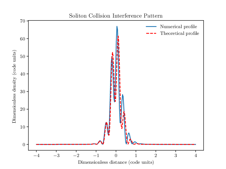
The outcomes of ULDM soliton collisions depend critically on whether the total energy of the isolated binary system is positive or negative. With a positive total energy the solitons pass through each other, emerging largely undisturbed from their initial configurations and the wavefunctions describing the solitons are superposed during the collision, yielding distinctive interference patterns.
Following [10], we consider the head-on collision of two solitions with mass ratio and high relative velocity. While we work in dimensionless code units, it should be noted that a dimensionful velocity can be restored from the code velocity by multiplying through by , the scale parameters defined in Equations 9 and 10. This simple case of a head-on soliton collision can be treated approximately. Starting from equation 31 we write the total wavefunction of the binary system in terms of dimensionless quantities along the collision axis as
| (35) |
where and are the initial central positions of the solitions, and are the soliton velocities, is a constant relative phase term and , parameterising the density profiles as discussed in Section 3.2. For convenience we set and . We expect that the interference effects will be maximised when two components of the wavefunction are centred at the same location, such that . This corresponds to a time , where in this simplified model we do not account for distortions caused by the accelerating or compactifying effects that the gravitational interaction has on the soliton profiles as they approach one another. The dimensionless density is then given by
| (36) |
Figure 1 shows the dimensionless density profile at the time of maximal interference for two solitons with mass ratio 2 and phase difference . The numerical result obtained using PyUltraLight closely matches the theoretical prediction of equation 36. Small disparities between the numerical and theoretical profiles may be attributed to the effect of gravitational contraction not included in the theoretical prediction of equation 36 and to a small offset in the true time of maximal interference due to the solitons accelerating as they fall together. We do not expect an exact match, but we have verified that PyUltraLight qualitatively reproduces the wave interference effects of the ULDM model. With the exception of [10], few studies of ULDM dynamics have investigated the interference patterns generated by colliding solitons in this way. In some cases, this is because the algorithm employed to simulate the dynamics is not capable of reproducing such effects. An example of this is given in [17], where it is demonstrated that the coarse-grained nature of the particle-mesh method renders the algorithm incapable of reproducing detailed interference patterns such as those shown here.
4.2 Effective Forces From Destructive Interference

As demonstrated in [26], the wavelike properties of ULDM give rise to effective forces which can dramatically affect the dynamics of core collisions. These effective forces arise as a result of interference phenomena, rather than because of any local interactions the ULDM model might incorporate. Figure 2 shows the results of a head-on collision between two solitons, where in one instance the solitons have no initial phase difference, and in the other instance a phase difference of is applied in the initial conditions. In this simulation, solitons of mass 20 are initialised with relative velocity 20 and initial separation 1.2 (code units). The solitons are allowed to collide, and contours of the density profile along the plane of symmetry are displayed. In one case (top) there is no phase offset between the initial solitons, while in the second the phases differ by . In the latter case, the phase shift creates an effective repulsive force between the two solitons. It can be seen in the second frame that as the solitons approach one another, the phase shift results in a slowing of the approach accompanied by a deformation of the density profile, acting so as to avoid contact between the solitons. Dissimilarly, in the case where there is no phase shift, the solitons readily collide and merge to form a single contiguous density profile prior to re-separating. Further discussion of this phenomenon and its possible observational consequences can be found in [26].
4.3 Tidal Disruption of Solitons Orbiting a Central Potential
PyUltraLight allows the inclusion of a static potential equivalent to a point-mass at the centre of the simulation region. There is no backreaction on this mass as a result of the ULDM dynamics, and its “mirror images” within the periodic coordinate systems are not accounted for within the overall gravitational potential. While a potential of this form does not necessarily accurately emulate that which we might expect from a realistic galaxy or dark matter halo, it provides a starting point for a study of the stability of satellite dark matter halos orbiting a much larger object. In particular, this includes the investigation of lifespans of dwarf satellite galaxies orbiting much larger objects (including the Milky Way) which are a key to understanding whether ULDM models can resolve the so-called missing satellites problem [44].
An extensive study of the tidal disruption of ULDM solitonic cores orbiting a central potential has recently been undertaken in [45] and we reproduce just one of their results here. To do this, we again adopt the definitions 32, namely
| (37) |
where we are working in dimensionless code units. Using these definitions, the Schrödinger-Poisson system can be recast in terms of hydrodynamical quantities in the so-called Madelung representation. The Madelung equations resemble the continuity and Euler equations of classical fluid dynamics, with the addition of a ‘quantum pressure’ term accounting for resistance against gravitational collapse. The Madelung formalism is discussed in detail in [43, 46, 47, 48]. Because this hydrodynamical formulation defines the fluid velocity as the gradient of the phase of the field , problems arise when , where the phase is not well defined. Because of this issue, the Madelung and Schrödinger representations are not strictly equivalent unless a quantisation condition is imposed, as discussed in [49]. We do not consider the subtleties of the Madelung representation here, as it is sufficient for our purposes to consider the fluid velocity in the region of a solitonic core, where no field nodes are present.33 3 It should be noted that, restoring dimensionful units, the fluid velocity is related to the ususal quantum mechanical probability current through For a discussion of the possible remedies to the ‘nodes problem’, the reader is referred to Chapter 15.3 of [50]. Where the Madelung representation is well defined, i.e. where the phase is a smoothly varying function, the velocity field of the Schrödinger-Poisson system is strictly irrotational, . If a radially symmetric soliton is initialised in a circular orbit around a Newtonian potential, there will be initial transient behaviour as the spherical profile becomes elongated along the radial direction of the central potential. Meanwhile, the velocity field corresponding to the overall orbital motion of the soliton will be superposed with the internal velocity field, combining so as to produce a net flow with vanishing curl.
The family of Riemann-S ellipsoids describe non-axisymmetric uniformly rotating bodies whose internal velocity fields have vanishing curl [51]. Therefore, it is the characteristic internal velocity field of a Riemann-S ellipsoid which we expect to arise during our simulation of a soliton orbiting a central mass. It is found in [45] that an initially spherical solitonic core without self-rotation will gradually spin up to form a tidally-locked ellipsoid with an irrotational internal velocity field when orbiting a host mass. We reproduce this result using PyUltraLight. Figure 3 shows the internal velocity field of a solitonic satellite after one complete revolution around a host mass. The soliton has become elongated along the radial line connecting it to the host, indicating that it is tidally locked, while the velocity field within the tidal radius is visibly irrotational and bears the qualitative trademarks of the Riemann-S ellipsoid as presented in Figure 2 of [52].
It should be noted that the wider velocity field is not expected to be accurately predicted in a simulation of this kind, though the field within the tidal radius is well-modelled. This is because the initial soliton density profile is defined only out to a given cutoff radius, beyond which the field value is set identically to zero. As mentioned previously, the Madelung hydrodynamical formulation of the Schrödinger-Poisson system is not valid where . Because of this, we focus primarily on the internal velocity field within the high density region of the solitonic core. As we have seen, in this region PyUltraLight is able to accurately reproduce the expected velocity field characteristics.
5 Convergence and Validation
5.1 Energy Conservation


Physically, we expect that the overall energy in the system will be conserved. This provides a test on the numerical performance of PyUltraLight, and we find that even at relatively low spatial resolution we see sub-percent level energy conservation for all the dynamical scenarios considered here. In this Section we express the energy of the Schrödinger-Poisson system in terms of the variables and and discuss its decomposition into individual constituents calculated separately within the code. We then present results for a variety of configurations.
We begin by defining a suitable action which yields the full Schrödinger-Poisson system through its corresponding Euler-Lagrange equations. We find that variation of
| (38) |
with respect to , and yields equations 14, 13, and the conjugate of equation 13, respectively. The integrand of equation 38 is the Lagrangian density, , from which we can derive the conserved energy in the usual way:
| (39) |
Evaluating this expression, we obtain:
| (40) | ||||
| (41) | ||||
| (42) |
where in the last step we have used Stokes’ Theorem as well as the Poisson equation (14) to perform simplifications. Because we are working with the dimensionless quantities defined in equation 12, it is easy to see that this quantity is related to the physical energy through multiplication by a constant factor of . It should be noted that equation 42 is not equivalent to the expectation value of the Schrödinger Hamiltonian, which is itself not a conserved quantity of the Schrödinger-Poisson system and is given by
| (43) |
The two terms in the integral 42 are calculated separately within the code. The first term is the gravitational potential energy of the Schrödinger-Poisson system, . As discussed in [5], the second term may be decomposed into contributions which may be considered separately as kinetic and ‘quantum’ energies, and . However, for our purposes it is sufficient to consider only their combined contribution. When PyUltraLight includes the central potential of a point mass located at the centre of the simulation grid we have additional energy contributions and calculate the gravitational potential energy from self-interactions separately from the gravitational potential energy due to the central potential.
Figures 4 and 5 demonstrate energy conservation for two scenarios. The first case shows the evolution of the energy of a single soliton undergoing significant tidal disruption within a Newtonian central potential. For this simulation a soliton of mass 12 in code units was initialised at a radial distance of 3 code units from the centre of a Newtonian central potential generated by a central mass of 1000 code units. As the soliton is disrupted, the kinetic energy increases, while the gravitational energy due to the central potential decreases, as expected. Meanwhile, the gravitational potential energy from self-interactions gradually increases toward zero as the disruption continues and the ULDM is halo spread over a greater area. In this case the sum of the individual energy components is conserved to at a resolution of .
Figure 5 demonstrates the evolution of the energy of a binary system of solitons in elliptical orbits around their common centre of mass over three orbital periods. In dimensionless code units, the soliton masses are 22, the initial separation 2, and the initial relative velocity was 3.6. At points of closest approach the kinetic energy increases as the solitons speed up, while the potential energy due to self-interaction decreases commensurately such that the total energy is conserved. In this scenario no central potential has been included. As the solitons reach the first point of closest approach, they become slightly deformed, exciting oscillatory modes which are manifest in the Figure as small scale oscillations superposed on the global behaviour. Figure 6 demonstrates the relationship between the total integrated energy and the grid resolution for the same binary system of solitons used to generate Figure 5. The vertical axis shows the ratio of the deviation in the total energy to the initial value of the energy, where the deviation is measured as the difference between the current and initial values. Energy is conserved at sub-percent level even at low resolutions (), and increasing grid resolution greatly improves accuracy.
Figure 7 demonstrates the improvement in energy conservation with increasing grid resolution for a single soliton tidally disrupted in a Newtonian central potential, with the same set up as used in Figure 4. Namely, a single soliton of mass 12 code units is initialised at a distance of 3 code units from a central mass, . The initial velocity of the soliton is where is the radial distance of the soliton from the central mass. The duration of the simulation is 0.5 code units so that the soliton undergoes significant tidal disruption as demonstrated in Figure 4. While we see that energy is conserved at sub-percent level even for grid resolution, the qualitative behaviour of the mass density distribution in this case is not correct, so we conclude that this resolution is insufficient for convergence despite good energy conservation. This highlights the importance of a multifaceted approach to convergence testing. At , energy is conserved to parts in .
5.2 Spatial and Temporal Resolution
We now examine the convergence of the field configuration as a function of spatial resolution and timestep in a typical simulation. We initialise PyUltraLight with two diametrically opposed solitons orbiting a large Newtonian central potential, running until the solitons are tidally disrupted, as shown in Figure 8.
To examine the sensitivity of the field configuration to the spatial resolution, we first run at with the default timestep. We then re-run at resolutions from to with the timestep fixed to the value and downsample the final outputs to . We sort the resulting values by the density at the corresponding spatial location, and plot differences in the phase and the magnitude of relative to the values of the run as shown in Figure 9 (bottom). The convergence is poor at , but improves with resolution, to the point that there is little difference between the and cases.
To examine the sensitivity of the the field configuration to the timestep, we take the same default simulation at , and then compare this to runs with timesteps 0.1, 10, and 50 times the default and down-sample the final output arrays to . We sort sort the array values in order of the field magnitude in the run with the smallest timestep and in Figure 10 we show the difference in the phase and magnitude of as a function of the timestep. The difference between the results with the default timestep and a value 10 times smaller are negligible; and there is reasonable agreement between the default case and those with the timestep boosted by a factor of 10. However, when the timestep is increased by a factor of the accuracy of both the phase and magnitude data are significantly reduced.
Figure 11 shows profiles of the density through the simulation volume, as a function of spatial resolution and timestep. Each plot represents the density profile down the axis of symmetry of the initial configuration (vertical axis in Figure 8) after approximately half a revolution around the central potential, or t=0.28 code units – slightly after the final frame in Figure 8 - when the solitons have become distorted due to tidal forces, but are not yet completely disrupted. We see that as the timestep is varied from 0.1 to 50 times the default value, the results with the default and the shorter timestep are virtually indistinguishable, and results are still reasonably accurate at 10 times the default timestep, with small deviations at high densities. However, the results are significantly distorted at 50 times the default timestep. We also see that as the spatial resolution is decreased from to , the lowest resolution performs poorly, but there is good convergence at resolutions of and above.


6 Discussion and Outlook
PyUltraLight is an accurate, flexible and easy to use tool for studying the dynamics of ultralight dark matter governed by the Schrödinger-Poisson system of equations. The code makes use of a pseudospectral symmetrised split-step Fourier methodology, in which all spatial derivatives are treated via explicit multiplication in the Fourier domain, thereby avoiding difficulties associated with finite-differencing methods.
Energy conservation within PyUltraLight is excellent, at sub-percent level for simulations run at , with even better performance as resolution is increased. The code captures complex phenomena resulting from the wave-like properties of ultralight dark matter, including the interference patterns arising during high-velocity collisions of solitonic cores, and effective forces observed in cases where the colliding cores are out of phase. These phenomena can be clearly observed at relatively low spatial resolution, avoiding the need for high-performance computing infrastructure to study the fundamental behaviour of ULDM systems in simple configurations. This makes PyUltraLight a useful tool for investigating the dynamics of ULDM systems.
PyUltraLight is Python-based, and as such is particularly simple to understand and use. The accompanying Jupyter notebook allows for the efficient adjustment of simulation parameters, and offers a useful browser interface for quick visualisation of simulation results. While Python-based, the code makes use of low-level language resources, namely the FFTW libraries through the use of the Pythonic pyFFTW wrapper and will operate at efficiency on a 16 core desktop workstation, suggesting that it is computationally efficient.
The current implementation of PyUltraLight is already a useful tool for simulating dynamical ULDM systems and exploring their dynamics However, there is much scope for improvement. In particular, future releases may incorporate a variable timestep and more sophisticated physics, including explicit self-interactions in the axion sector or additional matter components. Augmented versions of the code may also include higher-order generalisations of the pseudo-spectral method, such as those used in [53]. PyUltraLight is publicly available under a BSD license.
Acknowledgements.
We thank Xiaolong Du, Lam Hui, David Marsh, Nathan Musoke, Jens Niemeyer, and Chanda Prescod-Weinstein for valuable discussions on axion / ULDM cosmology, and thank Miro Erkintalo for advice on Schrödinger-Poisson solvers in optical systems. We acknowledge support from the Marsden Fund of the Royal Society of New Zealand, and the use of the New Zealand eScience Infrastructure (NeSI) high-performance computing facilities, which are funded jointly by NeSI’s collaborator institutions and through the Ministry of Business, Innovation & Employment’s Research Infrastructure programme https://www.nesi.org.nz.Appendix A Download and Licensing
PyUltraLight is publicly available under a BSD licence. The full repository, including supplementary files such as the code used to generate soliton profiles, is available on GitHub at https://github.com/auckland-cosmo/PyUltraLight. PyUltraLight makes use of the pyFFTW pythonic wrapper around the FFTW C-based fast Fourier transform libraries. Both pyFFTW and FFTW are freely-available and PyUltraLight has been used successfully on both Mac OS and Linux systems, as well as a shared-memory cluster environment. We welcome advice and feedback from users.
References
- (1) Planck Collaboration, P. A. R. Ade et al., Planck 2015 results. XIII. Cosmological parameters, Astron. Astrophys. 594 (2016) A13, [arXiv:1502.01589].
- (2) PandaX-II Collaboration, A. Tan et al., Dark Matter Results from First 98.7 Days of Data from the PandaX-II Experiment, Phys. Rev. Lett. 117 (2016), no. 12 121303, [arXiv:1607.07400].
- (3) LUX Collaboration, D. S. Akerib et al., Results from a search for dark matter in the complete LUX exposure, Phys. Rev. Lett. 118 (2017), no. 2 021303, [arXiv:1608.07648].
- (4) P. Bull et al., Beyond CDM: Problems, solutions, and the road ahead, Phys. Dark Univ. 12 (2016) 56–99, [arXiv:1512.05356].
- (5) L. Hui, J. P. Ostriker, S. Tremaine, and E. Witten, Ultralight scalars as cosmological dark matter, Phys. Rev. D95 (2017), no. 4 043541, [arXiv:1610.08297].
- (6) J. E. Kim and G. Carosi, Axions and the Strong CP Problem, Rev. Mod. Phys. 82 (2010) 557–602, [arXiv:0807.3125].
- (7) D. J. E. Marsh, Axion Cosmology, Phys. Rept. 643 (2016) 1–79, [arXiv:1510.07633].
- (8) W. Hu, R. Barkana, and A. Gruzinov, Cold and fuzzy dark matter, Phys. Rev. Lett. 85 (2000) 1158–1161, [astro-ph/0003365].
- (9) D. J. E. Marsh and A.-R. Pop, Axion dark matter, solitons and the cusp-core problem, Mon. Not. Roy. Astron. Soc. 451 (2015), no. 3 2479–2492, [arXiv:1502.03456].
- (10) B. Schwabe, J. C. Niemeyer, and J. F. Engels, Simulations of solitonic core mergers in ultralight axion dark matter cosmologies, Phys. Rev. D94 (2016), no. 4 043513, [arXiv:1606.05151].
- (11) E. Madelung, Eine anschauliche Deutung der Gleichung von Schrödinger, Naturwissenschaften 14 (Nov, 1926) 1004–1004.
- (12) J. Zhang, Y.-L. S. Tsai, J.-L. Kuo, K. Cheung, and M.-C. Chu, Ultralight Axion Dark Matter and Its Impact on Dark Halo Structure in -body Simulations, Astrophys. J. 853 (2018), no. 1 51, [arXiv:1611.00892].
- (13) V. Springel, The Cosmological simulation code GADGET-2, Mon. Not. Roy. Astron. Soc. 364 (2005) 1105–1134, [astro-ph/0505010].
- (14) “https://github.com/liambx/Axion-Gadget.”
- (15) M. Nori and M. Baldi, AX-GADGET: a new code for cosmological simulations of Fuzzy Dark Matter and Axion models, Mon. Not. Roy. Astron. Soc. 478 (2018) 3935, [arXiv:1801.08144].
- (16) P. Mocz and S. Succi, Numerical solution of the nonlinear Schrödinger equation using smoothed-particle hydrodynamics, Phys. Rev. E91 (2015), no. 5 053304, [arXiv:1503.03869].
- (17) J. Veltmaat and J. C. Niemeyer, Cosmological particle-in-cell simulations with ultralight axion dark matter, Phys. Rev. D94 (2016), no. 12 123523, [arXiv:1608.00802].
- (18) A. Almgren, J. Bell, M. Lijewski, Z. Lukic, and E. Van Andel, Nyx: A Massively Parallel AMR Code for Computational Cosmology, Astrophys. J. 765 (2013) 39, [arXiv:1301.4498].
- (19) A. J. Benson, Galacticus: A Semi-Analytic Model of Galaxy Formation, New Astron. 17 (2012) 175–197, [arXiv:1008.1786].
- (20) X. Du, C. Behrens, and J. C. Niemeyer, Substructure of fuzzy dark matter haloes, Mon. Not. Roy. Astron. Soc. 465 (2017), no. 1 941–951, [arXiv:1608.02575].
- (21) V. Springel, E pur si muove: Galiliean-invariant cosmological hydrodynamical simulations on a moving mesh, Mon. Not. Roy. Astron. Soc. 401 (2010) 791, [arXiv:0901.4107].
- (22) P. Mocz, M. Vogelsberger, V. H. Robles, et al., Galaxy formation with BECDM - I. Turbulence and relaxation of idealized haloes, Mon. Not. Roy. Astron. Soc. 471 (2017), no. 4 4559–4570, [arXiv:1705.05845].
- (23) H.-Y. Schive, Y.-C. Tsai, and T. Chiueh, GAMER: a GPU-Accelerated Adaptive Mesh Refinement Code for Astrophysics, Astrophys. J. Suppl. 186 (2010) 457–484, [arXiv:0907.3390].
- (24) “https://github.com/gamer-project/gamer/wiki.”
- (25) H.-Y. Schive, T. Chiueh, and T. Broadhurst, Cosmic Structure as the Quantum Interference of a Coherent Dark Wave, Nature Phys. 10 (2014) 496–499, [arXiv:1406.6586].
- (26) A. Paredes and H. Michinel, Interference of Dark Matter Solitons and Galactic Offsets, Phys. Dark Univ. 12 (2016) 50–55, [arXiv:1512.05121].
- (27) R. Easther, H. Finkel, and N. Roth, PSpectRe: A Pseudo-Spectral Code for (P)reheating, JCAP 1010 (2010) 025, [arXiv:1005.1921].
- (28) M. A. Amin, R. Easther, and H. Finkel, Inflaton Fragmentation and Oscillon Formation in Three Dimensions, JCAP 1012 (2010) 001, [arXiv:1009.2505].
- (29) M. A. Amin, R. Easther, H. Finkel, R. Flauger, and M. P. Hertzberg, Oscillons After Inflation, Phys. Rev. Lett. 108 (2012) 241302, [arXiv:1106.3335].
- (30) S.-Y. Zhou, E. J. Copeland, R. Easther, et al., Gravitational Waves from Oscillon Preheating, JHEP 10 (2013) 026, [arXiv:1304.6094].
- (31) “https://hgomersall.github.io/pyFFTW/.”
- (32) M. Frigo and S. G. Johnson, “http://www.fftw.org/.” "http://www.fftw.org/".
- (33) S. A. Q. Young, Signature Changing Spacetimes and WKB Approximations in General Relativity. Honors thesis, The University of Texas at Austin, 2015.
- (34) I. Dabo, B. Kozinsky, N. E. Singh-Miller, and N. Marzari, Electrostatics in periodic boundary conditions and real-space corrections, Phys. Rev. B 77 (Mar, 2008) 115139.
- (35) H.-Y. Schive, M.-H. Liao, T.-P. Woo, et al., Understanding the Core-Halo Relation of Quantum Wave Dark Matter from 3D Simulations, Phys. Rev. Lett. 113 (2014), no. 26 261302, [arXiv:1407.7762].
- (36) G. Agrawal, Nonlinear Fiber Optics. Optics and Photonics Series. Academic Press, 2013.
- (37) Q. Zhang and M. I. Hayee, Symmetrized Split-Step Fourier Scheme to Control Global Simulation Accuracy in Fiber-Optic Communication Systems, Journal of Lightwave Technology 26 (Jan, 2008) 302–316.
- (38) O. V. Sinkin, R. Holzlohner, J. Zweck, and C. R. Menyuk, Optimization of the split-step Fourier method in modeling optical-fiber communications systems, Journal of Lightwave Technology 21 (Jan, 2003) 61–68.
- (39) M. Frigo and S. G. Johnson, The Design and Implementation of FFTW3, Proceedings of the IEEE 93 (2005), no. 2 216–231. Special issue on “Program Generation, Optimization, and Platform Adaptation”.
- (40) “http://numexpr.readthedocs.io/.”
- (41) M. A. Ajaib, Numerical Methods and Causality in Physics, arXiv:1302.5601.
- (42) T. R. Taha and M. J. Ablowitz, Analytical and Numerical Aspects of Certain Nonlinear Evolution Equations. II. Numerical, Nonlinear Schrodinger Equation, J. Comput. Phys. 55 (1984) 203–230.
- (43) A. Suárez and T. Matos, Structure Formation with Scalar Field Dark Matter: The Fluid Approach, Mon. Not. Roy. Astron. Soc. 416 (2011) 87, [arXiv:1101.4039].
- (44) D. H. Weinberg, J. S. Bullock, F. Governato, R. Kuzio de Naray, and A. H. G. Peter, Cold dark matter: controversies on small scales, Proc. Nat. Acad. Sci. 112 (2015) 12249–12255, [arXiv:1306.0913].
- (45) X. Du, B. Schwabe, J. C. Niemeyer, and D. Bürger, Tidal disruption of fuzzy dark matter subhalo cores, Phys. Rev. D97 (2018), no. 6 063507, [arXiv:1801.04864].
- (46) A. Suárez and P.-H. Chavanis, Hydrodynamic representation of the Klein-Gordon-Einstein equations in the weak field limit, J. Phys. Conf. Ser. 654 (2015), no. 1 012008, [arXiv:1504.01164].
- (47) R. Johnston, A. N. Lasenby, and M. P. Hobson, Cosmological fluid dynamics in the Schrödinger formalism, arXiv:0904.0611.
- (48) M. Kopp, K. Vattis, and C. Skordis, Solving the Vlasov equation in two spatial dimensions with the Schrödinger method, Phys. Rev. D96 (2017), no. 12 123532, [arXiv:1711.00140].
- (49) T. C. Wallstrom, Inequivalence between the Schrodinger equation and the Madelung hydrodynamic equations, Phys. Rev. A49 (1994) 1613–1617.
- (50) R. E. Wyatt, Quantum Dynamics with Trajectories. Introduction to quantum hydrodynamics, vol. 28. 2005.
- (51) S. Chandrasekhar, The Equilibrum and the Stability of the Riemann Ellipsoids. I., Astrophys. J. 142 (Oct., 1965) 890.
- (52) T. Rindler-Daller and P. R. Shapiro, Angular Momentum and Vortex Formation in Bose-Einstein-Condensed Cold Dark Matter Haloes, Mon. Not. Roy. Astron. Soc. 422 (2012) 135–161, [arXiv:1106.1256].
- (53) D. G. Levkov, A. G. Panin, and I. I. Tkachev, Gravitational Bose-Einstein condensation in the kinetic regime, arXiv:1804.05857.