Binding Energy and Lifetime of Excitons in Metallic Nanotubes
Abstract
The difficulty of describing excitons in semiconducting single-wall nanotubes analytically lies with the fact that excitons can neither be considered strictly one- nor two-dimensional objects. However, the situation changes in the case of metallic nanotubes where, by virtue of screening from gapless metallic subbands, the radius of the exciton becomes much larger than the radius of the nanotube . Taking advantage of this, we develop the theory of excitons in metallic nanotubes, determining that their binding energy is about , in agreement with the existing experimental data. Additionally, because of the presence of the gapless subbands, there are processes where bound excitons are scattered into unbound electron-hole pairs belonging to the gapless subbands. Such processes lead to a finite exciton lifetime and the broadening of its spectral function. We calculate the corresponding decay rate of the excitons.
pacs
73.21.Hb, 73.22.-fI Introduction
An exciton is a bound state of an electron and a hole formed by their Coulomb attraction–the solid state analogy of a hydrogen atom, but with a larger size and a smaller binding energy. The smaller binding energy is due to the screening of the mutual Coulomb interaction by bound electrons of the medium, described by its dielectric constant. Excitons typically exist in insulators and weakly doped semiconductors. Metallic and strongly doped semiconducting materials disfavor formation of excitons. This is the result of two factors. First, as the conduction band is populated (e.g. by doping), screening by free charges strongly reduces the magnitude of the electron-hole Coulomb interaction and decreases its binding energy. Second, population of the conduction band reduces the number of quantum states available to accommodate the electron after its (virtual) scattering off the hole, further decreasing the binding energy, to the point where no meaningful bound state may be formed anymore.
This situation changes in quasi-one-dimensional systems, such as metallic nanotubes,[1] where formation of excitons occurs in subbands different from the subbands that are responsible for metallic screening. Such separation occurs as a result of quantization of the circumferential momentum. This makes exciton a well-defined excitation. Excitons in metallic single-walled carbon nanotubes (SWNTs) were experimentally observed in Refs. [2, 3]. Their binding energy was found to be about 50 meV, an order of magnitude smaller than the typical bandgaps of semiconducting nanotubes. Theoretically, excitons in metallic SWNTs were first studied by Ando under the effective-mass approximation.[4] Later, the binding energy of the exciton was addressed by first principles calculations[5, 6, 7] and also by the density matrix theory,[8] with the latter results being in agreement with experimental measurements. A brief review of excitonic effects in metallic SWNTs was given in Ref. [9]. However, to our knowledge, no simple analytical description of excitons in metallic nanotubes has been developed. It is the purpose of the present paper to fill this gap.
Let us illustrate the difficulty of describing excitons analytically in semiconducting SWNTs, stemming from the fact that excitons can neither be considered one-dimensional (1D) nor two-dimensional (2D) excitations. Indeed, consider the lowest energy subbands with the spectrum , and expand it near the bottom of the subband,
| (1) |
The bandgap is typically, , where is the radius of the nanotube. For convenience, we set throughout the paper. (In particular, in the zone-folding tight-binding approximation both the (8,0) and (10,0) zigzag nanotubes have ).
Because the electron-hole interaction energy is , the exciton binding energy can be estimated by minimizing,
| (2) |
taking into account the uncertainty relation, . This yields,
| (3) |
Since , we obtain that and, consequently, the exciton radius . Because to consider excitons to be 1D one would need to have , and conversely, to view them as 2D one would require , the semiconducting problem falls instead between the two limits where a numerical analysis is necessary. However, as we are going to see below, the situation changes in the case of metallic nanotubes where–by virtue of screening by the metallic subbands–the exciton binding energy decreases significantly (as already evidenced by the experimental data). As a result, the radius of the exciton increases, , and treatment of the exciton as a quasi-one-dimensional object becomes possible. This is what makes the analytic solution viable.
In this paper, we determine the binding energy and lifetime of an exciton in metallic SWNTs taking into account the screening effects within the random phase approximation (RPA). A problematic feature of the 1D Coulomb problem is the singularity in the potential energy, which is not integrable (unlike in the three-dimensional situation). This feature was first addressed by Loudon [10] and later further extensively studied by others.[11, 12, 13, 14, 15] Loudon introduced the truncated Coulomb interaction with a positive constant to ensure that Coulomb potential is regular at small distances . In our problem, the nanotube radius appears naturally and no other cutoff is needed. Using a variational ansatz with a Gaussian trial function, we show below that the binding energy is (the value of corresponds to an armchair metallic nanotube)
| (4) |
The dependence of the binding energy exhibits a good agreement with the results obtained in Ref. [8] with the density matrix theory, see Table I. In contrast, ab initio methods yield only rather crude estimates of the binding energy.[2, 5, 6] This is because computational limitations do not permit calculations for large nanotubes. In addition, the technique of photoluminescence (PL) spectroscopy cannot be applied to obtain binding energies of metallic nanotubes, which makes it challenging to determine the binding energy of excitons in metallic SWNTs. This is because the exciton is likely to undergo a nonradiative decay to the nearby linear subbands instead of electron-hole recombination process with a photon released. Nonetheless, the exciton binding energies experimentally observed[2, 3] have the same order of magnitude as predicted by our calculations.
| M-NTs | Binding energies (meV) | |||
| This paper | Density matrix | ab initio | Exper. | |
| (12,0) | 86 | (88) | [6] | – |
| (13,1) | 76 | 78[8] | – | [3] |
| (10,10) | 60 | (61) | [6] | – |
| (21,21) | 28 | (29) | – | [2 ] |
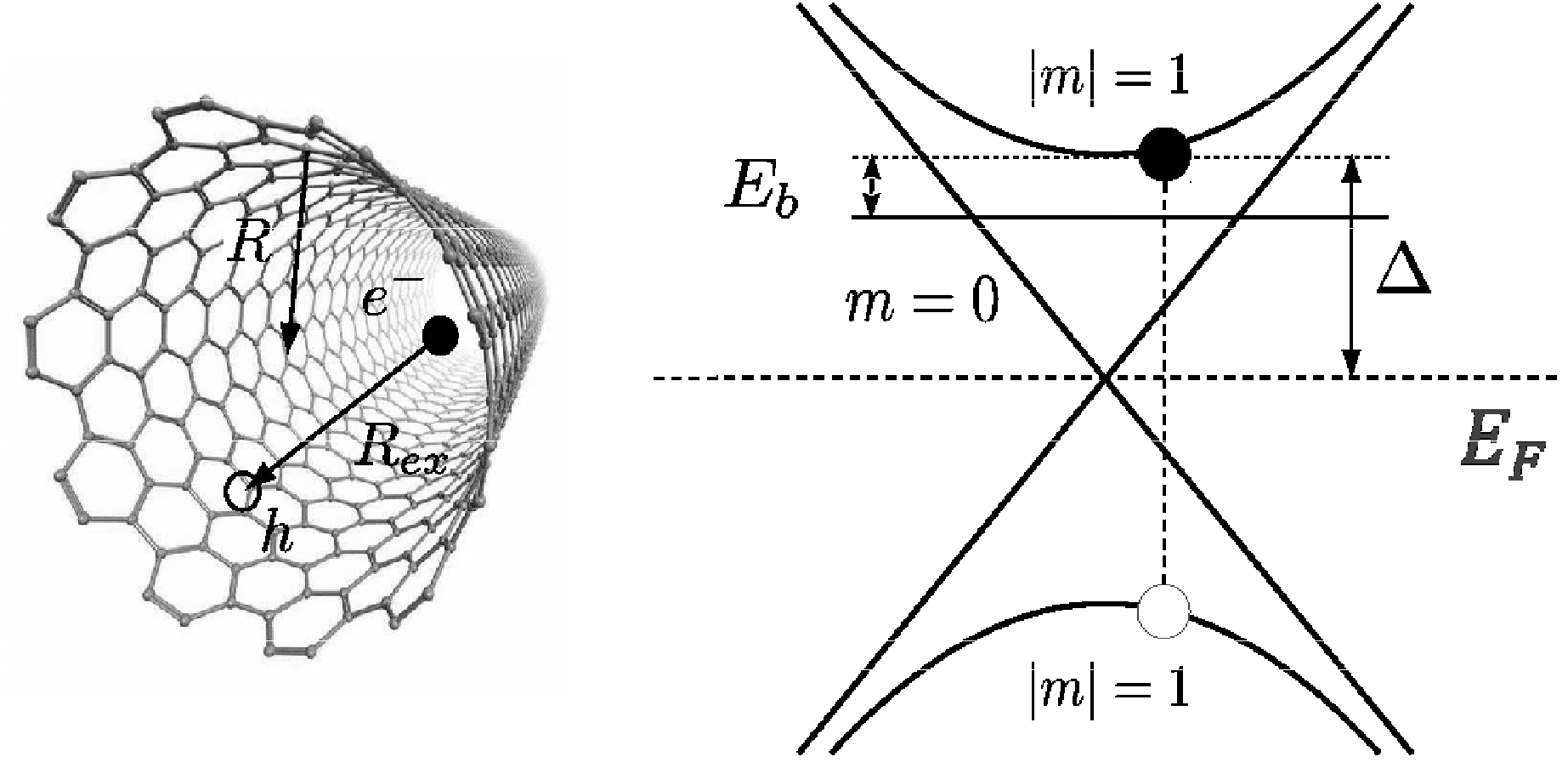
Furthermore, we explore the stability of excitons in metallic SWNTs, the question that is of fundamental interest but which remains unexplored in the existing theoretical works. The mechanism of a finite lifetime of the exciton can be illustrated by Fig. 1. The -th subband, corresponding to the integer angular quantum number , has the energy . Exciton bound states are formed between gapped, , subbands, and the lowest exciton is indicated by a dashed line in Fig. 1. This energy overlaps with the gapless subbands. Accordingly, an elastic transition of the electron and the hole from gapped to gapless subbands opens up a decay channel for the exciton.
To better understand the role of the Coulomb interaction in the formation and decay of the exciton, the following picture is helpful. The exciton is produced by multiple virtual scattering events of the electron and the hole within the gapped subbands. Such transitions are controlled by the Coulomb coupling , the subscript indicating that no angular momentum change takes place. These intrasubband transitions determine the binding energy of the exciton, see Fig. 2, left panel. The intersubband transitions–shown on the right panel in Fig. 2–appear as a result of the “dipolar” Coulomb interaction and occur with a change of the angular momentum of the electron (and with the opposite change of the angular momentum of the hole). We obtain that the ratio of the binding energy to the half-width of the exciton spectral function is
| (5) |
Such a ratio indicates that excitons in metallic SWNTs are well-defined excitations. This is consistent with experimental results obtained through ultrafast luminescence.[16] Below we derive our main results, Eqs. (4) and (5).
II The Hamiltonian of the system
The Coulomb interaction potential between two electrons located on the surface of a nanotube of radius at and is given by,
| (6) |
where and are the relative distance along the nanotube axis and the relative angle around the circumference of the nanotube. [In the case of an electron-hole pair, the sign of the interaction (6) is reversed.] If becomes large compared with a characteristic distance of the electron and the hole trajectories, the interaction approaches the Coulomb potential on a flat two-dimensional plane. On the other hand, if becomes small, Eq. (6) reduces to the “1D hydrogen” problem studied by Loudon. [10] The Coulomb interaction on the cylinder–the problem interpolating between and –was previously considered by Mahan[17] and Petersen.[18]
What is different in our case is the need to take into account screening, introduced by the gapless subbands of metallic SWNTs. This is most conveniently done by transitioning to the momentum space. The Fourier transform of the Coulomb interaction (6) yields the following expression,[4, 19]
| (7) | |||||
where is an integer number, and and are the modified Bessel functions of the first kind and second kind, respectively. However, because of the presence of conduction electrons in the gapless subbands, which move around in response to the “bare” Coulomb interaction , the actual (screened) interaction is modified: . This screened interaction disturbs the equilibrium of the system and induces density variations, which within the linear response are proportional to the strength of the interaction, , with the coefficient referred to as the polarization function (i.e. density-density correlation function) associated with the change in the angular momentum and the change in the linear momentum. The central tenet of RPA is the assumption of the mean field, which predicts that the variation of the density induces the additional potential in the system: . This additional potential together with the bare potential constitutes the total interaction: . This gives,
| (8) |
The formation of the exciton is mostly facilitated by the strongest interaction , which at low becomes logarithmically strong, . In contrast, the higher interaction harmonics, , remain constant in this limit, .

The screening of the interaction is determined by the uniform harmonics of the polarization function with no change in the angular momentum, given by,
| (9) |
where accounts for two spin directions and the presence of the two Dirac points within the Brillouin zone (see Appendix for details).
A large spatial radius of the exciton makes it sufficient to consider only the static limit of Eq. (9), where is disregarded compared with . Indeed, frequencies involved are of the order of the exciton binding energy, , where the effective mass , according to Eq. (1). On the other hand, the involved momenta are . Accordingly, the ratio . The screened Coulomb interaction in this static limit assumes the form,
| (10) |
where we introduced the dimensionless interaction strength where is taken to be the same as the velocity of electrons propagating in graphene, m/s.
To similarly calculate the screening of the interaction, one needs to know the polarization function associated with the change of the angular momentum. While the intrasubband value of at low and , as seen from Eq. (9), depends on which one of the two quantities tends to zero faster than the other, there is no such ambiguity for the intersubband polarization function : as shown in Appendix, . This gives for the screened intersubband interaction,
| (11) |
In the limit of large wavelengths, , the two interactions approach each other, . It should be pointed out, however, that while the interaction remains almost constant for finite but small , the interaction is rather sensitive to , with the derivative diverging at .
Note that in the absence of spectrum curvature, the polarization function of one-dimensional subbands is independent of temperature. It is also unmodified by the electron-electron interactions.[20] On the other hand, the polarization constant , which involves gapped subbands, has a negligible temperature dependence. Indeed, the population of thermally excited electron-hole pairs is , where is much larger than the thermal energy at room temperature. For these reasons it is sufficient to consider the screening of the Coulomb interaction at zero temperature. Similarly, small levels of doping, , do not affect the strength of the Coulomb interaction.
Having determined the magnitude of the electron-electron (and, therefore, electron-hole) interaction, we can proceed to calculate the energy and the lifetime of the exciton. The Hamiltonian of the system has the following form:
| (12) |
Here and are the operators for the particles residing on the upper and lower subbands with (or ); the operators and correspond to right and left moving particles of massless () subbands; the interaction describes scattering within the massive subbands whereas coupling describes processes where scattering occurs between massive and massless subbands. Note that of all of the Coulomb interaction terms we have retained only those that are responsible for the formation of the excition with zero total momentum: for example, the -term describes scattering of the electron with momentum () and the hole with momentum () into a pair of new states with momenta and .
The intersubband terms in the Hamiltonian (12) have the extra prefactor compared with the intrasubband transitions. The origin of this difference lies in the pseudospin nature of the underlying Hamiltonian of the two-dimensional graphene crystal that forms the nanotube. (The pseudospin arises from the existence of two atomic sublattices in the graphene honeycomb arrangement of carbon atoms.) As a result, two states of the same energy and opposite momenta are orthogonal to each other. More generally, the amplitude of the transition between the states having momenta and and the same sign of energy is suppressed by the factor , where is the angle that the momentum makes with the -axis. When graphene is rolled into a nanotube, the circumferential momenta are quantized, . The gapless states are those that move along the -axis: with or . In contrast, in the gapped subbands, , with the relevant momenta are near the bottom/top of the subbands: . Accordingly, the relevant states are those that have . Correspondingly, each particle transitioning between a gapless state and a gapped state (close to the bottom of the subband) introduces a factor into the amplitude of the scattering. For the two-particle Coulomb interaction , the total additional coefficient is, therefore, .
III Binding energy and lifetime
The wave function of the exciton is sought in the form
| (13) |
where is the ground state of the system where all individual electron states with the positive energy are empty and all states with the negative energy are occupied. The function describes the amplitude of the electron-hole pair to be in the gapped states whereas the function describes the likelihood of the pair to reside in the massless states. Note that in the last two terms we have explicitly taken into account that in the ground state the left-moving states are occupied as long as is positive whereas the right-moving states are occupied if is negative. Because the system is symmetric with respect to the symmetry between left- and right-moving states, the function must be symmetric: .
The Schrödinger equation separates into two coupled equations for the functions and :
| (14) |
Excluding from these equations and replacing the sums by the integrals, , we arrive at the following integral equation for the function ,
| (15) |
The singularities at lead to the imaginary part in the energy of the exciton. Because the resulting imaginary part is small compared with the bandgap, , it is sufficient to keep the infinitesimal in the denominator and utilize the Sokhotski identity, , for the calculation of the integral’s imaginary part. In contrast, the real part, which arises from the principal value of the integral, can be ignored. Although the real part appears to diverge logarithmically, such divergence is the artefact of our assumption that is constant. This approximation, in any case, fails for transferred momenta of the order , which should, therefore, be used as the upper cut-off for the logarithmic integral. Finally, because the energy involved is large, (rather than the small binding energy ), the logarithm is of the order and the real part of the last term in the brackets in Eq. (15) merely adds a contribution . This second-order correction is small compared to the main contribution from the term and may be ignored. Hence, we obtain from Eq. (15),
| (16) |
Below, the binding energy and the lifetime of the exciton,
| (17) |
are determined from the ground-state eigenvalue of this equation.
III.1 The shallow potential approximation
The fastest way to estimate the exciton binding energy is by utilizing the well-known in quantum mechanics shallow well approximation which in the momentum space amounts to replacing the interaction with its zero-momentum value . Equation (16) then becomes exactly solvable and yields,
| (18) |
The effective mass, cf. Eq. (1), can now be expressed via the bandgap, and the interaction constants and , given by Eqs. (10) and (11). This gives,
| (19) |
It is clear, however, that the value that follows from Eq. (19), significantly overestimates the binding energy of the exciton: as evidenced by Eq. (10), the function is irregular at where it has an infinite derivative. For this reason, the integrand in Eq. (16) in fact contributes much less to the integral where departs from than predicted by the shallow potential approximation. To make a better approximation, we are now going to utilize the variational approach.
III.2 The variational solution
To apply the variational approach to Eq. (16) we choose the Gaussian trial function,
| (20) |
or, equivalently, in the momentum space, . According to Eq. (16), the ground state energy of the exciton is the sum of the kinetic energy,
| (21) |
and the expectation value of the potential energy. The latter is a complex quantity: . The imaginary part determines the exciton lifetime,
| (22) |
while the real part yields, with the help of the momentum representation, the following integral:
| (23) |
The binding energy should be found by minimizing the sum with respect to . The integral in cannot be calculated exactly, but can be approximated rather accurately. First, it is convenient to utilize the dimensionless variables and to recast the average potential energy (10) in the form:
| (24) |
Next, we anticipate that for the large-radius excitons the small values of (and hence the small values of ) are relevant (This expectation that is supported by the final result). The function , whereas the Macdonald function has a logarithmic singularity, , where is the Euler constant. Finally, we notice that the logarithm depends on its argument rather weakly, in comparison with the exponential , and hence can be approximated as a constant within the relevant range of the -integration,
| (25) |
with some fitting parameter . Numerical calculation demonstrates that the value provides an excellent fit between the exact numerical integration of the left-hand side of Eq. (25) and its right-hand side for the value stated in Eq. (10), which corresponds to gapless modes.
Accordingly, we arrive at the following value of the binding energy, ,
| (26) |
where in the last line we used the definition of the coupling constant from Eq. (10) and also replaced the effective mass in terms of the bandgap .
The binding energy (26) has a maximum at , where the value stated in Eq. (4) is reached. This binding energy agrees well with the experimental measurements [2]. In turn, the obtained result justifies the approximations of a large exciton radius. Indeed, according to the wave function (20), the radius of the exciton is .
The exciton radius increases when the Coulomb interaction is further reduced if the nanotube is located on the surface of a dielectric substrate. Correspondingly, the dimensionless interaction strength will be modified as, , where is the dielectric constant of the substrate. The binding energy can still be calculated using Eq. (26). Table II shows the calculated binding energies for several substrates.
The decay of the exciton into the linear subbands was first studied numerically in Ref. [7] which concluded that such decay processes lead to a negligible broadening. Our result indicate otherwise and are also in a good agreement with experiments reported in Ref. [16].
| Substrates | Dielectric constant | Binding energy (meV) |
|---|---|---|
| 2.5 | 22.4 | |
| SiC | 3.75 | 18.7 |
| 4.4 | 17.9 | |
| GaAs | 7 | 13.8 |
The value of the inverse lifetime now follows from Eq. (22):
| (27) |
whose numerical value yields Eq. (5). The exciton acquires a significant broadening, but nonetheless remains a well-defined excitation. Interestingly, this ratio is numerically very close to the value predicted by the shallow potential approximation.
IV Summary and conclusions
Because of the presence of the gapless subbands, excitons in metallic carbon nanotubes acquire unique features that distinguish them from excitons in other solid state systems. First, the quasi-one-dimensional nature of nanotubes makes screening by conduction electrons less effective than in conventional metals. As a result, the electron-hole interaction remains significant enough to ensure the formation of a bound pair. Second, the separation (in the momentum space) of gapless states () from the subbands where the exciton is formed () and the fact that the latter subbands are fully gapped allow the electron and the hole to explore fully the gapped subbands, unlike what happens in a conventional doped semiconductor where filling of the conduction band quickly depletes the number of available electron states. Third, the screening by the gapless states is nonetheless significant enough so that the radius of the exciton is greater than the nanotube radius with the binding energy of the order of . This allows one to treat excitons as quasi-one-dimensional objects, unlike excitons in semiconducting nanotubes which are neither one-dimensional nor two-dimensional objects. Fourth, the presence of the gapless subbands opens up a channel for exciton attenuation where the electron and hole can scatter off each other into the gapless states. The presence of this channel leads to a considerable broadening of the exciton but not so significant as to smear it away completely.
This work was supported by the DOE, Office of Basic Energy Sciences, through Grant No. DE-FG02-06ER46313.
Appendix A Polarization function of a metallic nanotube
The screening of Coulomb interaction in a nanotube is determined by its polarization function which in the zone-folding approximation can be obtained from the polarization function of the underlying two-dimensional graphene crystal. The low-energy excitations in graphene are described by the Dirac Hamiltonian, , where is the Pauli matrix acting in the pseudospin space of the two triangular sublattices of carbon atoms. The polarization function,
| (28) |
relates to the product of two Green’s function of -electrons consisting of the contributions from both the upper cone () and lower cone (),
| (29) |
where is the projection of the pseudospin Pauli matrix onto the direction of electron momentum. At zero temperature the terms contribute,
| (30) |
The retarded counterpart of the polarization operator can be obtained through analytical continuation . However, since virtual transitions avoid all singular poles, a small imaginary constant can be disregarded for our purposes,
| (31) |
Within the zone folding approximation, which ignores any curvature effects on the electronic spectrum arising from the rolling of the graphene sheet, the polarization function for a nanotube is obtained by quantizing the circumferential momenta, , , and replacing the integral with the sum, . Additionally, to relate the resulting polarization function to the one-dimensional density, the quantity (31) should be multiplied by the factor . Expressing the cosine function in terms of the momentum component, we obtain:
| (32) | |||||
Of interest to us here are the polarization function for and . For and , only the terms should be retained. For example, for , the integral only extends over the interval (where the integrand does not depend on ) and the expression (9) is recovered, the subscript in being omitted. (The same result follows for .)
For , because only the static and homogeneous limit is important for our purposes, one can set and in Eq. (32). The remaining -integral is independent of and can be (together with the summation over ) calculated numerically. This yields
| (33) |
which yields the value of the screened interaction as in Eq. (11).
Note that the dominant contribution into the polarization function (33) comes from the lowest-order virtual transitions, and . Retaining only these contributions, one would obtain the estimate . Another good order-of-magnitude estimate could be obtained from the polarization function for graphene, . In the static limit, , replacing , and multiplying the result by , as explained above, one would obtain, , which overestimates the exact value (33) by only .
References
- [1] R. Saito, G. Dresselhaus, and M. S. Dresselhaus, Physical Properties of Carbon Nanotubes (Imperial College Press, London, 1998).
- [2] F. Wang, D. J. Cho, B. Kessler, J. Deslippe, P. J. Schuck, S. G. Louie, A. Zettl, T. F. Heinz, and Y. R. Shen, Phys. Rev. Lett. 99, 227401 (2007).
- [3] P. May, H. Telg, G. Zhong, J. Robertson, C. Thomsen, and J. Maultzsch, Phys. Rev. B 82, 195412 (2010).
- [4] T. Ando, J. Phys. Soc. Jpn. 66, 1066 (1997).
- [5] C. D. Spataru, S. Ismail-Beigi, L. X. Benedict, and S. G. Louie, Phys. Rev. Lett. 92, 077402 (2004).
- [6] J. Deslippe, C. D. Spataru, D. Prendergast, and S. G. Louie, Nano Lett. 7, 1626 (2007).
- [7] S. Uryu and T. Ando, Phys. Rev. B 77, 205407 (2008).
- [8] E. Malic, J. Maultzsch, S. Reich, and A. Knorr, Phys. Rev. B 82, 035433 (2010).
- [9] T. Ando and S. Uryu, Phys. Status Solidi C 6, 173 (2009).
- [10] R. Loudon, Am. J. Phys. 27, 649 (1959).
- [11] M. Andrew. Am. J. Phys. 34, 1194, (1966).
- [12] L. K. Haines, and D. H. Roberts, Am. J. Phys. 37, 1145, (1969).
- [13] M. Andrew, Am. J. Phys. 44, 1064, (1976).
- [14] J. F. Gomes, and A. H. Zimerman, Am. J. Phys. 48, 579, (1980).
- [15] R. E. Moss, Am. J. Phys. 55, 397, (1987).
- [16] T. Koyama, S. Shimizu, T. Saito, Y. Miyata, H. Shinohara, and A. Nakamura, Phys. Rev. B 85, 045428 (2012).
- [17] M. K. Kostov, M. W. Cole, and G. D. Mahan, Phys. Rev. B 66, 075407 (2002).
- [18] T. G. Pedersen, Phys. Rev. B 67, 073401 (2003).
- [19] E. G. Mishchenko, A.V. Andreev, and L. I. Glazman, Phys. Rev. Lett. 87, 246801 (2001).
- [20] I. E. Dzyaloshinskii and A. I. Larkin, Sov. Phys. JETP 38, 202 (1974).