The general scalar potential of the model defined above is given by:

$\displaystyle\begin{split}V(\Phi,\phi_{R})=&-\mu^{2}_{1}\,\mathrm{Tr}\left(\Phi^{\dagger}\Phi\right)+{\rm Re}\left[\mu_{12}^{2}\mathrm{Tr}\left(\Phi^{\dagger}\Phi^{c}\right)\right]-\mu^{2}_{R}\mathrm{Tr}\left(\phi_{R}^{\dagger}\phi_{R}\right)\\ &+\lambda_{1}\,\mathrm{Tr}^{2}\left(\Phi^{\dagger}\Phi\right)+\rm{Re}\left[\lambda_{2}\mathrm{Tr}^{2}\left(\Phi^{\dagger}\Phi^{c}\right)\right]+\rm{Re}\left[\lambda_{3}\mathrm{Tr}\left(\Phi^{\dagger}\Phi\right)\mathrm{Tr}\left(\Phi^{\dagger}\Phi^{c}\right)\right]\\ &+\left(\lambda_{4}-2\rm{Re}\lambda_{2}\right)\left|\mathrm{Tr}\left(\Phi^{\dagger}\Phi^{c}\right)\right|^{2}\\ &+\lambda_{R1}\mathrm{Tr}^{2}\left(\phi_{R}^{\dagger}\phi_{R}\right)+\lambda_{R2}\,\mathrm{Tr}\left(\phi_{R}^{\dagger}\phi_{R}\phi_{R}^{\dagger}\phi_{R}\right)\\ &+\lambda_{R\Phi 1}\mathrm{Tr}\left(\phi_{R}^{\dagger}\phi_{R}\right)\mathrm{Tr}\left(\Phi^{\dagger}\Phi\right)\,+\,\rm{Re}\left[\lambda_{R\Phi_{2}}\mathrm{Tr}\left(\phi_{R}\phi_{R}^{\dagger}\right)\mathrm{Tr}\left(\Phi^{\dagger}\Phi^{c}\right)\right]\\ &+\lambda_{R\Phi 3}\mathrm{Tr}\left(\phi_{R}^{\dagger}\phi_{R}\Phi^{\dagger}\Phi\right)\,.\end{split}$

(14)

The quartic couplings $\lambda_{2,3}$ and $\lambda_{R\Phi 2}$, and the dimensional term $\mu_{12}$, carry a non-trivial phase in case CP symmetry is explicitly broken. We have also introduced the conjugate field $\Phi^{c}\equiv\tau_{2}\Phi^{*}\tau_{2}$, $\tau_{2}$ being the standard Pauli matrix.

The most general Yukawa Lagrangian for the matter fields $\psi_{L/R}$ is ¹¹ 1 We consider for simplicity only Yukawa couplings to the third fermion generation and we omit the flavor index $i$ in $\psi_{L/R}$, see Eq. (6).

$\displaystyle\mathcal{L}_{\rm Yuk}^{\psi}$

$\displaystyle=$

$\displaystyle y\,\text{Tr}\left[\overline{\psi_{L}}\,\Phi\,\psi_{R}\right]\,+\,y_{c}\,\text{Tr}\left[\overline{\psi_{L}}\,\Phi^{c}\,\psi_{R}\right]\,+\,\text{h.c.}\,.$

(15)

In terms of the SM fermion fields Eq. (15) reads:

$\displaystyle\begin{split}\mathcal{L}_{\rm Yuk}^{\psi}\;=\;&y\left(\overline{t_{L}}\,t_{R}\,\phi_{1}^{0}+\overline{t_{L}}\,b_{R}\,\phi_{2}^{+}+\overline{b_{L}}\,t_{R}\,\phi_{1}^{-}+\overline{b_{L}}\,b_{R}\,\phi_{2}^{0}\right.\\ &\quad+\left.\overline{\nu_{L}}\,\nu_{R}\,\phi_{1}^{0}+\overline{\nu_{L}}\,\tau_{R}\,\phi_{2}^{+}+\overline{\tau_{L}}\,\nu_{R}\,\phi_{1}^{-}+\overline{\tau_{L}}\,\tau_{R}\,\phi_{2}^{0}\right)\\ &+y_{c}\left(\overline{t_{L}}\,t_{R}\,\phi_{2}^{0*}-\overline{t_{L}}\,b_{R}\,\phi_{1}^{+}-\overline{b_{L}}\,t_{R}\,\phi_{2}^{-}+\overline{b_{L}}\,b_{R}\,\phi_{1}^{0*}\right.\\ &+\left.\overline{\nu_{L}}\,\nu_{R}\,\phi_{2}^{0*}-\overline{\nu_{L}}\,\tau_{R}\,\phi_{1}^{+}-\overline{\tau_{L}}\,\nu_{R}\,\phi_{2}^{-}+\overline{\tau_{L}}\,\tau_{R}\,\phi_{1}^{0*}\right)\,\;+\;{\rm h.c.}\end{split}$

(16)

Electroweak symmetry breaking is induced by a nonzero vev of $\Phi$, which takes the form:

$$\langle\Phi\rangle\;=\;\left(\begin{array}[]{cc}u_{1}&0\\ 0&u_{2}\end{array}\right)\,,$$

(17)

with generally $u_{1}\neq u_{2}$. From Eq. (16) we have the fermion mass spectrum:

$\displaystyle\begin{split}m_{t}=m_{\nu_{\tau}}=(y\sin\beta+y_{c}\cos\beta)v\,,\\ m_{b}=m_{\tau}=(y\cos\beta+y_{c}\sin\beta)v\,,\end{split}$

(18)

where $v\equiv\sqrt{u_{1}^{2}+u_{2}^{2}}=174$ GeV and $\tan\beta\equiv u_{1}/u_{2}$. In the case of a self-conjugate bi-doublet field $\Phi\equiv\Phi^{c}$, one has $u_{1}=u_{2}$ in Eq. (17) and equality between fermion masses is enforced at tree-level, namely

$$m_{t}=m_{b}=m_{\tau}=m_{\nu_{\tau}}\,.$$

(19)

In order to separate the neutrino and top masses in Eq. (18) and Eq. (19) we implement the seesaw mechanism [41, 42, 43, 44] by adding a new chiral fermion singlet $N_{L}\sim(1,1,1)$, which has Yukawa interaction

$$\mathcal{L}_{\rm Yuk}^{N}\;=\;-y_{\nu}\,\overline{N_{L}}{\rm Tr}\left[\phi_{R}^{\dagger}\,\psi_{R}\right]\,+\,{\rm h.c.}$$

(20)

The latter generates a Dirac mass term $M_{R}\overline{N_{L}}\nu_{R}$, with $M_{R}\equiv y_{\nu}v_{R}$. The resulting Majorana mass term for the neutral fermion fields reads:

$\displaystyle\mathcal{L}_{\rm mass}^{\nu}\;=\;-\frac{1}{2}\left(\begin{array}[]{ccc}\overline{\nu_{R}^{c}}&\overline{\nu_{R}}&\overline{N_{R}^{c}}\end{array}\right)\left(\begin{array}[]{ccc}0&m_{t}&0\\ m_{t}&0&M_{R}\\ 0&M_{R}&0\end{array}\right)\left(\begin{array}[]{c}\nu_{L}\\ \nu_{L}^{c}\\ N_{L}\end{array}\right)\,+\,{\rm h.c.}$

with $\nu^{c}_{L/R}\equiv C\overline{\nu}_{R/L}^{T}$ and $N^{c}_{R}\equiv C\overline{N_{L}}^{T}$. The mass spectrum consists of one massless neutrino

$$\nu_{\tau L}=-\cos\theta\nu_{L}+\sin\theta N_{L}\,,$$

(29)

with $\tan\theta=m_{t}/M_{R}$, and one Dirac neutrino $N_{D}$ with mass $m_{D}=\sqrt{m_{t}^{2}+M_{R}^{2}}$ and chiral components:

$\displaystyle\begin{split}P_{L}\,N_{D}\;=\;&\nu_{L}\sin\theta+N_{L}\cos\theta\,,\\ P_{R}\,N_{D}\;=\;&\nu_{R}\,.\end{split}$

(30)

By adding a Majorana mass term for the singlet fermion $N_{L}$

$$\mathcal{L}_{\rm mass}^{N}=-\frac{1}{2}M_{N}\overline{N^{c}_{R}}\,N_{L}\,+\,{\rm h.c.}$$

(31)

the total lepton number is explicitly broken and the spectrum consists of three massive neutrinos. Taking $M_{N}\ll m_{t},M_{R}$, the mass eigenstates result in one light active Majorana neutrino $\nu_{\tau}$ with mass

$$m_{\nu_{\tau}}=M_{N}\frac{m_{t}^{2}}{m_{D}^{2}}$$

(32)

and two quasi-degenerate heavy Majorana neutrinos $N_{1,2}$ with opposite CP parities and masses

$$M_{1,2}=m_{D}\pm\frac{M_{N}}{2}\frac{M_{R}^{2}}{m_{D}^{2}}\,.$$

(33)

Threshold corrections may induce a sizable mass splitting between $m_{\tau}$ and $m_{b}$ in Eq. (18) and Eq. (19), which depends on the $G_{\rm PS}$ breaking scale $v_{R}$, see Ref. [45].

In the simplest scenario where the field $\Phi$ is self-conjugate, the fermion spectrum is degenerate, see Eq. (19), and the scalar potential in Eq. (14) consists of the quartic couplings $\lambda_{1}$, $\lambda_{R1,2}$ and $\lambda_{R\Phi 1,3}$. As discussed above, by adding a new chiral fermion $N_{L}$, which is a singlet under $G_{\rm PS}$, it is possible to induce a hierarchy between the top quark and neutrino masses via the seesaw mechanism, such that the correct light neutrino mass scale can be accommodated. Here, we further extend the matter content of the theory with a new vector-like fermion $F\sim(10,1,1)$ with mass $M_{F}$ and Yukawa interactions:

$\displaystyle\mathcal{L}_{\rm Yuk}^{F}$

$\displaystyle=$

$\displaystyle y_{F}\,{\rm Tr}\left(\overline{F_{L}}\,\phi_{R}^{T}\,i\tau_{2}\,\psi_{R}\right)\,+\,{\rm h.c.}$

(34)

In terms of the $SU(3)_{C}$ representations, the field $F$ can be decomposed as

$$F\;=\;\left(\begin{array}[]{cc}S&B\sqrt{2}\\ B^{T}\sqrt{2}&E\end{array}\right)\,,$$

(35)

where $S$, $B$ and $E$ denote a color sextet, triplet and singlet, respectively. Then, from Eq. (34) the fields $B$ and $E$ mix with the right-handed components of $\psi_{R}$, $b_{R}$ and $\tau_{R}$, respectively, giving the overall Dirac mass terms:

	$\displaystyle\mathcal{L}_{\rm mass}^{b}$	$\displaystyle=$	$\displaystyle\left(\begin{array}[]{cc}\overline{b_{L}}&\overline{B_{L}}\end{array}\right)\left(\begin{array}[]{cc}m_{t}&0\\ m_{B}&M_{F}\end{array}\right)\left(\begin{array}[]{c}b_{R}\\ B_{R}\end{array}\right)\,+\,{\rm h.c.}\,,$
	$\displaystyle\mathcal{L}_{\rm mass}^{\tau}$	$\displaystyle=$	$\displaystyle\left(\begin{array}[]{cc}\overline{\tau_{L}}&\overline{E_{L}}\end{array}\right)\left(\begin{array}[]{cc}m_{t}&0\\ \sqrt{2}\,m_{B}&M_{F}\end{array}\right)\left(\begin{array}[]{c}\tau_{R}\\ E_{R}\end{array}\right)\,+\,{\rm h.c.}\,,$

with $m_{B}\equiv y_{F}\,v_{R}/\sqrt{2}$. As a result of this mixing, the top quark becomes naturally heavier than the other SM fermions. In fact, in the limit $m_{B}\gg m_{t},\,M_{F}$, the $b$ quark and $\tau$ charged lepton masses satisfy the tree-level relation:

$$m_{b}\;=\;\sqrt{2}\,m_{\tau}\;\approx\;\frac{M_{F}\,m_{t}}{\sqrt{2}\,m_{B}}\,.$$

(48)

Analogously, we have a new vector-like quark, $\hat{B}$, and a new vector-like lepton, $\hat{E}$, with corresponding masses $M_{B}$ and $M_{E}$, which satisfy the tree-level relation:

$$M_{B}\;=\;M_{E}/\sqrt{2}\;\approx\;m_{B}\,.$$

(49)

In order to ensure asymptotic safety in the UV for all the system in Tab. 1, we employ the $1/N_{F}$ expansion approach developed in [15, 16, 17, 46], first applied to the whole SM in [31]. More specifically, we introduce $N_{F}\gg 1$ vector-like fermions, which transform non-trivially under $G_{\rm PS}$. In this framework, the RG equations receive a contribution at leading order in the $1/N_{F}$ expansion of the relevant Feynman diagrams, which are resumed as shown in Fig 1 (only gauge coupling cases are shown). This non-perturbative effect induces an interacting fixed point for both the Abelian and non-Abelian gauge interactions of the SM [31]. The fixed point is guaranteed by the pole structure occurred in the expressions of the summation [16, 17].

In the present scenario, we consider three sets of vector-like fermions charged under $G_{\rm PS}$, with the following charge assignment:

$$N_{F_{4}}\left(4,1,1\right)\oplus N_{F_{2L}}\left(1,3,1\right)\oplus N_{F_{2R}}\left(1,1,2\right)\,,$$

(50)

where the $N_{F_{2L}}$ vector-like fermions are chosen in the adjoint representation of $SU(2)_{L}$ to avoid fractional electrical charges. We have also chosen each set of vector-like fermions to have non-trivial charges only under one simple gauge group to avoid the extra contributions in the summation of semi-simple group.

To the leading $1/N_{F}$ order for each set, the higher order (ho) contributions (i.e. the bubble diagrams in Fig. 1) to the RG functions of the gauge couplings are calculated in [17], while for the abelian case they were first computed in [15]. Here we list a short summary of the results. The higher order contributions are give by:

$$\beta^{{\rm ho}}_{i}=\frac{2A_{i}\alpha_{i}}{3}\frac{H_{1_{i}}(A_{i})}{N_{F_{i}}},\hskip 11.49994pt\alpha_{i}\equiv\frac{g_{i}^{2}}{\left(4\pi\right)^{2}}~~\left(i=2L,\,2R,\,4\right)\,,$$

(51)

with the functions $H_{1i}$ and the t’Hooft couplings $A_{i}$ given by

$$\begin{split}A_{i}&=4\alpha_{i}T_{R}N_{F_{i}}\\ H_{1_{i}}&=\frac{-11}{2}N_{ci}+\int_{0}^{A_{i}/3}I_{1}(x)I_{2}(x)dx\hskip 22.99988pt\left(N_{ci}=2,4\right)\\ I_{1}(x)&=\frac{\left(1+x\right)\left(2x-1\right)^{2}\left(2x-3\right)^{2}\sin\left(\pi x\right)^{3}}{\left(x-2\right)\pi^{3}}\times\left(\Gamma\left(x-1\right)^{2}\Gamma\left(-2x\right)\right)\\ I_{2}(x)&=\frac{N_{ci}^{2}-1}{N_{ci}}+\frac{\left(20-43x+32x^{2}-14x^{3}+4x^{4}\right)}{2\left(2x-1\right)\left(2x-3\right)\left(1-x^{2}\right)}N_{ci}\,.\end{split}$$

(52)

The Dynkin indices are $T_{R}=1/2~(N_{ci})$ for the fundamental (adjoint) representation. The RG functions of the gauge couplings (see Appendix A) including the contributions of bubble diagrams resummation are listed below:

$$\begin{split}\beta_{\alpha_{2L}}^{tot}&=\frac{d\alpha_{2L}}{d\log\mu}=\beta_{\alpha_{2L}}^{1loop}+\beta_{\alpha_{2L}}^{\rm{ho}}=-6\alpha_{2L}^{2}+\frac{2A_{2L}\alpha_{2L}}{3}\frac{H_{1_{2L}}\left(A_{2L}\right)}{N_{F_{2L}}}\\ \beta_{\alpha_{2R}}^{tot}&=\frac{d\alpha_{2R}}{d\log\mu}=\beta_{\alpha_{2R}}^{1loop}+\beta_{\alpha_{2R}}^{\rm{ho}}=-\frac{14}{3}\alpha_{2R}^{2}+\frac{2A_{2R}\alpha_{2R}}{3}\frac{H_{1_{2R}}\left(A_{2R}\right)}{N_{F_{2R}}}\\ \beta_{\alpha_{4}}^{tot}=&\frac{d\alpha_{4}}{d\log\mu}=\beta_{\alpha_{4}}^{1loop}+\beta_{\alpha_{4}}^{\rm{ho}}=-18\alpha_{4}^{2}+\frac{2A_{4}\alpha_{4}}{3}\frac{H_{1_{4}}\left(A_{4}\right)}{N_{F_{4}}}\,,\\ \end{split}$$

(53)

where the $\beta_{\alpha_{2L}}^{1loop},\,\beta_{\alpha_{2R}}^{1loop},\,\beta_{\alpha_{4}}^{1loop}$ are denoted as the original one loop RG beta functions of the three gauge couplings without bubble diagram contributions while $\beta_{\alpha_{2L}}^{tot},\,\beta_{\alpha_{2R}}^{tot},\,\beta_{\alpha_{4}}^{tot}$ are the total RG beta functions including the higher order bubble diagram contributions up to $1/N_{F}$ order. The reason that only one loop RG beta functions of the gauge couplings are used will be clear later on.

Thus, the UV fixed point for the gauge coupling sub-system $\left(g_{4},\,g_{L},\,g_{R}\right)$ is guaranteed by the pole structure in the bubble diagram summation. For all the non-abelian gauge groups, the pole in the function $H_{1_{i}}$, and thus the UV fixed point of the non-abelian gauge couplings, always occurs at $A_{i}=3$. In particular, if one chooses the vector-like fermion representation with $A_{2L}=A_{2R}=A_{4}$, gauge coupling unification is guaranteed. This is shown in Fig. 5, where we set $N_{F_{2L}}=35$ and $N_{F_{2R}}=N_{F_{4}}=140$. The IR initial conditions of $g_{L}$, $g_{R}$ and $g_{4}$ are obtained by using the matching conditions of Eq. (2) and Eq. (9) and the SM couplings are running from the EW scale to the Pati-Salam symmetry breaking scale. For simplicity, we have assumed all the vector-like fermions were introduced at the Pati-Salam symmetry breaking scale $v_{R}$. The latter is most strongly constrained by the kaon decay $K_{L}\rightarrow\mu^{\pm}e^{\mp}$ (see e.g. [45, 47]). Using the current upper limit ${\rm Br}\left(K_{L}\rightarrow\mu^{\pm}e^{\mp}\right)<4.7\times 10^{-12}$ provided in [48], we obtain the lower limit $v_{R}\gtrsim 2000$ TeV (see also e.g. [49]). In order to make closer connection to low energy phenomenology, in this work we choose the Pati-Salam symmetry breaking scale exactly at $2000\,\rm{TeV}$.

In the previous section, we have only considered the bubble diagram contributions in the gauge couplings subsystem. However, the bubble diagrams can directly contribute also to the quartic and Yukawa beta functions (see e.g. [29, 25]). In the following, we provide a brief review of the procedure following [29].

The bubble diagram contributions to known 1-loop beta functions of quartic and Yukawa couplings can be obtained by employing the following recipe. The Yukawa beta function at large number of fermions can be written in the compact form

$$\begin{split}\beta_{y}&=c_{1}y^{3}+y\sum_{\alpha}c_{\alpha}g^{2}_{\alpha}I_{y}\left(A_{\alpha}\right),\hskip 11.49994pt\rm{with}\\ I_{y}\left(A_{\alpha}\right)&=H_{\phi}\left(0,\tfrac{2}{3}A_{\alpha}\right)\left(1+A_{\alpha}\frac{C_{2}\left(R_{\phi}^{\alpha}\right)}{6\left(C_{2}\left(R_{\chi}^{\alpha}\right)+C_{2}\left(R_{\xi}^{\alpha}\right)\right)}\right)\\ H_{\phi}(x)&=H_{0}(x)=\dfrac{(1-\tfrac{x}{3})\Gamma(4-x)}{3\Gamma^{2}(2-\tfrac{x}{2})\Gamma(3-\tfrac{x}{2})\Gamma(1+\tfrac{x}{2})}\end{split}$$

(54)

containing information about the resumed fermion bubbles and $c_{1},\,c_{\alpha}$ are the standard 1-loop coefficients for the Yukawa beta function while $C_{2}(R_{\phi}^{\alpha}),\,C_{2}(R_{\chi}^{\alpha}),\,C_{2}(R_{\xi}^{\alpha})$ are the Casimir operators of the corresponding scalar and fermion fields. Thus, when $c_{1},\,c_{\alpha}$ are known, the full Yukawa beta function including the bubble diagram contributions can be obtained. Similarly, for the quartic coupling we write

$$\beta_{\lambda}=c_{1}\lambda^{2}+\lambda\sum_{\alpha}c_{\alpha}\,g^{2}_{\alpha}\,I_{\lambda g^{2}}\left(A_{\alpha}\right)+\sum_{\alpha}c^{\prime}_{\alpha}\,g_{\alpha}^{4}\,I_{g^{4}}\left(A_{\alpha}\right)+\sum_{\alpha<\beta}c_{\alpha\beta}\,g_{\alpha}^{2}g_{\beta}^{2}\,I^{tot}_{g_{1}^{2}g_{2}^{2}}\left(A_{\alpha},\,A_{\beta}\right)\,,$$

(55)

with $c_{1},\,c_{\alpha},\,c^{\prime}_{\alpha},\,c_{\alpha\beta}$ the known 1-loop coefficients for the quartic beta function and the resumed fermion bubbles appear via

$$\begin{split}I_{\lambda g^{2}}\left(K_{\alpha}\right)&=H_{\phi}\left(0,\tfrac{2}{3}A_{\alpha}\right)\\ I_{g^{4}}\left(K_{\alpha}\right)&=H_{\lambda}\left(1,\tfrac{2}{3}A_{\alpha}\right)+A_{\alpha}\frac{dH_{\lambda}\left(1,\tfrac{2}{3}A_{\alpha}\right)}{dA_{\alpha}}\\ I_{g_{1}^{2}g_{2}^{2}}^{tot}\left(A_{\alpha},\,A_{\beta}\right)&=\frac{1}{3}\left[I_{g_{1}^{2}g_{2}^{2}}\left(A_{\alpha},\,0\right)+I_{g_{1}^{2}g_{2}^{2}}\left(0,\,A_{\beta}\right)+I_{g_{1}^{2}g_{2}^{2}}\left(A_{\alpha},\,A_{\beta}\right)\right]\\ I_{g_{1}^{2}g_{2}^{2}}\left(A_{\alpha},\,A_{\beta}\right)&=\frac{1}{A_{\alpha}-A_{\beta}}\left[A_{\alpha}H_{\lambda}\left(1,\tfrac{2}{3}A_{\alpha}\right)-A_{\beta}H_{\lambda}\left(1,\tfrac{2}{3}A_{\beta}\right)\right],\hskip 11.49994pt\rm{where}\\ H_{\lambda}(1,x)&=(1-\tfrac{x}{4})H_{0}(x)=\dfrac{(1-\tfrac{x}{4})(1-\tfrac{x}{3})\Gamma(4-x)}{3\Gamma^{2}(2-\tfrac{x}{2})\Gamma(3-\tfrac{x}{2})\Gamma(1+\tfrac{x}{2})}\,.\end{split}$$

(56)

Thus we have now the full quartic beta function including the bubble diagram contributions when $c_{1},\,c_{\alpha},\,c_{\alpha}^{\prime},\,c_{\alpha\beta}$ are known. Following the above recipe, the bubble diagram improved Yukawa beta function $\beta_{y}$, for example, can be written as

$$(4\pi)^{2}\beta_{y}=\left(-\frac{9}{4}g_{L}^{2}I_{y}\left(A_{L}\right)-\frac{45}{4}g_{4}^{2}I_{y}\left(A_{4}\right)-\frac{9}{4}g_{R}^{2}I_{y}\left(A_{R}\right)+20y_{c}^{2}+y_{\nu}^{2}\right)y+12y^{3}\,.$$

(57)

The bubble diagram improved quartic beta function $\beta_{\lambda_{R1}}$ reads

$$\begin{split}(4\pi)^{2}\beta_{\lambda_{R1}}&=192\lambda_{R1}^{2}+\lambda_{R1}\left(-\frac{45}{2}g_{4}^{2}I_{\lambda g^{2}}\left(A_{4}\right)-9g_{R}^{2}I_{\lambda g^{2}}\left(A_{R}\right)+192\lambda_{R2}+8y_{\nu}^{2}\right)\\ &+\frac{27}{32}g_{4}^{2}g_{R}^{2}\times\frac{1}{3}\left(I_{g_{1}^{2}g_{2}^{2}}\left(A_{4},A_{R}\right)+I_{g_{1}^{2}g_{2}^{2}}\left(0,A_{R}\right)+I_{g_{1}^{2}g_{2}^{2}}\left(A_{4},0\right)\right)\\ &+\frac{27}{128}g_{4}^{4}I_{g^{4}}\left(A_{4}\right)+\frac{9}{32}g_{R}^{4}I_{g^{4}}\left(A_{R}\right)+48\lambda_{R2}^{2}+16\lambda_{R\Phi 1}^{2}-2y_{\nu}^{4}\,.\end{split}$$

(58)

To prove the existence of a fixed point of the whole system in Tab. 1, we are entitled to assume the gauge couplings at the UV fixed point as background values (i.e. constants in the RG functions of other couplings). This is so because at the UV fixed point they only depend on the choice of $N_{F}$. By using the one loop RG functions in appendix A augmented with the large-$N$ corrections (i.e. Eq. (54) and Eq. (55)), we can now set $\{\beta_{i}=0\}$ where $i$ denotes all the Yukawa and scalar couplings presented in Tab. 1. Our investigation and beta functions are consistent with the large-$N$ limit, computations and results established in [31, 29].

We impose CP invariance, that implies: ${\rm Im}\left(\lambda_{2}\right)={\rm Re}\left(\lambda_{3}\right)={\rm Re}\left(\lambda_{R\Phi 2}\right)=0$. This symmetry requires $y=\pm y_{c}$, leading to top and bottom mass degeneracy, which is lifted when including the new vector-like fermion $F\sim\left(10,1,1\right)$ (see Eq. (34)). We have also checked that, when breaking the CP symmetry safety is lost, because the overall RG system is over-constrained.

The analysis unveils several UV candidate fixed points for different choices of $N_{F}$. For example, for $N_{F_{2L}}=40,\,N_{F_{2R}}=150,\,N_{F_{4}}=200$, we discover 30 sets of UV candidate fixed point. However the scalar potential is unbounded for several candidates UV fixed points. We therefore require the following vacuum stability conditions (see e.g. [50]) to be satisfied:

$$\lambda_{R1}+\lambda_{R2}>0\,\hskip 22.99988pt\lambda_{1}-\lambda_{2}+\lambda_{4}>0,\hskip 22.99988pt\lambda_{1}>0\,.$$

(59)

These conditions are quite constraining, reducing to 5 the original set of 30 UV fixed point candidates.

Consider the same value of the number of vector-like fermions discussed above (i.e. $N_{F_{2L}}=40,\,N_{F_{2R}}=150,\,N_{F_{4}}=200$). We now select one sample UV fixed point solutions summarized in Tab. 2. The solutions listed in Tab. 2 satisfy the vacuum stability condition Eq. (59). For a different sample value of the number of vector-like fermions ($N_{F_{2L}}=40,\,N_{F_{2R}}=80,\,N_{F_{4}}=100$), we also find a set of UV fixed point solutions which satisfy the vacuum stability conditions (see Tab. 3).

So far $y_{F}$ was asymptotically free (see Tab. 2 and Tab. 3,) and we now exhibit the case in which $y_{F}\neq 0$ in the UV. This case is shown in Tab. 4 in which we have a UV safe solution for $y_{F}$ for ($N_{F_{2L}}=40,\,N_{F_{2R}}=130,\,N_{F_{4}}=130$). Interestingly this solution owes its existence to the bubble diagram contributions for the Yukawa and quartic RG beta functions. Thus, the large-$N$ contributions for the Yukawa and quartic couplings add novel safe possibilities in which all Yukawa couplings are safe.

We now determine which fixed point is relevant/irrelevant (UV repulsive/attractive) following the convention according to which the RG flows towards the IR. The results are summarized in Tab. 5. We consider the cases that abide the vacuum stability conditions. We use “$\boldsymbol{\times}$” to represent that the couplings are turned off to simplify the system. We gradually increase the complexity of the system from scenario 1 to 5 where more and more couplings are involved. Scenario 4 (two sample cases, for example, will be the BF row and AF  row in Tab. 2) and scenario 5 (one sample case will be the AF row in Tab. 4) possess all the couplings involved in our Pati-Salam model. The value $0$ denotes a zero value solution at the fixed point. There are two distinct cases in which a specific coupling can be zero at the UV fixed point: the coupling can be asymptotically free or can vanish at all scales. For example, $y_{F}$ is asymptotically free and therefore it leads to interesting physics in the IR while $\lambda_{3}$, $\lambda_{R\Phi_{2}}$ and $\lambda_{R\Phi_{3}}$ can be set to zero at all energies, with the current approximations. This is what is assumed in the last row of Tab. 5 to simplify the analysis.

We employed two approaches to determine the RG flow of the system: the IR to UV approach and the UV to IR approach. In the IR to UV approach, the RG flow of the irrelevant couplings is constrained on certain trajectories, the separatrices.²² 2 A separatrix is the globally defined trajectory dividing the RG flow into distinct physical regions. Thus, we can solve the set of equations $\beta_{i}=0$ ($i$ corresponding to all the irrelevant couplings) and solve for all the irrelevant couplings as function of the relevant couplings. The IR initial conditions of the relevant couplings are compatible with the phenomenological constraints while preserving UV safety. For the UV to IR approach one simply starts from the UV fixed point and attempts to run towards the IR. Here we use the fact that the gauge couplings have RG functions that are sufficiently decoupled from the other couplings. Thus, we can run the remaining couplings along the determined gauge coupling RG trajectories.

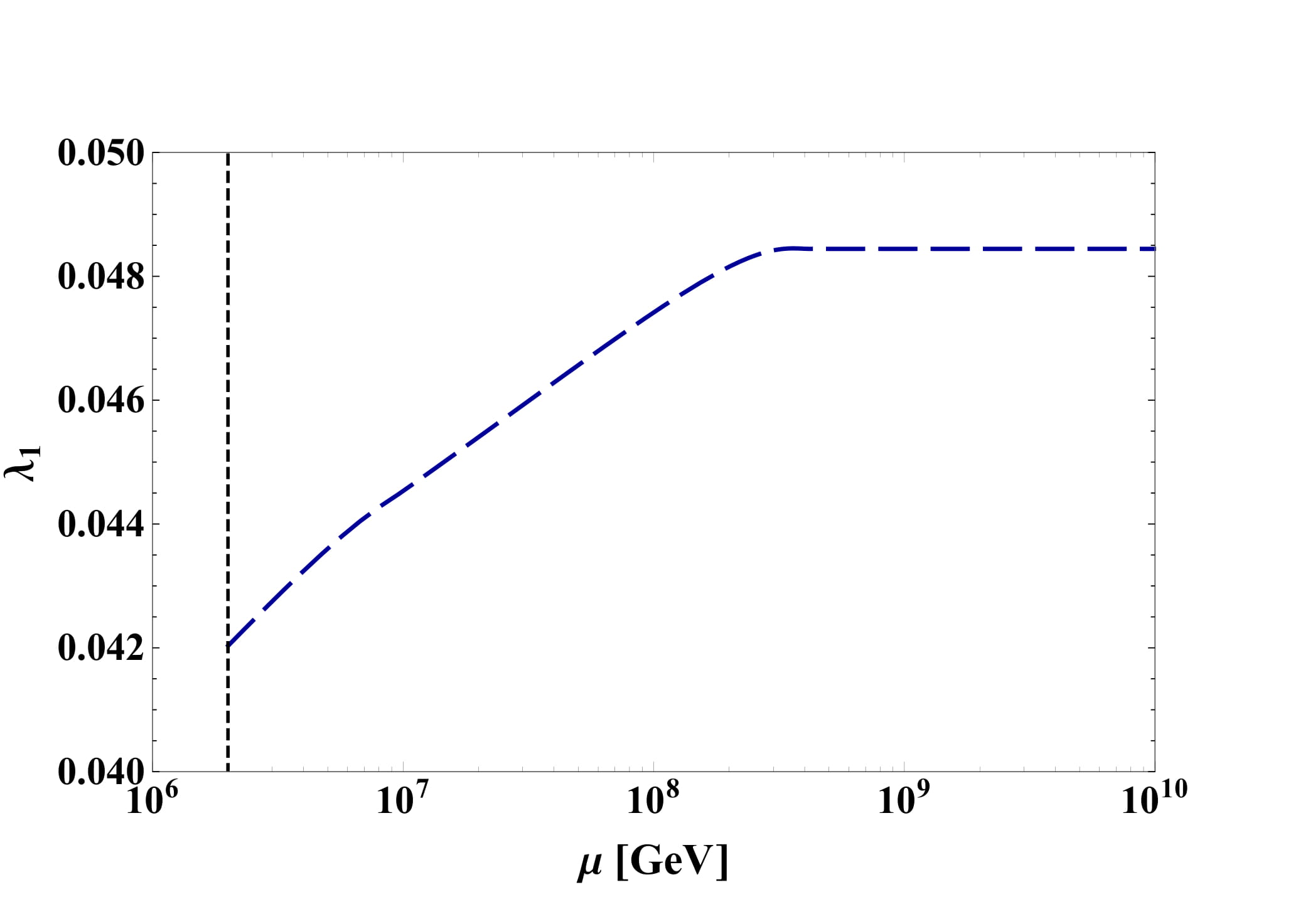
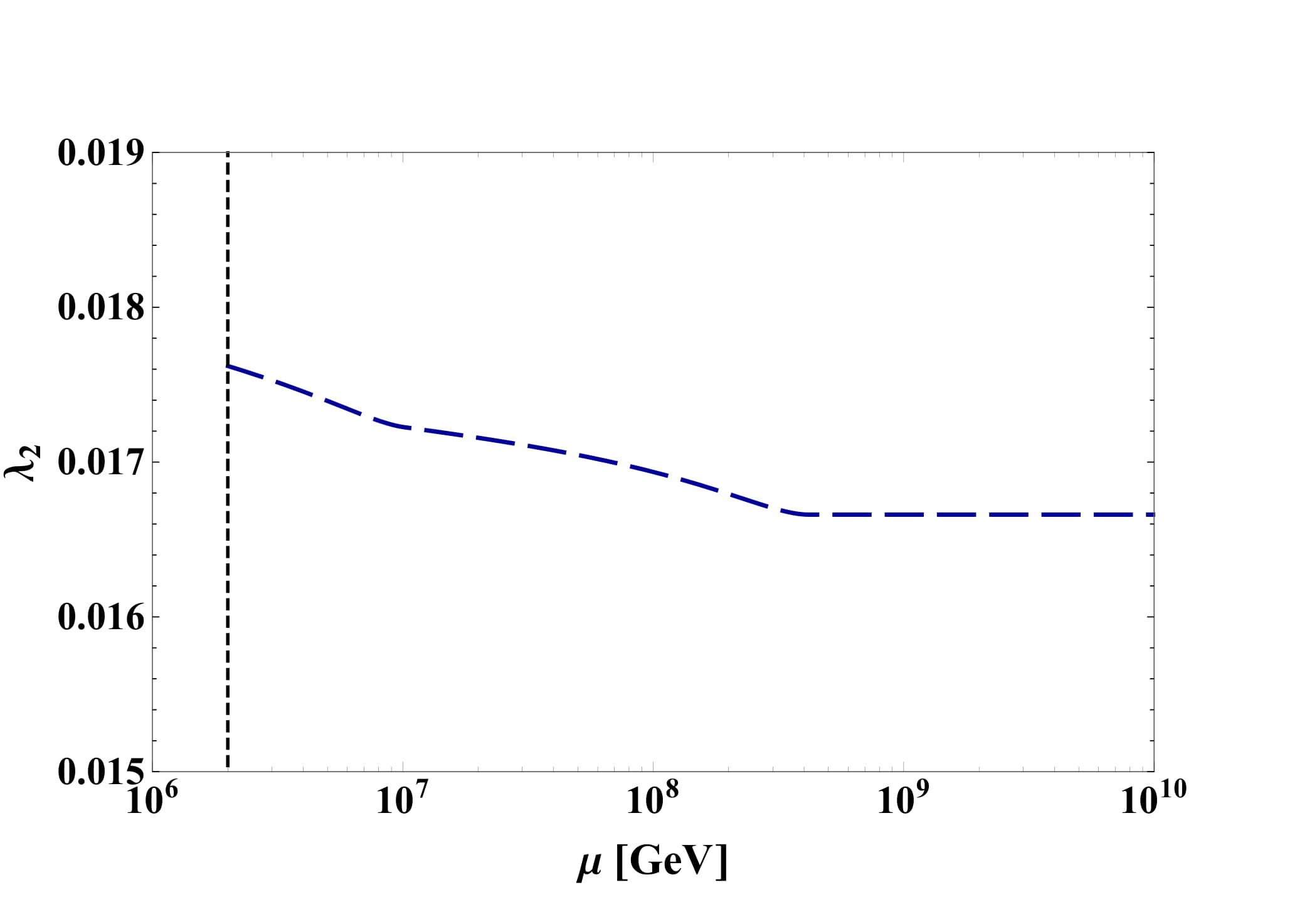
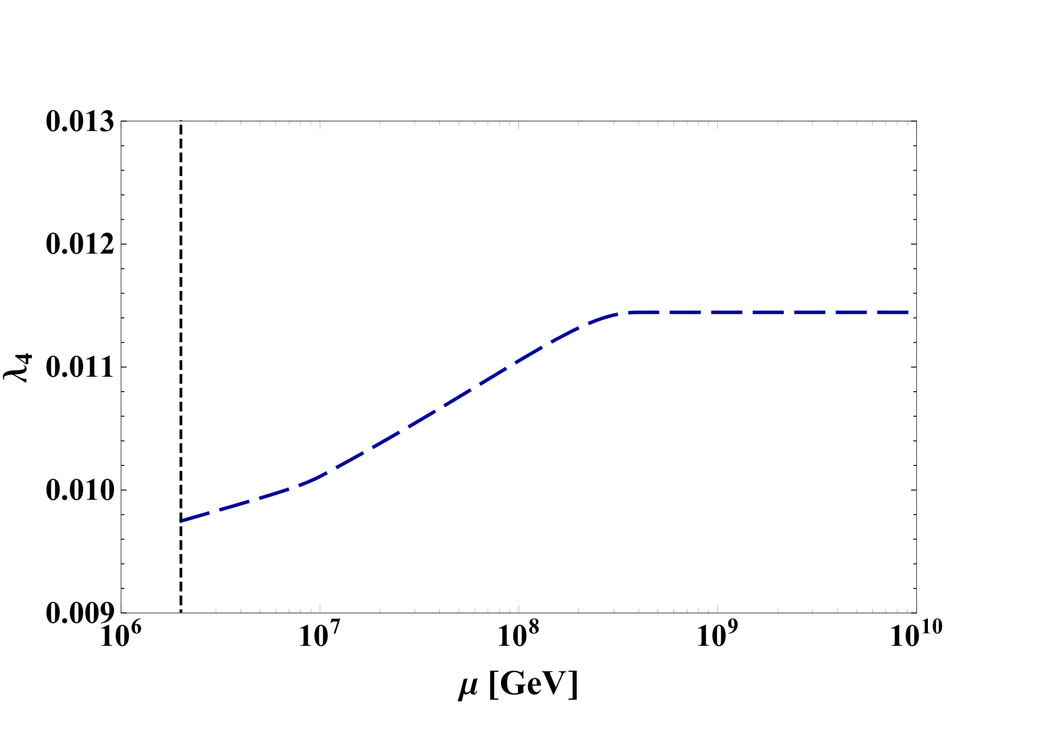
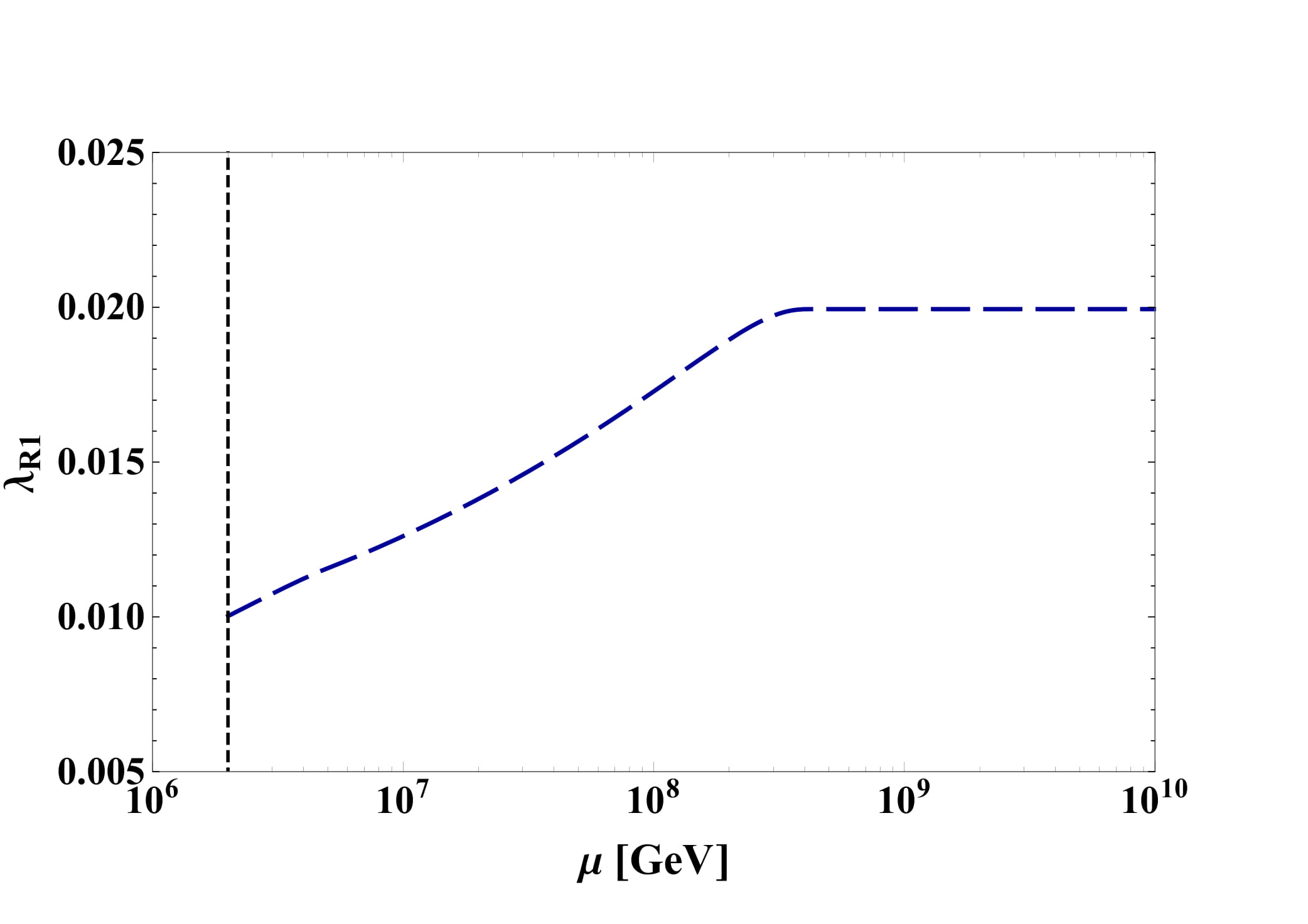
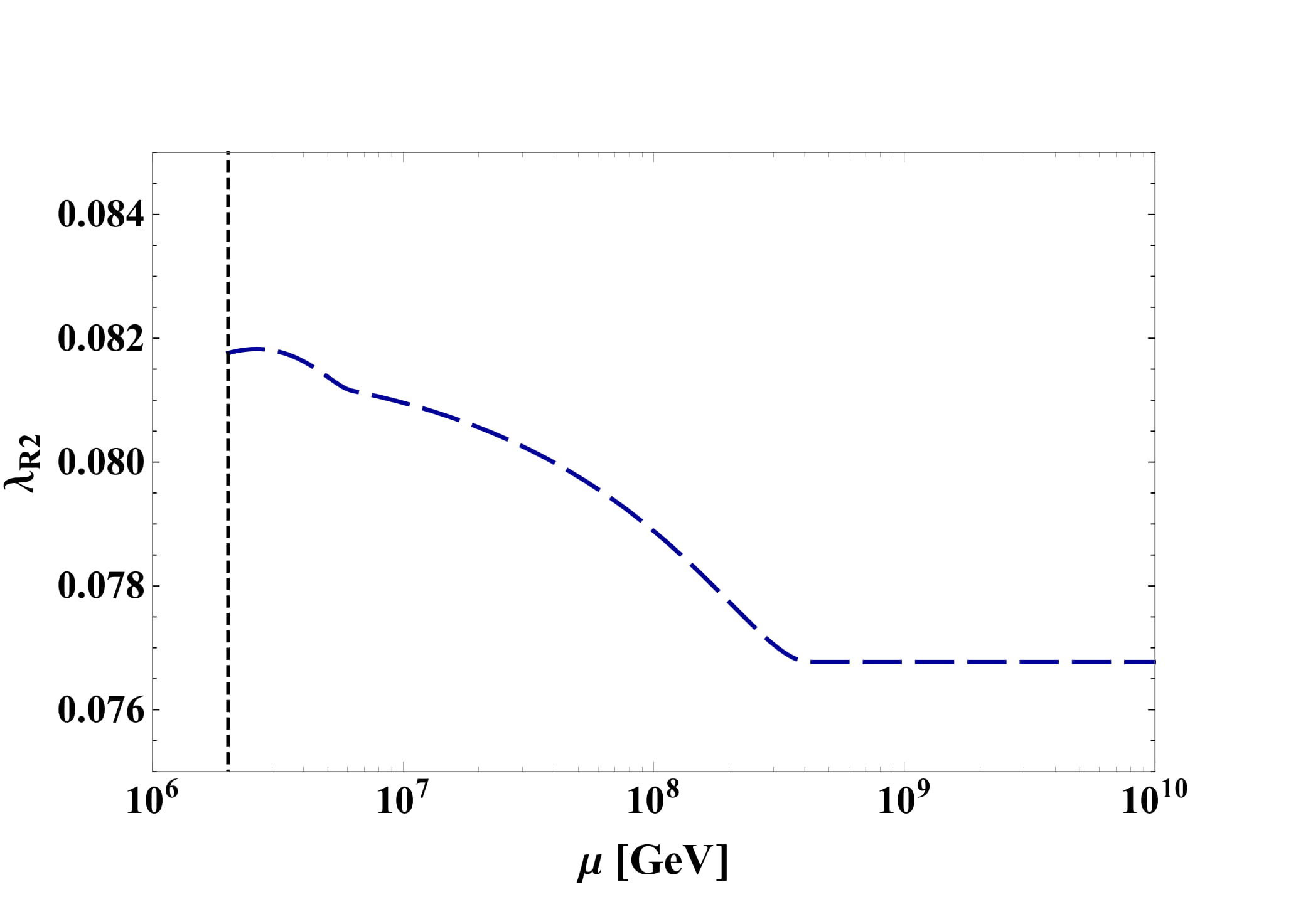
We report our results in Figs. 3 and 4 where we show the running of the gauge, Yukawa and scalar couplings by using the UV to IR approach for ($N_{F_{2L}}=40,\,N_{F_{2R}}=130,\,N_{F_{4}}=130$). The corresponding UV fixed point solution is the one shown in the AF row of Tab. 4. As mentioned above the RG flows of the gauge couplings are determined once the IR conditions are given. The IR initial conditions for $g_{L}$, $g_{R}$ and $g_{4}$ are obtained by using the matching conditions of Eq. (2) and Eq. (9) and the SM couplings are running from the EW scale to the Pati-Salam symmetry breaking scale. For simplicity, the vector-like fermions masses are taken to be the Pati-Salam symmetry breaking scale $v_{R}=2000\,\rm{TeV}$. From Figs. 3 and 4, it is clear that all couplings (i.e. gauge, Yukawa and scalar quartic) achieve a safe UV fixed point. The transition scale, above which, the UV fixed point is reached is about $0.5\times 10^{9}\,\rm{GeV}$ for all the couplings. Note that we could shift this transition scale significantly by increasing (the scale will decrease) or decreasing (the scale will increase) the number of vector-like fermions.

After Pati-Salam symmetry breaking, the scalar bi-doublet should match the conventional two Higgs doublet model which is defined by the Lagrangian:

$$\begin{split}V_{H}&=m_{11}^{2}\Phi_{1}^{\dagger}\Phi_{1}+m_{22}^{2}\Phi_{2}^{\dagger}\Phi_{2}-\left(m_{12}^{2}\Phi_{1}^{\dagger}\Phi_{2}+\rm{H.c.}\right)\\ &+\bar{\lambda}_{1}\left(\Phi_{1}^{\dagger}\Phi_{1}\right)^{2}+\bar{\lambda}_{2}\left(\Phi_{2}^{\dagger}\Phi_{2}\right)^{2}+\bar{\lambda}_{3}\left(\Phi_{1}^{\dagger}\Phi_{1}\right)\left(\Phi_{2}^{\dagger}\Phi_{2}\right)+\bar{\lambda}_{4}\left(\Phi_{1}^{\dagger}\Phi_{2}\right)\left(\Phi_{2}^{\dagger}\Phi_{1}\right)\\ &+\left[\frac{1}{2}\bar{\lambda}_{5}\left(\Phi_{1}^{\dagger}\Phi_{2}\right)^{2}+\bar{\lambda}_{6}\left(\Phi_{1}^{\dagger}\Phi_{1}\right)\left(\Phi_{1}^{\dagger}\Phi_{2}\right)+\bar{\lambda}_{7}\left(\Phi_{2}^{\dagger}\Phi_{2}\right)\left(\Phi_{1}^{\dagger}\Phi_{2}\right)+\rm{H.c.}\right]\,.\end{split}$$

(60)

Comparing (60) with (14), we find:

$$\begin{split}&\bar{\lambda}_{1}=\lambda_{1},\hskip 11.49994pt\bar{\lambda}_{2}=\lambda_{1},\hskip 11.49994pt\bar{\lambda}_{3}=2\lambda_{1},\hskip 11.49994pt\bar{\lambda}_{4}=4\left(-2\lambda_{2}+\lambda_{4}\right)\\ &\bar{\lambda}_{5}=4\lambda_{2},\hskip 11.49994pt\bar{\lambda}_{6}=-\lambda_{3},\hskip 11.49994pt\bar{\lambda}_{7}=\lambda_{3}\,.\end{split}$$

(61)

When a set of $\left(N_{F2},\,N_{F3},\,N_{F4}\right)$ is given and a Pati-Salam symmetry breaking pattern is chosen, by using the RG running from a specific UV fixed point, we could predict the coupling values at the Pati-Salam symmetry breaking scale. After implementing the matching conditions of Eq. (61) these couplings become our new initial values so that by employing the two Higgs doublet RG beta functions [55], we could obtain the coupling values at the electroweak scale.

References

- [1] D. F. Litim and F. Sannino, JHEP 1412, 178 (2014) doi:10.1007/JHEP12(2014)178 [arXiv:1406.2337 [hep-th]].
- [2] D. F. Litim, M. Mojaza and F. Sannino, JHEP 1601, 081 (2016) doi:10.1007/JHEP01(2016)081 [arXiv:1501.03061 [hep-th]].
- [3] F. Sannino, “ at LHC: Challenging asymptotic freedom,” arXiv:1511.09022 [hep-ph]. Invited contribution for [4].
- [4] D. d’Enterria et al., “Proceedings, High-Precision Measurements from LHC to FCC-ee : Geneva, Switzerland, October 2-13, 2015,” arXiv:1512.05194 [hep-ph].
- [5] S. Abel and F. Sannino, Phys. Rev. D 96, no. 5, 056028 (2017) doi:10.1103/PhysRevD.96.056028 [arXiv:1704.00700 [hep-ph]].
- [6] G. M. Pelaggi, F. Sannino, A. Strumia and E. Vigiani, Front. in Phys. 5, 49 (2017) doi:10.3389/fphy.2017.00049 [arXiv:1701.01453 [hep-ph]].
- [7] S. Abel and F. Sannino, Phys. Rev. D 96, no. 5, 055021 (2017) doi:10.1103/PhysRevD.96.055021 [arXiv:1707.06638 [hep-ph]].
- [8] A. D. Bond, G. Hiller, K. Kowalska and D. F. Litim, JHEP 1708, 004 (2017) doi:10.1007/JHEP08(2017)004 [arXiv:1702.01727 [hep-ph]].
- [9] K. Intriligator and F. Sannino, JHEP 1511, 023 (2015) doi:10.1007/JHEP11(2015)023 [arXiv:1508.07411 [hep-th]].
- [10] S. P. Martin and J. D. Wells, Phys. Rev. D 64, 036010 (2001) doi:10.1103/PhysRevD.64.036010 [hep-ph/0011382].
- [11] B. Bajc and F. Sannino, JHEP 1612, 141 (2016) doi:10.1007/JHEP12(2016)141 [arXiv:1610.09681 [hep-th]].
- [12] A. D. Bond and D. F. Litim, Phys. Rev. Lett. 119, no. 21, 211601 (2017) doi:10.1103/PhysRevLett.119.211601 [arXiv:1709.06953 [hep-th]].
- [13] B. Bajc, N. A. Dondi and F. Sannino, JHEP 1803, 005 (2018) doi:10.1007/JHEP03(2018)005 [arXiv:1709.07436 [hep-th]].
- [14] K. S. Babu, B. Bajc and S. Saad, arXiv:1805.10631 [hep-ph].
- [15] A. Palanques-Mestre and P. Pascual, Commun. Math. Phys. 95, 277 (1984). doi:10.1007/BF01212398
- [16] J. A. Gracey, Phys. Lett. B 373, 178 (1996) doi:10.1016/0370-2693(96)00105-0 [hep-ph/9602214].
- [17] B. Holdom, Phys. Lett. B 694, 74 (2011) doi:10.1016/j.physletb.2010.09.037 [arXiv:1006.2119 [hep-ph]].
- [18] C. Pica and F. Sannino, Phys. Rev. D 83, 035013 (2011) doi:10.1103/PhysRevD.83.035013 [arXiv:1011.5917 [hep-ph]].
- [19] R. Shrock, Phys. Rev. D 89, no. 4, 045019 (2014) doi:10.1103/PhysRevD.89.045019 [arXiv:1311.5268 [hep-th]].
- [20] F. Sannino and K. Tuominen, Phys. Rev. D 71, 051901 (2005) doi:10.1103/PhysRevD.71.051901 [hep-ph/0405209].
- [21] D. D. Dietrich and F. Sannino, Phys. Rev. D 75, 085018 (2007) doi:10.1103/PhysRevD.75.085018 [hep-ph/0611341].
- [22] F. Sannino, Acta Phys. Polon. B 40, 3533 (2009) [arXiv:0911.0931 [hep-ph]].
- [23] C. Pica, PoS LATTICE 2016, 015 (2016) doi:10.22323/1.256.0015 [arXiv:1701.07782 [hep-lat]].
- [24] O. Antipin and F. Sannino, Phys. Rev. D 97, no. 11, 116007 (2018) doi:10.1103/PhysRevD.97.116007 [arXiv:1709.02354 [hep-ph]].
- [25] K. Kowalska and E. M. Sessolo, JHEP 1804, 027 (2018) doi:10.1007/JHEP04(2018)027 [arXiv:1712.06859 [hep-ph]].
- [26] P. M. Ferreira, I. Jack and D. R. T. Jones, Phys. Lett. B 399, 258 (1997) doi:10.1016/S0370-2693(97)00291-8 [hep-ph/9702304].
- [27] P. M. Ferreira, I. Jack, D. R. T. Jones and C. G. North, Nucl. Phys. B 504, 108 (1997) doi:10.1016/S0550-3213(97)00448-3 [hep-ph/9705328].
- [28] G. M. Pelaggi, A. D. Plascencia, A. Salvio, F. Sannino, J. Smirnov and A. Strumia, Phys. Rev. D 97, no. 9, 095013 (2018) doi:10.1103/PhysRevD.97.095013 [arXiv:1708.00437 [hep-ph]].
- [29] O. Antipin, N. A. Dondi, F. Sannino, A. E. Thomsen and Z. W. Wang, arXiv:1803.09770 [hep-ph].
- [30] T. Alanne and S. Blasi, arXiv:1806.06954 [hep-ph].
- [31] R. Mann, J. Meffe, F. Sannino, T. Steele, Z. W. Wang and C. Zhang, Phys. Rev. Lett. 119, no. 26, 261802 (2017) doi:10.1103/PhysRevLett.119.261802 [arXiv:1707.02942 [hep-ph]].
- [32] J. McDowall and D. J. Miller, Phys. Rev. D 97, no. 11, 115042 (2018) doi:10.1103/PhysRevD.97.115042 [arXiv:1802.02391 [hep-ph]].
- [33] S. Ipek, A. D. Plascencia and J. Turner, arXiv:1806.00460 [hep-ph].
- [34] A. Eichhorn, A. Held and P. V. Griend, arXiv:1802.08589 [hep-ph].
- [35] A. Eichhorn, A. Held and C. Wetterich, Phys. Lett. B 782, 198 (2018) doi:10.1016/j.physletb.2018.05.016 [arXiv:1711.02949 [hep-th]].
- [36] M. Reichert, A. Eichhorn, H. Gies, J. M. Pawlowski, T. Plehn and M. M. Scherer, Phys. Rev. D 97, no. 7, 075008 (2018) doi:10.1103/PhysRevD.97.075008 [arXiv:1711.00019 [hep-ph]].
- [37] A. Eichhorn, S. Lippoldt and V. Skrinjar, Phys. Rev. D 97, no. 2, 026002 (2018) doi:10.1103/PhysRevD.97.026002 [arXiv:1710.03005 [hep-th]].
- [38] A. Eichhorn and F. Versteegen, JHEP 1801, 030 (2018) doi:10.1007/JHEP01(2018)030 [arXiv:1709.07252 [hep-th]].
- [39] H. Georgi and S. L. Glashow, Phys. Rev. Lett. 32, 438 (1974). doi:10.1103/PhysRevLett.32.438
- [40] J. C. Pati and A. Salam, Phys. Rev. D 10, 275 (1974) Erratum: [Phys. Rev. D 11, 703 (1975)]. doi:10.1103/PhysRevD.10.275, 10.1103/PhysRevD.11.703.2
- [41] P. Minkowski, Phys. Lett. 67B, 421 (1977). doi:10.1016/0370-2693(77)90435-X
- [42] T. Yanagida, Conf. Proc. C 7902131, 95 (1979).
- [43] M. Gell-Mann, P. Ramond and R. Slansky, Conf. Proc. C 790927, 315 (1979) [arXiv:1306.4669 [hep-th]].
- [44] R. N. Mohapatra and G. Senjanovic, Phys. Rev. Lett. 44, 912 (1980). doi:10.1103/PhysRevLett.44.912
- [45] R. R. Volkas, Phys. Rev. D 53, 2681 (1996) doi:10.1103/PhysRevD.53.2681 [hep-ph/9507215].
- [46] C. Pica and F. Sannino, Phys. Rev. D 83, 116001 (2011) doi:10.1103/PhysRevD.83.116001 [arXiv:1011.3832 [hep-ph]].
- [47] G. Valencia and S. Willenbrock, Phys. Rev. D 50, 6843 (1994) doi:10.1103/PhysRevD.50.6843 [hep-ph/9409201].
- [48] D. Ambrose et al. [BNL Collaboration], Phys. Rev. Lett. 81, 5734 (1998) doi:10.1103/PhysRevLett.81.5734 [hep-ex/9811038].
- [49] M. K. Parida, R. L. Awasthi and P. K. Sahu, JHEP 1501, 045 (2015) doi:10.1007/JHEP01(2015)045 [arXiv:1401.1412 [hep-ph]].
- [50] M. Holthausen, M. Lindner and M. A. Schmidt, Phys. Rev. D 82, 055002 (2010) doi:10.1103/PhysRevD.82.055002 [arXiv:0911.0710 [hep-ph]].
- [51] K. G. Wilson, Phys. Rev. B 4, 3174 (1971). doi:10.1103/PhysRevB.4.3174
- [52] K. G. Wilson, Phys. Rev. B 4, 3184 (1971). doi:10.1103/PhysRevB.4.3184
- [53] O. Antipin, M. Mojaza and F. Sannino, Phys. Rev. D 89, no. 8, 085015 (2014) doi:10.1103/PhysRevD.89.085015 [arXiv:1310.0957 [hep-ph]].
- [54] M. Shaposhnikov and A. Shkerin, arXiv:1804.06376 [hep-th].
- [55] G. C. Branco, P. M. Ferreira, L. Lavoura, M. N. Rebelo, M. Sher and J. P. Silva, Phys. Rept. 516 (2012) 1 [arXiv:1106.0034 [hep-ph]].
- [56] W. F. Chang, T. Modak and J. N. Ng, Phys. Rev. D 97 (2018) no.5, 055020 [arXiv:1711.05722 [hep-ph]].
- [57] G. Dupuis, JHEP 1607 (2016) 008 [arXiv:1604.04552 [hep-ph]].