Leptogenesis from oscillations and dark matter
Abstract
An extension of the Standard Model with Majorana singlet fermions in the 1-100 GeV range can explain the light neutrino masses and give rise to a baryon asymmetry at freeze-in of the heavy states, via their CP-violating oscillations. In this paper we consider extending this scenario to also explain dark matter. We find that a very weakly coupled gauge boson, an invisible QCD axion model, and the singlet majoron model can simultaneously account for dark matter and the baryon asymmetry.
I Introduction
The Standard Model (SM) of particle physics needs to be extended to explain neutrino masses, the missing gravitating matter (DM) and the observed matter-antimatter asymmetry in the universe.
Some of the most minimal extensions of the SM include new fermions, namely two or three sterile Majorana neutrinos (singlets under the full gauge group), which can account for the tiny neutrino masses, through the seesaw mechanism [1, 2, 3, 4], and explain the observed matter-antimatter asymmetry through leptogenesis [5]. The simplest version of leptogenesis establishes the source of the matter-antimatter asymmetry in the CP violating the out-of-equilibrium decay of the heavy neutrinos. This scenario requires however relatively large Majorana masses GeV [6] (or GeV with flavour effects [7] included), which makes these models difficult to test experimentally. For Majorana neutrinos in the 1-100 GeV range, it has been shown by Akhmedov, Rubakov and Smirnov (ARS) [8] and refined by Asaka and Shaposhnikov (AS) [9] that a different mechanism of leptogenesis is at work. In this case the asymmetries are produced at freeze-in of the sterile states via their CP-violating oscillations. The original ARS proposal did not include flavour effects and needs at least three Majorana species, while AS have shown that flavour effects can make it work with just two species. In the rest of the paper we will refer indistinctively to both scenarios as baryogenesis from oscillations (BO). In both cases, the lepton asymmetry is reprocessed into a baryonic one by electroweak sphalerons [10]. The extra heavy neutrinos in this case could be produced and searched for in beam dump experiments and colliders (see [11, 12, 13, 14, 15, 16, 17, 18, 19, 20, 21, 22, 23] for an incomplete list of works), possibly giving rise to spectacular signals such as displaced vertices [15, 16, 18, 20, 21]. Since only two sterile neutrinos are needed to generate the baryon asymmetry [9, 24, 25, 26, 27, 28, 29, 30, 31, 32, 33, 34, 35, 36, 37, 38, 39], the lightest sterile neutrino in the keV range can be very weakly coupled and play the role of DM [40]. This is the famous MSM [9]. However the stringent X-ray bounds imply that this scenario can only work in the presence of a leptonic asymmetry [41] significantly larger than the baryonic one, which is quite difficult to achieve. A recent update of astrophysical bounds on this scenario can be found in [42, 43]
In this paper our main goal is to consider scenarios compatible with Majorana masses in the 1-100 GeV range and study the conditions under which the models can explain DM without spoiling ARS leptogenesis 11 1 Some very recent work along these lines in the scotogenic model can be found in [120]. In particular, we will focus on models that are minimal extensions of the type I seesaw model with three singlet neutrinos. We will first consider an extension involving a gauged model [44], which includes an extra gauge boson and can explain DM in the form of a non-thermal keV neutrino. We will then consider an extension which includes a CP axion [45] that can solve the strong CP problem and explain DM in the form of cold axions. Finally we consider the majoron singlet model [46, 47] which can also explain DM under certain conditions both in the form of a heavy majorana neutrino or a majoron.
The plan of the paper is as follows. We start by briefly reviewing the ARS mechanism and the essential ingredients and conditions that need to be met when the sterile neutrinos have new interactions. In section III we discuss the gauged model, in section IV, we study the invisible axion model with sterile neutrinos and in section V we reconsider the singlet majoron model. In section VI we conclude.
II Leptogenesis from oscillations
For a recent extensive review of the ARS mechanism see [48]. The model is just the type I seesaw model with three neutrino singlets, , , which interact with the SM only through their Yukawa couplings. The Lagrangian in the Majorana mass basis is
| (1) |
In the early Universe before the electroweak (EW) phase transition, the singlet neutrinos are produced through their Yukawa couplings in flavour states, which are linear combinations of the mass eigenstates. Singlet neutrinos then oscillate, and since CP is not conserved, lepton number gets unevenly distributed between different flavours. At high enough temperatures , total lepton number vanishes, in spite of which a surplus of baryons over antibaryons can be produced, because the flavoured lepton asymmetries are stored in the different species and transferred at different rates to the baryons. As long as full equilibration of the sterile states is not reached before the EW phase transition (GeV) , when sphaleron processes freeze-out, a net baryon asymmetry survives. It is essential that at least one of the sterile neutrinos does not equilibrate by . The rate of interactions of these neutrinos at temperatures much higher than their mass can be estimated to be
| (2) |
where are the eigenvalues of the neutrino Yukawa matrix, is the temperature and few [49, 50, 51]. The Hubble expansion rate in the radiation dominated era is
| (3) |
where is the number of relativistic degrees of freedom ( above the EW phase transition). The requirement that no equilibration is reached before is:
| (4) |
which implies yukawa couplings of order
| (5) |
i.e. not much smaller than the electron yukawa. These yukawa couplings are compatible with the light neutrino masses for Majorana masses in the 1 GeV-100 GeV range.
Any model that extends the one described above with new fields/interactions should be such that the new interactions do not increase the equilibration rate of the sterile neutrinos for the out-of-equilibrium requirement in the ARS mechanism to be met. We will now consider the implications of this requirement on various extensions of the minimal seesaw model of eq. (1) that are well motivated by trying to explain also the dark matter and in one case also the strong CP problem.
III B-L gauge symmetry
The SM is invariant under an accidental global symmetry, that couples to baryon minus lepton number. If one promotes this symmetry to a local one [44], the model needs to be extended with three additional right handed neutrinos to avoid anomalies, which interestingly makes the type I seesaw model the minimal particle content compatible with this gauge symmetry. In this case, we have interactions between SM lepton and quark fields with the new gauge boson, , as well as an additional term involving sterile neutrinos
| (6) |
where for quarks and leptons respectively. We also assume the presence of a scalar field , with charge charge 2:
| (7) |
that gets an expectation value , breaking spontaneously 22 2 The Stuckelberg mechanism cannot be used here, because we need heavy neutrinos., and giving a mass to both the gauge boson and the sterile neutrinos:
| (8) |
A massive higgs from the breaking, , remains in the spectrum with a mass that we can assume to be .
Existing constraints on this model come from direct searches for in elastic neutrino-electron scattering, gauge boson production at colliders, Drell-Yan processes and new flavour changing meson decays [52, 53, 54, 55, 56, 57, 58, 59]. The status of these searches is summarized in Fig. 1, adapted from [60] (see also [61, 62, 63]). For masses, 1 GeV GeV, is bounded to be smaller than , while the limit is weaker for larger masses. The improved prospects to search for right-handed neutrinos exploiting the interaction have been recently studied in [60], where the authors consider the displaced decay of the at the LHC and the proposed SHIP beam dump experiment[64].


For GeV the strongest constraints come from supernova cooling [70, 71, 72, 67], beam dump searches [73, 69, 74, 75, 76, 77] and big bang nucleosynthesis (BBN)
[69, 68, 78, 79, 80]. Recent updates on these bounds are compiled in Fig. 2. The lower mass region labeled BBN is excluded by the effect of on the expansion, while the higher mass BBN region is excluded because the injection of electromagnetic energy from the decay to charged particles during nucleosynthesis distorts the abundance of light elements. These BBN constraints have been evaluated in detail in ref. [78, 79]. In the relevant region of parameter space, they are seen to depend on the lifetime of the decaying particle and its abundance per baryon prior to decay.
The corresponding region in Fig. 2 is a sketch of the excluded region in the latter analysis, which is approximately bounded by the lines corresponding to the lifetimes s, the threshold for hadronic decays, , and the line corresponding to the fraction of the decaying to charged particles per baryon, .
At least two of the neutrinos will be involved in the BO mechanism and their masses must be in the 1-100 GeV range. We need to ensure that the new interactions do not bring them to thermal equilibrium before , which will set an upper bound on . It it important to know however if the gauge boson is in thermal equilibrium which also depends on . For , the dominant process is the scattering with a rate that can be estimated to be
| (9) |
where is the Yukawa of the top quark and is its thermal mass. This rate is larger than the Hubble expansion somewhere above the EW transition provided . For larger masses of the gauge boson () the process kinematically opens up at high temperature and one has to consider the decay and inverse decay with a rate
where and for quarks(leptons). The sum is over all the standard model fermions whose thermal mass is such that . The lower limit on for the thermalization of the boson is shown as a dotted red line in Fig.1. Provided the boson is in thermal equilibrium we have to consider its interactions with the sterile neutrinos driving leptogenesis. Assuming that the boson is lighter than , so that the decay is kinematically forbidden, the dominant contribution [81] comes from the scattering processes with the fermions and gauge bosons in Fig.3. To ensure these processes do not equilibrate the sterile neutrinos, we should have
| (11) |
Assuming ,
| (12) |
and using eq. (8) we get
| (13) |
This upper bound is shown by the red solid line in Fig.1. In the next section we will include these new interactions in the equations for the generation of the baryon asymmetry, and our results confirm the naive estimate in eq. (13).


Finally we consider the production of neutrinos through the decay of , which is relevant for , since . The requirement that this process does not thermalize the sterile neutrinos implies that the decay rate, , is slower than the Hubble rate at :
| (14) |
For GeV, using eq. (8), we get
| (15) |
On the other hand, for the dominant production goes via the decay of the gauge boson into two sterile neutrinos , which, if kinematically allowed, scales with . In this case the decay rate is
| (16) |
Requiring that it is smaller than implies for
| (17) |
One may worry if thermal mass corrections can allow the decay at large temperatures even if . At high enough temperatures both sterile neutrinos and the gauge boson acquire thermal corrections to the masses of the form
| (18) |
The thermal mass of the gauge boson is larger than that of the sterile neutrino, because all fermions charged under will contribute to the former and only the gauge boson loop contributes to the later[82]:
| (19) |
We substitute the temperature dependent mass in eq. (16) and we show in Fig. 4 the ratio close to the minimum threshold temperature (where ), for and 100 GeV as a function of . The upper limit for are less stringent than those derived from processes in eq. (13).We now evaluate in detail the effect on BO induced by the new scatterings of Fig. 3. Leptogenesis in the presence of a new gauge interaction has been recently studied in [81], although not in the context of BO, which as far as we know has not been considered before.

III.1 Leptogenesis
The sterile neutrinos relevant for leptogenesis are the heavier ones, , with masses in the - GeV, and we focus on the scenario where . We now explain how to include the terms involving the gauge interactions in the quantum kinetic equations for BO leptogenesis as derived in [31]. Following Raffelt-Sigl approach [83], we consider a density matrix, , describing the expectation value of number densities of and a density matrix describing the corresponding anti-particles, 33 3 We can neglect Majorana masses in the range of masses considered and therefore particles and antiparticles correspond to the two helicity states. . These equations are complemented with three equations involving the slow varying chemical potentials, . The modification of the kinetic equations induced by the interactions is the addition of new collision terms in the equations for and , that have the same flavour structure as the neutral current contribution considered in [83]. As explained above the most relevant contributions come from the scattering processes: and . The latter is enhanced at high temperatures, but of course will only be relevant if the are in thermal equilibrium, which we assume in the following.
The additional collision terms, from the first process, in the equation for the evolution can be writen in the form:
| (20) |
where is the Fermi-Dirac equilibrium distribution function of the particle with momentum with ; is the anticommutator, and the normalized matrices are:
| (21) |
The additional collision terms for have the same form with the substitution .
For the second process we have similarly:
| (22) |
where is the equilibrium distribution function of the particle with momentum , ie. Bose-Einstein, , for and Fermi-Dirac, , for .
As usual we are interested in the evolution in an expanding universe, where the density matrices depend on momentum, and the scale factor or inverse temperature . We consider the averaged momentum approximation, which assumes that all the momentum dependence factorizes in the Fermi-Dirac distribution and the density is just a function of the scale factor, ie. . In this approximation we can do the integration over momentum and the terms in the equation for and become:
where is the Hubble expansion parameter.
The averaged rates including the two processes in eqs. (20) and (22) (assuming in the latter the are in equilibrium) are computed in the appendix with the result:
| (24) |
where the two terms inside the brackets correspond respectively to the and channels, and are valid for . Note the different temperature dependence of the two contributions. The growth of the at high temperatures originates in the contribution of the longitudinal polarization of the V bosons when the temperature is below the scalar mass, . For higher temperature, , the contribution of the physical scalar has to be included, leading to a rate . The new interactions do not modify the chemical potential dependent terms, nor the evolution equation for . The equations are therefore those in [31] with the additional terms in eq. ().
To illustrate the effect of the gauge interaction, we have considered the test point of ref. [31] with masses for the heavy steriles GeV. Within the parameter space of successful leptogenesis, this point was chosen because it leads to charmed meson decays to heavy sterile neutrinos that could be observable in SHIP, and furthermore this measurement, in combination with input from neutrinoless double beta decay and CP violation in neutrino oscillations, could provide a quantitative prediction of the baryon asymmetry. Adding the terms to the equations for and of [31], and solving them numerically (for details on the method see [31]) we obtain the curves in Fig. 5. The rates depend on so we choose GeV. The evolution of the baryon asymmetry as a function of is shown by the solid line of Fig. 5 in the absence of interactions or for a sufficiently small value of . The suppression of the asymmetry is visible for larger values of as shown by the dashed and dashed-dotted lines. The naive expectations in Fig. 1 is therefore confirmed and we do not expect a significant modification of the baryon asymmetry of the minimal model, as long as satisfies the bound in eq. (13).

III.2 Dark Matter
Now we want to discuss possible dark matter candidates in the scenario without spoiling the BO mechanism, which as we have seen imposes a stringent upper bound on the gauge coupling, . We will be interested in the region where the boson can decay to the lightest neutrino, ie . The small value needed for suggests to consider the possibility of a freeze-in scenario [84, 85], where the gauge boson does not reach thermalization, and neither does the lightest sterile neutrino, . The status of dark matter in a higher mass range through freeze-out has been recently updated in [63].
As it is well known, in the keV mass range is sufficiently long lived to provide a viable warm DM candidate [40, 41]. The model is as we will see a simple extension of the MSM [9], which avoids the need of huge lepton asymmetries to evade X-ray bounds. In our scenario the keV state is produced from the decay , while the lifetime of , relevant in X-ray bounds, is controlled also by mixing, which can be sufficiently small, in a technically natural way, as in the MSM scenario (provided the lightest neutrino mass is small enough). A similar scenario for DM has been studied in [66]. We now quantify the parameter space for successful DM and leptogenesis in this scenario.
We assume that the abundance of and is zero at a temperature below the EW phase transition where all the remaining particles in the model are in thermal equilibrium. All fermions in the model couple to the and therefore its production is dominated by the inverse decay process: . The kinetic equation describing the production of is the following:
| (25) |
where are the distribution function of the particle, , with momentum , and
| (26) |
is the number density, with the number of spin degrees of freedom. for a Dirac fermion, for a Majorana fermion and for a massive gauge boson. is the amplitude for the decay at tree level.
The sum over is over all fermions, but we can safely neglect the contribution of the and also those that are non-relativistic. We can also neglect the Pauli-blocking and stimulated emission effects () and approximate the distribution function in equilibrium for fermions and bosons by the Maxwell-Boltzmann, . Taking into account the relation
| (27) |
and the principle of detailed balance
| (28) |
the equation can be simplified to
| (29) |
As long as , the first term on the right-hand side can be neglected and the equation simplifies further to:
| (30) |
where is the first modified Bessel Function of the 2nd kind. The decay width in the rest frame is given by
where and for quarks(leptons).
As usual we define the yield of particle as
| (32) |
where is the entropy density
| (33) |
and we can assume . We also consider the averaged momentum approximation which amounts to assuming that has the same momentum dependence as . Changing variable from time to temperature, the final evolution equation for reads:
where .
The production of is dominated by the decay . There is also the contribution via mixing with the active neutrinos but this is negligible for mixings that evade present X ray bounds. Neglecting the inverse processes, the evolution equation for is
| (35) |
and in terms of the yield
where
| (37) |
It is straightforward to solve these equations. In Fig. 6 we show the yields of and as function of the inverse temperature for MeV, keV and .
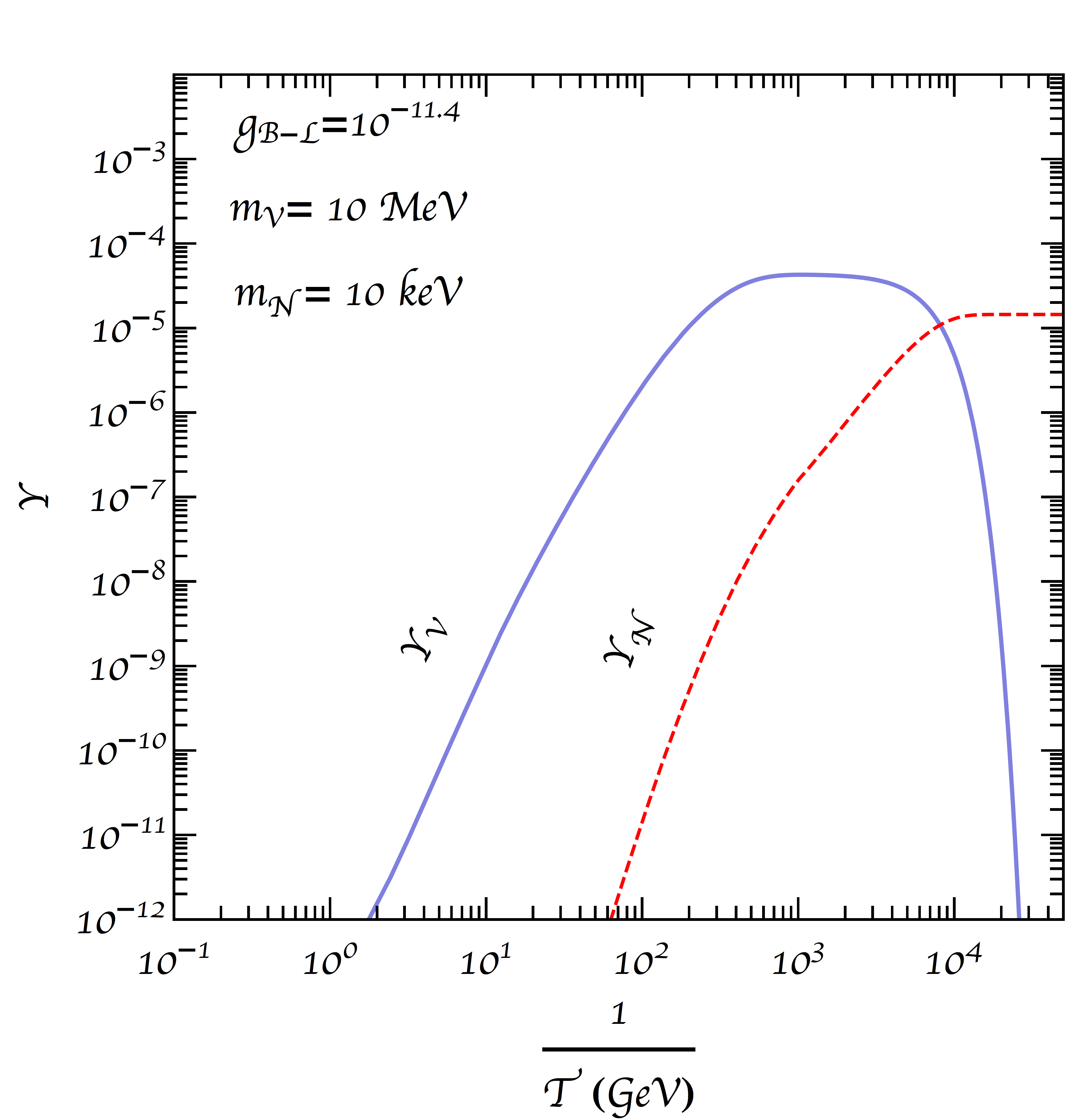
The resulting abundance of is
| (38) |
where = 2889.2 cm-3 is the entropy today and GeV cm-3 is the critical density. The evolution of is shown in Fig.7 for two values of and a fixed value of . Requiring that equals the full DM contribution of implies a relation between and as shown in the curves of Fig. 2.The values of corresponding to the right dark matter relic abundance do not affect leptogenesis and lie far below the actual collider limits. Nevertheless some regions of the parameter space are interestingly excluded from supernova and BBN observations.
A final comment concerns the comparison of our calculation of the DM abundance and that in ref. [66]. In this reference only the evolution of the is considered, and the collision term corresponds to the scattering process , where the narrow width approximation is assumed. We believe this method is only equivalent to ours when all and distributions are the equilibrium ones, but this is not the case here. In the region they can be compared our results are roughly a factor three smaller than those in [66].

III.3 Couplings
According to the previous calculation, the relic DM abundance requires a very small coupling. In order to obtain, for example, a mass MeV, the gauge coupling needed to generate DM is
| (39) |
and therefore
| (40) |
In order to get the and in the target range of keV and 1-100 GeV respectively, small and hierarchical couplings are needed:
| (41) |
for the heavy sterile neutrinos involved in BO leptogenesis and
| (42) |
for the dark matter candidate. Note that the required ’s couplings are in the same ballpark as the yukawa couplings. The gauged model works nicely to explain neutrino masses, the baryon asymmetry and dark matter. Unfortunately it also requires a very small which will be very hard to test experimentally. An alternative might be to consider a flavoured , for example , that might be compatible with a larger , provided the assignment of charges to the singlet states ensures that not all of them reach thermalization via the flavoured gauge interaction before .
IV Axion and Neutrinos
As a second example we consider an extension of eq. (1) with a scalar doublet and a scalar singlet. This model is also an extension of the invisible axion model [86] with sterile neutrinos, that was first considered in [45], providing a connection between the Peccei-Quinn (PQ) symmetry breaking scale and the seesaw scale of the neutrino masses. The model contains two scalar doublets, , and one singlet, . A global symmetry exists if the two Higgs doublets couple separately to the up and down quarks and leptons so that the Yukawa Lagrangian takes the form:
| (43) |
leading naturally to type II two-Higgs-doublet models without FCNC [87, 88].
The most general scalar potential of the model compatible with a global is the following
| (44) | |||||
The couplings in this potential can be chosen such that gets an expectation value,
| (45) |
is then spontaneously broken and a Nambu-Goldstone boson appears, the QCD axion. Furthermore the Majorana singlets get a mass. Expanding around the right vacuum, the field can be writen as
| (46) |
where is a massive field, while is the axion. Therefore after symmetry breaking we obtain an interaction term between sterile neutrinos and axions
| (47) |
The breaking scale must be much larger than the vacuum expectation values of the doublets, , so that the axion can evade the stringent bounds from rare meson decays and supernova cooling, which sets a stringent lower bound GeV [89].
The mass of the axion is induced by the QCD anomaly in the sub-eV range:
| (48) |
where . For GeV, we have
| (49) |
It is well known that the invisible axion is a viable cold DM candidate, through the misalignment mechanism [90, 86, 91] (for recent reviews see [92, 93]). The DM energy density is given by
| (50) |
where is the misalignment angle. The constraints on depend on whether the breaking of the PQ symmetry happens before or after inflation; in the latter case the misalignment angle can be averaged over many patches
| (51) |
so implies
| (52) |
with the equality reproducing the observed cold dark matter energy density . This correspond to the solid line in Fig. 8. If the PQ symmetry is broken before inflation, is a free parameter and the value of to account for DM is inversely proportional to .
The axion can also manifest itself as dark radiation [94], given that it is also thermally produced [95]. This population of hot axions contributes to the effective number of relativistic species, but the size of this contribution is currently well within the observational bounds [96].
In this model the VEV of the scalar singlet gives a Majorana mass to the sterile neutrinos:
| (53) |
So, if we want a mass in the electroweak range, GeV and GeV, we need the coupling to be in the range:
| (54) |
The hierarchy between and the electroweak scale requires that some couplings in the scalar potential in eq. (44) are very small. Even if not very appealing theoretically, these small numbers are technically natural as already pointed out in [97], where the authors studied the same model with very heavy sterile neutrinos.
A relevant question is that of naturalness or fine-tunning of the Higgs mass in this model. In [97], this issue was studied in the context of high-scale thermal leptogenesis, and it was concluded that stability imposes relevant constraints. In particular, a relatively small GeV is necessary to ensure viable leptogenesis for lower GeV so that yukawa’s are small enough, , and do not induce unnaturally large corrections to the Higgs mass.
In our case, the yukawa couplings, eq.(5), are too small to give large corrections to the Higgs mass , so no additional constraint needs to be imposed on . As a consequence other invisible axion models, such as the KSVZ [98, 99], would also work in the context of low-scale , but
leads to tension with stability bounds in the high-scale version [100, 101].

IV.1 Baryon Asymmetry
The possibility to generate the baryon asymmetry in this model a la Fukugita-Yanagida for very heavy neutrinos was recognized in the original proposal [45] and further elaborated in [97]. We want to point out here that for much smaller values of , the BO mechanism could also work successfully.
As explained above the crucial point is whether the new interactions of the sterile states in this model are fast enough to equilibrate all the sterile neutrinos before EW phase transition.
The leading order process we have to consider is the decay of the scalar into two sterile neutrinos , exactly as we considered in the previous section. The limit of GeV derived in eq. (15) also applies here, which is safely satisfied given the supernova cooling bounds.
At second order, we must also consider the new annihilation process of sterile neutrinos to axions as shown in Fig. 9. The rate of this process at high temperatures, , is given by
| (55) |
The condition is satisfied for if
| (56) |
(for GeV), safely within the targeted range. Fig.8 shows the region on the plane for which successful baryogenesis through the BO mechanism and DM can work in this model.

Even if the necessary condition for BO leptogenesis is met for GeV, the presence of the extra degrees of freedom, the axion, the heavy scalar and the second doublet could modify quantitatively the baryon asymmetry. For example, the presence of two scalar doublets could modify the scattering rates of the sterile neutrinos considered in the BO scenario, where the main contributions [102, 49, 51, 35] are:
- •
scatterings on top quarks via higgs exchange
- •
scatterings on gauge bosons
- •
decays or inverse decays including resumed soft-gauge interactions
Sterile neutrinos are coupled to the same Higgs doublet that also couples to the top quarks; in this case nothing changes with respect to the usual calculation, in which the reactions with top quarks are mediated by .
However, an alternative model, with a different charge assignment, is also possible, in which the sterile neutrinos couple to and not , as done in
[97].
In this case top quark scattering does not contribute to sterile neutrino production at tree level, but the baryon asymmetry is not expected to change significantly, since the scattering rate on gauge bosons and the 1 2 processes are equally important [49, 51].
The process is not foreseen to be relevant for , since the scalar is long decoupled when the generation of the asymmetry starts, while the new process is expected to be very small according to the above estimates. It could nevertheless be interesting to look for possible corners of parameter space where the differences with respect to the minimal model is not negligible since this could provide a testing ground for the axion sector of the model.
V Majoron model
In between the two models described in III - IV, there is the possibility of having a global spontaneously broken, which is not related to the strong CP problem and we call it lepton number. This is of course the well-known singlet majoron model [46, 47, 103]. We assume the sterile neutrinos carry lepton number, , but Majorana masses are forbidden and replaced by a yukawa interaction as in the model:
| (57) |
where is the standard model Higgs doublet, while is a complex scalar which carries lepton number . Then, the complex scalar acquires a VEV
| (58) |
and the is spontaneously broken giving rise to the right-handed Majorana mass matrix and leading to a Goldstone boson , the majoron. Consequently the Lagrangian will induce the new scattering processes for neutrinos depicted in Fig. 9.
As usual we have to ensure that at least one sterile neutrino does not equilibrate before (see [104, 105] for a recent discussion in the standard high-scale or resonant leptogenesis). As in the previous cases we have to consider the decay and the annihilation into majorons, Fig. 9. The former gives the strongest constraint, as in eq. (15):
| (59) |
These lower bounds for and 100 GeV are shown by the horizontal lines in Fig. 10.
V.1 Dark Matter
There are two candidates in this model for dark matter that we consider in turn: the Majoron and the lightest sterile neutrino, .
V.1.1 Majoron
In this model a natural candidate for dark matter is the majoron itself, but it has to acquire a mass, therefore becoming a pseudo Nambu-Goldstone boson (pNGB). One possibility is to appeal to gravitational effects [106, 107]. However, the contribution to the mass from gravitational instantons is estimated to be [108, 109, 110]
| (60) |
and therefore extremely tiny, unless is close to the Planck scale.
Another alternative is to consider a flavoured and soft symmetry breaking terms in the form of yukawa couplings [111, 112]. This possibility has been studied in detail in ref. [112]. It has been shown that the majoron can be the main component of dark matter for sterile neutrino masses GeV, while for masses in the range we are interested in ( GeV) neither thermal production via freeze-out nor via freeze-in works.
The possibility to produce it via vacuum misalignment, analogous to the one which produces the axion relic density has also been discussed in [112]. It was shown to give a negligible contribution compared to the thermal one, because the majoron gets a temperature dependent mass at early times. Even if the mass of the majoron is significantly smaller in our situation, with lighter , we find the same result, ie. that only a small fraction of the DM can be produced via misalignmet.
No matter what the production mechanism is if the majoron constitutes the dark matter, there are constraints from the requirement that the majoron be stable on a cosmological timescale and its decay to the light neutrinos
| (61) |
should not spoil the CMB anisotropy spectrum[113, 114]. This gives constraints on the mass and the symmetry breaking scale , as showed in Fig.10

As in the axion case there are additional constraints from supernova cooling [115], but they are much weaker and give an upper bound much lower than the range shown in Fig. 10. In the unconstrained region in Fig. 10, ARS leptogenesis and majoron DM could in principle work provided the mechanism to generate the majoron mass does not involve further interactions of the sterile neutrinos.
V.1.2 Sterile Neutrino
We want now to consider the sterile neutrino as a dark matter candidate, a possibility already explored in [116, 117] in a model with a real scalar field and therefore no Majoron. In our case the presence of the Majoron could make the sterile neutrino unstable, given that it would decay through the channel
| (62) |
Thus one has to assume that the Majoron has a larger mass so that this decay is kinematically forbidden.
As in the case, BO leptogenesis is driven by the other two heavier neutrino states , while can be produced through freeze-in from decay. Assuming is in thermal equilibrium with the bath the Boltzmann equation describing the evolution of the density:
| (63) |
where we have neglected Pauli blocking, and the inverse processes.
Following the standard procedure we end with the contribution to the abundance:
| (64) |
Using
| (65) |
and requiring that matches the observed DM we find
| (66) |
The mass of the DM candidate is related to the coupling which regulates the freeze-in process through the VEV of
| (67) |
therefore if , the coupling needs to be
| (68) |
as shown in Fig. 11.

If is the keV range so that it can satisfy cosmological and astrophysical constraints, the scale of the VEV should be
| (69) |
As a consequence we see that if one couples the scalar also to the heavier neutrinos, the interactions are too fast and the BO mechanism cannot work since the bound in eq. (59) is not satisfied. Alternatively, if we assume eq. (59), then
| (70) |
Such a massive neutrino would need extremely small active-sterile mixing angle (collectively labeled ) to be sufficiently long-lived. The strongest bound from X-rays [118] give
| (71) |
while the soft gamma ray bound [119] gives
| (72) |
In conclusion, either we consider a global symmetry with different family charges, more concretely a , or we need to require extremely tiny yukawa coupling for the DM sterile neutrino, making this last model theoretically unappealing.
VI Conclusion
The extension of the Standard Model with three heavy majorana singlets at the weak scale can explain neutrino masses and also account for the baryon asymmetry in the Universe via the oscillation mechanism [8, 9]. This scenario could be testable in future experiments.
Unfortunately the simplest model cannot easily accommodate dark matter. In the MSM [9], one of the three heavy states is in the keV range and provides a candidate for dark matter, but it requires huge lepton asymmetries that cannot be naturally achieved in the minimal setup.
In this paper we have explored three extensions of the minimal scenario that
can accommodate dark matter without spoiling baryogenesis. This is non trivial because new interactions of the heavy singlets can disrupt the necessary out-of-equilibrium condition
which is mandatory to generate a lepton asymmetry. We have shown that a extension of the minimal model with a gauge interaction can achieve this goal. The two heavier majorana fermions take part in the generation of the baryon asymmetry, while the lighest one in the keV range, , is the dark matter. In contrast with the MSM the production
of the dark matter is not via mixing, but it is dominated by the gauge boson decay. The mixing is however what controls the decay of the and can be made
sufficiently small to avoid the stringent X-ray constraints. The correct DM abundance is achieved for very small gauge couplings, , which are safely small not to disturb the baryon asymmetry, which remains the same as in the minimal model. Such tiny couplings are far below the reach of colliders. Supernova and BBN
provide the most stringent constraints in the relevant region of parameter space, while future searches in SHIP might have a chance to touch on it.
We have also considered an extension involving an invisible axion sector with an extra scalar doublet and a complex singlet. The heavy majorana singlets get their mass from the PQ breaking scale [45]. DM is in the form of cold axions, from the misalignment mechanism and as is well known, the right relic abundance can be achieved for a large value of the PQ breaking scale, GeV. We have shown that such large scale is compatible with having the heavy neutrinos in the 1-100 GeV scale, and ARS leptogenesis. Finally we have considered the singlet majoron extension of the minimal model, with a global , that contains two potential DM candidates, the majoron or the lightest heavy neutrino, . Unperturbed ARS baryogenesis requires a relatively high breaking scale, GeV. Majoron DM requires exotic production scenarios, while neutrino DM works for masses around MeV, which requires extremely small mixings to make it sufficiently long-lived, or alternatively a less theoretically appealing possibity, where
the scalar couples to only one sterile neutrino, while the other two have tree level masses or couple to a different scalar with a larger VEV.
As a general rule, adding new interactions that affect the heavy Majorana singlets modifies leptogenesis in the minimal model and viable extensions that can explain DM
are likely to involve the freeze-in mechanism as in the examples above.
Acknowledgements
We thank M. Escudero, M. Kekic, J. López-Pavón and J. Salvado for useful discussions. We acknowledge support from national grants FPA2014-57816-P, FPA2017-85985-P and the European projects H2020-MSCA-ITN-2015//674896-ELUSIVES and H2020-MSCA-RISE-2015
Appendix A Computation of momentum averaged rates in gauged
In this appendix we give some details on the computation of the momentum averaged rates in eq. (24). The amplitude for for vanishing masses is given by
while that for , in the limit is
| (74) |
Defining the Bose-Einstein and Fermi-Dirac distributions
| (75) |
and the variables
| (76) |
where . We express all momenta in units of temperature .
Following the procedure of ref. [49] the rate can be writen as
| (77) |
with
| (78) |
| (79) |
| (80) |
with
| (81) |
and
| (82) |
| (83) |
The rate can be written as
| (84) |
with
| (85) |
and .
The total rate is
| (86) |
and the averaged rates and are found to be:
| (87) |
| (88) |
where
| (89) |
and
| (90) |
References
- [1] P. Minkowski, Phys. Lett. 67B, 421 (1977).
- [2] M. Gell-Mann, P. Ramond, and R. Slansky, Conf. Proc. C790927, 315 (1979), eprint 1306.4669.
- [3] T. Yanagida, Conf. Proc. C7902131, 95 (1979).
- [4] R. N. Mohapatra and G. Senjanovic, Phys. Rev. Lett. 44, 912 (1980).
- [5] M. Fukugita and T. Yanagida, Phys. Lett. B174, 45 (1986).
- [6] S. Davidson and A. Ibarra, Phys. Lett. B535, 25 (2002), eprint hep-ph/0202239.
- [7] A. Abada, S. Davidson, A. Ibarra, F. X. Josse-Michaux, M. Losada, and A. Riotto, JHEP 09, 010 (2006), eprint hep-ph/0605281.
- [8] E. K. Akhmedov, V. A. Rubakov, and A. Yu. Smirnov, Phys. Rev. Lett. 81, 1359 (1998), eprint hep-ph/9803255.
- [9] T. Asaka and M. Shaposhnikov, Phys. Lett. B620, 17 (2005), eprint hep-ph/0505013.
- [10] V. A. Kuzmin, V. A. Rubakov, and M. E. Shaposhnikov, Phys. Lett. 155B, 36 (1985).
- [11] A. Ferrari, J. Collot, M.-L. Andrieux, B. Belhorma, P. de Saintignon, J.-Y. Hostachy, P. Martin, and M. Wielers, Phys. Rev. D62, 013001 (2000).
- [12] M. L. Graesser (2007), eprint 0705.2190.
- [13] F. del Aguila and J. A. Aguilar-Saavedra, Nucl. Phys. B813, 22 (2009), eprint 0808.2468.
- [14] P. S. Bhupal Dev, R. Franceschini, and R. N. Mohapatra, Phys. Rev. D86, 093010 (2012), eprint 1207.2756.
- [15] J. C. Helo, M. Hirsch, and S. Kovalenko, Phys. Rev. D89, 073005 (2014), [Erratum: Phys. Rev.D93,no.9,099902(2016)], eprint 1312.2900.
- [16] A. Blondel, E. Graverini, N. Serra, and M. Shaposhnikov (FCC-ee study Team), Nucl. Part. Phys. Proc. 273-275, 1883 (2016), eprint 1411.5230.
- [17] A. Abada, V. De Romeri, S. Monteil, J. Orloff, and A. M. Teixeira, JHEP 04, 051 (2015a), eprint 1412.6322.
- [18] Y. Cui and B. Shuve, JHEP 02, 049 (2015), eprint 1409.6729.
- [19] S. Antusch and O. Fischer, JHEP 05, 053 (2015), eprint 1502.05915.
- [20] A. M. Gago, P. Hernandez, J. Jones-Perez, M. Losada, and A. Moreno Briceño, Eur. Phys. J. C75, 470 (2015), eprint 1505.05880.
- [21] S. Antusch, E. Cazzato, and O. Fischer, JHEP 12, 007 (2016), eprint 1604.02420.
- [22] A. Caputo, P. Hernandez, M. Kekic, J. Lopez-Pavon, and J. Salvado, Eur. Phys. J. C77, 258 (2017a), eprint 1611.05000.
- [23] A. Caputo, P. Hernandez, J. Lopez-Pavon, and J. Salvado, JHEP 06, 112 (2017b), eprint 1704.08721.
- [24] M. Shaposhnikov, JHEP 08, 008 (2008), eprint 0804.4542.
- [25] L. Canetti, M. Drewes, and M. Shaposhnikov, New J. Phys. 14, 095012 (2012), eprint 1204.4186.
- [26] L. Canetti, M. Drewes, T. Frossard, and M. Shaposhnikov, Phys. Rev. D87, 093006 (2013), eprint 1208.4607.
- [27] T. Asaka, S. Eijima, and H. Ishida, JCAP 1202, 021 (2012), eprint 1112.5565.
- [28] B. Shuve and I. Yavin, Phys. Rev. D89, 075014 (2014), eprint 1401.2459.
- [29] A. Abada, G. Arcadi, V. Domcke, and M. Lucente, JCAP 1511, 041 (2015b), eprint 1507.06215.
- [30] P. Hernandez, M. Kekic, J. Lopez-Pavon, J. Racker, and N. Rius, JHEP 10, 067 (2015), eprint 1508.03676.
- [31] P. Hernandez, M. Kekic, J. Lopez-Pavon, J. Racker, and J. Salvado, JHEP 08, 157 (2016), eprint 1606.06719.
- [32] M. Drewes, B. Garbrecht, D. Gueter, and J. Klaric, JHEP 12, 150 (2016), eprint 1606.06690.
- [33] M. Drewes, B. Garbrecht, D. Gueter, and J. Klaric, JHEP 08, 018 (2017), eprint 1609.09069.
- [34] T. Hambye and D. Teresi, Phys. Rev. Lett. 117, 091801 (2016), eprint 1606.00017.
- [35] J. Ghiglieri and M. Laine, JHEP 05, 132 (2017), eprint 1703.06087.
- [36] T. Asaka, S. Eijima, H. Ishida, K. Minogawa, and T. Yoshii (2017), eprint 1704.02692.
- [37] T. Hambye and D. Teresi, Phys. Rev. D96, 015031 (2017), eprint 1705.00016.
- [38] A. Abada, G. Arcadi, V. Domcke, and M. Lucente, JCAP 1712, 024 (2017), eprint 1709.00415.
- [39] J. Ghiglieri and M. Laine, JHEP 02, 078 (2018), eprint 1711.08469.
- [40] S. Dodelson and L. M. Widrow, Phys. Rev. Lett. 72, 17 (1994), eprint hep-ph/9303287.
- [41] X.-D. Shi and G. M. Fuller, Phys. Rev. Lett. 82, 2832 (1999), eprint astro-ph/9810076.
- [42] K. Perez, K. C. Y. Ng, J. F. Beacom, C. Hersh, S. Horiuchi, and R. Krivonos, Phys. Rev. D95, 123002 (2017), eprint 1609.00667.
- [43] J. Baur, N. Palanque-Delabrouille, C. Yeche, A. Boyarsky, O. Ruchayskiy, Ã. Armengaud, and J. Lesgourgues, JCAP 1712, 013 (2017), eprint 1706.03118.
- [44] R. N. Mohapatra and R. E. Marshak, Phys. Rev. Lett. 44, 1316 (1980), [Erratum: Phys. Rev. Lett.44,1643(1980)].
- [45] P. Langacker, R. D. Peccei, and T. Yanagida, Mod. Phys. Lett. A1, 541 (1986).
- [46] Y. Chikashige, R. N. Mohapatra, and R. D. Peccei, Phys. Lett. 98B, 265 (1981).
- [47] J. Schechter and J. W. F. Valle, Phys. Rev. D25, 774 (1982).
- [48] M. Drewes, B. Garbrecht, P. Hernandez, M. Kekic, J. Lopez-Pavon, J. Racker, N. Rius, J. Salvado, and D. Teresi, Int. J. Mod. Phys. A33, 1842002 (2018), eprint 1711.02862.
- [49] D. Besak and D. Bodeker, JCAP 1203, 029 (2012), eprint 1202.1288.
- [50] B. Garbrecht, F. Glowna, and P. Schwaller, Nucl. Phys. B877, 1 (2013), eprint 1303.5498.
- [51] I. Ghisoiu and M. Laine, JCAP 1412, 032 (2014), eprint 1411.1765.
- [52] G. Bellini et al., Phys. Rev. Lett. 107, 141302 (2011), eprint 1104.1816.
- [53] S. Chatrchyan et al. (CMS), JHEP 12, 030 (2013), eprint 1310.7291.
- [54] J. P. Lees et al. (BaBar), Phys. Rev. Lett. 113, 201801 (2014), eprint 1406.2980.
- [55] J. P. Lees et al. (BaBar), Phys. Rev. Lett. 119, 131804 (2017), eprint 1702.03327.
- [56] V. Khachatryan et al. (CMS), JHEP 04, 025 (2015), eprint 1412.6302.
- [57] G. Aad et al. (ATLAS), Phys. Rev. D90, 052005 (2014), eprint 1405.4123.
- [58] (2004), eprint hep-ex/0412015.
- [59] T. Appelquist, B. A. Dobrescu, and A. R. Hopper, Phys. Rev. D68, 035012 (2003), eprint hep-ph/0212073.
- [60] B. Batell, M. Pospelov, and B. Shuve, JHEP 08, 052 (2016), eprint 1604.06099.
- [61] M. Klasen, F. Lyonnet, and F. S. Queiroz, Eur. Phys. J. C77, 348 (2017), eprint 1607.06468.
- [62] P. Ilten, Y. Soreq, M. Williams, and W. Xue, JHEP 06, 004 (2018), eprint 1801.04847.
- [63] M. Escudero, S. J. Witte, and N. Rius (2018), eprint 1806.02823.
- [64] S. Alekhin et al., Rept. Prog. Phys. 79, 124201 (2016), eprint 1504.04855.
- [65] D. Gorbunov, A. Makarov, and I. Timiryasov, Phys. Rev. D91, 035027 (2015), eprint 1411.4007.
- [66] K. Kaneta, Z. Kang, and H.-S. Lee, JHEP 02, 031 (2017), eprint 1606.09317.
- [67] J. H. Chang, R. Essig, and S. D. McDermott, JHEP 01, 107 (2017), eprint 1611.03864.
- [68] B. Ahlgren, T. Ohlsson, and S. Zhou, Phys. Rev. Lett. 111, 199001 (2013), eprint 1309.0991.
- [69] M. Williams, C. P. Burgess, A. Maharana, and F. Quevedo, JHEP 08, 106 (2011), eprint 1103.4556.
- [70] R. Mayle, J. R. Wilson, J. R. Ellis, K. A. Olive, D. N. Schramm, and G. Steigman, Phys. Lett. B203, 188 (1988).
- [71] G. Raffelt and D. Seckel, Phys. Rev. Lett. 60, 1793 (1988).
- [72] M. S. Turner, Phys. Rev. Lett. 60, 1797 (1988).
- [73] J. D. Bjorken, R. Essig, P. Schuster, and N. Toro, Phys. Rev. D80, 075018 (2009), eprint 0906.0580.
- [74] P. Vilain et al. (CHARM-II), Phys. Lett. B302, 351 (1993).
- [75] J. D. Bjorken, S. Ecklund, W. R. Nelson, A. Abashian, C. Church, B. Lu, L. W. Mo, T. A. Nunamaker, and P. Rassmann, Phys. Rev. D38, 3375 (1988).
- [76] E. M. Riordan et al., Phys. Rev. Lett. 59, 755 (1987).
- [77] A. Bross, M. Crisler, S. H. Pordes, J. Volk, S. Errede, and J. Wrbanek, Phys. Rev. Lett. 67, 2942 (1991).
- [78] A. Fradette, M. Pospelov, J. Pradler, and A. Ritz, Phys. Rev. D90, 035022 (2014), eprint 1407.0993.
- [79] J. Berger, K. Jedamzik, and D. G. E. Walker, JCAP 1611, 032 (2016), eprint 1605.07195.
- [80] G.-y. Huang, T. Ohlsson, and S. Zhou, Phys. Rev. D97, 075009 (2018), eprint 1712.04792.
- [81] J. Heeck and D. Teresi, Phys. Rev. D94, 095024 (2016), eprint 1609.03594.
- [82] H. A. Weldon, Phys. Rev. D26, 2789 (1982).
- [83] G. Sigl and G. Raffelt, Nucl. Phys. B406, 423 (1993).
- [84] J. McDonald, Phys. Rev. Lett. 88, 091304 (2002), eprint hep-ph/0106249.
- [85] L. J. Hall, K. Jedamzik, J. March-Russell, and S. M. West, JHEP 03, 080 (2010), eprint 0911.1120.
- [86] M. Dine and W. Fischler, Phys. Lett. B120, 137 (1983).
- [87] G. C. Branco, P. M. Ferreira, L. Lavoura, M. N. Rebelo, M. Sher, and J. P. Silva, Phys. Rept. 516, 1 (2012), eprint 1106.0034.
- [88] D. Espriu, F. Mescia, and A. Renau, Phys. Rev. D92, 095013 (2015), eprint 1503.02953.
- [89] G. G. Raffelt, Ann. Rev. Nucl. Part. Sci. 49, 163 (1999), eprint hep-ph/9903472.
- [90] J. Preskill, M. B. Wise, and F. Wilczek, Phys. Lett. B120, 127 (1983).
- [91] L. F. Abbott and P. Sikivie, Phys. Lett. B120, 133 (1983).
- [92] M. Kawasaki and K. Nakayama, Ann. Rev. Nucl. Part. Sci. 63, 69 (2013), eprint 1301.1123.
- [93] D. J. E. Marsh, Phys. Rept. 643, 1 (2016), eprint 1510.07633.
- [94] S. Weinberg, Phys. Rev. Lett. 110, 241301 (2013), eprint 1305.1971.
- [95] P. Graf and F. D. Steffen, Phys. Rev. D83, 075011 (2011), eprint 1008.4528.
- [96] A. Salvio, A. Strumia, and W. Xue, JCAP 1401, 011 (2014), eprint 1310.6982.
- [97] J. D. Clarke and R. R. Volkas, Phys. Rev. D93, 035001 (2016), [Phys. Rev.D93,035001(2016)], eprint 1509.07243.
- [98] J. E. Kim, Phys. Rev. Lett. 43, 103 (1979).
- [99] M. A. Shifman, A. I. Vainshtein, and V. I. Zakharov, Nucl. Phys. B166, 493 (1980).
- [100] G. Ballesteros, J. Redondo, A. Ringwald, and C. Tamarit, Phys. Rev. Lett. 118, 071802 (2017a), eprint 1608.05414.
- [101] G. Ballesteros, J. Redondo, A. Ringwald, and C. Tamarit, JCAP 1708, 001 (2017b), eprint 1610.01639.
- [102] T. Asaka, M. Laine, and M. Shaposhnikov, JHEP 06, 053 (2006), eprint hep-ph/0605209.
- [103] J. M. Cline, K. Kainulainen, and K. A. Olive, Astropart. Phys. 1, 387 (1993), eprint hep-ph/9304229.
- [104] P.-H. Gu and U. Sarkar, Eur. Phys. J. C71, 1560 (2011), eprint 0909.5468.
- [105] P. S. B. Dev, R. N. Mohapatra, and Y. Zhang, JHEP 03, 122 (2018), eprint 1711.07634.
- [106] E. K. Akhmedov, Z. G. Berezhiani, R. N. Mohapatra, and G. Senjanovic, Phys. Lett. B299, 90 (1993), eprint hep-ph/9209285.
- [107] I. Z. Rothstein, K. S. Babu, and D. Seckel, Nucl. Phys. B403, 725 (1993), eprint hep-ph/9301213.
- [108] A. Hebecker, P. Mangat, S. Theisen, and L. T. Witkowski, JHEP 02, 097 (2017), eprint 1607.06814.
- [109] R. Alonso and A. Urbano (2017), eprint 1706.07415.
- [110] K.-M. Lee, Phys. Rev. Lett. 61, 263 (1988).
- [111] C. T. Hill and G. G. Ross, Nucl. Phys. B311, 253 (1988).
- [112] M. Frigerio, T. Hambye, and E. Masso, Phys. Rev. X1, 021026 (2011), eprint 1107.4564.
- [113] M. Lattanzi and J. W. F. Valle, Phys. Rev. Lett. 99, 121301 (2007), eprint 0705.2406.
- [114] M. Lattanzi, R. A. Lineros, and M. Taoso, New J. Phys. 16, 125012 (2014), eprint 1406.0004.
- [115] K. Choi and A. Santamaria, Phys. Rev. D42, 293 (1990).
- [116] A. Kusenko, Phys. Rev. Lett. 97, 241301 (2006), eprint hep-ph/0609081.
- [117] K. Petraki and A. Kusenko, Phys. Rev. D77, 065014 (2008), eprint 0711.4646.
- [118] N. Sekiya, N. Y. Yamasaki, and K. Mitsuda, Publ. Astron. Soc. Jap. (2015), eprint 1504.02826.
- [119] A. Boyarsky, D. Malyshev, A. Neronov, and O. Ruchayskiy, Mon. Not. Roy. Astron. Soc. 387, 1345 (2008), eprint 0710.4922.
- [120] S. Baumholzer, V. Brdar, and P. Schwaller (2018), eprint 1806.06864.