A Posteriori Error Analysis of Fluid-Stucture Interactions: Time Dependent Error

Stokes equations are an approximation of the Navier-Stokes equations valid for viscous fluids at small length scales and low velocities. Being an approximation method for solving Stokes equations, the Method of Regularized Stokeslets, is often applied to problems in biofluids which typically satisfy Stokes flow conditions.

The partial differential equations governing Stokes flow can be written as

	$\displaystyle\nabla P$	$\displaystyle=$	$\displaystyle\Delta\boldsymbol{u}+\boldsymbol{f}$
	$\displaystyle\nabla\cdot\boldsymbol{u}$	$\displaystyle=$	$\displaystyle 0.$

There exist fundamental velocity and pressure solutions, $U_{ij}(\boldsymbol{x}-\boldsymbol{y})$ and $P_{i}(\boldsymbol{x}-\boldsymbol{y})$, that solve the following equations written in index notation¹¹ 1 For a vector quantity, $u_{i,k}\equiv\frac{\partial u_{i}}{\partial x_{k}}$. Summation over repeated indices is implied, i.e. in $\mathbb{R}^{3}$, $u_{i,kk}\equiv\frac{\partial^{2}u_{i}}{\partial x_{1}^{2}}+\frac{\partial^{2}u_{i}}{\partial x_{2}^{2}}+\frac{\partial^{2}u_{i}}{\partial x_{3}^{2}}$

	$\displaystyle P_{k,i}(\boldsymbol{x}-\boldsymbol{y})$	$\displaystyle=$	$\displaystyle U_{ki,jj}(\boldsymbol{x}-\boldsymbol{y})+\delta(\boldsymbol{x}-\boldsymbol{y})\hat{e}_{i}^{(k)}$
	$\displaystyle U_{kj,j}(\boldsymbol{x}-\boldsymbol{y})$	$\displaystyle=$	$\displaystyle 0$

The basis vector, $\hat{\boldsymbol{e}}^{(k)}$ with $k\in\left\{1,2,3\right\}$ is defined such that $\hat{\boldsymbol{e}}^{(1)}$ is understood to be the basis vector that points along the $x$-axis, $\hat{\boldsymbol{e}}^{(2)}$ along the $y$-axis, and $\hat{\boldsymbol{e}}^{(3)}$ along the $z$-axis. The symbol, $\delta(\cdot)$ represents the Dirac delta distribution. Due to the linearity of Stokes equations, the solution for an arbitrary vector, $\boldsymbol{g}\in\mathbb{R}^{3}$, is $u_{i}(\boldsymbol{r})=U_{ij}(\boldsymbol{r})g_{j}$. The tensor-valued fundamental velocity solution denoted, $U_{ij}$ or $\boldsymbol{U}$ depending on the context, can be written in two dimensions as

$$U_{ij}(\boldsymbol{r})=\frac{1}{4\pi}\left(-\delta_{ij}\log r+\frac{r_{i}r_{j}}{r^{2}}\right),$$

and in three dimensions,

$$U_{ij}(\boldsymbol{r})=\frac{1}{8\pi}\left(-\frac{1}{r}\delta_{ij}+\frac{r_{i}r_{j}}{r^{3}}\right)$$

where $\delta_{ij}$ the Kronecker delta.

It can be shown that a generalized solution of the form

$$\boldsymbol{u}(\boldsymbol{\alpha})=\int\boldsymbol{U}(\boldsymbol{x}(\boldsymbol{\alpha})-\boldsymbol{x}(\boldsymbol{\alpha}^{\prime}))\cdot\boldsymbol{f}(\boldsymbol{x}(\boldsymbol{\alpha}^{\prime}))d\boldsymbol{\alpha}^{\prime}$$

(1)

is valid for $\boldsymbol{f}(\boldsymbol{x})$ in a wide variety of function spaces [14].

In situations where $\boldsymbol{f}(\boldsymbol{x})$ is concentrated on a lower dimensional manifold within a domain, Equation (1) remains valid [7]. For instance, if $\boldsymbol{f}(\boldsymbol{x})$ is concentrated on some closed surface, $S$, the integral equation is equivalent to the single-layer hydrodynamic potential on the surface $S$ of density $\boldsymbol{f}(\boldsymbol{x})$ [14].

Of interest here and in many applications [21, 20, 2], is the quasi-steady state situation where the fluid velocity is found from Stokes equation, but the boundary or particle positions and forces may vary over time. This quasi-steady state assumption is applicable for slowly moving immersed structures and small length scales. In particular, the fluid velocity at any specific instant in time must remain close to equilibrium velocity due to a boundary with the same shape and force distribution as the moving boundary frozen at that point in time. In such cases, the boundary position is typically updated through the Eulerian-Lagrangian velocity equivalence:

$$\dot{\boldsymbol{x}}(\boldsymbol{\alpha},t)=\boldsymbol{u}(\boldsymbol{x}(\boldsymbol{\alpha},t),t)=\int\boldsymbol{U}(\boldsymbol{x}(\boldsymbol{\alpha},t)-\boldsymbol{x}(\boldsymbol{\alpha}^{\prime},t))\cdot\boldsymbol{f}(\boldsymbol{x}(\boldsymbol{\alpha}^{\prime},t),t)d\boldsymbol{\alpha}^{\prime}.$$

The numerical discretization proceeds in two steps. The singular fundamental solution is regularized by convolution with a smooth, radially symmetric function that satisfies certain moment conditions (e.g. [7, 8]), and the integral is approximated as a summation over a finite number of points²² 2 For the quasi-steady state Stokes equations, the numerical discretization procedure is quite similar to that used in the vortex method literature [1, 16]., $\left\{\boldsymbol{x}_{k}\right\}_{k=1}^{N}$,

$$\dot{\boldsymbol{x}}_{k}(t)=\sum_{j=1}^{N}\boldsymbol{U}_{\epsilon}(\boldsymbol{x}_{k}(t)-\boldsymbol{x}_{j}(t))\boldsymbol{f}_{j}(\boldsymbol{x}_{j}(t),t)\Delta\alpha_{j}(t).$$

(2)

The time dependence of $\Delta\alpha_{j}(t)$ occurs when the force is concentrated on a lower dimensional manifold. In such cases, $\Delta\alpha_{j}(t)$ is treated as a surface area element which may vary in time as deformation occurs. For the case of a collection of particles, $\Delta\alpha_{j}$ is generally a constant for each particle (e.g. the surface area, or a drag-coefficient) such that $\boldsymbol{f}_{j}\Delta\alpha_{j}$ is equal to the force that the particle exerts on the fluid. Likewise, for cases where the MRS is used to model fluid flow around a surface, the regularization parameter $\epsilon$ typically should be dependent on the mean surface area element size. On the other hand, for particle simulations, $\epsilon$ typically corresponds to a physical length scale related to the size of the particles [8].

Discussions of the well-posedness of Stokes equations and numerical convergence results for the MRS can be found in [7, 8, 14, 11, 18]. However, it appears that the well-posedness of the quasi-steady state MRS for general forces has not been studied (though two recent studies on specific examples in two dimensions exist [17, 15]). On the other hand, for the spatially discrete systems considered in this article, well-posedness is guaranteed by the Picard existence and uniqueness theorem (for short times) as long as the force operator is a Lipschitz continuous function of $\boldsymbol{x}(\boldsymbol{\alpha},t)$ and $t$ [13, §3].

Consider the weak form of a system of ODEs of the form

$$\aligned\left\langle\dot{\boldsymbol{x}}(t)-\boldsymbol{F}(t,\boldsymbol{x}(t)),\boldsymbol{V}(t)\right\rangle&=0\,\,\,\,\forall\boldsymbol{V}\in\mathcal{V}\\ \left(\boldsymbol{x}(0),\boldsymbol{V}(0)\right)=0$$

(3)

where $\mathcal{V}$ is a Hilbert space, and $\boldsymbol{F}(t,\boldsymbol{u})$ is assumed to be sufficiently smooth such that a solution, $\boldsymbol{x}(t)$, to Equation (3) exists in some Hilbert space $\mathcal{U}.$ The symbol $\left\langle\cdot,\cdot\right\rangle$ is a duality pairing on $\mathcal{V}$, and $\left(\cdot,\cdot\right)$ is an inner product on $\mathbb{R}^{n}$. A Galerkin finite element method is obtained by choosing finite dimensional spaces $\mathcal{V}_{n}\subset\mathcal{V}$ and $\mathcal{U}_{n}\subset\mathcal{U}$ such that there exists a function $\boldsymbol{X}\in\mathcal{U}_{n}$ that satisfies {align*} ⟨ ˙ X (t)-F(t,X(t)),V(t)⟩ =0    ∀V∈V_n
(X(0),V(0)) =0 Functions in the space $\mathcal{V}_{n}$ are called test functions, and functions in $\mathcal{U}_{n}$ are called trial functions. Typically, for finite element methods, the domain, $[0,T]$ is partitioned into a finite number of subintervals, $[0,T]=\cup_{i=1}^{N}\mathcal{I}_{i}$ where $\mathcal{I}_{i}=[t_{i-1},t_{i})$. Refinements of this partition then involve the addition of partition points $t_{i}$ into the domain. For a continuous Galerkin method of order $q$, we then construct $\mathcal{U}_{N}$ and $\mathcal{V}_{N}$ as spaces of piecewise continuous polynomials. In particular, we define $\mathcal{P}^{q}(\mathcal{I}_{i};\mathbb{R}^{n})$ as the set of polynomials of order less than or equal to $q$ with domain $\mathcal{I}_{i}$ and range $\mathbb{R}^{n}$. Then we have:

$$\mathcal{U}_{N}=\left\{\boldsymbol{u}(t)|\forall i\in[1,N],\,\,\boldsymbol{u}|_{\mathcal{I}_{i}}\in\mathcal{P}^{q}(\mathcal{I}_{i};\mathbb{R}^{n})\mbox{ and }\boldsymbol{u}\in C^{0}([0,T];\mathbb{R}^{n})\right\}$$

$$\mathcal{V}_{N}=\left\{\boldsymbol{V}(t)|\forall i\in[1,N],\,\,\boldsymbol{V}|_{\mathcal{I}_{i}}\in\mathcal{P}^{q-1}(\mathcal{I}_{i};\mathbb{R}^{n})\right\}.$$

where $\boldsymbol{u}|_{\mathcal{I}}$ and $\boldsymbol{V}|_{\mathcal{I}}$ are the restrictions of $\boldsymbol{u}$ and $\boldsymbol{V}$ to an interval $\mathcal{I}\subseteq[0,T]$.

Let $F:Y\rightarrow Z$ be an operator on $Y\subset X$ where $X$ and $Z$ are Banach spaces and $Y$ is an open subset of $X$. This operator is Fréchet differentiable if there exists a bounded linear operator $DF$ such that

$$F[u+\delta u]-F[u]=(DF[u])\delta u+o(\|\delta u\|).$$

For any particular choice of $u(x)\in Y$ the form of this operator can often be found explicitly by considering the limit

$$DF[u]v=\lim_{\epsilon\rightarrow 0}\frac{F[u+\epsilon v]-F[u]}{\epsilon\|v\|}$$

for some arbitrary $v\in Y$.

Follwing [9], the starting point for both a priori and a posteriori analysis is to subtract the exact and discrete equations and linearize about the range of trajectories from $\boldsymbol{x}(t)$ to $\boldsymbol{X}(t)$. We define the error $\boldsymbol{e}(t)=\boldsymbol{x}(t)-\boldsymbol{X}(t)$ and introduce the operator,

$$B(\boldsymbol{W},\boldsymbol{V})\equiv\left\langle\dot{\boldsymbol{W}}(t)-\int_{0}^{1}D\boldsymbol{F}(t,s\boldsymbol{x}(t)+(1-s)\boldsymbol{X}(t))ds\cdot\boldsymbol{W}(t),\boldsymbol{V}(t)\right\rangle$$

where $D\boldsymbol{F}(\cdot)$ is the Fréchet derivative of $\boldsymbol{F}(t,\boldsymbol{x})$ with respect to variations in $\boldsymbol{x}$. For short-hand, we denote the linearized operator, $D\boldsymbol{F}(\cdot)$ averaged over all trajectories between the continuum and numerical solutions as

$$\boldsymbol{A}(t)=\int_{0}^{1}D\boldsymbol{F}(t,s\boldsymbol{x}(t)+(1-s)\boldsymbol{X}(t))ds,$$

and integrating by parts, we obtain

$$B(\boldsymbol{W},\boldsymbol{V})=\left\langle\boldsymbol{W}(t),-\dot{\boldsymbol{V}}(t)-\boldsymbol{A}^{\ast}(t)\boldsymbol{V}(t)\right\rangle-(\boldsymbol{W}(t_{n}),\boldsymbol{V}(t_{n}))\,\,\,\,\,\,\forall\boldsymbol{V}\in\mathcal{V}^{q-1}([0,T]).$$

Choosing $\boldsymbol{Z}(t)$ that solves

$$B(\boldsymbol{W},\boldsymbol{Z})=(\boldsymbol{W}(T),\boldsymbol{Z}(T))\,\,\,\,\,\forall\boldsymbol{W}\in\mathcal{V}^{q}([0,T]),$$

and substituting $\boldsymbol{e}$ for $\boldsymbol{W},$ we obtain the a priori error representation formula,

$$B(\boldsymbol{e},\boldsymbol{Z})=|\boldsymbol{e}(T)|^{2}.$$

Using Galerkin orthogonality, and the linearity of $B(\cdot,\boldsymbol{Z})$,

$$B(\boldsymbol{e}-\pi\boldsymbol{e},\boldsymbol{Z})=|\boldsymbol{e}(T)|^{2}$$

(4)

where $\pi\boldsymbol{e}$ is the $L^{2}$ projection of the error into $\mathcal{U}_{N}$. Hence, $\boldsymbol{Z}(t)$ is the continuous Galerkin approximation in $\mathcal{V}^{q}([0,T])$ of the weak solution of the continuous adjoint problem

$$\aligned-\boldsymbol{\dot{z}}(t)-\boldsymbol{A}^{\ast}(t)\boldsymbol{z}(t)&=0\\ \boldsymbol{z}(T)=\boldsymbol{e}(T)/\left|\boldsymbol{e}(T)\right|.$$

(5)

Further analysis of Equation (4) leads to bounds on the error that depend on derivatives of $\boldsymbol{x}(t)$ and the stability properties of the numerical scheme (through $\boldsymbol{Z}(t)$). On the other hand, if we solve Equation (5) for $\boldsymbol{z}(t)$, apply Galerkin orthogonality, and compute

$$\left\langle\dot{\boldsymbol{X}}(t)-\boldsymbol{F}(t,\boldsymbol{X}(t)),\boldsymbol{z}(t)-\pi\boldsymbol{z}(t)\right\rangle=|\boldsymbol{e}(t_{n})|^{2}$$

we obtain bounds that depend on $\boldsymbol{X}(t)$ and stability factors which are functionals of $\boldsymbol{z}(t)$ [9].

For finite element method discretizations, where the numerical solution is defined at every point, a posteriori analysis can be conducted in a well-defined way using weak formulations over continuous and discrete function spaces. On the other hand, for finite difference methods, where the solution is only defined on a finite set of points, more work must be done to define a suitable adjoint equation and residual operator. One way of approaching this issue is through the construction of special finite element methods that are related to the finite difference method in question. This is described in the next subsection.

Because Runge-Kutta methods do not fall into the scope of typical finite element analysis, the first step to obtaining an error representation formula is the development of a nodally equivalent finite element method (neFEM)[5] that allows us to consistently extrapolate the pointwise Runge-Kutta solution (defined at time steps $t_{n}$) to a globally defined, piecewise polynomial solution defined on $[0,T].$ This is accomplished by starting with a standard continuous Galerkin method, and then applying various projection operators and quadrature rules so that at the time nodes, $t_{n}$, the solution of the modified continuous Galerkin method is equivalent to that of the Runge Kutta method.

In general, an $L$ stage Runge Kutta method can be written in the form

$$\begin{array}[]{clll}\boldsymbol{k}_{\ell}&=&\boldsymbol{F}\left(t_{n}+c_{\ell}\Delta t_{n},\boldsymbol{X}_{n}+h_{n}\sum_{j=0}^{L}a_{\ell j}\boldsymbol{k}_{j}\right)&\forall\ell\in[1,2,\dots,L]\\ \boldsymbol{X}_{n+1}&=&\boldsymbol{X}_{n}+\Delta t\sum b_{\ell}\boldsymbol{k}_{\ell}\end{array}$$

(6)

For an explicit Runge-Kutta method, $a_{\ell j}=0$ whenever $j\geq\ell$. In this paper, only explicit Runge-Kutta methods are considered.

The construction of neFEM is discussed in [5]. To summarize, a neFEM is formed by introducing certain projection operators and numerical quadratures to the weak formulation of the problem.The projection operators, $\mathcal{P}_{\ell}$, correspond to the extrapolations done at each stage of an explicit Runge-Kutta method and can be written in the form

$$\mathcal{P}_{\ell}[\boldsymbol{X}](t)=\boldsymbol{X}_{n}(t_{n})+\boldsymbol{k}_{\ell}(t-t_{n})$$

where $\boldsymbol{k}_{\ell}$ is the $\ell$th stage of the Runge-Kutta method. With this formulation, $\boldsymbol{k}_{\ell}$ can be written in terms of $\boldsymbol{F}(t,\mathcal{P}_{k}\boldsymbol{X})$ with $k<\ell$ in the explicit Runge-Kutta case. This leads to a modified variational formulation,

$$\left\langle\dot{\boldsymbol{X}}-\sum_{\ell}\boldsymbol{F}\left(t,\mathcal{P}_{\ell}\left[\boldsymbol{X}\right](t)\right),\boldsymbol{V}\right\rangle=0\,\,\,\,\,\forall\boldsymbol{V}\in\mathcal{V}^{q-1}([0,T]).$$

Next, quadrature rules are used to approximate integrals of the form

$$\int_{t_{n}}^{t_{n+1}}\boldsymbol{F}(t,\mathcal{P}_{\ell}[\boldsymbol{X}](t))dt.$$

As an example, we may use the midpoint rule,

$$\int_{t_{n}}^{t_{n+1}}\boldsymbol{F}(t,\mathcal{P}_{\ell}[\boldsymbol{X}](t))dt\approx\Delta t\boldsymbol{F}\left[\frac{1}{2}\left(t_{n}+t_{n+1}\right),\mathcal{P}_{\ell}[\boldsymbol{X}]\left(\frac{1}{2}\left(t_{n}+t_{n+1}\right)\right)\right].$$

Combining the multiple stages of a Runge-Kutta method together, we write

$$\left\langle\dot{\boldsymbol{X}},\boldsymbol{V}\right\rangle=\sum_{\ell}\left\langle\boldsymbol{F}(t,\mathcal{P}_{\ell}\boldsymbol{X}),\boldsymbol{V}\right\rangle_{d_{\ell}}\,\,\,\,\forall\boldsymbol{V}\in\mathcal{V}^{q-1}(I_{n})$$

where $\left\langle\cdot,\cdot\right\rangle$ represents an integral, and $\left\langle\cdot,\cdot\right\rangle_{d_{\ell}}$ a numerical quadrature rule. Choosing a basis (e.g. Legendre polynomials) for $\mathcal{V}^{q-1}(I_{n})$ allows us to solve for some polynomial $\boldsymbol{X}(t)=\sum_{k=0}^{q-1}\boldsymbol{a}_{k}(t-t_{n})^{k}$ over each interval $[t_{n},t_{n+1}]$ which defines the solution at all time points.

In [5], a posteriori estimation techniques are applied to explicit multistep and Runge-Kutta time stepping methods. With implicit finite element methods, the error terms that result from a posteriori analysis involve residuals,

$$\boldsymbol{R}[\boldsymbol{X}]\equiv\dot{\boldsymbol{X}}-\boldsymbol{F}(t,\boldsymbol{X}).$$

(7)

However, when explicit methods are used, there are two additional sources of error. In our formulation of Runge-Kutta methods as neFEM methods, discrete quadrature approximations introduce quadrature errors, and the approximation of $\boldsymbol{X}(t)$ by various projections introduces an extrapolation error. We briefly summarize Theorem 3 from [5] which shows why these error terms appear.

With the introduction of the projection operators described in the previous section, the “continuous” residual of Equation (7) is modified as in [5] with $b_{\ell}$ as in Equation (6)

$$\boldsymbol{R}_{P}[\boldsymbol{X}]=\dot{\boldsymbol{X}}-\sum_{\ell}b_{\ell}\boldsymbol{F}(t,\mathcal{P}_{\ell}\boldsymbol{X}).$$

Along with the introduction of numerical quadrature and a choice of finite dimensional function space, this leads to a modified version of the standard Galerkin orthogonality,

$$\left\langle\dot{\boldsymbol{X}},\boldsymbol{V}\right\rangle-\sum_{\ell=1}^{L}b_{\ell}\left\langle\boldsymbol{F}(t,\mathcal{P}_{\ell}\boldsymbol{X}),\boldsymbol{V}\right\rangle_{d_{\ell}}=0\,\,\,\,\,\forall\boldsymbol{V}\in\mathcal{V}^{q-1}(I_{i}),\,\,i\in[1,2,\dots,m].$$

Setting $\boldsymbol{V}(t)=\boldsymbol{z}(t)$ where $\boldsymbol{z}(t)$ is the solution to Equation (5), and adding and subtracting
$\sum_{\ell=1}^{L}b_{\ell}\boldsymbol{F}(t,\mathcal{P}_{\ell}\boldsymbol{X})$, we obtain

$$\left\langle\boldsymbol{R}[\boldsymbol{X}],\boldsymbol{z}\right\rangle=\left\langle\boldsymbol{R}_{P}[\boldsymbol{X}],\boldsymbol{z}\right\rangle+\left\langle\sum_{\ell}^{L}b_{\ell}\boldsymbol{F}(t,\mathcal{P}_{\ell}\boldsymbol{X})-\boldsymbol{F}(t,\boldsymbol{X}),\boldsymbol{z}\right\rangle$$

Now, applying the modified Galerkin orthogonality,

$$\left\langle\boldsymbol{R}[\boldsymbol{X}],\boldsymbol{z}\right\rangle=\boldsymbol{E}_{R}[\boldsymbol{X},\boldsymbol{z}]+\boldsymbol{E}_{E}[\boldsymbol{X},\boldsymbol{z}]+\boldsymbol{E}_{Q}\left[\boldsymbol{X},\boldsymbol{z}\right]$$

with

	$\displaystyle\boldsymbol{E}_{R}[\boldsymbol{X},\boldsymbol{z}]$	$\displaystyle\equiv\left\langle\boldsymbol{R}_{P}[\boldsymbol{X}],\boldsymbol{z}-\pi\boldsymbol{z}\right\rangle$		(8)
	$\displaystyle\boldsymbol{E}_{E}[\boldsymbol{X},\boldsymbol{z}]$	$\displaystyle\equiv\left\langle\sum_{\ell}^{L}b_{\ell}\boldsymbol{F}(t,\mathcal{P}_{\ell}\boldsymbol{X})-\boldsymbol{F}(t,\boldsymbol{X}),\boldsymbol{z}\right\rangle$		(9)
	$\displaystyle\boldsymbol{E}_{Q}\left[\boldsymbol{X},\boldsymbol{z}\right]$	$\displaystyle\equiv\sum_{\ell=1}^{L}b_{\ell}\left(\left\langle\boldsymbol{F}(t,\mathcal{P}_{\ell}\boldsymbol{X}),\pi\boldsymbol{z}\right\rangle_{d_{\ell}}-\left\langle\boldsymbol{F}(t,\mathcal{P}_{\ell}\boldsymbol{X}),\pi\boldsymbol{z}\right\rangle\right)$		(10)

Equation (8) is a residual error that measures how well the ODE can be approximated in the finite dimensional space, $\mathcal{V}^{q}([0,T])$, Equation (9) is an explicit error term resulting from the extrapolation of $\boldsymbol{X}$ across each interval, and Equation (10) is a quadrature error term. A key point in this last step is that the operator $(\mathcal{I}-\pi)$ can often be bounded in terms of derivatives. For instance, bounds of the form $\left|\boldsymbol{z}-\pi\boldsymbol{z}\right|\leq Ch\left|\dot{\boldsymbol{z}}\right|$ are frequently found [9].

For the MRS applied to a network of particles the Fréchet derivative is of the form

$\displaystyle D\boldsymbol{\mathcal{S}}_{\epsilon}^{h}[\boldsymbol{x}](\boldsymbol{y})=\sum_{j}\left(\nabla_{x}\boldsymbol{U}_{\epsilon}\right)(\boldsymbol{x}_{k}-\boldsymbol{x}_{j}):\left(\boldsymbol{F}_{j}[\boldsymbol{x}]\otimes(\boldsymbol{y}_{k}-\boldsymbol{y}_{j})\right)h^{2}+\sum_{j}\boldsymbol{U}_{\epsilon}(\boldsymbol{x}_{k}-\boldsymbol{x}_{j})\cdot\nabla_{x}\boldsymbol{F}_{j}[\boldsymbol{x}]\cdot\boldsymbol{y}_{j}h^{2}.$

where $\otimes$ is a dyadic product³³ 3 The dyadic product is defined as $\boldsymbol{a}\otimes\boldsymbol{b}=\boldsymbol{a}\boldsymbol{b}^{T}$ with $\boldsymbol{a}$ and $\boldsymbol{b}$ in $\mathbb{R}^{3}$ , and $:$ denotes a second order tensor contraction. The adjoint, can be obtained by considering the inner product

$$\left\langle D\boldsymbol{\mathcal{S}}_{\epsilon}^{h}[\boldsymbol{x}](\boldsymbol{y}),\boldsymbol{\phi}\right\rangle=\sum_{k}\sum_{j}\left(\nabla_{x}\boldsymbol{U}_{\epsilon}\right)(\boldsymbol{x}_{k}-\boldsymbol{x}_{j}):\left(\boldsymbol{F}_{j}[\boldsymbol{x}]\otimes(\boldsymbol{y}_{k}-\boldsymbol{y}_{j})\right)h^{2}+\sum_{j}\boldsymbol{U}_{\epsilon}(\boldsymbol{x}_{k}-\boldsymbol{x}_{j})\cdot\nabla_{x}\boldsymbol{F}_{j}[\boldsymbol{x}]\cdot\boldsymbol{y}_{j}h^{2}\boldsymbol{\phi}_{k}$$

where $\boldsymbol{\phi}$ is contained in the same function space as $\boldsymbol{y}$. To obtain an adjoint operator, we must isolate all terms that depend on $\boldsymbol{y}_{k}$ for some particular $k$. We note that in this case, $\nabla_{x}\boldsymbol{K}(\boldsymbol{x}_{k}-\boldsymbol{x}_{j})=-\nabla_{x}\boldsymbol{K}(\boldsymbol{x}_{j}-\boldsymbol{x}_{k})$ and that the product adjoint formula: $(AB)^{T}=B^{T}A^{T}$ should be applied when necessary. The adjoint operator is of the form

		$\displaystyle\left(D\boldsymbol{\mathcal{S}}_{\epsilon}^{h}[\boldsymbol{x}]\right)_{k}^{\ast}(\boldsymbol{\phi})=$
		$\displaystyle\sum_{j}\left(\nabla_{x}\boldsymbol{U}_{\epsilon}\right)^{T}(\boldsymbol{x}_{k}-\boldsymbol{x}_{j}):(\boldsymbol{F}_{j}[\boldsymbol{x}]\otimes\boldsymbol{\phi}_{k}+\boldsymbol{\phi}_{j}\otimes\boldsymbol{F}_{k}[\boldsymbol{x}])h^{2}+\nabla_{x}\boldsymbol{F}_{k}[\boldsymbol{x}]^{T}:\left(\sum_{j}\boldsymbol{U}_{\epsilon}(\boldsymbol{x}_{k}-\boldsymbol{x}_{j})\cdot\boldsymbol{\phi}_{j}h^{2}\right).$

As an example, if each pair of attached points are connected by an elastic spring, we can write

$$\boldsymbol{F}_{j}[\boldsymbol{x}]=\sum_{\mathcal{N}_{i}}k\left(\frac{\left|\boldsymbol{x}_{i}-\boldsymbol{x}_{j}\right|}{r_{ij}^{0}}-1\right)\frac{\boldsymbol{x}_{i}-\boldsymbol{x}_{j}}{\left|\boldsymbol{x}_{i}-\boldsymbol{x}_{j}\right|},$$

where the summation is over points connected to $\boldsymbol{x}_{j}$, and $r_{ij}^{0}$ is the equilibirium separation of $\boldsymbol{x}_{i}$ and $\boldsymbol{x}_{j}$. The Fréchet derivative of this operator is

$$D\boldsymbol{F}[\boldsymbol{x}](\boldsymbol{y})=\sum_{\mathcal{N}_{i}}k\left[\left(\frac{1}{r_{ij}^{0}}-\frac{1}{\left|\boldsymbol{x}_{i}-\boldsymbol{x}_{j}\right|}\right)\left(\boldsymbol{\mathcal{I}}-\frac{\boldsymbol{x}_{i}-\boldsymbol{x}_{j}}{\left|\boldsymbol{x}_{i}-\boldsymbol{x}_{j}\right|}\otimes\frac{\boldsymbol{x}_{i}-\boldsymbol{x}_{j}}{\left|\boldsymbol{x}_{i}-\boldsymbol{x}_{j}\right|}\right)+\frac{1}{r_{ij}^{0}}\frac{\boldsymbol{x}_{i}-\boldsymbol{x}_{j}}{\left|\boldsymbol{x}_{i}-\boldsymbol{x}_{j}\right|}\otimes\frac{\boldsymbol{x}_{i}-\boldsymbol{x}_{j}}{\left|\boldsymbol{x}_{i}-\boldsymbol{x}_{j}\right|}\right]\cdot(\boldsymbol{y}_{i}-\boldsymbol{y}_{j}).$$

If the connectivity matrix describing the connections between $\boldsymbol{x}_{j}$ and $\boldsymbol{x}_{k}$ is symmetric (as it typically will be due to physical considerations), then this operator is self-adjoint.

In addition to the residual, quadrature, and explicit errors, there is a regularization error term associated with the MRS. This term arises from the use of regularized Stokeslets instead of singular Stokeslets in Equation (2). It can be written as

$$\boldsymbol{E}_{Re}\left[\boldsymbol{X},\boldsymbol{z}\right]\equiv\left\langle\boldsymbol{\mathcal{S}}_{\epsilon}^{h}[\boldsymbol{X}]-\boldsymbol{\mathcal{S}}_{0}^{h}[\boldsymbol{X}],\boldsymbol{z}\right\rangle.$$

(11)

We also note that consideration of regularization error effects how the adjoint is defined. If the continuous problem involves no regularization, then the adjoint is defined with respect to a modified problem (due to the use of Runge-Kutta methods), but without regularization as

$$\dot{\boldsymbol{x}}-\sum_{\ell}b_{\ell}\boldsymbol{\mathcal{S}}_{0}^{h}[\mathcal{P}_{\ell}\boldsymbol{x}].$$

(12)

In [5, §5], the effect of instabilities caused by numerical approximation of an operator on the choice of adjoint is discussed. In this case, since regularization leads to a more stable system, it does not introduce instabilities that are artifacts of the numerics. Thus, the complicated “dual-adjoint” procedure discussed in [5, §5] is not needed here.

Furthermore, although the operator, $\boldsymbol{\mathcal{S}}_{0}^{h}[\mathcal{P}_{\ell}\boldsymbol{x}]$ is an unbounded operator on $\boldsymbol{x}$, once $\boldsymbol{x}$ has been found, the linearized adjoint of $\boldsymbol{\mathcal{S}}_{0}^{h}[\mathcal{P}_{\ell}\boldsymbol{x}]$ may be treated as a bounded linear operator acting on the adjoint solution.

With the error representation formula and adjoint equation of the previous section, we now discuss how the error terms are computed once a numerical approximation is found and the adjoint equation solved. All three error terms, Equations (8)-(10) of Section 3.5 depend upon integration over time of a complicated function. These integrals are not analytical in general, and are approximated by numerical quadrature, or by deriving a bound on the size of the operator.

Even with quadrature approximations no reference to the continuous solution is needed to obtain bounds on the error in the quadrature used to approximate the error terms. The use of quadrature risks introducing unreliability into the error bounds, since quadrature may underestimate the integral⁴⁴ 4 Quadrature may also cause overestimation of the integral. In this case, error bound remains valid, but loses its sharpness. However, in most situations, the use of high order quadrature is likely to be accurate so long as the numerical solution is sufficiently smooth, and not severely under-resolved. Furthermore, since the error in quadrature approximations can be bounded in terms of derivatives of the integrand, which in this case is a function of the numerical solution, this approach preserves the a posteriori nature of the bounds.

In practice, given some explicit Runge-Kutta method of order $p$, we use Gaussian quadrature formulas to approximate the time integration. Since the projection operators of the neFEM are defined for any time, it is possible to evaluate $\boldsymbol{\mathcal{S}}_{\epsilon}^{h}\left[\mathcal{P}_{\ell}\boldsymbol{x}\right]$ at any time, thus any standard quadrature method may be employed. We use sufficiently high order Gaussian quadrature formulas so that the error in estimating the integrals is much smaller than the value of the integral.

Now that we have discussed how the error terms can be estimated, it remains to discuss how to solve the adjoint equation for $\boldsymbol{z}(t)$. For the forward problems, we use Runge-Kutta methods of order 4 or less. In the a posteriori it is customary to use a higher order solver for the adjoint equation in order to ensure that the error terms are accurately computed. . Thus, we use a 6th order Runge-Kutta method [3]. In many practical applications, $\boldsymbol{z}$ is only needed for controlling the error and is not as important in terms of physical insight as the numerical approximant, $\boldsymbol{x}$. Thus, it may be the case that crude estimates for $\boldsymbol{z}$ are sufficient.

The “correct” initial condition (or final condition since data is specified at $t=T$) is to set $\boldsymbol{\boldsymbol{z}}(T)=\boldsymbol{e}(T)/\|\boldsymbol{e}(T)\|$. This is problematic since $\boldsymbol{e}(T)$ is unknown. However, approximations of the initial condition for the adjoint equation were studied in [4]. It was shown that randomized initial conditions for the adjoint equation perform well for error estimation, and that taking the maximum error approximation over several initial values will lead, with increasingly high probability, to nearly optimal results. Since we lack information about what $\boldsymbol{z}(T)$ should be, we chose $\boldsymbol{z}(T)$ to be a random vector of unit norm. For the case where the ODE is a spatial discretization of a PDE, we attempt to more accutely capture spatial correlations in the error by drawing initial data from a Gaussian spatial process. Such initial data can be obtained efficiently using Fourier transform techniques discussed in [12].

In this case we consider a deformed circle as the initial starting position and consider the errors developed for a tethered boundary and an elastic boundary. We set the resting configuration of the boundary to be a circle of radius 1, and the initial position of the boundary is parametrized as

$$\boldsymbol{x}_{0}(s)=\left(\cos(\pi s)+\frac{1}{2}\sin\left(2\pi\cos\left(\pi(s-1)\right)\right),\,\sin(\pi s)\right)\,\,\,\,\,s\in[0,1)$$

and simulate the boundary motion as it deforms towards its resting position.

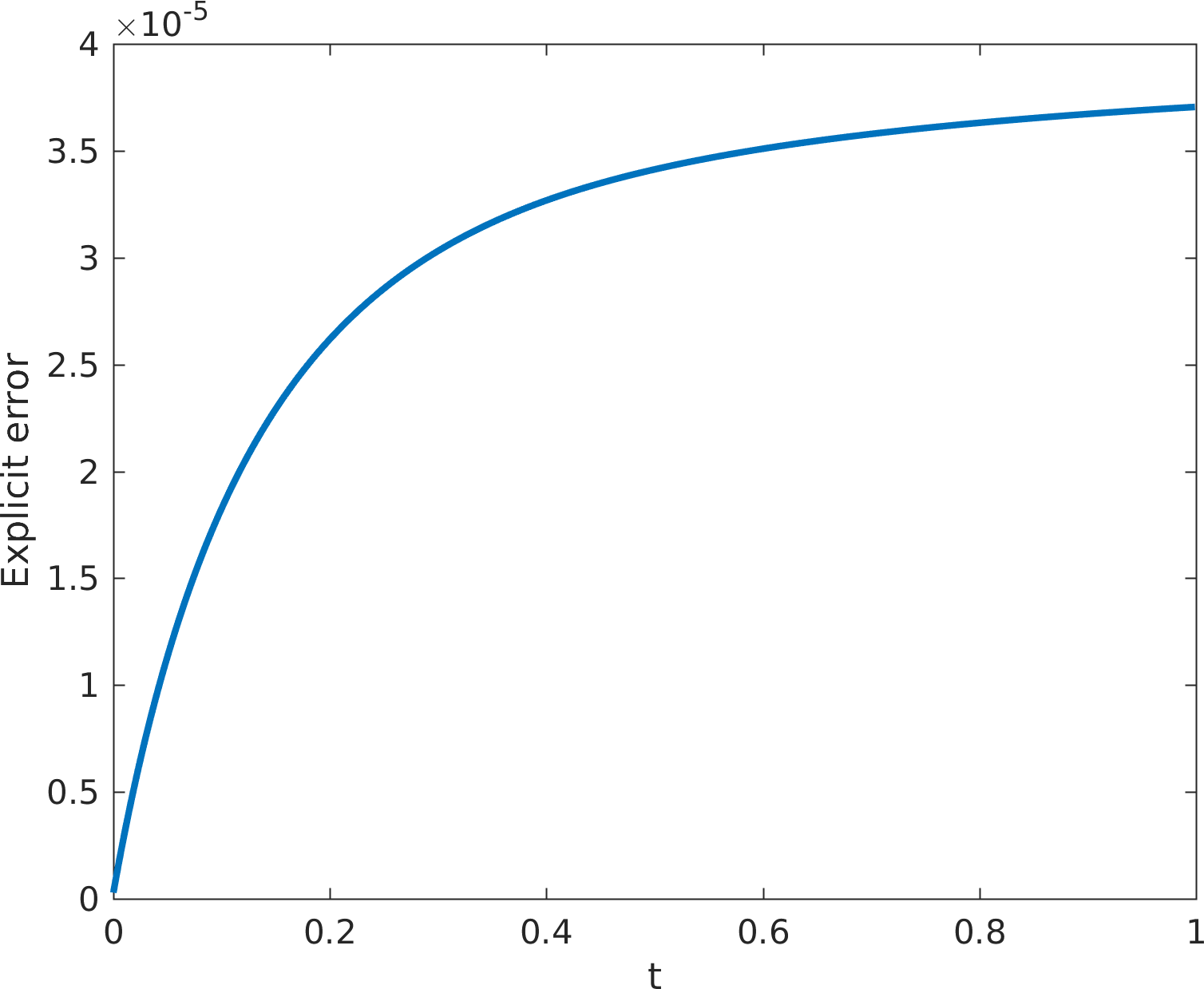
In Figure 1, we see the residual error and adjoint solution to the problem described above. We see that the initially deformed shape relaxes towards its resting configuration as a circle. We also observe some concentration in the error where the curvature is highest. In Figure 2, the time dependence of the explicit error, residual error, and adjoint solution norms are shown. The quadrature error is not shown since it behaves very similarly to the explicit error term. The error terms grow rapidly at first, followed by a period of slow growth as the boundary approaches its resting configuration. The adjoint solution remains small even at $t=0$ and gradually decays across the time interval.

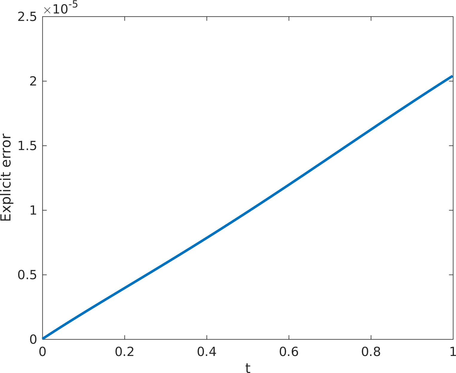
As a second example, we consider a circular boundary that is deformed in a background shear velocity field of the form $\boldsymbol{u}=\left(y,0\right)$. In Figure 3, we see the extension and rotation of a circular elastic body in response to a shear flow field. The coloring of the deforming object corresponds to the magnitude of the regularization error. Figure 4 depicts the time dependence of the $\ell_{2}$ norm over space during this deformation. We see that the adjoint solution remains small, but that given the numerical parameters of our simulation, the regularization error dominates the residual and explicit errors and increases roughly linearly in time.

In [20], the method of regularized Stokeslets was used to model a three dimensional network of fibers immersed in a fluid. This is of interest as there are number of application in biology where the fluid structure interactions of such materials are of importance. The application in [20] was geared towards understanding how a spermatocyte swims through a material known as the zona pellucida that surrounds ooctyes. Another potential application is in the study of biofilms growing in a slowly moving fluid. In this case, the particles of the method of regularized Stokeslets represent bacteria cells, and are not elements of a discretized surface. In this case, the ODE system is exact no longer an approximation of a PDE, but forms the governing equations. Regularization in this context is typically used as a means of ensuring stability of the resulting numerical simulations by limiting the velocity when bacteria approach each other. The choice of length scale then depends on the level of resolution needed in the simulation.

Following [20, 21], we write

	$\displaystyle\dot{\boldsymbol{x}}_{k}(t)$	$\displaystyle=$	$\displaystyle\sum_{j}\boldsymbol{U}_{\epsilon}(\boldsymbol{x}_{k}-\boldsymbol{x}_{j})\boldsymbol{f}_{kj}(t)m_{j}$
	$\displaystyle\boldsymbol{f}_{kj}(t)$	$\displaystyle=$	$\displaystyle\ell_{kj}^{2}E_{kj}\left(\frac{|\boldsymbol{x}_{k}(t)-\boldsymbol{x}_{j}(t)|}{\ell_{kj}}-1\right)\frac{\boldsymbol{x}_{k}(t)-\boldsymbol{x}_{j}(t)}{|\boldsymbol{x}_{k}(t)-\boldsymbol{x}_{j}(t)|}$

Note that $f_{kj}(t)=-f_{jk}(t)$. In [21, 20], the resting length is allowed to change in order to incorporate viscoelastic effects, but for simplicity, we consider only the elastic (constant resting length) case here.

As a test problem, we consider 100 points that form a network of fibers with a connectivity rule that if $|\boldsymbol{x}_{i}-\boldsymbol{x}_{j}|\leq r_{connect}$, at time 0, then $\boldsymbol{x}_{i}$ and $\boldsymbol{x}_{j}$ are attached by an elastic spring, and if $|\boldsymbol{x}_{i}-\boldsymbol{x}_{j}|>r_{connect}$, then there is no attachment. In Figure 5, an image of such a network is depicted.

As an example problem, we place the elastically connected bacteria in a linear flow field, $\boldsymbol{u}(\boldsymbol{x})=\boldsymbol{C}\cdot\boldsymbol{x}$ where $C$ is a second order tensor. The velocity of each point is then set to

$$\dot{\boldsymbol{x}}_{k}(t)=\sum_{j}\boldsymbol{U}_{\delta}(\boldsymbol{x}_{k}-\boldsymbol{x}_{j})\boldsymbol{f}_{kj}(t)m_{j}+\boldsymbol{u}(\boldsymbol{x}_{k}(t)).$$

The linear background velocity field appears in the error representation formula and adjoint equation. The ODE operator is augmented from $\boldsymbol{\mathcal{S}}_{\delta}^{h}[\boldsymbol{F}[\boldsymbol{x}],\boldsymbol{x}]$ to become

$$\boldsymbol{F}(t,\boldsymbol{x})=\boldsymbol{\mathcal{S}}_{\epsilon}^{h}[\boldsymbol{x}]+\boldsymbol{u}(\boldsymbol{x}).$$

The addition of $\boldsymbol{u}(\boldsymbol{x})$ is then carried through all of the error components Equations (8)-(10). In the adjoint equation, we obtain an additional term of the form

$$\boldsymbol{C}^{T}\cdot\boldsymbol{\phi}.$$

For a general, nonlinear velocity field, the resulting term in the linearized adjoint equation would depend on $\boldsymbol{x}$, e.g. $\boldsymbol{C}^{T}(\boldsymbol{x})\cdot\boldsymbol{\phi}$. Various choices for $\boldsymbol{C}$ lead to shear flow, straining flow, and rotational flow [18].

Alternatively, it is also possible to model situations where flow is driven by forces on the bacteria, e.g. gravitational settling of particles. In this case, the force on each particle would be of the form

$$\boldsymbol{F}[\boldsymbol{x}]+\boldsymbol{g}.$$

Since gravitational force is independent of position and time, the adjoint equation is not changed, and the error formulas are only modified through a different force relation.

Other examples of interest include cases where the forces depend on position, or when the positions of a subset of the particles is predetermined. The former case may occur with charged particles in an external field, and the latter may occur if some of the particles are assumed to be adhered to a moving boundary. Furthermore, the methods discussed here are directly applicable kernels aside from the free-space Green’s function. For instance, the techniques developed here may be applied to half-plane flows, or flows in a sphere where Green’s functions may be obtained through the method of images [18].

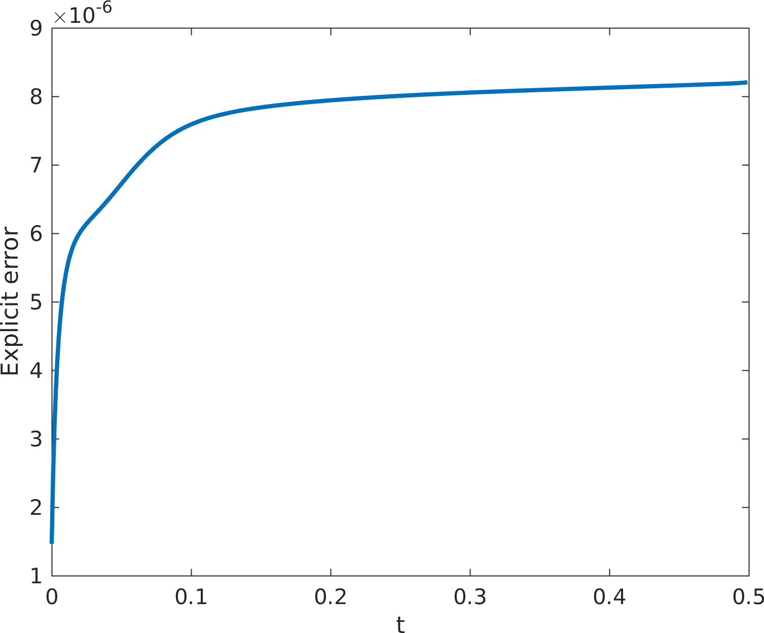
In Figure 6 the accumulation of explicit error, and the magnitude of the components of $\boldsymbol{\phi}$ are plotted versus time. We observe that the magnitude of $\boldsymbol{\phi}(t)$ grows approximately linearly over time and that the explicit error accumulation seems to grow most rapidly at the beginning of the simulation.

References

- [1] Christopher Anderson and Claude Greengard. On Vortex Methods. SIAM Journal on Numerical Analysis, 22(3):413–440, June 1985.
- [2] Vivian Aranda, Ricardo Cortez, and Lisa Fauci. A model of stokesian peristalsis and vesicle transport in a three-dimensional closed cavity. Journal of biomechanics, 48(9):1631–1638, 2015.
- [3] JC Butcher. On fifth and sixth order explicit runge-kutta methods: order conditions and order barriers. Canadian Applied Mathematics Quarterly, 17(3):433–445, 2009.
- [4] Yang Cao and Linda Petzold. A Posteriori Error Estimation and Global Error Control for Ordinary Differential Equations by the Adjoint Method. SIAM Journal on Scientific Computing, 26(2):359–374, January 2004.
- [5] J. B. Collins, D. Estep, and S. Tavener. A posteriori error analysis for finite element methods with projection operators as applied to explicit time integration techniques. BIT Numerical Mathematics, 55(4):1017–1042, December 2015.
- [6] Ricardo Cortez. On the Accuracy of Impulse Methods for Fluid Flow. SIAM Journal on Scientific Computing, 19(4):1290–1302, July 1998.
- [7] Ricardo Cortez. The Method of Regularized Stokeslets. SIAM Journal on Scientific Computing, 23(4):1204–1225, January 2001.
- [8] Ricardo Cortez, Lisa Fauci, and Alexei Medovikov. The method of regularized Stokeslets in three dimensions: Analysis, validation, and application to helical swimming. Physics of Fluids, 17(3):031504, March 2005.
- [9] Donald Estep. A Posteriori Error Bounds and Global Error Control for Approximation of Ordinary Differential Equations. SIAM Journal on Numerical Analysis, 32(1):1–48, February 1995.
- [10] Jason F. Hammond, Elizabeth J. Stewart, John G. Younger, Michael J. Solomon, and David M. Bortz. Variable Viscosity and Density Biofilm Simulations using an Immersed Boundary Method, Part I: Numerical Scheme and Convergence Results. CMES, 98(3):295–340, 2014.
- [11] Sangtae Kim and Seppo J. Karrila. Microhydrodynamics: principles and selected applications. Butterworth-Heinemann series in chemical engineering. Butterworth-Heinemann, Boston, 1991.
- [12] Dirk P Kroese and Zdravko I Botev. Spatial process generation. arXiv preprint arXiv:1308.0399, 2013.
- [13] Gerasimos E Ladas and Vangipuram Lakshmikantham. Differential equations in abstract spaces. Elsevier, 1972.
- [14] Olga A Ladyzhenskaya. The mathematical theory of viscous incompressible flow, volume 12. Gordon & Breach New York, 1969.
- [15] Fanghua Lin and Jiajun Tong. Solvability of the Stokes Immersed Boundary Problem in Two Dimensions. arXiv, 1703.03124, 2017.
- [16] Andrew Majda and Andrea L. Bertozzi. Vorticity and incompressible flow. Cambridge texts in applied mathematics. Cambridge University Press, Cambridge ; New York, 2002.
- [17] Y. Mori, Analise Rodenberg, and Daniel Spirn. Well-posedness and global behavior of the Peskin problem of an immersed elastic filament in Stokes flow. arXiv, 1704.08392, 2017.
- [18] Constantine Pozrikidis. Boundary integral and singularity methods for linearized viscous flow. Cambridge University Press, 1992.
- [19] Jay A. Stotsky, Jason F. Hammond, Leonid Pavlovsky, Elizabeth J. Stewart, John G. Younger, Michael J. Solomon, and David M. Bortz. Variable viscosity and density biofilm simulations using an immersed boundary method, part II: Experimental validation and the heterogeneous rheology-IBM. Journal of Computational Physics, 317:204–222, July 2016.
- [20] Jacek K. Wrobel, Ricardo Cortez, and Lisa Fauci. Modeling viscoelastic networks in Stokes flow. Physics of Fluids, 26(11):113102, November 2014.
- [21] Jacek K. Wrobel, Sabrina Lynch, Aaron Barrett, Lisa Fauci, and Ricardo Cortez. Enhanced flagellar swimming through a compliant viscoelastic network in Stokes flow. Journal of Fluid Mechanics, 792:775–797, April 2016.