Magnetic quenching of the inverse cascade in rapidly rotating convective turbulence

The subsurface regions of stars and the fluid cores of planets are typically characterized by rapid rotation, buoyancy-driven convective turbulence, and electromagnetic fields generated by the dynamo mechanism that converts the kinetic energy of fluid motion into electromagnetic energy. The dynamical state of such systems is characterized by several non-dimensional parameters, including the Reynolds number, $Re_{H}=UH/\nu$, the Ekman number, $E_{H}=\nu/(2\Omega H^{2})$, and the Rossby number, $Ro_{H}=U/(2\Omega H)$. Here $U$ and $H$ represent a typical speed and length-scale of the flow, $\nu$ is the kinematic viscosity and $\Omega$ is the rotation rate. The Reynolds, Ekman and Rossby numbers represent the relative sizes of inertia to viscous forces, viscous forces to the Coriolis force, and inertia to the Coriolis force, respectively. Rapidly rotating turbulent flows are characterized by $Re_{H}\gg 1$ and $E_{H}\ll Ro_{H}\ll 1$. An important physical property of electrically conducting fluids is the magnetic Prandtl number, $Pm=\nu/\eta$, where $\eta$ is the magnetic diffusivity. For the Earth’s liquid outer core these parameters are estimated to be $Re_{H}\approx 10^{8}$, $E_{H}\approx 10^{-15}$, $Ro_{H}\approx 10^{-7}$ and $Pm\approx 10^{-6}$ Olson (2015). In contrast, the most extreme direct numerical simulation (DNS) spherical dynamo study to date Schaeffer et al. (2017) used values of $E_{H}=5\times 10^{-8}$ and $Pm=10^{-1}$, and reached $Re_{H}\approx 5\times 10^{3}$. Although of crucial importance for understanding magnetohydrodynamics (MHD), it is unknown how the results of such DNS studies extrapolate to natural systems. For flows with sufficiently large values of $Re_{H}$, and subject to a broad variety of forcing mechanisms, rapidly rotating three-dimensional turbulence gives rise to the formation of motions with large lateral scales relative to the forcing scale Smith and Waleffe (1999); Favier et al. (2014); Rubio et al. (2014); Guervilly et al. (2014); Le Reun et al. (2017). Such flows result from an inverse energy cascade that leads to a net transfer of kinetic energy from the small-scale motions to large-scale motions of the flow. For hydrodynamic, non-magnetic turbulence, the ultimate scale at which the inverse cascade ceases is dependent upon the geometry. In a Cartesian geometry with equal horizontal dimensions, the cascade leads to domain-filling large-scale vortices (LSVs) Guervilly et al. (2015); Le Reun et al. (2017); Rubio et al. (2014). In a spherical geometry, the inverse cascade is halted at the so-called Rhines scale Rhines (1975). The Rhines scale represents a dynamical cross-over between eddy dynamics that dominate on small-scales and Rossby wave dynamics that dominate on large-scales; it is thought to control the latitudinal extent of alternating winds in the outer, electrically-insulating fluid regions of giant planet atmospheres Cabanes et al. (2017).

It has been suggested, based on the results of DNS studies Guervilly et al. (2015); Lin et al. (2016); Guervilly et al. (2017), that inverse-cascade-generated LSVs might be important for generating large-scale (i.e. domain-scale) magnetic fields in planets and stars. However, rapid rotation alone is sufficient for generating large-scale magnetic fields Calkins et al. (2015), even for laminar, small-Reynolds-number flows that lack an inverse cascade Soward (1974); Calkins et al. (2016a); Calkins et al. (2016b). In the asymptotic limit of rapid rotation, LSVs are unimportant for the onset of dynamo action Calkins et al. (2016b). However, the influence of magnetic field on the inverse cascade remains poorly understood due, in large part, to the limited parameter range of previous DNS studies. It is evident that the Rossby number, in particular, is not low enough in many DNS investigations to be applicable to planetary systems; this effect is evident in DNS studies in which LSVs shows a preference for cyclonic circulation (i.e. in the same direction as the system rotation vector) Guervilly et al. (2015); Favier et al. (2014). For sufficiently small Rossby numbers the LSV consists of a dipolar vortex with no preference for a particular circulation direction Stellmach et al. (2014). Thus, lower Rossby number simulations are necessary to better understand the planetary regime.

It should be noted that rapid rotation is not a requirement for the inverse cascade. Previous work has shown that imposed magnetic fields can also lead to an inverse energy cascade Hossain (1991); Alexakis (2011); Reddy and Verma (2014). In addition, studies of two-dimensional turbulence have shown that sufficiently strong magnetic fields (Tobias et al., 2007) and Lorentz-force-like forcing terms (Seshasayanan et al., 2014) can disrupt the inverse cascade. Here we find that a similar effect occurs in rapidly rotating, convection-driven turbulence, which represents a system that is more applicable to the study of planets and stars.

Although previous work has suggested that the presence of magnetic fields can prevent the formation of large-scale structures in rapidly rotating convective systems (Guervilly et al., 2017), no systematic study has been performed to date that fully elucidates the physical mechanism by which a magnetic field influences the inverse cascade. In this regard, we explore the problem by utilizing an asymptotically reduced form of the governing equations of MHD Calkins et al. (2015), that is valid in the geo- and astrophysically relevant limits of $(E_{H},Ro_{H},Pm)\rightarrow 0$ with $Re_{H}\gg 1$. We consider rotating Rayleigh-Bénard convection in a horizontally-periodic plane layer of incompressible fluid of depth $H$, with constant vertical gravity and rotation vectors ($\textbf{g}=-g\textbf{e}_{z}$ and $\mathbf{\Omega}=\Omega\textbf{e}_{z}$, respectively, where $\textbf{e}_{z}$ is the vertical unit vector). A constant temperature difference $\Delta\theta$ between the top and bottom boundaries is maintained to drive convective motions. Here we provide only a brief overview of the derivation of the model. Further details can be found in previous work (Sprague et al., 2006; Calkins et al., 2015; Calkins et al., 2016a; Calkins et al., 2016b; Plumley et al., 2018). We assume that the small convective spatial scale $l$ and the Rayleigh number $Ra_{H}=g\alpha\Delta\theta H^{3}/(\kappa\nu)$ ($\alpha$ is the thermal expansion coefficient and $\kappa$ is the thermal diffusivity) scale, respectively, as $E_{H}^{1/3}H$ and $E_{H}^{-4/3}$, as informed from linear theory Chandrasekhar (1961). These scalings ensure scale separation between $l$ and the depth of the layer such that $\epsilon\equiv l/H=E_{H}^{1/3}\ll 1$, which translates into separation between the small-scale coordinate system $(x,y,z)$ and the domain-scale, vertical coordinate $Z=\epsilon z$. The equations are separated into mean (averaged over the small horizontal scales) and fluctuating components. We then expand each dependent variable ($f$, say) in a power series of the form $f=f_{0}+\epsilon^{1/2}f_{1/2}+\epsilon f_{1}+\ldots$, take the limit $\epsilon\rightarrow 0$, and collect terms of equal magnitude in the resulting system of equations. Upon integrating on the small vertical coordinate $z$, we obtain the following system for the asymptotically reduced equations (where the ordering subscripts on the variables have been dropped):

The overbar denotes an average over fast spatiotemporal scales, and we use the notation $D^{\perp}_{t}={\partial_{t}}+\mathbf{u}_{\perp}\cdot\nabla_{\perp}$ and $\nabla_{\perp}=(\partial_{x},\partial_{y})$. The geostrophic streamfunction (pressure) is denoted by $\psi$ and defined by $\mathbf{u}_{\perp}=-\nabla_{\perp}\times(\psi\textbf{e}_{z})$; $\zeta={\nabla_{\perp}^{2}}\psi$ is the axial vorticity and $w$ is the vertical velocity; $\vartheta$ and $\overline{\Theta}$ are the fluctuating and horizontally averaged temperature; $\overline{\bf B}$, $b_{z}$ and $j_{z}=\textbf{e}_{z}\cdot\nabla_{\perp}\times\mathbf{b}$ are the mean magnetic field, fluctuating vertical magnetic field and vertical current density, respectively; $\widetilde{Ra}$ and $\widetilde{Q}$ are, respectively, the asymptotically reduced Rayleigh and Chandrasekhar numbers (see below). For the above set of equations, time has been scaled by the small-scale (horizontal) viscous diffusion timescale $l^{2}/\nu$, the magnetic field has been scaled by the magnitude of the mean magnetic field $\mathcal{B}$, and temperature has been scaled by $\Delta\theta$. We impose a mean, horizontal magnetic field defined by

that satisfies perfectly conducting electromagnetic boundary conditions. Mean magnetic fields of similar spatial structure are found to be generated by dynamo action near the onset of rotating Rayleigh-Bénard convection Soward (1974); Stellmach and Hansen (2004); Calkins et al. (2016b); Guervilly et al. (2017). Even for strongly forced convection, the mean field appears to retain a spiralling structure Calkins et al. (2016b); Guervilly et al. (2017). The use of an imposed, rather than self-generated, magnetic field allows for precise control of the field magnitude. We also utilize the quasi-static MHD approximation on the small convective scale, valid for the small values of $Pm$ typical of planetary and stellar interiors. The dynamics are controlled by three non-dimensional parameters: the asymptotically-scaled Chandrasekhar number, $\widetilde{Q}=Q_{H}E_{H}^{2/3}$ (where $Q_{H}=\mathcal{B}^{2}H^{2}/(\mu_{0}\rho\nu\eta)$ and $\mu_{0}$ is the magnetic permeability of free space); the asymptotically-scaled Rayleigh number, $\widetilde{Ra}=Ra_{H}E_{H}^{4/3}$; and the thermal Prandtl number, $Pr=\nu/\kappa$. Here $(\widetilde{Ra},\widetilde{Q})=O(1)$ (or, more specifically, $\widetilde{Ra},\widetilde{Q}<\epsilon^{-1/2}$ so that buoyancy and the Lorentz force do not enter lower orders of the asymptotic expansion) and we use $Pr=1$ in order to allow for comparison with previous studies. For the Earth’s outer core, $E_{H}=O(10^{-15})$, and the asymptotic model captures dynamically relevant values of $Ra_{H}=O(10^{20})$ and $Q_{H}=O(10^{10})$. The boundary conditions for (1)-(6) are impenetrable, stress-free, fixed-temperature and perfectly electrically conducting. The equations are discretized in the horizontal and vertical dimensions with Fourier series and Chebyshev polynomials, respectively. The horizontal size of the domain of integration is set to 10 times the critical wavelength at the onset of convection in both the $x$ and $y$ directions. The time-stepping is performed with a third order Runge-Kutta scheme Spalart et al. (1991). Simulations of the hydrodynamical version ($\widetilde{Q}=0$) of (1)-(6) have shown excellent quantitative agreement with laboratory experiments and DNS Stellmach et al. (2014); Plumley et al. (2016).

Numerical simulations were performed over a broad range of $\widetilde{Q}$ and $\widetilde{Ra}$ (see Supplemental Material at [URL will be inserted by the publisher] for details of the numerical simulations performed in this study), allowing for the investigation of flow regimes ranging from laminar magnetoconvection, up through rapidly rotating magnetoconvective turbulence. For $\widetilde{Q}=0$, $\widetilde{Ra}\geq 40$ generates sufficiently turbulent flows that result in the formation of an LSV Rubio et al. (2014). The left panel of Figure 1 show instantaneous snapshots of the volume-rendered geostrophic streamfunction (pressure) and vertically integrated axial vorticity for $\widetilde{Q}=0,\widetilde{Ra}=160$. In the rapidly rotating limit considered here, the LSV is dipolar in structure and fills the horizontal extent of the domain such that the (energetically) dominant horizontal wavenumber is the box scale, $k=1$, where $k$ is the modulus of the horizontal wavenumber k. In agreement with previous studies Julien et al. (2012); Rubio et al. (2014); Guervilly et al. (2014), the baroclinic, convective dynamics is not significantly affected by the presence of the LSV. The central and right panels of Figure 1 show the corresponding cases with non-dimensional magnetic field strengths of $\widetilde{Q}=1$ and $\widetilde{Q}=2$, respectively, for $\widetilde{Ra}=160$. It is evident that stronger magnetic fields yield a significant reduction in the strength of the horizontal box-scale mode of the depth-averaged motion, to the point that it is no longer visible.

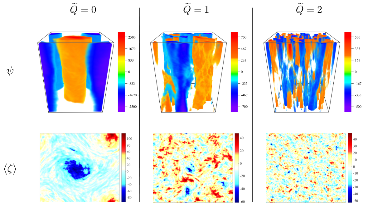
The formation of the LSV is due to transfer of energy from the convective length-scale (where energy is injected) to the largest scales allowed in the system. This process is described by the spectral evolution equation for the barotropic (vertically integrated, horizontal) kinetic energy $K_{bt}(k)$,

The four terms on the right-hand side are: (1) the transfer of energy between barotropic modes of wavenumber k,

where $\left<\psi\right>_{\textbf{k}}$ is the horizontal Fourier transform of the vertically averaged streamfunction $\left<\psi\right>$, the superscript $*$ denotes a complex conjugate, $\mathcal{F}_{\textbf{k}}[\cdot]$ indicates the horizontal Fourier transform of the argument in square brackets, $J[\cdot]$ is the Jacobian differential operator acting on the arguments in square brackets, the symbol $\circ$ indicates a Hadamard (element-wise) product (both $\left<\psi\right>_{\textbf{k}}$ and $\mathcal{F}_{\textbf{k}}\left[J[\left<\psi\right>,\left<\zeta\right>]\right]$ are two-dimensional matrices), $\textrm{Re}\left\{\cdot\right\}$ is the real part of the argument in curly brackets and the sum is taken over all horizontal wavenumbers; (2) the transfer of energy between the barotropic and baroclinic (convective) modes

(3) the transfer of energy to the barotropic mode from the baroclinic magnetic field

and (4) the viscous dissipation of the barotropic mode

With the above definitions, positive (negative) values of $T_{k}$ and $F_{k}$ indicate energy is being transferred to (from) the barotropic mode $k$ from the interaction of all the other modes. Both $L_{k}$ and $D_{k}$ are negative-definite.

Calculating each of the above functions allows for quantifying the transfer of energy across different spatial scales; the results are shown in Figure 2 for $\widetilde{Ra}=160$.

In the $\widetilde{Q}=0$ case, as previously documented Rubio et al. (2014), there is a net transfer of energy to the largest scales of the barotropic mode due mostly to the non-linear interaction with the baroclinic dynamics ($F_{k}$), and partly to the interaction between different components of the barotropic flow ($T_{k}$). Since the sum of these two terms is greater than the dissipation $D_{k}$, there is a net growth of barotropic kinetic energy at large-scales, leading to the formation of the LSV. For large-scale flows, viscous friction can only become important when the flow speeds become large. Because of this, the formation of the LSV leads to a slow growth of the barotropic kinetic energy with time (see Supplemental Material at [URL will be inserted by the publisher] for time series of the kinetic energy for $\widetilde{Ra}=40$ and $\widetilde{Ra}=160$ cases and different values of $\widetilde{Q}$). For $\widetilde{Q}=0.1$ the presence of the magnetic field allows for the transfer of energy between baroclinic magnetic energy and barotropic kinetic energy (via $L_{k}$), which contributes to the dissipation of energy at large-scales. Indeed, $\widetilde{Q}\left<\overline{\textbf{B}}\cdot\nabla j^{\prime}_{z}\right>=-\widetilde{Q}\left<\sum_{\textbf{k}}k^{-2}|\overline{\textbf{B}}\cdot\textbf{k}|^{2}\left<\zeta\right>_{\textbf{k}}\right>$ acts as a dissipative term, proportional to the barotropic component of $\zeta_{\textbf{k}}$. Since $F_{k}$ is still dominant at larger scales, there is a net growth of barotropic kinetic energy and LSV formation. The net positive transfer of energy in these cases is due to the temporal averages being calculated over a time-span over which the inverse cascade has not been completely saturated. With time, the dissipation (both viscous and ohmic) grows in magnitude and eventually balances the baroclinic-to-barotropic and the barotropic-to-barotropic transfers, but the dominant wavenumber remains $k=1$. As $\widetilde{Q}$ is increased we find that an inverse cascade (towards scales larger than the injection scale $k=10$) is still present. However, $F_{k}$ and $T_{k}$ no longer transport energy to the largest scales (notice the kinetic energy peak at $k=5$ for $\widetilde{Q}=2$ in Figure 2), and the ohmic dissipation ($L_{k}$) increases in magnitude to counterbalance $F_{k}$ and $T_{k}$. LSVs do not form in such cases, leading to a rapid saturation of the kinetic energy.

In Figure 3 we show the barotropic kinetic energy spectra for the $\widetilde{Ra}=160$ case. The formation of an LSV for $\widetilde{Q}=0$ and $\widetilde{Q}=0.1$ is evident by the dominance of the box-scale mode. For $\widetilde{Q}=1$ and $\widetilde{Q}=2$ the inverse cascade causes local maxima to be present at $k=2$ and $k=5$, respectively. The $k^{-3}$ slope shown in the plot is expected in the inertial subrange, which is consistent with forward enstrophy cascade Kraichnan (1967), and at the largest scale in presence of large-scale condensates Smith and Waleffe (1999); Rubio et al. (2014). The $k=-5/3$ line is added for reference.

For the values of $\widetilde{Ra}$ and $\widetilde{Q}$ considered here, Figure 4(a) shows that the presence of magnetic field does not have an appreciable influence on the convective (vertical) flow speeds, as characterized by the rms small-scale Reynolds number, $\widetilde{Re}$. For $\widetilde{Ra}=160$ the relative difference in $\widetilde{Re}$ is less than $30\%$ between the $\widetilde{Q}=0$ and $\widetilde{Q}=2$ cases. The threshold for LSV formation for $\widetilde{Q}=0$ is $\widetilde{Re}\gtrsim 10$; all of the magnetic cases with $\widetilde{Ra}\gtrsim 40$ satisfy this hydrodynamic criteria, showing that $\widetilde{Re}$ alone is insufficient for determining when an LSV forms. To better characterize the conditions that favor LSV formation in the presence of magnetic field, we calculate the reduced magnetic interaction parameter $\widetilde{N}$ Cioni et al. (2000)

where $\mathbf{b}$ and $\mathbf{u}$ are the small-scale magnetic and velocity fields, respectively. The interaction parameter is a measure of the relative magnitudes of the Lorentz force and non-linear advection. Figure 4(b) shows that the formation of an LSV is possible for $\widetilde{N}\lesssim 0.013$. Above this threshold the magnetic field plays a significant role in the dynamics, despite the large $\widetilde{Re}$. The exact threshold value likely depends on the geometry of the mean-field.

Our results suggest that it is possible to determine whether LSVs form in natural settings, based on properties that are either directly observable, or inferred from measurements, laboratory experiments and numerical simulations. For instance, ab-initio calculations can be used to constrain the radial variation of density, viscosity and electrical conductivity within Jupiter French et al. (2012). Magnetic field models of Jupiter, as obtained from the recent Juno spacecraft observations Connerney et al. (2018), help to estimate $\widetilde{Q}$ in the outermost layers of the planet, where electrical conductivity is small. To estimate $\widetilde{Re}$ we use zonal-mean meridional velocities derived from Cassini spacecraft observations Galperin et al. (2014), which most likely constitute a lower bound on the convective velocities, and assume they do not change significantly with depth. Together, this data suggests that $\widetilde{N}\geq 0.013$ for $r\lesssim 0.87R_{J}$, where $r$ is the distance from the center of Jupiter and $R_{J}$ is the equatorial radius (see Figure 5). This depth agrees with the location of the dynamo region’s upper limit estimated from ab-initio calculations French et al. (2012), from numerical simulation results Duarte et al. (2013) and from the depth of zonal flows based on Juno’s gravitational field observations Kong et al. (2018) (although it is somewhat deeper than the estimated depth reached by deep zonal jets Kaspi et al. (2018); Guillot et al. (2018); Kong et al. (2018)), suggesting that the observed large-scale vortices Adriani et al. (2018) and winds do not penetrate into the dynamo region of Jupiter. For the Earth’s outer core we estimate $\widetilde{Re}=10^{3}$ and $\widetilde{Q}\approx 3\times 10^{5}$ for accepted values of core flow speed and viscosity Jones (2015) and a magnetic field intensity of $3$ mT Gillet et al. (2010). These two values give $\widetilde{N}\approx 300$, which is well above the threshold of $\widetilde{N}\approx 0.013$ identified from Figure 4(b). We conclude that, at the present time, convectively-generated LSVs are likely not present in the Earth’s core.

References

- Olson (2015) P Olson, “Core dynamics: an introduction and overview,” Treatise on Geophysics , 1–25 (2015).
- Schaeffer et al. (2017) N. Schaeffer, D. Jault, H.-C. Nataf, and A. Fournier, “Turbulent geodynamo simulations: a leap towards Earth’s core,” Geophysical Journal International 211, 1–29 (2017).
- Smith and Waleffe (1999) Leslie M Smith and Fabian Waleffe, “Transfer of energy to two-dimensional large scales in forced, rotating three-dimensional turbulence,” Physics of fluids 11, 1608–1622 (1999).
- Favier et al. (2014) Benjamin Favier, L J Silvers, and M R E Proctor, “Inverse cascade and symmetry breaking in rapidly rotating Boussinesq convection,” Physics of Fluids 26, 096605 (2014).
- Rubio et al. (2014) Antonio M Rubio, Keith Julien, Edgar Knobloch, and Jeffrey B Weiss, “Upscale energy transfer in three-dimensional rapidly rotating turbulent convection,” Physical Review Letters 112, 144501 (2014).
- Guervilly et al. (2014) Céline Guervilly, David W Hughes, and Chris A Jones, “Large-scale vortices in rapidly rotating Rayleigh–Bénard convection,” Journal of Fluid Mechanics 758, 407–435 (2014).
- Le Reun et al. (2017) Thomas Le Reun, Benjamin Favier, Adrian J Barker, and Michael Le Bars, “Inertial wave turbulence driven by elliptical instability,” Physical Review Letters 119, 034502 (2017).
- Guervilly et al. (2015) Céline Guervilly, David W Hughes, and Chris A Jones, “Generation of magnetic fields by large-scale vortices in rotating convection,” Physical Review E 91, 041001 (2015).
- Rhines (1975) Peter B Rhines, “Waves and turbulence on a beta-plane,” Journal of Fluid Mechanics 69, 417–443 (1975).
- Cabanes et al. (2017) Simon Cabanes, Jonathan Aurnou, Benjamin Favier, and Michael Le Bars, “A laboratory model for deep-seated jets on the gas giants,” Nature Physics 13, 387 (2017).
- Lin et al. (2016) Yufeng Lin, Philippe Marti, Jerome Noir, and Andrew Jackson, “Precession-driven dynamos in a full sphere and the role of large scale cyclonic vortices,” Physics of Fluids 28, 066601 (2016).
- Guervilly et al. (2017) Céline Guervilly, David W Hughes, and Chris A Jones, “Large-scale-vortex dynamos in planar rotating convection,” Journal of Fluid Mechanics 815, 333–360 (2017).
- Calkins et al. (2015) Michael A. Calkins, Keith Julien, Steven M. Tobias, and Jonathan M. Aurnou, “A multiscale dynamo model driven by quasi-geostrophic convection,” Journal of Fluid Mechanics 780, 143–166 (2015).
- Soward (1974) A. M. Soward, “A convection-driven dynamo: I. the weak field case,” Philosophical Transactions of the Royal Society A 275, 611–646 (1974).
- Calkins et al. (2016a) M. A. Calkins, K. Julien, S. M. Tobias, J. M. Aurnou, and P. Marti, “Convection-driven kinematic dynamos at low Rossby and magnetic Prandtl numbers: single mode solutions,” Phys. Rev. E. 93, 023115 (2016a).
- Calkins et al. (2016b) M. A. Calkins, L. Long, D. Nieves, K. Julien, and S. M. Tobias, “Convection-driven kinematic dynamos at low Rossby and magnetic Prandtl numbers,” Physical Review Fluids 1, 083701 (2016b).
- Stellmach et al. (2014) S Stellmach, M Lischper, K Julien, G Vasil, J S Cheng, A Ribeiro, E M King, and J M Aurnou, “Approaching the asymptotic regime of rapidly rotating convection: boundary layers versus interior dynamics,” Physical Review Letters 113, 254501 (2014).
- Hossain (1991) Murshed Hossain, “Inverse energy cascades in three-dimensional turbulence,” Physics of Fluids B: Plasma Physics 3, 511–514 (1991).
- Alexakis (2011) Alexandros Alexakis, “Two-dimensional behavior of three-dimensional magnetohydrodynamic flow with a strong guiding field,” Physical Review E 84, 056330 (2011).
- Reddy and Verma (2014) K Sandeep Reddy and Mahendra K Verma, “Strong anisotropy in quasi-static magnetohydrodynamic turbulence for high interaction parameters,” Physics of Fluids 26, 025109 (2014).
- Tobias et al. (2007) Steven M Tobias, Patrick H Diamond, and David W Hughes, “-plane magnetohydrodynamic turbulence in the solar tachocline,” The Astrophysical Journal Letters 667, L113 (2007).
- Seshasayanan et al. (2014) Kannabiran Seshasayanan, Santiago Jose Benavides, and Alexandros Alexakis, “On the edge of an inverse cascade,” Physical Review E 90, 051003 (2014).
- Sprague et al. (2006) Michael Sprague, Keith Julien, Edgar Knobloch, and Joseph Werne, “Numerical simulation of an asymptotically reduced system for rotationally constrained convection,” Journal of Fluid Mechanics 551, 141–174 (2006).
- Plumley et al. (2018) Meredith Plumley, Michael A Calkins, Keith Julien, and Steven M Tobias, “Self-consistent single mode investigations of the quasi-geostrophic convection-driven dynamo model,” Journal of Plasma Physics 84 (2018).
- Chandrasekhar (1961) Subrahmanyan Chandrasekhar, Hydrodynamic and Hydromagnetic stability (Courier Corporation, 1961).
- Stellmach and Hansen (2004) Stephan Stellmach and Ulrich Hansen, “Cartesian convection driven dynamos at low Ekman number,” Physical Review E 70, 056312 (2004).
- Spalart et al. (1991) Philippe R Spalart, Robert D Moser, and Michael M Rogers, “Spectral methods for the navier-stokes equations with one infinite and two periodic directions,” Journal of Computational Physics 96, 297–324 (1991).
- Plumley et al. (2016) Meredith Plumley, Keith Julien, Philippe Marti, and Stephan Stellmach, “The effects of Ekman pumping on quasi-geostrophic Rayleigh–Bénard convection,” Journal of Fluid Mechanics 803, 51–71 (2016).
- Julien et al. (2012) K Julien, A M Rubio, I Grooms, and E Knobloch, “Statistical and physical balances in low Rossby number Rayleigh–Bénard convection,” Geophysical & Astrophysical Fluid Dynamics 106, 392–428 (2012).
- Kraichnan (1967) Robert H Kraichnan, “Inertial ranges in two-dimensional turbulence,” The Physics of Fluids 10, 1417–1423 (1967).
- Cioni et al. (2000) S Cioni, S Chaumat, and J Sommeria, “Effect of a vertical magnetic field on turbulent Rayleigh-Bénard convection,” Physical Review E 62, R4520 (2000).
- Connerney et al. (2018) J E P Connerney, S Kotsiaros, R J Oliversen, J R Espley, John Leif Joergensen, P S Joergensen, José M G Merayo, Matija Herceg, J Bloxham, K M Moore, et al., “A new model of Jupiter’s magnetic field from Juno’s first nine orbits,” Geophysical Research Letters 45, 2590–2596 (2018).
- French et al. (2012) Martin French, Andreas Becker, Winfried Lorenzen, Nadine Nettelmann, Mandy Bethkenhagen, Johannes Wicht, and Ronald Redmer, “Ab initio simulations for material properties along the Jupiter adiabat,” The Astrophysical Journal Supplement Series 202, 5 (2012).
- Galperin et al. (2014) Boris Galperin, Roland MB Young, Semion Sukoriansky, Nadejda Dikovskaya, Peter L Read, Andrew J Lancaster, and David Armstrong, “Cassini observations reveal a regime of zonostrophic macroturbulence on Jupiter,” Icarus 229, 295–320 (2014).
- Duarte et al. (2013) Lúcia DV Duarte, Thomas Gastine, and Johannes Wicht, “Anelastic dynamo models with variable electrical conductivity: An application to gas giants,” Physics of the Earth and Planetary Interiors 222, 22–34 (2013).
- Kong et al. (2018) Dali Kong, Keke Zhang, Gerald Schubert, and John D Anderson, “Origin of Jupiter’s cloud-level zonal winds remains a puzzle even after Juno,” Proceedings of the National Academy of Sciences 115, 8499–8504 (2018).
- Kaspi et al. (2018) Y Kaspi, E Galanti, W B Hubbard, D J Stevenson, S J Bolton, L Iess, T Guillot, J Bloxham, J E P Connerney, H Cao, et al., “Jupiter’s atmospheric jet streams extend thousands of kilometres deep,” Nature 555, 223 (2018).
- Guillot et al. (2018) Tristan Guillot, Y Miguel, B Militzer, W B Hubbard, Y Kaspi, E Galanti, H Cao, R Helled, S M Wahl, L Iess, et al., “A suppression of differential rotation in Jupiter’s deep interior,” Nature 555, 227 (2018).
- Adriani et al. (2018) Alberto Adriani, A Mura, G Orton, C Hansen, F Altieri, M. L. Moriconi, J Rogers, G Eichstädt, T Momary, A P Ingersoll, et al., “Clusters of cyclones encircling Jupiter’s poles,” Nature 555, 216 (2018).
- Jones (2015) Chris A Jones, “Thermal and compositional convection in the outer core,” Treatise on Geophysics , 115–159 (2015).
- Gillet et al. (2010) Nicolas Gillet, Dominique Jault, Elisabeth Canet, and Alexandre Fournier, “Fast torsional waves and strong magnetic field within the Earth’s core,” Nature 465, 74–77 (2010).