Towards Better UD Parsing: Deep Contextualized Word Embeddings, Ensemble, and Treebank Concatenation
Abstract
This paper describes our system (HIT-SCIR) submitted to the CoNLL 2018 shared task on Multilingual Parsing from Raw Text to Universal Dependencies. We base our submission on Stanford’s winning system for the CoNLL 2017 shared task and make two effective extensions: 1) incorporating deep contextualized word embeddings into both the part of speech tagger and dependency parser; 2) ensembling parsers trained with different initialization. We also explore different ways of concatenating treebanks for further improvements. Experimental results on the development data show the effectiveness of our methods. In the final evaluation, our system was ranked first according to LAS (75.84%) and outperformed the other systems by a large margin.
1 Introduction
In this paper, we describe our system (HIT-SCIR) submitted to CoNLL 2018 shared task on Multilingual Parsing from Raw Text to Universal Dependencies Zeman et al. (2018). We base our system on Stanford’s winning system (Dozat et al., 2017, §2) for the CoNLL 2017 shared task Zeman et al. (2017).
Dozat and Manning (2016) and its extension Dozat et al. (2017) have shown very competitive performance in both the shared task Dozat et al. (2017) and previous parsing works Ma and Hovy (2017); Shi et al. (2017a); Liu et al. (2018b); Ma et al. (2018). A natural question that arises is how can we further improve their part of speech (POS) tagger and dependency parser via a simple yet effective technique. In our system, we make two noteworthy extensions to their tagger and parser:
- •
Incorporating the deep contextualized word embeddings (Peters et al., 2018, ELMo: Embeddings from Language Models) into the word representaton (§3);
- •
Ensembling parsers trained with different initialization (§4).
For some languages in the shared task, multiple treebanks of different domains are provided. Treebanks which are of the same language families are provided as well. Letting these treebanks help each other has been shown an effective way to improve parsing performance in both the cross-lingual-cross-domain parsing community and last year’s shared tasks Ammar et al. (2016); Guo et al. (2015); Che et al. (2017); Shi et al. (2017b); Björkelund et al. (2017). In our system, we apply the simple concatenation to the treebanks that are potentially helpful to each other and explore different ways of concatenation to improve the parser’s performance (§5).
In dealing with the small treebanks and treebanks from low-resource languages (§6), we adopt the word embedding transfer idea in the cross-lingual dependency parsing Guo et al. (2015) and use the bilingual word vectors transformation technique Smith et al. (2017)11 1 https://github.com/Babylonpartners/fastText_multilingual to map fasttext22 2 https://github.com/facebookresearch/fastText word embeddings Bojanowski et al. (2016) of the source rich-resource language and target low-resource language into the same space. The transferred parser trained on the source language is used for the target low-resource language.
We conduct experiments on the development data to study the effects of ELMo, parser ensemble, and treebank concatenation. Experimental results show that these techniques substantially improve the parsing performance. Using these techniques, our system achieved an averaged LAS of 75.84 on the official test set and was ranked the first according to LAS Zeman et al. (2018). This result significantly outperforms the others by a large margin.33 3 http://universaldependencies.org/conll18/results.html
We release our pre-trained ELMo for many languages at https://github.com/HIT-SCIR/ELMoForManyLangs.
2 Deep Biaffine Parser
We based our system on the tagger and parser of Dozat et al. (2017). The core idea of the tagger and parser is using an LSTM network to produce the vector representation for each word and then predict POS tags and dependency relations using the representation. For the tagger whose input is the word alone, this representation is calculated as
where is the word embeddings. After getting , the scores of tags are calculated as
where each element in represents the possibility that -th word is assigned with corresponding tag.
For the parser whose inputs are the word and POS tag, such representation is calculated as
And a pair of representations are fed into a biaffine classifier to predict the possibility that there is a dependency arc between these two words. The scores over all head words are calculated as
where is computed by feeding into an MLP and is the stack of which is calculated in the same way as but using another MLP. After getting the head word, its relation with -th word is decided by calculating
where and are calculated in the same way as and .
This decoding process can lead to cycles in the result. Dozat et al. (2017) employed an iterative fixing methods on the cycles. We encourage the reader of this paper to refer to their paper for more details on training and decoding.
For both the biaffine tagger and parser, the word embedding is obtained by summing a fine-tuned token embedding , a fixed word2vec embedding , and an LSTM-encoded character representation as
3 Deep Contextualized Word Embeddings
Deep contextualized word embeddings (Peters et al., 2018, ELMo) has shown to be very effective on a range of syntactic and semantic tasks and it’s straightforward to obtain ELMo by using an LSTM network to encode words in a sentence and training the LSTM network with language modeling objective on large-scale raw text. More specifically, the is computed by first computing the hidden representation as
where is the output of a CNN over characters, then attentively summing and scaling different layers of with and as
where is the number of layers and is identical to . In our system, we follow Peters et al. (2018) and use a two-layer bidirectional LSTM as our .
In this paper, we study the usage of ELMo for improving both the tagger and parser and make several simplifications. Different from Peters et al. (2018), we treat the output of ELMo as a fixed representation and do not tune its parameters during tagger and parser training. Thus, we cancel the layer-wise attention scores and the scaling factor , which means
In our preliminary experiments, using for yields better performance on some treebanks. In our final submission, we decide using either or based on their development.
After getting , we project it to the same dimension as and use it as an additional word embedding. The calculation of becomes
for both the tagger and parser. We need to note that training the tagger and parser includes . To avoid overfitting, we impose a dropout function on projected vector during training.
4 Parser Ensemble
According to Reimers and Gurevych (2017), neural network training can be sensitive to initialization and Liu et al. (2018a) shows that ensemble neural network trained with different initialization leads to performance improvements. We follow their works and train three parsers with different initialization, then ensemble these parsers by averaging their softmaxed output scores as
5 Treebank Concatenation
For 15 out of the 58 languages in the shared task, multiple treebanks from different domains are provided. There are also treebanks that come from the same language family. Taking the advantages of the relation between treebanks has been shown a promising direction in both the research community Ammar et al. (2016); Guo et al. (2015); Guo et al. (2016a) and in the CoNLL 2017 shared task Che et al. (2017); Björkelund et al. (2017); Shi et al. (2017b). In our system, we adopt the treebank concatenation technique as Ammar et al. (2016) with one exception: only a group of treebanks from the same language (cross-domain concatenation) or a pair of treebanks that are typologically or geographically correlated (cross-lingual concatenation) is concatenated.
In our system, we tried cross-domain concatenation on nl, sv, ko, it, en, fr, gl, la, ru, and sl.44 4 We opt out cs, fi, and pl because all the treebanks of these languages are relatively large – they have more than 10K training sentences. We also tried cross-lingual concatenation on ug-tr, uk-ru, ga-en, and sme-fi following Che et al. (2017). However, due to the variance in vocabulary, grammatical genre, and even annotation, treebank concatenation does not guarantee to improve the model’s performance. We decide the usage of concatenation by examining their development set performance. For some small treebanks which do not have development set, whether using treebank concatenation is decided through 5-fold cross validation.55 5 We use udpipe for this part of experiments because we consider the effect of treebank concatenation as being irrelevant to the parser architecture and udpipe has the speed advantage in both training and testing. We show the experimental results of treebank concatenation in Section 9.3.
6 Low Resources Languages
In the shared task, 5 languages are presented with training set of less than 50 sentences. 4 languages do not even have any training data. It’s difficult to train reasonable parser on these low-resource languages. We deal with these treebanks by adopting the word embedding transfer idea of Guo et al. (2015). We transfer the word embeddings of the rich-resource language to the space of low-resource language using the bilingual word vectors transformation technique Smith et al. (2017) and trained a parser using the source treebank with only pretrained word embeddings on the transformed space as . The transformation matrix is automatically learned on the fasttext word embeddings using the same tokens shared by two languages (like punctuation).
| target | br | fo | th | hy | kk | bxr | kmr | hsb |
|---|---|---|---|---|---|---|---|---|
| source | ga | no | zh | et | tr | hi | fa | pl |
Table 1 shows our source languages for the target low-resource languages. For a treebank with a few training data, its source language is decided by testing the source parser’s performance on the training data.66 6 We use udpipe for this test. When training the parser, the small set of target training data is also used. For a treebank without any training data, we choose the source language according to their language family.77 7 Thai does not have a treebank in the same family. We choose Chinese as source language because of geographical closeness and both these two languages are SVO in typology.
Naija presents an exception for our method since it does not have fasttext word embeddings and embedding transformation is infeasible. Since it’s a dialect of English, we use the full pipeline of en_ewt for pcm_nsc instead.

7 Preprocessing
Besides improving the tagger and parser, we also consider the preprocessing as an important factor to the final performance and improve it by using the state-of-the-art system for sentence segmentation, or developing our own word segmentor for languages whose tokenizations are non-trival.
7.1 Sentence Segmentation
For some treebanks, sentence segmentation can be problematic since there is no explicitly sentence delimiters. de Lhoneux et al. (2017) and Shao (2017) presented a joint tokenization and sentence segmentation model (denoted as Uppsala segmentor)88 8 https://github.com/yanshao9798/segmenter/ that outperformed the baseline model in last year’s shared task Zeman et al. (2017). We select a set of treebanks whose udpipe sentence segmentation F-scores are lower than 95 on the development set and use Uppsala segmentor instead.99 9 We use Uppsala segmentor for it_postwita, got_proiel, la_poroiel, cu_proiel, grc_proiel, sl_ssj, nl_lassysmall, fi_tdt, pt_bosque, da_ddt, id_gsd, el_gdt, and et_edt. Using the Uppsala segmentor leads to a development improvement of 7.67 F-score in these treebanks over udpipe baseline and it was ranked the first according to sentence segmentation in the final evaluation.
7.2 Tokenization for Chinese, Japanese, and Vietnamese
Tokenization is non-trivial for languages which do not have explicit word boundary markers, like Chinese, Japanese, and Vietnamese. We develop our own tokenizer (denoted as SCIR tokenizer) for these three languages. Following Che et al. (2017) and Zheng et al. (2017), we model the tokenization as labeling the word boundary tag1010 10 We use the BIES scheme. on characters and use features derived from large-scale unlabeled data to further improve the performance.1111 11 For Vietnamese where whitespaces occur both inter- and intra-words, we treat the whitespace-separated token as a character. In addition to the pointwise mutual information (PMI), we also incorporate the character ELMo into our tokenizer. Embeddings of these features are concatenated along with a bigram character embeddings as input. These techniques lead to the best tokenization performance on all the related treebanks and the average improvement over udpipe baseline is 7.5 in tokenization F-score.1212 12 on ja_gsd, ja_modern, vi_vtb, and zh_gsd.
7.3 Preprocessing for Thai
Thai language presents a unique challenge in the preprocessing. Our survey on the Thai Wikipedia indicates that there is no explicit sentence delimiter and obtaining Thai words requires tokenization. To remedy this, we use the whitespace as sentence delimiter and use the lexicon-based word segmentation – forward maximum matching algorithm for Thai tokenization. Our lexicon is derived from the fasttext word embeddings by preserving the top 10% frequent words.
7.4 Lemmatization and Morphology Tagging
We did not make an effort on lemmatization and morphology tagging, but only use the baseline model. This lags our performance in the MLAS and BLEX evaluation, in which we were ranked 6th and 2nd correspondingly. However, since our method, especially incorporating ELMo, is not limited to particular task, we expect it to improve both the lemmatization and morphology tagging and achieve better MLAS and BLEX scores.
8 Implementation Details

| nl | apino | lassysmall | sv | lines | talbanken | ko | gsd | kaist | it | isdt | postwita |
|---|---|---|---|---|---|---|---|---|---|---|---|
| # train | 12.2 | 5.8 | # train | 2.7 | 4.3 | # train | 4.4 | 23.0 | # train | 13.1 | 5.4 |
| single | 91.87 | 86.82 | single | 84.64 | 86.39 | single | 82.05 | 87.83 | single | 92.01 | 80.79 |
| concat. | 92.08 | 89.34 | concat. | 85.76 | 86.77 | concat. | 83.73 | 87.61 | concat. | 91.80 | 82.54 |
| en | ewt | gum | lines | fr | gsd | sequoia | spoken |
|---|---|---|---|---|---|---|---|
| # train | 12.5 | 2.9 | 2.7 | # train | 14.6 | 2.2 | 1.2 |
| single | 88.75 | 86.52 | 83.86 | single | 91.64 | 91.44 | 79.06 |
| concat. | 88.74 | 85.65 | 85.30 | concat. | 91.44 | 90.51 | 81.99 |
Pretrained Word Embeddings.
We use the 100-dimensional pretrained word embeddings released by the shared task for the large languages. For the small treebanks and treebanks for low-resource languages where cross-lingual transfer is required, we use the 300-dimensional fasttext word embeddings. Old French treebank (fro_srcmf) presents the only exceptions and we use the French embeddings instead. For all the embeddings, we only use 10% of the most frequent words.
ELMo.
We use the same hyperparameter settings as Peters et al. (2018) for and the character CNN. We train their parameters as training a bidirectional language model on a set of 20-million-words data randomly sampled from the raw text released by the shared task for each language. Similar to Peters et al. (2018), we use the sample softmax technique to make training on large vocabulary feasible Jean et al. (2015). However, we use a window of 8192 words surrounding the target word as negative samples and it shows better performance in our preliminary experiments. The training of ELMo on one language takes roughly 3 days on an NVIDIA P100 GPU.
Biaffine Parser.
We use the same hyperparameter settings as Dozat et al. (2017). When trained with ELMo, we use a dropout of 33% on the projected vectors.
SCIR Tokenizer.
We use a 50-dimensional character bigram embeddings. For the character ELMo whose input is a character, the language model predict next character in the same way as the word ELMo. The final model is an ensemble of five single segmentors.
Uppsala Segmentor.
We use the default settings for the Uppsala segmentor and the final model is an ensemble of three single segmentors.
| gl | treegal | la | perseus | no | nynorsklia | ru | taiga | sl | sst |
|---|---|---|---|---|---|---|---|---|---|
| # train | 0.6 | # train | 1.3 | # train | 0.3 | # train | 0.9 | # train | 2.1 |
| treegal | 66.71 | perseus | 44.05 | nynorsklia | 51.05 | taiga | 54.70 | sst | 55.15 |
| +ctg | 56.73 | +proiel | 50.78 | +nynorsk | 58.49 | +syntagrus | 60.75 | +ssj | 59.52 |
| ug_udt | uk_iu | ga_idt | sme_giella | ||||
|---|---|---|---|---|---|---|---|
| ug_udt | 69.27 | uk_iu | 88.84 | ga_idt | 62.84 | sme_giella | 66.33 |
| +tr_imst | 19.27 | +ru_syntagus | 90.74 | +en_ewt | 51.00 | +fi_ftb | 59.86 |
9 Results
9.1 Effects of ELMo
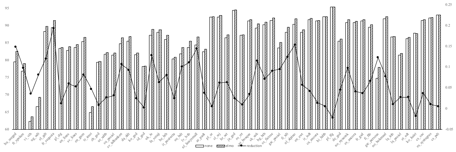
We study the effect of ELMo on the large treebanks and report the results of a single tagger and parser with and without ELMo. Figure 1(a) shows the tagging results on the development set and Figure 1(b) shows the parsing results. Using ELMo in the tagger leads to a macro-averaged improvement of 0.56% in UPOS and the macro-averaged error reduction is 17.83%. Using ELMo in the parser leads to a macro-averaged improvement of 0.84% in LAS and the macro-averaged error reduction is 7.88%.
ELMo improves the tagging performance almost on every treebank, except for zh_gsd and gl_ctg. Similar trends are witnessed in the parsing experiments with ko_kaist and pl_lfg being the only treebanks where ELMo slightly worsens the performance.
9.2 Effects of Ensemble
We also test the effect of ensemble and show the results in Figure 2. Parser ensemble leads to an averaged improvement of 0.55% in LAS and the averaged error reduction is 4.0%. These results indicate that ensemble is an effective way to improve the parsing performance. The relationship between gains using ensemble and treebank size is also studied in this figure and the trend is that small treebank benefit more from the ensemble. We address this to the fact that the ensemble improves the model’s generalization ability in which the parser trained on small treebank is weak due to overfitting.
9.3 Effects of Treebank Concatenation
As mentioned in Section 5, we study the effects of both the cross-domain concatenation and cross-lingual concatenation.
Cross-Domain Concatenation.
For the treebanks which have development set, the development performances are shown in Table 2. Numbers of sentences in the training set are also shown in this table. The general trend is that for the treebank with small training set, cross-domain concatenation achieves better performance. While for those with large training set, concatenation does not improve the performance or even worsen the results.
For the small treebanks which do not have development set, the 5 fold cross validation results are shown in Table 3 in which concatenation improves most of the treebanks except for gl_treegal.
Cross-Lingual Concatenation.
The experimental results of cross-lingual concatenation are shown in Table 4. Unfortunately, concatenating treebanks from different languages only achieves improved performance on uk_iu. This results also indicate that in cross lingual parsing, sophisticated methods like word embeddings transfer Guo et al. (2015); Guo et al. (2016b) and treebank transfer Guo et al. (2016a) are still necessary.
9.4 Effects of Better Preprocessing
| -sent. | udpipe | uppsala | |
| fi_tdt | +0.69 | 88.13 | 88.67 |
| et_edt | +1.22 | 86.33 | 86.36 |
| nl_lassysmall | +1.39 | 88.08 | 88.60 |
| da_ddt | +1.56 | 86.21 | 86.51 |
| el_gdt | +1.57 | 90.08 | 89.96 |
| cu_proiel | +1.72 | 72.79 | 74.04 |
| pt_bosque | +1.83 | 90.73 | 90.20 |
| id_gsd | +2.46 | 74.14 | 78.83 |
| la_proiel | +4.82 | 73.21 | 74.22 |
| got_proiel | +5.36 | 67.55 | 68.40 |
| grc_proiel | +5.86 | 79.67 | 80.72 |
| sl_ssj | +18.81 | 88.43 | 92.27 |
| it_postwita | +30.40 | 74.91 | 79.26 |
| -word | udpipe | scir | |
| ja_gsd | +4.07 | 80.53 | 85.23 |
| zh_gsd | +7.16 | 66.16 | 75.78 |
| vi_vtb | +9.02 | 48.58 | 57.53 |
| ltcode | sent+tokenize | tagger | parser | LAS | w/o ens. | ref. LAS |
|---|---|---|---|---|---|---|
| af_afribooms | udpipe: self | biaffine (none): self | biaffine (none)*3: self | 85.47 (1) | 84.41 (5) | 85.45 |
| ar_padt | udpipe: self | biaffine (): self | biaffine ()*3: self | 73.63 (2) | 73.34 (3) | 77.06 |
| bg_btb | udpipe: self | biaffine (): self | biaffine ()*3: self | 91.22 (1) | 90.89 (1) | 90.41 |
| br_keb | udpipe: self | biaffine_trans: self+ga_idt | biaffine_trans*3: self+ga_idt | 8.54 (21) | 7.82 (21) | 38.64 |
| bxr_bdt | udpipe: self | biaffine_trans: self+hi_hdtb | biaffine_trans*3: self+hi_hdtb | 15.44 (6) | 15.69 (6) | 19.53 |
| ca_ancora | udpipe: self | biaffine (): self | biaffine ()*3: self | 91.61 (1) | 91.29 (1) | 90.82 |
| cs_cac | udpipe: self | biaffine (): self | biaffine ()*3: self | 91.61 (1) | 91.33 (1) | 91.00 |
| cs_fictree | udpipe: self | biaffine (): self | biaffine ()*3: self | 92.02 (1) | 91.39 (3) | 91.83 |
| cs_pdt | udpipe: self | biaffine (): self | biaffine ()*3: self | 91.68 (1) | 91.45 (1) | 90.57 |
| cs_pud | udpipe: cs_pdt | biaffine (): cs_pdt | biaffine ()*3: cs_pdt | 86.13 (1) | 85.89 (1) | 85.35 |
| cu_proiel | uppsala: self | biaffine (): self | biaffine ()*3: self | 74.29 (3) | 73.29 (4) | 75.73 |
| da_ddt | uppsala: self | biaffine (): self | biaffine ()*3: self | 86.28 (1) | 85.54 (1) | 84.88 |
| de_gsd | udpipe: self | biaffine (): self | biaffine ()*3: self | 80.36 (1) | 79.81 (1) | 79.03 |
| el_gdt | uppsala: self | biaffine (): self | biaffine ()*3: self | 89.65 (1) | 88.88 (3) | 89.59 |
| en_ewt | udpipe: self | biaffine (): self | biaffine ()*3: self | 84.57 (1) | 83.88 (2) | 84.02 |
| en_gum | udpipe: self | biaffine (): self | biaffine ()*3: self | 84.42 (2) | 83.57 (2) | 85.05 |
| en_lines | udpipe: self | biaffine (): self | biaffine ()*3: self+en_ewt+en_gum | 81.97 (1) | 81.67 (1) | 81.44 |
| en_pud | udpipe: en_ewt | biaffine (): en_ewt | biaffine ()*3: en_ewt | 87.73 (2) | 87.26 (2) | 87.89 |
| es_ancora | udpipe: self | biaffine (): self | biaffine ()*3: self | 90.93 (1) | 90.62 (1) | 90.47 |
| et_edt | uppsala: self | biaffine (): self | biaffine ()*3: self | 85.35 (1) | 84.74 (1) | 84.15 |
| eu_bdt | udpipe: self | biaffine (): self | biaffine ()*3: self | 84.22 (1) | 83.42 (1) | 83.13 |
| fa_seraji | udpipe: self | biaffine (): self | biaffine ()*3: self | 88.11 (1) | 87.60 (1) | 86.18 |
| fi_ftb | udpipe: self | biaffine (): self | biaffine ()*3: self | 88.53 (1) | 88.00 (1) | 87.86 |
| fi_pud | udpipe: fi_tdt | biaffine (): fi_tdt | biaffine ()*3: fi_tdt | 90.23 (1) | 89.58 (1) | 89.37 |
| fi_tdt | uppsala: self | biaffine (): self | biaffine ()*3: self | 88.73 (1) | 88.68 (1) | 87.64 |
| fo_oft | udpipe: no_bokmaal | biaffine_trans: no_bokmaal | biaffine_trans*3: no_bokmaal | 44.05 (4) | 44.17 (4) | 49.43 |
| fr_gsd | udpipe: self | biaffine (): self | biaffine ()*3: self | 86.89 (1) | 86.81 (1) | 86.46 |
| fr_sequoia | udpipe: self | biaffine (): self | biaffine ()*3: self | 89.65 (2) | 89.12 (2) | 89.89 |
| fr_spoken | udpipe: self | biaffine (): self | biaffine ()*3: self+fr_gsd+fr_sequoia | 75.78 (1) | 75.09 (1) | 74.31 |
| fro_srcmf | udpipe: self | biaffine (none): self | biaffine (none)*3: self | 87.07 (2) | 86.53 (3) | 87.12 |
| ga_idt | udpipe: self | biaffine (none): self | biaffine (none)*3: self | 68.57 (5) | 66.80 (7) | 70.88 |
| gl_ctg | udpipe: self | biaffine (none): self | biaffine (none)*3: self | 82.35 (2) | 81.80 (3) | 82.76 |
| gl_treegal | udpipe: self | biaffine (none): self | biaffine (none)*3: self | 72.88 (4) | 71.27 (8) | 74.25 |
| got_proiel | uppsala: self | biaffine (none): self | biaffine (none)*3: self | 69.26 (3) | 67.61 (5) | 69.55 |
| grc_perseus | udpipe: self | biaffine (): self | biaffine ()*3: self | 79.39 (1) | 78.53 (1) | 74.29 |
| grc_proiel | uppsala: self | biaffine (): self | biaffine ()*3: self | 79.25 (1) | 78.35 (1) | 76.76 |
| he_htb | udpipe: self | biaffine (): self | biaffine ()*3: self | 67.05 (3) | 66.67 (3) | 76.09 |
| hi_hdtb | udpipe: self | biaffine (): self | biaffine ()*3: self | 92.41 (1) | 92.13 (1) | 91.75 |
| hr_set | udpipe: self | biaffine (): self | biaffine ()*3: self | 87.36 (1) | 86.82 (1) | 86.76 |
| hsb_ufal | udpipe: self | biaffine_trans: self+pl_lfg | biaffine_trans*3: self+pl_lfg | 37.68 (4) | 35.42 (4) | 46.42 |
| hu_szeged | udpipe: self | biaffine (): self | biaffine ()*3: self | 82.66 (1) | 80.96 (1) | 79.47 |
| hy_armtdp | udpipe: self | biaffine_trans: self+et_edt | biaffine_trans*3: self+et_edt | 33.90 (3) | 30.87 (3) | 37.01 |
| id_gsd | uppsala: self | biaffine (): self | biaffine ()*3: self | 80.05 (1) | 79.19 (1) | 79.13 |
| it_isdt | udpipe: self | biaffine (): self | biaffine ()*3: self | 92.00 (1) | 91.71 (1) | 91.47 |
| it_postwita | uppsala: self | biaffine (): self | biaffine ()*3: self+it_isdt | 79.39 (1) | 78.69 (1) | 78.62 |
| ja_gsd | udpipe+scir: self | biaffine (): self | biaffine ()*3: self | 83.11 (1) | 82.70 (1) | 79.97 |
| ja_modern | udpipe+scir: ja_gsd | biaffine (): ja_gsd | biaffine ()*3: ja_gsd | 26.58 (4) | 25.16 (4) | 28.33 |
| kk_ktb | udpipe: self | biaffine_trans: self+tr_imst | biaffine_trans*3: self+tr_imst | 23.92 (10) | 23.18 (13) | 31.93 |
| kmr_mg | udpipe: self | biaffine_trans: self+fa_seraji | biaffine_trans*3: self+fa_seraji | 26.26 (5) | 24.58 (6) | 30.41 |
| ko_gsd | udpipe: self | biaffine (): self | biaffine ()*3: self | 85.14 (1) | 84.76 (1) | 84.31 |
| ko_kaist | udpipe: self | biaffine (): self | biaffine ()*3: self | 86.91 (1) | 86.61 (2) | 86.84 |
| la_ittb | udpipe: self | biaffine (): self | biaffine ()*3: self | 87.08 (1) | 86.50 (2) | 86.54 |
| la_perseus | udpipe: self | biaffine (): self+la_proiel | biaffine ()*3: self+la_proiel | 72.63 (1) | 72.67 (1) | 68.07 |
| la_proiel | uppsala: self | biaffine (): self | biaffine ()*3: self | 73.61 (1) | 72.42 (1) | 71.76 |
| lv_lvtb | udpipe: self | biaffine (): self | biaffine ()*3: self | 83.97 (1) | 83.04 (1) | 81.85 |
| nl_alpino | udpipe: self | biaffine (): self | biaffine ()*3: self+nl_lassysmall | 89.56 (1) | 89.31 (1) | 87.49 |
| nl_lassysmall | uppsala: self | biaffine (): self | biaffine ()*3: self+nl_alpino | 86.84 (1) | 86.57 (1) | 84.27 |
| no_bokmaal | udpipe: self | biaffine (): self | biaffine ()*3: self | 91.23 (1) | 90.89 (1) | 90.37 |
| no_nynorsk | udpipe: self | biaffine (): self | biaffine ()*3: self | 90.99 (1) | 90.62 (1) | 89.46 |
| no_nynorsklia | udpipe: self | biaffine (): self+no_nynorsk | biaffine ()*3: self+no_nynorsk | 70.34 (1) | 69.06 (1) | 68.71 |
| pcm_nsc | udpipe: en_ewt | biaffine (): en_ewt | biaffine ()*3: en_ewt | 24.48 (2) | 25.16 (2) | 30.07 |
| pl_lfg | udpipe: self | biaffine (): self | biaffine ()*3: self | 94.86 (1) | 94.63 (1) | 94.62 |
| pl_sz | udpipe: self | biaffine (): self | biaffine ()*3: self | 92.23 (1) | 91.67 (1) | 91.59 |
| pt_bosque | uppsala: self | biaffine (): self | biaffine ()*3: self | 87.61 (3) | 87.32 (5) | 87.81 |
| ro_rrt | udpipe: self | biaffine (): self | biaffine ()*3: self | 86.87 (1) | 86.07 (3) | 86.33 |
| ru_syntagrus | udpipe: self | biaffine (): self | biaffine ()*3: self | 92.48 (1) | 92.26 (1) | 91.72 |
| ru_taiga | udpipe: self | biaffine (): self+ru_syntagrus | biaffine ()*3: self+ru_syntagrus | 71.81 (3) | 71.62 (3) | 74.24 |
| sk_snk | udpipe: self | biaffine (): self | biaffine ()*3: self | 88.85 (1) | 88.29 (1) | 87.59 |
| sl_ssj | uppsala: self | biaffine (): self | biaffine ()*3: self | 91.47 (1) | 91.08 (2) | 91.26 |
| sl_sst | udpipe: self | biaffine (): self | biaffine ()*3: self+sl_ssj | 61.39 (1) | 59.90 (1) | 58.12 |
| sme_giella | udpipe: self | biaffine (none): self | biaffine ()*3: self | 69.06 (3) | 67.43 (5) | 69.87 |
| sr_set | udpipe: self | biaffine (none): self | biaffine ()*3: self | 88.33 (3) | 87.78 (5) | 88.66 |
| sv_lines | udpipe: self | biaffine (): self | biaffine ()*3: self+sv_talbanken | 84.08 (1) | 83.64 (1) | 81.97 |
| sv_pud | udpipe: sv_lines | biaffine (): sv_lines | biaffine ()*3: sv_lines+sv_talbanken | 80.35 (1) | 79.78 (1) | 79.71 |
| sv_talbanken | udpipe: self | biaffine (): self | biaffine ()*3: self+sv_lines | 88.63 (1) | 88.26 (1) | 86.45 |
| th_pud | thai | biaffine_trans: zh_gsd | biaffine_trans*3: zh_gsd | 0.64 (14) | 0.61 (15) | 13.70 |
| tr_imst | udpipe: self | biaffine (): self | biaffine ()*3: self | 66.44 (1) | 64.91 (1) | 64.79 |
| ug_udt | udpipe: self | biaffine (): self | biaffine ()*3: self | 67.05 (1) | 66.20 (1) | 65.23 |
| uk_iu | udpipe: self | biaffine (): self | biaffine ()*3: self+ru_syntagrus | 88.43 (1) | 87.79 (1) | 85.16 |
| ur_udtb | udpipe: self | biaffine (): self | biaffine ()*3: self | 83.39 (1) | 82.17 (1) | 82.15 |
| vi_vtb | udpipe+scir: self | biaffine (): self | biaffine ()*3: self | 55.22 (1) | 53.92 (1) | 47.41 |
| zh_gsd | udpipe+scir: self | biaffine (none): self | biaffine ()*3: self | 76.77 (1) | 75.55 (1) | 71.04 |
| average | 75.84 (1) | 75.26 (1) |
We also study how preprocessing contributes to the final parsing performance. The experimental results on the development set are shown in Table 5. From this table, the performance of word segmentation is almost linearly correlated with the final performance. Similar trends on sentence segmentation performance are witnessed but el_gdt and pt_bosque presents some exceptions where better preprocess leads drop in the final parsing performance.
9.5 Parsing Strategies and Test Set Evaluation
Using the development set and cross validation, we choose the best model and data combination and the choices are shown in Table 6 along with the test evaluation. From this table, we can see that our system gains more improvements when both ELMo and parser ensemble are used. For some treebanks, concatenation also contributes to the improvements. Parsing Japanese, Vietnamese, and Chinese clearly benefits from better word segmentation. Since most of the participant teams use single parser for their system, we also remove the parser ensemble and do a post-contest evaluation. The results are also shown in this table. Our system without ensemble achieves an macro-averaged LAS of 75.26, which unofficially ranks the first according to LAS in the shared task.
We report the time and memory consumption. A full run over the 82 test sets on the TIRA virtual machine Potthast et al. (2014) takes about 40 hours and consumes about 4G RAM memory.
10 Conclusion
Our system submitted to the CoNLL 2018 shared task made several improvements on last year’s winning system from Dozat et al. (2017), including incorporating deep contextualized word embeddings, parser ensemble, and treebank concatenation. Experimental results on the development set show the effectiveness of our methods. Using these techniques, our system achieved an averaged LAS of 75.84% and obtained the first place in LAS in the final evaluation.
11 Credits
There are a few references we would like to give proper credit, especially to data providers: the core Universal Dependencies paper from LREC 2016 Nivre et al. (2016), the UD version 2.2 datasets Nivre et al. (2018), the baseline udpipe model released by Straka et al. (2016), the deep contextualized word embeddings code released by Peters et al. (2018), the biaffine tagger and parser released by Dozat et al. (2017), the joint sentence segmentor and tokenizer released by de Lhoneux et al. (2017), and the evaluation platform TIRA Potthast et al. (2014).
Acknowledgments
We thank the reviewers for their insightful comments, and the HIT-SCIR colleagues for the coordination on the machine usage. This work was supported by the National Key Basic Research Program of China via grant 2014CB340503 and the National Natural Science Foundation of China (NSFC) via grant 61300113 and 61632011.
References
- Ammar et al. (2016) Waleed Ammar, George Mulcaire, Miguel Ballesteros, Chris Dyer, and Noah Smith. 2016. Many languages, one parser. TACL 4.
- Björkelund et al. (2017) Anders Björkelund, Agnieszka Falenska, Xiang Yu, and Jonas Kuhn. 2017. Ims at the conll 2017 ud shared task: Crfs and perceptrons meet neural networks. In Proc. of the CoNLL 2017 Shared Task: Multilingual Parsing from Raw Text to Universal Dependencies. http://www.aclweb.org/anthology/K17-3004.
- Bojanowski et al. (2016) Piotr Bojanowski, Edouard Grave, Armand Joulin, and Tomas Mikolov. 2016. Enriching word vectors with subword information. CoRR abs/1607.04606. http://arxiv.org/abs/1607.04606.
- Che et al. (2017) Wanxiang Che, Jiang Guo, Yuxuan Wang, Bo Zheng, Huaipeng Zhao, Yang Liu, Dechuan Teng, and Ting Liu. 2017. The hit-scir system for end-to-end parsing of universal dependencies. In Proc. of the CoNLL 2017 Shared Task: Multilingual Parsing from Raw Text to Universal Dependencies. http://www.aclweb.org/anthology/K17-3005.
- de Lhoneux et al. (2017) Miryam de Lhoneux, Yan Shao, Ali Basirat, Eliyahu Kiperwasser, Sara Stymne, Yoav Goldberg, and Joakim Nivre. 2017. From raw text to universal dependencies - look, no tags! In Proc. of the CoNLL 2017 Shared Task: Multilingual Parsing from Raw Text to Universal Dependencies. http://www.aclweb.org/anthology/K17-3022.
- Dozat and Manning (2016) Timothy Dozat and Christopher D. Manning. 2016. Deep biaffine attention for neural dependency parsing. CoRR abs/1611.01734.
- Dozat et al. (2017) Timothy Dozat, Peng Qi, and Christopher D. Manning. 2017. Stanford’s graph-based neural dependency parser at the conll 2017 shared task. In Proc. of CoNLL 2017 Shared Task: Multilingual Parsing from Raw Text to Universal Dependencies.
- Guo et al. (2016a) Jiang Guo, Wanxiang Che, Haifeng Wang, and Ting Liu. 2016a. A universal framework for inductive transfer parsing across multi-typed treebanks. In Proc. of Coling. http://www.aclweb.org/anthology/C16-1002.
- Guo et al. (2015) Jiang Guo, Wanxiang Che, David Yarowsky, Haifeng Wang, and Ting Liu. 2015. Cross-lingual dependency parsing based on distributed representations. In Proc. of ACL.
- Guo et al. (2016b) Jiang Guo, Wanxiang Che, David Yarowsky, Haifeng Wang, and Ting Liu. 2016b. A representation learning framework for multi-source transfer parsing. In AAAI. pages 2734–2740.
- Jean et al. (2015) Sébastien Jean, Kyunghyun Cho, Roland Memisevic, and Yoshua Bengio. 2015. On using very large target vocabulary for neural machine translation. In Proc. of ACL. http://www.aclweb.org/anthology/P15-1001.
- Liu et al. (2018a) Yijia Liu, Wanxiang Che, Huaipeng Zhao, Bing Qin, and Ting Liu. 2018a. Distilling knowledge for search-based structured prediction. CoRR abs/1805.11224. http://arxiv.org/abs/1805.11224.
- Liu et al. (2018b) Yijia Liu, Yi Zhu, Wanxiang Che, Bing Qin, Nathan Schneider, and Noah A. Smith. 2018b. Parsing tweets into universal dependencies. In Proc. of NAACL. http://aclweb.org/anthology/N18-1088.
- Ma and Hovy (2017) Xuezhe Ma and Eduard Hovy. 2017. Neural probabilistic model for non-projective mst parsing. In Proc. of IJCNLP. http://www.aclweb.org/anthology/I17-1007.
- Ma et al. (2018) Xuezhe Ma, Zecong Hu, Jingzhou Liu, Nanyun Peng, Graham Neubig, and Eduard H. Hovy. 2018. Stack-pointer networks for dependency parsing. CoRR abs/1805.01087. http://arxiv.org/abs/1805.01087.
- Nivre et al. (2016) Joakim Nivre, Marie-Catherine de Marneffe, Filip Ginter, Yoav Goldberg, Jan Hajič, Christopher Manning, Ryan McDonald, Slav Petrov, Sampo Pyysalo, Natalia Silveira, Reut Tsarfaty, and Daniel Zeman. 2016. Universal Dependencies v1: A multilingual treebank collection. In Proc. of LREC-2016.
- Nivre et al. (2018) Joakim Nivre et al. 2018. Universal Dependencies 2.2. LINDAT/CLARIN digital library at the Institute of Formal and Applied Linguistics, Charles University, Prague, http://hdl.handle.net/11234/SUPPLYTHENEWPERMANENTIDHERE!
- Peters et al. (2018) Matthew Peters, Mark Neumann, Mohit Iyyer, Matt Gardner, Christopher Clark, Kenton Lee, and Luke Zettlemoyer. 2018. Deep contextualized word representations. In Proc. of NAACL. http://aclweb.org/anthology/N18-1202.
- Potthast et al. (2014) Martin Potthast, Tim Gollub, Francisco Rangel, Paolo Rosso, Efstathios Stamatatos, and Benno Stein. 2014. Improving the reproducibility of PAN’s shared tasks: Plagiarism detection, author identification, and author profiling. In Evangelos Kanoulas, Mihai Lupu, Paul Clough, Mark Sanderson, Mark Hall, Allan Hanbury, and Elaine Toms, editors, Information Access Evaluation meets Multilinguality, Multimodality, and Visualization. 5th International Conference of the CLEF Initiative (CLEF 14). Springer, Berlin Heidelberg New York, pages 268–299. https://doi.org/10.1007/978-3-319-11382-1_22.
- Reimers and Gurevych (2017) Nils Reimers and Iryna Gurevych. 2017. Reporting score distributions makes a difference: Performance study of lstm-networks for sequence tagging. In Proc. of EMNLP.
- Shao (2017) Yan Shao. 2017. Cross-lingual word segmentation and morpheme segmentation as sequence labelling. CoRR abs/1709.03756. http://arxiv.org/abs/1709.03756.
- Shi et al. (2017a) Tianze Shi, Liang Huang, and Lillian Lee. 2017a. Fast(er) exact decoding and global training for transition-based dependency parsing via a minimal feature set. In Proc. of EMNLP. https://www.aclweb.org/anthology/D17-1002.
- Shi et al. (2017b) Tianze Shi, Felix G. Wu, Xilun Chen, and Yao Cheng. 2017b. Combining global models for parsing universal dependencies. In Proc. of the CoNLL 2017 Shared Task: Multilingual Parsing from Raw Text to Universal Dependencies. http://www.aclweb.org/anthology/K17-3003.
- Smith et al. (2017) Samuel L. Smith, David H. P. Turban, Steven Hamblin, and Nils Y. Hammerla. 2017. Offline bilingual word vectors, orthogonal transformations and the inverted softmax. CoRR abs/1702.03859. http://arxiv.org/abs/1702.03859.
- Straka et al. (2016) Milan Straka, Jan Hajič, and Jana Straková. 2016. UDPipe: trainable pipeline for processing CoNLL-U files performing tokenization, morphological analysis, POS tagging and parsing. In Proc. of LREC-2016.
- Zeman et al. (2018) Daniel Zeman, Filip Ginter, Jan Hajič, Joakim Nivre, Martin Popel, and Milan Straka. 2018. CoNLL 2018 Shared Task: Multilingual Parsing from Raw Text to Universal Dependencies. In Proc. of the CoNLL 2018 Shared Task: Multilingual Parsing from Raw Text to Universal Dependencies.
- Zeman et al. (2017) Daniel Zeman, Martin Popel, Milan Straka, Jan Hajič, Joakim Nivre, Filip Ginter, Juhani Luotolahti, Sampo Pyysalo, Slav Petrov, Martin Potthast, Francis Tyers, Elena Badmaeva, Memduh Gökırmak, Anna Nedoluzhko, Silvie Cinková, Jan Hajič jr., Jaroslava Hlaváčová, Václava Kettnerová, Zdeňka Urešová, Jenna Kanerva, Stina Ojala, Anna Missilä, Christopher Manning, Sebastian Schuster, Siva Reddy, Dima Taji, Nizar Habash, Herman Leung, Marie-Catherine de Marneffe, Manuela Sanguinetti, Maria Simi, Hiroshi Kanayama, Valeria de Paiva, Kira Droganova, Héctor Martínez Alonso, Çağrı Çöltekin, Umut Sulubacak, Hans Uszkoreit, Vivien Macketanz, Aljoscha Burchardt, Kim Harris, Katrin Marheinecke, Georg Rehm, Tolga Kayadelen, Mohammed Attia, Ali Elkahky, Zhuoran Yu, Emily Pitler, Saran Lertpradit, Michael Mandl, Jesse Kirchner, Hector Fernandez Alcalde, Jana Strnadova, Esha Banerjee, Ruli Manurung, Antonio Stella, Atsuko Shimada, Sookyoung Kwak, Gustavo Mendonça, Tatiana Lando, Rattima Nitisaroj, and Josie Li. 2017. CoNLL 2017 Shared Task: Multilingual Parsing from Raw Text to Universal Dependencies.
- Zheng et al. (2017) Bo Zheng, Wanxiang Che, Jiang Guo, and Ting Liu. 2017. Enhancing lstm-based word segmentation using unlabeled data. In Chinese Computational Linguistics and Natural Language Processing Based on Naturally Annotated Big Data.