There are many reasons to believe that our current understanding of fundamental physics is incomplete. For example, the nature of dark matter and dark energy are still unknown, the stability of the Higgs mass remains unsolved, the origin of neutrino masses is unexplained, the strong CP problem is still there, the physics of inflation remains elusive, and the origin of the matter-antimatter asymmetry is still to be discovered. Attempts to address these shortcomings of the Standard Model (hereafter SM) often involve new degrees of freedom. These new particles can escape detection in terrestrial experiments either because they are too heavy to be produced at the energies available or because they are too weakly coupled to be created in sufficiently large numbers. However, in astrophysical systems and in the early universe the small cross sections can be compensated for by probing environments with large densities and by following the evolution over long time scales. For example, the high densities at the cores of stars allow a significant production of new weakly coupled species. Integrated over the long lifetime of stars this can lead to large deviations from the standard stellar evolution. Observations of the lifecycles of stars have therefore put interesting constraints on the couplings of new light species to the SM. Similarly, in the hot environment of the early universe, even extremely weakly coupled particles can be produced prolifically and their gravitational influence becomes detectable in the cosmic microwave background (CMB). Moreover, during inflation even very massive particles can be created by the rapid expansion of the spacetime. When these particles decay they produce distinctive signatures in cosmological observables. Observing these effects could teach us a great deal about the physics driving the inflationary expansion.

New physics can affect cosmological observables in two distinct ways: i ) it may affect the initial conditions of the hot big bang, or ii ) it may affect the evolution of these initial conditions through changes to the thermal history of the universe. These opportunities for probing new physics with cosmological observations are illustrated in the following schematic:

		new physics?
		$\displaystyle\hskip 113.81102pt\downarrow$
		evolution
		$\displaystyle\langle\zeta_{{\bf k}_{1}}\zeta_{{\bf k}_{2}}\ldots\rangle\ \xrightarrow{\ \hskip 113.81102pt\ }\ \langle O_{1}O_{2}\ldots\rangle$
		initial conditions cosmological correlators
		$\displaystyle\hskip 19.91684pt\uparrow$
		new physics?

where $\zeta$ denotes the primordial curvature perturbations and $O$ stands for late-time observables, which may be the temperature variations $\delta T$ of the CMB or the density fluctuations $\delta\rho_{g}$ in the distribution of galaxies. In these lectures, we will give examples from both of these avenues of tests for physics beyond the Standard Model (BSM).

The initial fluctuations were drawn from a probability distribution $P[\zeta]$ and hence are characterized by the following correlation functions

\langle\zeta_{{\bf k}_{1}}\zeta_{{\bf k}_{2}}\ldots\rangle=\int{\cal D}\zeta\,P[\zeta]\,\zeta_{{\bf k}_{1}}\zeta_{{\bf k}_{2}}\cdots\,.

By tracing the observed correlations $\langle O_{1}O_{2}\ldots\rangle$ back in time, cosmologists try to measure the initial correlations $\langle\zeta_{{\bf k}_{1}}\zeta_{{\bf k}_{2}}\ldots\rangle$ and use them to extract information about the initial probability distribution $P[\zeta]$ and about the physics that gave rise to it. If the early universe went through a period of inflation then these initial correlations were produced dynamically before the hot big bang. New physics during inflation, such as the existence of new degrees of freedom $X$ , can leave imprints in the spectrum of primordial perturbations, i.e. $P[\zeta]\to P[\zeta,X]$ .

New physics may also affect how the initial correlations evolve into the late-time observables. For example, the evolution equations for fluctuations in the primordial plasma can be affected by the presence of new degrees of freedom $X$ :

G_{\mu\nu}=8\pi G\left(T_{\mu\nu}^{\rm SM}+T_{\mu\nu}^{X}\right)\,,\qquad\nabla^{\mu}\left(T_{\mu\nu}^{\rm SM}+T_{\mu\nu}^{X}\right)=0\,.

As we will see, much of the evolution in the early universe is very well understood and probed by very precise observations. The possibilities for new physics are therefore highly constrained.

The most conservative way to parameterize physics beyond the Standard Model is in terms of an effective field theory (EFT). The basic input of an EFT are the field content and the symmetries that are relevant at a given energy scale. The effective Lagrangian is then the sum of all operators consistent with the symmetries,

{\cal L}_{\rm eff}\,\subset\,\sum g\,{\cal O}_{X}{\cal O}_{\rm SM}\,,

where ${\cal O}_{\rm SM}$ denotes operators made from the SM degrees of freedom and ${\cal O}_{X}$ stands for operators constructed from any additional fields. The couplings $g$ parameterize the strengths of the interactions between the fields $X$ and the SM. Deviations from the SM predictions then scale with the size of the couplings $g$ . In these lectures, I will show how cosmological observations put constraints on these couplings.

Outline

The goal of these lectures is to show that cosmology is becoming an increasingly sensitive probe of BSM physics. The presentation is divided into two parts: In Part I, we study the production of new light particles in the hot big bang and describe their effects on the anisotropies of the cosmic microwave background. In Part II, we investigate the possibility of very massive particles being created during inflation and determine their imprints in higher-order cosmological correlations.

Notation and conventions

Throughout these lectures, we will use natural units, $c=\hbar=1$ , with reduced Planck mass $M_{\rm pl}^{2}=1/8\pi G$ . Our metric signature is ( $-++\hskip 1.0pt+$ ). Greek letters will stand for spacetime indices, $\mu,\nu,\ldots=0,1,2,3$ , and Latin letters for spatial indices, $i,j,\ldots=1,2,3$ . Three-dimensional vectors will be written in boldface, ${\bf k}$ , and unit vectors will be hatted, $\hat{\bf k}$ . Overdots and primes will denote derivatives with respect to conformal time $\tau$ and physical time $t$ , respectively. The dimensionless power spectrum of a Fourier mode $\zeta_{\bf k}$ will be defined as

{\cal P}_{\zeta}(k)\equiv\frac{k^{3}}{2\pi^{2}}\langle\zeta_{\bf k}\zeta_{-{\bf k}}\rangle^{\prime}\,,

where the prime on the expectation value indicates that the overall momentum-conserving delta function has been dropped.

Acknowledgements

I am grateful to the organizers Igor Klebanov and Mirjam Cvetic for the invitation to lecture at TASI 2017. Thanks to my students and collaborators for many helpful discussions on the material presented in these lectures. I am especially grateful to Daniel Green, Joel Meyers, Benjamin Wallisch and Matias Zaldarriaga for collaboration on topics covered in Part I, and to Nima Arkani-Hamed, Valentin Assassi, Garrett Goon, Daniel Green, Hayden Lee, Liam McAllister and Guilherme Pimentel for collaboration on work described in Part II. Finally, thanks to Benjamin Wallisch and Swagat Saurav Mishra for comments on a preliminary version of the manuscript.

Part I Relics from the Hot Big Bang

Consider a $2\to N$ scattering process producing a new particle species $X$ . Assume that $X$ is very weakly coupled to the Standard Model degrees of freedom. The production of particles $X$ then carries energy and momentum away from the interaction region. Such missing energy, of course, famously led to the discovery of neutrinos. However, particles that are more weakly coupled than neutrinos are produced very rarely in colliders and their missing energy signatures are hard to detect. Fortunately, the creation of new species may be enhanced in astrophysical systems and in the early universe. To see this, consider the change in the number densities of the particles involved in the above interaction. Schematically, this is given by

\frac{\Delta n}{n}\sim n\sigma\times\Delta t\,,

i.e. the fractional change in the number density is equal to the interaction rate, $\Gamma\sim n\sigma$ , times the interaction time, $\Delta t$ . We see that small cross sections $\sigma$ can be compensated for by high densities and long time scales. This explains why observations of the lifecycles of stars have put interesting constraints on the existence of extra species. Taking the typical number density inside of stars to be $n\sim(1\,{\rm keV})^{3}$ and integrating over the typical lifetime of a star, $\Delta t\sim 10^{16}\,{\rm sec}\approx 1.5\times 10^{31}\,{\rm eV}^{-1}$ , we find significant changes in the stellar evolution if

\sigma>(n\Delta t)^{-1}\sim(10^{10}\,{\rm GeV})^{-2}\,.

Similar constraints can be derived from the observed energy loss in supernova explosions. In that case, the relevant time scales are much shorter, $\Delta t\sim 10\,{\rm sec}$ , but the densities are much higher, $n\sim(30\,{\rm MeV})^{3}$ .

These order of magnitude estimates also give us a sense for the power of cosmological constraints. In the early universe, the interaction time scales are short, $\Delta t<1\,{\rm sec}$ , but the densities can be very high, $n\sim T^{3}\gg(1\,{\rm MeV})^{3}$ . For temperatures above $10^{4}\,{\rm GeV}$ , we expect cosmological constraints to be stronger than those from astrophysics. In this part of the lectures, we will show that primordial cosmology is indeed a highly sensitive probe of new light particles produced in the hot Big Bang.

We will begin, in Section 2, with a quick review of FRW cosmology. In Section 3, we will introduce the cosmic microwave background as a tool for precision cosmology. In Section 4, we will discuss the physics of the acoustic oscillations observed in the CMB anisotropy spectrum. Finally, in Section 5, we will show that extra relativistic particles leave a unique signature in the CMB spectrum.

2 Big Bang Cosmology

We will begin with a lightning review of some elementary concepts in cosmology. I will assume that you have seen most, if not all, of this material before, so I will cite many results without detailed derivations. Further details can be found in my Cosmology course [1] or in any of the standard textbooks (e.g. [2, 3]).

2.1 Geometry and Dynamics

The Friedmann-Robertson-Walker (FRW) metric of a homogenous and isotropic spacetime is

{\rm d}s^{2}=-{\rm d}t^{2}+a^{2}(t)\gamma_{ij}\hskip 1.0pt{\rm d}x^{i}{\rm d}x^{j}\,,

(2.1)

where $\gamma_{ij}$ denotes the metric of a maximally symmetric 3-space and $a(t)$ is the scale factor. Throughout these lectures, we will restrict to the special case of flat spatial slices, i.e. $\gamma_{ij}=\delta_{ij}$ , and define ${\rm d}{\bf{x}}^{2}\equiv\delta_{ij}{\rm d}x^{i}{\rm d}x^{j}$ . We will also introduce conformal time, ${\rm d}\tau={\rm d}t/a(t)$ , so that the metric becomes

{\rm d}s^{2}=a^{2}(\tau)\left(-{\rm d}\tau^{2}+{\rm d}{\bf{x}}^{2}\right).

(2.2)

We will first discuss the kinematics of particles in an FRW spacetime for an arbitrary scale factor $a(\tau)$ . After that, we will show how the Einstein equations determine $a(\tau)$ in terms of the matter content of the universe.

Kinematics

Particles in the FRW spacetime evolve according to the geodesic equation

P^{\nu}\nabla_{\nu}P^{\mu}=P^{\nu}\left(\frac{\partial P^{\mu}}{\partial x^{\nu}}+\Gamma^{\mu}_{\nu\rho}\hskip 1.0ptP^{\rho}\right)=0\,,

(2.3)

where $P^{\mu}\equiv dx^{\mu}/d\lambda$ is the four-momentum of the particle. In an expanding spacetime, it is convenient to write the components of the four-momentum as

P^{\mu}=a^{-1}[E,{\bf{p}}]\,.

(2.4)

For massless particles, such as photons, we have the constraint $g_{\mu\nu}P^{\mu}P^{\nu}=-E^{2}+|{\bf{p}}|^{2}=0$ , so we can write ${\bf{p}}=E\hskip 1.0pt{\hat{\bf p}}$ , where ${\hat{\bf p}}$ is a unit vector in the direction of propagation.

Exercise.—Show that the non-zero connection coefficients associated with the metric (2.2) are

\Gamma^{0}_{00}={\cal H}\,,\hskip 9.24994pt\Gamma^{0}_{ij}={\cal H}\delta_{ij}\,,\hskip 9.24994pt\Gamma^{i}_{j0}={\cal H}\delta^{i}_{j}\,,

(2.5)

where ${\cal H}\equiv\dot{a}/a$ is the conformal Hubble parameter.

The $\mu=0$ component of the geodesic equation (2.3) becomes

P^{0}\frac{dP^{0}}{d\tau}=-\Gamma^{0}_{\alpha\beta}P^{\alpha}P^{\alpha}\,.

(2.6)

Using (2.4) and (2.5), we get

(a^{-1}E)\frac{d}{d\tau}(a^{-1}E)=-{\cal H}a^{-2}E^{2}-{\cal H}a^{-2}|{\bf{p}}|^{2}\,,

(2.7)

which simplifies to

\frac{1}{E}\frac{dE}{d\tau}=-\frac{1}{a}\frac{da}{d\tau}\,.

(2.8)

This describes the redshifting of the photon energy in an expanding spacetime, $E\propto a^{-1}$ .

Dynamics

The evolution of the scale factor is determined by the Friedmann equations

	$\displaystyle 3{\cal H}^{2}$	$\displaystyle=8\pi Ga^{2}\bar{\rho}\,,$		(2.9)
	$\displaystyle 2\dot{\cal H}+{\cal H}^{2}$	$\displaystyle=-8\pi Ga^{2}\,\bar{P}\,,$		(2.10)

where $\bar{\rho}$ and $\bar{P}$ are the background density and pressure, respectively.

Exercise.—By substituting (2.5) into

R_{\mu\nu}\equiv\partial_{\lambda}\Gamma^{\lambda}_{\mu\nu}-\partial_{\nu}\Gamma^{\lambda}_{\mu\lambda}+\Gamma^{\lambda}_{\lambda\rho}\Gamma^{\rho}_{\mu\nu}-\Gamma^{\rho}_{\mu\lambda}\Gamma^{\lambda}_{\nu\rho}\ ,

(2.11)

show that

R_{00}=-3\dot{\cal H}\,,\hskip 9.24994ptR_{ij}=(\dot{\cal H}+2{\cal H}^{2})\delta_{ij}\hskip 9.24994pt\Rightarrow\hskip 9.24994pta^{2}R\equiv a^{2}g^{\mu\nu}R_{\mu\nu}=-6(\dot{\cal H}+{\cal H}^{2})\,.

(2.12)

Hence, show that the non-zero components of the Einstein tensor, $G_{\mu\nu}\equiv R_{\mu\nu}-\frac{1}{2}Rg_{\mu\nu}$ , are

G_{00}=3{\cal H}^{2}\,,\ \hskip 9.24994ptG_{ij}=-(2\dot{\cal H}+{\cal H}^{2})\delta_{ij}\,.\phantom{\hskip 9.24994pt\Rightarrow\hskip 110.96556pt\hskip 9.24994pt\hskip 18.49988ptx}

(2.13)

Use this to confirm that the $00$ -Einstein equation, $G_{00}=8\pi G\hskip 1.0ptT_{00}$ , implies (2.9) and the $ij$ -Einstein equation, $G_{ij}=8\pi G\hskip 1.0ptT_{ij}$ , leads to (2.10).

Combining (2.9) and (2.10), we can write an evolution equation for the density

\dot{\bar{\rho}}=-3{\cal H}(\bar{\rho}+\bar{P})\,.

(2.14)

For pressureless matter ( $\bar{P}_{m}\approx 0$ ) this implies $\bar{\rho}_{m}\propto a^{-3}$ , while for radiation ( $\bar{P}_{r}=\frac{1}{3}\bar{\rho}_{r}$ ) we have $\bar{\rho}_{r}\propto a^{-4}$ .

Exercise.—Derive the continuity equation (2.14) from the conservation of the stress tensor, $\nabla^{\mu}T_{\mu\nu}=0$ . By integrating the Friedmann equation (2.9) for matter and radiation show that

a(\tau)=\left\{\begin{array}[]{ll}\tau^{2}&\ {\rm matter}\\[4.0pt] \tau&\ {\rm radiation}\end{array}\right.\,.

(2.15)

Cosmic inventory

The universe is filled with several different species of particles:

\underbrace{\ \small{\rm photons}\ (\gamma)\hskip 9.24994pt{\rm neutrinos}\ (\nu)\ }_{\displaystyle{\small\rm radiation}\ (r)}\hskip 9.24994pt\underbrace{\overbrace{\ {\rm electrons}\ (e)\hskip 9.24994pt{\rm protons}\ (p)\ }^{\displaystyle{\rm baryons}\ (b)}\hskip 9.24994pt\text{cold dark matter}\ (c)\ }_{\displaystyle{\rm matter}\ (m)}\ .

The number density, energy density and pressure of each species $a$ can be written as

$\displaystyle n_{a}$	$\displaystyle=g_{a}\int\frac{{\rm d}^{3}p}{(2\pi)^{3}}\,f_{a}({\bf{x}},{\bf{p}})\,,$	(2.16)
$\displaystyle\rho_{a}$	$\displaystyle=g_{a}\int\frac{{\rm d}^{3}p}{(2\pi)^{3}}\,f_{a}({\bf{x}},{\bf{p}})\hskip 1.0ptE(p)\,,$	(2.17)
$\displaystyle P_{a}$	$\displaystyle=g_{a}\int\frac{{\rm d}^{3}p}{(2\pi)^{3}}\,f_{a}({\bf{x}},{\bf{p}})\hskip 1.0pt\frac{p^{2}}{3E(p)}\,,$	(2.18)

where $f_{a}({\bf{x}},{\bf{p}})$ is the (phase space) distribution function of the species $a$ , and $g_{a}$ is the number of internal degrees of freedom. In the unperturbed universe, the distribution functions should not depend on the position and the direction of the momentum, i.e. $f_{a}({\bf{x}},{\bf{p}})\to\bar{f}_{a}(E(p))$ .

At early times, particle interactions were efficient enough to keep the different species in local equilibrium. They then shared a common temperature $T$ and the distribution functions take the following maximum entropy form

\bar{f}_{a}(E)=\frac{1}{e^{(E_{a}-\mu_{a})/T}\pm 1}\,,

(2.19)

with $+$ for fermions and $-$ for bosons. The chemical potential $\mu_{a}$ vanishes for photons and is (likely) small for all other species. We will henceforth set it to zero. When the temperature drops below the mass of a particle species, $T\ll m_{a}$ , they become non-relativistic and their distribution function receives an exponential (Boltzmann) suppression, $f_{a}\to e^{-m_{a}/T}$ . This means that relativistic particles (‘radiation’) dominate the density and pressure of the primordial plasma. By performing the integrals (2.17) and (2.18) in the limit $E\to p$ , one finds

\bar{\rho}_{a}=\frac{\pi^{2}}{30}\,g_{a}\hskip 1.0ptT^{4}\,\left\{\begin{array}[]{ll}1&\ {\rm bosons}\\[4.0pt] \frac{7}{8}&\ {\rm fermions}\end{array}\right.\quad{\rm and}\quad\bar{P}_{a}=\frac{1}{3}\bar{\rho}_{a}\,.

(2.20)

The total radiation density is

\bar{\rho}_{r}=\frac{\pi^{2}}{30}\,g_{*}\hskip 1.0ptT^{4}\,,\quad\text{where}\quad g_{*}\equiv\sum_{a=b}g_{a}+\frac{7}{8}\,\sum_{a=f}g_{a}\,.

(2.21)

If equilibrium had persisted until today, all species with masses greater than $10^{-3}$ eV would be exponentially suppressed. This would not be a very interesting world. Fortunately, many massive particle species (e.g. dark matter) are weakly interacting and decoupled from the primordial plasma at early times.

2.2 Thermal History

The key to understanding the thermal history of the universe is understanding the competition between the interaction rate of particles, $\Gamma$ , and the expansion rate of the universe, $H$ . Particles maintain equilibrium as long as $\Gamma\gg H$ and freeze out when $\Gamma\lesssim H$ (see Fig. 1).

Figure 1: A schematic illustration of particle freeze-out. At high temperatures, the particle abundance tracks its equilibrium value. At low temperatures, the particles freeze out and maintain a relic density that is much larger than the Boltzmann-suppressed equilibrium abundance.

Neutrinos are the most weakly interacting particles of the Standard Model and therefore decoupled first (around $0.8$ MeV or $1$ sec after the Big Bang). Shortly after neutrino decoupling, electrons and positrons annihilated. The energies of the electrons and positrons got transferred to the photons, but not the neutrinos. The temperature of the photons today is therefore slightly larger than that of the neutrinos (see insert below). At around the same time, neutron-proton interactions became inefficient, leading to a relic abundance of neutrons. These neutrons were essential for the formation of the light elements during Big Bang nucleosynthesis (BBN), which occurred around 3 minutes after the Big Bang.

Figure 2: Thermal history through electron-positron annihilation. Neutrinos are decoupled and their temperature redshifts simply as

T_{\nu}\propto a^{-1}

. The energy density of the electron-positron pairs is transferred to the photon gas whose temperature therefore redshifts more slowly,

T_{\gamma}\propto g_{*}^{-1/3}a^{-1}

Cosmic neutrino background. After the neutrinos decouple, their momenta redshift, $p_{\nu}\propto a^{-1}$ , and their distribution functions $f_{\nu}$ maintain their shape. The combination of these two facts requires that the neutrino temperature evolves as $T_{\nu}\propto a^{-1}$ . We would like to compare this to the evolution of the photon temperature $T_{\gamma}$ , since this is what has been measured by observations of the CMB. We will use the fact that the comoving entropy is conserved in equilibrium [1]:

sa^{3}=\frac{\rho+P}{T}a^{3}=\frac{2\pi^{2}}{45}g_{*}(aT)^{3}=const\,.

(2.22)

Since entropy is separately conserved for the thermal bath and the decoupled species, we only need to consider the change in the effective number of relativistic degrees of freedom in equilibrium with the photons. Before $e^{+}e^{-}$ annihilation, i.e. at $T_{+}>m_{e}$ , we have

g_{*}(T_{+})=2+\frac{7}{8}\times(2\times 2)=\frac{11}{2}\,,

(2.23)

where we have counted photons, electrons and positrons. After $e^{+}e^{-}$ annihilation, i.e. at $T_{-}<m_{e}$ , only the two polarization degrees of freedom of the photons contribute,

\hskip-88.2037ptg_{*}(T_{-})=2\,.

(2.24)

Comparing $g_{*}(aT_{\gamma})^{3}={const.}$ to $aT_{\nu}={const.}$ , we get

T_{\nu}=\left(\frac{g_{*}(T_{-})}{g_{*}(T_{+})}\right)^{1/3}T_{\gamma}=\left(\frac{4}{11}\right)^{1/3}T_{\gamma}\,.

(2.25)

Given the measured temperature of the CMB today, $T_{\gamma,0}=2.7\,{\rm K}$ , this tells us that the present temperature of the cosmic neutrino background (C $\nu$ B) is $T_{\nu,0}=1.9\,{\rm K}$ .

While the neutrinos are still relativistic (i.e. for most of the history of the universe), each species carries the following energy density

\frac{\rho_{\nu}}{\rho_{\gamma}}=\frac{\frac{7}{8}\times 2\times T_{\nu}^{4}}{\phantom{\frac{7}{8}\times\ }2\times T_{\gamma}^{4}}=\frac{7}{8}\left(\frac{4}{11}\right)^{4/3}\equiv a_{\nu}\approx 0.227\,.

(2.26)

The $N_{\nu}=3$ neutrino species of the Standard Model therefore contribute a significant amount to the total radiation density in the early universe:

\displaystyle\frac{\sum\rho_{\nu}}{\rho_{r}}=\frac{N_{\nu}\rho_{\nu}}{N_{\nu}\rho_{\nu}+\rho_{\gamma}}=\frac{N_{\nu}a_{\nu}}{N_{\nu}a_{\nu}+1}\,\approx\,41\%\,.

(2.27)

Although the neutrinos are decoupled, their gravitational effects are significant and have recently been observed in the CMB [4, 5].

Below about 1 eV, or 380,000 years after the Big Bang, the temperature became low enough for neutral hydrogen atoms to form through the reaction $e^{-}+p^{+}\to{\rm H}+\gamma$ . This is the moment of recombination. At this point the density of free electrons dropped dramatically. Before recombination the strongest coupling between the photons and the rest of the plasma was through Thomson scattering, $e^{-}+\gamma\to e^{-}+\gamma$ . The sharp drop in the free electron density after recombination means that this process became inefficient and the photons decoupled. After decoupling the photons streamed freely through the universe and are observed today as the CMB.

Refer to caption — Figure 3: Planck measurement of the temperature variations in the CMB sky.

2.3 Structure Formation

The CMB is an almost perfect blackbody with an average temperature of 2.7 K. Small variations in the CMB temperature across the sky (see Fig. 3), reflect spatial variations in the density of the primordial plasma, $\delta\rho_{a}\equiv\rho_{a}-\bar{\rho}_{a}$ (see Section 3), and related perturbations of the spacetime geometry, $\delta g_{\mu\nu}\equiv g_{\mu\nu}-\bar{g}_{\mu\nu}$ . During the radiation-dominated phase of the early universe, the growth of matter perturbations was inhibited by the large pressure provided by the radiation. Perturbations in the coupled photon and baryon fluids were oscillating with constant amplitude (see Section 4). Shortly before recombination, however, the universe became matter dominated and the radiation pressure disappeared, so that density fluctuations could start to grow under the influence of gravity. This growth of the matter perturbations eventually led to the large-scale structure (LSS) of the universe.

2.4 Initial Conditions

At sufficiently early times, all scales of interest to current observations were outside the Hubble radius, $k<{\cal H}$ . On super-Hubble scales, the evolution of perturbations becomes very simple, especially for adiabatic initial conditions.

Adiabatic perturbations

Adiabatic perturbations have the property that the local state of matter (determined, for example, by the energy density $\rho$ and the pressure $P$ ) at some spacetime point ( $\tau,{\bf{x}}$ ) of the perturbed universe is the same as in the background universe at some slightly different time $\tau+\delta\tau({\bf{x}})$ . (Notice that the time shift varies with position ${\bf{x}}$ .) If the universe is filled with multiple fluids, adiabatic perturbations correspond to perturbations induced by a common, local shift in time of all background quantities; e.g. adiabatic density perturbations are defined as

\delta\rho_{a}(\tau,{\bf{x}})\equiv\bar{\rho}_{a}(\tau+\delta\tau({\bf{x}}))-\bar{\rho}_{a}(\tau)\approx\dot{\bar{\rho}}_{a}\hskip 1.0pt\delta\tau({\bf{x}})\,,

(2.28)

where $\delta\tau$ is the same for all species $a$ . This implies that all matter perturbations can be characterized by a single degree of freedom. It also means that we can perform a local time reparameterization to set all matter perturbations to zero, e.g. $\delta\rho_{a}\equiv 0$ . In that gauge, the information about fluctuations is carried by the following perturbation of the metric

g_{ij}(\tau,{\bf{x}})=a^{2}(\tau)\,e^{2\zeta(\tau,{\bf{x}})}\,\delta_{ij}\,,

(2.29)

where $\zeta$ is called the curvature perturbation. An attractive property of the curvature perturbation is that it is conserved on super-Hubble scales.

Statistics

The initial conditions for the hot Big Bang are believed to have been created by quantum fluctuations during a period of inflationary expansion [6]. As we will see in Section 7, this mechanism predicts the statistics of the initial conditions, i.e. it predicts the correlations between the CMB fluctuations in different directions in the sky, rather than the specific value of the temperature fluctuation in a specific direction. For Gaussian initial conditions, these correlations are completely specified by the two-point correlation function

\langle\zeta({\bf{x}})\zeta({\bf{x}}^{\prime})\rangle\equiv\xi_{\zeta}({\bf{x}},{\bf{x}}^{\prime})=\xi_{\zeta}(|{\bf{x}}^{\prime}-{\bf{x}}|)\,,

(2.30)

where the last equality holds as a consequence of statistical homogeneity and isotropy. The Fourier transform of $\zeta$ then satisfies

\langle\zeta({\bf k})\zeta^{*}({\bf k}^{\prime})\rangle=\frac{2\pi^{2}}{k^{3}}{\cal P}_{\zeta}(k)\,\delta_{D}({\bf k}-{\bf k}^{\prime})\,,

(2.31)

where ${\cal P}_{\zeta}(k)$ is the (dimensionless) power spectrum.

Exercise.—Show that

\xi_{\zeta}({\bf{x}},{\bf{x}}^{\prime})\,=\,\int\frac{{\rm d}k}{k}\,{\cal P}_{\zeta}(k)\,{\rm sinc}(k|{\bf{x}}-{\bf{x}}^{\prime}|)\,.

(2.32)

In Section 7, we will explicitly compute the form of ${\cal P}_{\zeta}(k)$ predicted by inflation. However, before we do that, we will show, in Sections 3 and 4, how generic scale-invariant initial conditions, ${\cal P}_{\zeta}(k)\approx const.$ , evolve into the anisotropies of the cosmic microwave background. We will first do this in the context of the Standard Model of particle physics, before asking, in Section 5, what kind of deviations can arise in theories beyond the SM.

3 Afterglow of the Big Bang

Observations of the temperature fluctuations in the cosmic microwave background have played a pivotal role in establishing the standard cosmological model. We now have a detailed understanding of the geometry and composition of the universe, and there is growing evidence that the primordial fluctuations originated from quantum fluctuations during a period of inflation. In this section and the next, we will give a simplified analytical treatment of the physics of the CMB anisotropies. Our goal is to present just enough details to be able to explain how the CMB can be used as a probe of BSM physics.

3.1 CMB Anisotropies

The first thing one sees when looking at the microwave scy is the motion of the Solar System with respect to the rest frame of the CMB (cf. Fig. 4).

Figure 4: The motion of the Solar System relative to the CMB rest frame produces a dipolar pattern in the observed CMB temperature.

Consider a photon entering our detectors from a direction $\hat{\bf n}$ . In the rest frame of the CMB, it has momentum ${\bf{p}}=-p\hskip 1.0pt\hat{\bf n}$ . Due to the Doppler effect, the observed momentum is

p_{0}(\hat{\bf n})=\frac{p}{\gamma(1-\hat{\bf n}\cdot{\bf{v}})}\approx p\left(1+\hat{\bf n}\cdot{\bf{v}}\right),

(3.1)

where ${\bf{v}}$ is our velocity relative to the CMB rest frame, $p$ is the momentum of the photon in the CMB rest frame and $\gamma=(1-v^{2})^{-1/2}$ is the Lorentz factor. We have also shown an approximation at leading order in $|{\bf{v}}|\ll 1$ . As expected, the momentum is higher if we move towards the photon ( $\hat{\bf n}\cdot{\bf{v}}=v$ ) and smaller if we move away from it ( $\hat{\bf n}\cdot{\bf{v}}=-v$ ). Since the CMB has a blackbody spectrum, we can relate the change in the observed momentum of photons to a change in the observed temperature:

\frac{\delta T(\hat{\bf n})}{T}\equiv\frac{T_{0}(\hat{\bf n})-T}{T}=\frac{p_{0}(\hat{\bf n})-p}{p}=\hat{\bf n}\cdot{\bf{v}}=v\cos\theta\,.

(3.2)

Fitting this dipolar anisotropy to the data, we find that the speed of the Solar System relative to the CMB is

v=368\,{\rm km}/{\rm s}\ .

(3.3)

After subtracting the dipole, we are left with the primordial anisotropy.

Perturbed photon geodesics

Let us trace the life of a photon after decoupling. Its (physical) momentum will redshift due to the expansion of the universe. In addition, the momentum will change in response to the inhomogeneities of the universe. We will study these effects by solving the geodesic equation (2.3) in the perturbed spacetime.

We will treat perturbations in the metric in (conformal) Newtonian gauge

{\rm d}s^{2}=a^{2}(\tau)\big[-(1+2\Phi){\rm d}\tau^{2}+(1-2\Psi)\delta_{ij}{\rm d}x^{i}{\rm d}x^{j}\big]\,,

(3.4)

where the perturbation $\Phi\approx\Psi$ plays the role of the gravitational potential.

Exercise.—Show that the connection coefficients associated with the metric (3.4) are

$\displaystyle\Gamma^{0}_{00}$	$\displaystyle={\cal H}+\dot{\Phi}\,,$	(3.5)
$\displaystyle\Gamma^{0}_{i0}$	$\displaystyle=\partial_{i}\Phi\,,$
$\displaystyle\Gamma^{i}_{00}$	$\displaystyle=\delta^{ij}\partial_{j}\Phi\,,$
$\displaystyle\Gamma^{0}_{ij}$	$\displaystyle={\cal H}\delta_{ij}-\big[\dot{\Psi}+2{\cal H}(\Phi+\Psi)\big]\delta_{ij}\,,$
$\displaystyle\Gamma^{i}_{j0}$	$\displaystyle=\big[{\cal H}-\dot{\Psi}\big]\delta^{i}_{j}\,,$
$\displaystyle\Gamma^{i}_{jk}$	$\displaystyle=-2\delta^{i}_{(j}\partial_{k)}\Psi+\delta_{jk}\delta^{il}\partial_{l}\Psi\,.$

As we will show in the following insert, the geodesic equation then leads to the following evolution equation for the photon momentum:

\framebox{$\displaystyle\frac{d}{d\tau}\ln(ap)=-\frac{d\Phi}{d\tau}+\frac{\partial(\Phi+\Psi)}{\partial\tau}$}\ .

(3.6)

In the absence of the source terms on the right-hand side, this implies $p\propto a^{-1}$ , which is the expected redshifting due to the expansion of the universe, cf. eq. (2.8). The inhomogeneous source terms describe how photons lose (gain) energy as they move out of (into) potential wells.

Derivation.—We will derive eq. (3.6) from the geodesic equation for photons,

\frac{dP^{0}}{d\lambda}=-\Gamma^{0}_{\alpha\beta}P^{\alpha}P^{\beta}\,,

(3.7)

where $P^{\mu}=dx^{\mu}/d\lambda$ is the four-momentum of the photons. We need expressions for the components of the four-momentum in the presence of metric perturbations.

•

We first consider the $P^{0}$ component. Since photons are massless we have

$\displaystyle P^{2}=g_{\mu\nu}P^{\mu}P^{\nu}$ $\displaystyle=0$

$\displaystyle=-a^{2}(1+2\Phi)(P^{0})^{2}+p^{2}\,,$ (3.8)

where we have substituted the metric (3.4) and defined $p^{2}\equiv g_{ij}P^{i}P^{j}$ . Solving (3.8) for $P^{0}$ , we find

$P^{0}=\frac{p}{a}(1-\Phi)\,.$ (3.9)

•

We then write the spatial component of the four-momentum as

P^{i}\equiv\alpha\,\hat{p}^{i}\,.

(3.10)

To determine the constant of proportionality $\alpha$ , we use

	$\displaystyle p^{2}=g_{ij}P^{i}P^{j}$	$\displaystyle=a^{2}(1-2\Psi)\delta_{ij}\hat{p}^{i}\hat{p}^{j}\alpha^{2}$
		$\displaystyle=a^{2}(1-2\Psi)\alpha^{2}\,,$		(3.11)

where the last equality holds because the direction vector is a unit vector. Solving (3.11) for $\alpha$ , we get $\alpha=p(1+\Psi)/a$ , or

P^{i}=\frac{p\hat{p}^{i}}{a}(1+\Psi)\,.

(3.12)

Substituting these results into the geodesic equation (3.7), we get

\frac{p}{a}(1-\Phi)\frac{d}{d\tau}\left[\frac{p}{a}(1-\Phi)\right]=-\Gamma^{0}_{\alpha\beta}P^{\alpha}P^{\beta}\,,

(3.13)

where we have used the standard trick of rewriting the derivative with respect to $\lambda$ as a derivative with respect to time multiplied by $d\tau/d\lambda=P^{0}$ . We expand out the time derivative to get

\frac{dp}{d\tau}(1-\Phi)={\cal H}p(1-\Phi)+p\frac{d\Phi}{d\tau}-\Gamma^{0}_{\alpha\beta}P^{\alpha}P^{\beta}\,\frac{a^{2}}{p}(1+\Phi)\,.

(3.14)

Multiplying both sides by $(1+\Phi)/p$ and dropping all quadratic terms in $\Phi$ , we find

\frac{1}{p}\frac{dp}{d\tau}={\cal H}+\frac{d\Phi}{d\tau}-\Gamma^{0}_{\alpha\beta}P^{\alpha}P^{\beta}\,\frac{a^{2}}{p^{2}}(1+2\Phi)\,.

(3.15)

To evaluate the last term on the right-hand side, we use the perturbed Christoffel symbols (3.5). After a bit of algebra, we get

-\Gamma^{0}_{\alpha\beta}\frac{P^{\alpha}P^{\beta}}{p^{2}}(1+2\Phi)=-2{\cal H}+\frac{\partial\Psi}{\partial\tau}-\frac{\partial\Phi}{\partial\tau}-2\hskip 1.0pt\hat{p}^{i}\frac{\partial\Phi}{\partial x^{i}}\,.

(3.16)

Equation (3.15) then becomes

\displaystyle\frac{1}{p}\frac{dp}{dt}

\displaystyle=-{\cal H}+\frac{d\Phi}{d\tau}-2\left(\frac{\partial\Phi}{\partial\tau}+\hat{p}^{i}\frac{\partial\Phi}{\partial x^{i}}\right)+\frac{\partial(\Phi+\Psi)}{\partial\tau}\,.

(3.17)

At leading order, the term in brackets is equal to the total time derivative of $\Phi$ :

\frac{d\Phi}{d\tau}=\frac{\partial\Phi}{\partial\tau}+\frac{dx^{i}}{d\tau}\frac{\partial\Phi}{\partial x^{i}}=\frac{\partial\Phi}{\partial\tau}+\hat{p}^{i}\frac{\partial\Phi}{\partial x^{i}}\,,

(3.18)

where we used

\frac{dx^{i}}{d\tau}=\frac{dx^{i}}{d\lambda}\frac{d\lambda}{d\tau}=\frac{P^{i}}{P^{0}}=\hat{p}^{i}(1+\Psi+\Phi)=\hat{p}^{i}+{\cal O}(1)\,.

(3.19)

Substituting (3.18) into (3.17), we get

\frac{1}{p}\frac{dp}{d\tau}=-\frac{1}{a}\frac{da}{d\tau}-\frac{d\Phi}{d\tau}+\frac{\partial(\Phi+\Psi)}{\partial\tau}\,,

(3.20)

which confirms the result (3.6).

Line-of-sight solution

By integrating the geodesic equation (3.6) along a line-of-sight, we can relate the observed CMB temperature anisotropies to the fluctuations at recombination. To simplify matters, we will therefore work with the idealised approximation of instantaneous recombination. The CMB photons were then emitted at a fixed time $\tau_{*}$ . This moment is often called last scattering. Integrating (3.6) from the time of emission $\tau_{*}$ to the time of observation $\tau_{0}$ , we then get

\ln(ap)_{0}=\ln(ap)_{*}+(\Phi_{*}-\Phi_{0})+\int_{\tau_{*}}^{\tau_{0}}{\rm d}\tau\,\frac{\partial}{\partial\tau}(\Phi+\Psi)\,.

(3.21)

To relate this to the temperature anisotropy, we note that

ap\propto a\bar{T}\left(1+\frac{\delta T}{\bar{T}}\right),

(3.22)

where $\bar{T}(\tau)$ is the mean temperature. Taylor-expanding the logarithms in (3.21) to first order in $\delta T/\bar{T}$ , and keeping in mind that $a_{0}\bar{T}_{0}=a_{*}\bar{T}_{*}$ , we find

\left.\frac{\delta T}{\bar{T}}\right|_{0}=\left.\frac{\delta T}{\bar{T}}\right|_{*}+(\Phi_{*}-\Phi_{0})+\int_{\tau_{*}}^{\tau_{0}}{\rm d}\tau\,\frac{\partial}{\partial\tau}(\Phi+\Psi)\,.

(3.23)

The term $\Phi_{0}$ only affects the monopole perturbation, so it is unobservable and therefore usually dropped from the equation. The fractional temperature perturbation at last-scattering can be expressed in terms of the density contrast of photons, $\delta_{\gamma}\equiv\delta\rho_{\gamma}/\rho_{\gamma}$ , as

\left.\frac{\delta T}{\bar{T}}\right|_{*}=\frac{1}{4}(\delta_{\gamma})_{*}\,,

(3.24)

where the factor of $\frac{1}{4}$ arises because $\rho_{\gamma}\propto T^{4}$ . Equation (3.23) then reads

\left.\frac{\delta T}{\bar{T}}\right|_{0}=\left(\frac{1}{4}\delta_{\gamma}+\Phi\right)_{*}+\int_{\tau_{*}}^{\tau_{0}}{\rm d}\tau\,\frac{\partial}{\partial\tau}(\Phi+\Psi)\,.

(3.25)

Each term on the right-hand side has a simple physical interpretation:

•

The term $\frac{1}{4}\delta_{\gamma}$ can be thought of as the intrinsic temperature variation over the background last-scattering surface.
•

The term $\Phi$ arises from the gravitational redshift that the photons experience when climbing out of a potential well at last-scattering. The combination $\frac{1}{4}\delta_{\gamma}+\Phi$ is often called the Sachs-Wolfe (SW) term.
•

Finally, the integrated Sachs-Wolfe (ISW) term describes the effect of gravitational redshifting from evolution of the potentials along the line-of-sight. During matter domination, $\dot{\Phi}\approx\dot{\Psi}=0$ and this term vanishes.

Figure 5: The motion of electrons at the surface of last-scattering produces an additional temperature anisotropy.

So far, we have ignored the motion of the electrons at the surface of last-scattering. Including this effect leads to an extra Doppler shift in the received energy of photons when referenced to an observer comoving with the electrons at last-scattering (see Fig. 5),

\left.\frac{\delta T}{\bar{T}}\right|_{0}\ \subset\ (\hat{\bf n}\cdot{\bf{v}}_{e})_{*}\,.

(3.26)

Putting everything together, we obtain the following important result

\framebox{$\displaystyle\frac{\delta T}{\bar{T}}(\hat{\bf n})=\left(\frac{1}{4}\delta_{\gamma}+\Phi+\hat{\bf n}\cdot{\bf{v}}_{e}\right)_{*}+\int_{\tau_{*}}^{\tau_{0}}{\rm d}\tau\,(\dot{\Phi}+\dot{\Psi})$}\ ,

(3.27)

where we have dropped the subscript ‘ $0$ ’ on the observed $\delta T/\bar{T}$ to avoid clutter. Figure 6 illustrates the contributions that each of the terms in (3.27) makes to the power spectrum of the CMB temperature anisotropies (see §3.2). We see that the ISW contribution is subdominant and that the shape of the power spectrum is mostly determined by the Sachs-Wolfe and Doppler contributions.

Figure 6: Contributions of the various terms in (3.27) to the (rescaled) power spectrum of CMB anisotropies,

{\cal C}_{l}\equiv l(l+1)C_{l}

Large scales.—For adiabatic initial conditions, the superhorizon initial condition is $\delta_{\gamma}\approx\frac{4}{3}\delta_{m}\approx-\frac{8}{3}\Psi$ . The Sachs-Wolfe term then becomes

\frac{1}{4}\delta_{\gamma}+\Phi=-\frac{2\Psi}{3}+\Phi\approx\frac{1}{3}\Phi\,.

(3.28)

This shows that, on large scales, an overdense region ( $\Psi\approx\Phi<0$ ) appears as a cold spot in the sky. While the temperature at the bottom of the potential well is hotter than the average ( $-\frac{2}{3}\Psi$ ), photons lose more energy ( $\Phi$ ) as they climb out of the potential well, resulting in a cold spot ( $\frac{1}{3}\Phi<0$ ).

3.2 CMB Power Spectrum

A map of the cosmic microwave background radiation describes the variation of the CMB temperature as a function of direction, $\delta T(\hat{\bf n})$ . We will be interested in the statistical correlations between temperature fluctuations in two different directions $\hat{\bf n}$ and $\hat{\bf n}^{\prime}$ (see Fig. 7), averaged over the entire sky.

If the initial conditions are statistically isotropic, then we expect these correlations only to depend on the relative orientation of $\hat{\bf n}$ and $\hat{\bf n}^{\prime}$ . In that case, we can write the two-point correlation function as

\big\langle\delta T(\hat{\bf n})\hskip 1.0pt\delta T(\hat{\bf n}^{\prime})\big\rangle=\sum_{l}\frac{2l+1}{4\pi}\hskip 1.0ptC_{l}\hskip 1.0ptP_{l}(\cos\theta)\,,

(3.29)

where $\hat{\bf n}\cdot\hat{\bf n}^{\prime}\equiv\cos\theta$ and $P_{l}$ are Legendre polynomials. The expansion coefficients $C_{l}$ are the angular power spectrum. If the fluctuations are Gaussian, then the power spectrum contains the entire information of the CMB map.

The right panel of Fig. 7 illustrates the temperature variations created by a single plane wave inhomogeneity. The CMB anisotropies observed on the sky are a superposition of many such plane waves with amplitudes that are weighted by the spectrum of primordial curvature perturbations ${\cal P}_{\zeta}(k)$ . In Section 7, we will show that the initial conditions of the primordial perturbations are expected to be featureless, ${\cal P}_{\zeta}(k)\approx const$ . The observed features in the CMB anisotropy spectrum arise from the subhorizon evolution of perturbations in the photon density and the metric. This evolution takes the form of cosmic sound waves (see Section 4). These waves are captured at recombination and projected onto the sky. The observed oscillations in the CMB power spectrum are therefore a snapshot of primordial sound waves caught at different phases in their evolution at the time when photons last scattered off electrons. The beautiful physics of the CMB fluctuations is described in detail in my Advanced Cosmology course [7].

Substituting the line-of sight solution (3.27) into the definition of the angular power spectrum (3.29), we find (see insert below)

\boxed{C_{l}=\frac{4\pi}{(2l+1)^{2}}\int{\rm d}\ln k\ T_{l}^{2}(k)\,{\cal P}_{\zeta}(k)}\ .

(3.30)

The transfer function $T_{l}(k)$ captures both the evolution of the initial fluctuations until recombination and the projection onto the surface of last-scattering. Ignoring the subdominant ISW contribution, we can write the transfer function as follows:

\boxed{T_{l}(k)=T_{\rm SW}(k)\hskip 1.0ptj_{l}(kr_{*})+T_{\rm D}(k)\hskip 1.0ptj^{\prime}_{l}(kr_{*})}\,,\quad{\rm where}\quad\begin{array}[]{rl}T_{\rm SW}(k)&\displaystyle\equiv\frac{(\frac{1}{4}\delta_{\gamma}+\Phi)_{*}}{\zeta({\bf k})}\,,\\[10.0pt] T_{\rm D}(k)&\displaystyle\equiv-\frac{(v_{e})_{*}}{\zeta({\bf k})}\,.\end{array}

(3.31)

The subscript $*$ denotes quantities evaluated at recombination, with $r_{*}$ being the distance to last-scattering. The Bessel function $j_{l}(kr_{*})$ and its derivative $j_{l}^{\prime}(kr_{*})$ act almost like delta functions and map the Fourier modes $k$ to the harmonic moments $l\sim kr_{*}$ . Given that ${\cal P}_{\zeta}(k)$ is expected to be nearly constant, the angular power spectrum $C_{l}$ therefore measures the square of the transfer function $T_{l}(k)$ evaluated at $k=l/r_{*}$ :

C_{l}\,\sim\,\frac{4\pi}{(2l+1)^{2}}\Big[T_{\rm SW}^{2}(k)+T_{\rm D}^{2}(k)\Big]\bigg|_{k\sim l/r_{*}}\,,

(3.32)

where we have dropped the cross term $T_{\rm SW}(k)\,T_{\rm D}(k)$ because it is negligible. In the next section, we will discuss the evolution effects that determine the transfer function and hence the CMB power spectrum.

Projection.—To understand the origin of the Bessel functions in (3.31), let us consider the projection of the Sachs-Wolfe term onto the surface of last-scattering. Assuming instantaneous recombination, we can write

	$\displaystyle\delta T(\hat{\bf n})$	$\displaystyle=\int{\rm d}r\,\delta T({\bf{x}},{\bf n})\,\delta_{D}(r-r_{*})$		(3.33)
		$\displaystyle=\int\frac{{\rm d}^{3}k}{(2\pi)^{3}}\,e^{i(kr_{*})\hat{\bf k}\cdot\hat{\bf n}}\,\delta T({\bf k})\,,$		(3.34)

where we substituted the Fourier expansion of the temperature field in the second line. The exponential in (3.34) can be written in a Rayleigh plane wave expansion,

e^{i(kr_{*})\hat{\bf k}\cdot\hat{\bf n}}=\sum_{l}(-i)^{l}(2l+1)j_{l}(kr_{*})P_{l}(\hat{\bf k}\cdot\hat{\bf n})\,.

(3.35)

The two-point function of temperature anisotropies then becomes

	$\displaystyle\big\langle\delta T(\hat{\bf n})\hskip 1.0pt\delta T(\hat{\bf n}^{\prime})\big\rangle=\int\frac{{\rm d}^{3}k}{(2\pi)^{3}}\int\frac{{\rm d}^{3}k^{\prime}}{(2\pi)^{3}}\sum_{l}\sum_{l^{\prime}}$	$\displaystyle\,(-i)^{l+l^{\prime}}(2l+1)(2l^{\prime}+1)\,j_{l}(kr_{})j_{l^{\prime}}(k^{\prime}r_{})$
		$\displaystyle\times P_{l}(\hat{\bf k}\cdot\hat{\bf n})P_{l^{\prime}}(\hat{\bf k}^{\prime}\cdot\hat{\bf n}^{\prime})\,\langle\delta T({\bf k})\hskip 1.0pt\delta T({\bf k}^{\prime})\rangle\,.$		(3.36)

The power spectrum of the temperature field can be written in terms of the power spectrum of the primordial curvature perturbations, cf. (2.31),

	$\displaystyle\langle\delta T({\bf k})\hskip 1.0pt\delta T({\bf k}^{\prime})\rangle$	$\displaystyle=T_{\rm SW}(k)T_{\rm SW}(k^{\prime})\langle\zeta({\bf k})\hskip 1.0pt\zeta({\bf k}^{\prime})\rangle$
		$\displaystyle=T_{\rm SW}^{2}(k)\,\frac{2\pi^{2}}{k^{3}}\,{\cal P}_{\zeta}(k)\,\delta_{D}({\bf k}-{\bf k}^{\prime})\,.$		(3.37)

The delta function allows us to trivially perform one of the momentum integrals in (3.36). To evaluate the angular part of the second momentum integral, we use the following identity

\int{\rm d}^{2}\hat{\bf k}\,P_{l}(\hat{\bf k}\cdot\hat{\bf n})P_{l^{\prime}}(\hat{\bf k}\cdot\hat{\bf n}^{\prime})=\frac{4\pi}{2l+1}P_{l}(\hat{\bf n}\cdot\hat{\bf n}^{\prime})\,\delta_{ll^{\prime}}\,.

(3.38)

The two-point function then takes the form (3.29) with the angular power spectrum given by

$\displaystyle C_{l}^{\rm SW}$	$\displaystyle=\frac{4\pi}{(2l+1)^{2}}\int{\rm d}\ln k\ j_{l}^{2}(kr_{*})\,T_{\rm SW}^{2}(k)\,{\cal P}_{\zeta}(k)\,.$	(3.39)
	$\displaystyle\hskip 99.58464pt\uparrow\hskip 28.45274pt\uparrow\hskip 28.45274pt\uparrow$
	projection evolution initial conditions

A similar derivation gives the form of the Doppler contribution.

4 Cosmic Sound Waves

In the early universe, photons and electrons were strongly interacting, while the electrons were strongly coupled to protons. The combined system is often called the photon-baryon fluid. In this section, we will study the evolution of sound waves in this medium. These waves will evolve in an inhomogeneous spacetime whose perturbations are sourced by all forms of matter in the universe (see Fig. 8).

Figure 8: Interactions between the different forms of matter in the universe.

Our treatment in this section will be rather telegraphic and is just meant to give a flavor for the beautiful physics underlying the CMB. Further details can be found in the notes of my Advanced Cosmology course [7], or in the following textbooks [2, 8] and review articles [9, 10, 11, 12].

4.1 Photon-Baryon Fluid

Combining the continuity and Euler equations for the photon-baryon fluid leads to an evolution equation for the photon density perturbations [7]:

		$\displaystyle\boxed{\,\ddot{\delta}_{\gamma}+\frac{{\cal H}R}{1+R}\,\dot{\delta}_{\gamma}-c_{s}^{2}\nabla^{2}\delta_{\gamma}\,=\,\frac{4}{3}\nabla^{2}\Phi+4\ddot{\Psi}+\frac{4{\cal H}R}{1+R}\,\dot{\Psi}\,}\ ,$		(4.1)
		$\displaystyle\hskip 48.36958pt\uparrow\hskip 42.67912pt\uparrow\hskip 45.52458pt\uparrow\hskip 56.9055pt\uparrow$
		friction pressure gravity time dilation

where $R\equiv\frac{3}{4}\bar{\rho}_{b}/\bar{\rho}_{\gamma}$ is the ratio of the momentum densities of baryons and photons, and the sound speed of the photon-baryon fluid is defined as

c_{s}^{2}\equiv\frac{1}{3(1+R)}\,.

(4.2)

Equation (4.1) is the master equation describing the entire CMB phenomenology. The most important terms in the equation are the photon pressure term on the left-hand side and the gravitational forcing term on the right-hand side. In addition, we have a friction term proportional to the baryon density $R$ on the left-hand side and two terms related to time dilation effects on the right-hand side. The metric potentials $\Phi$ and $\Psi$ are determined by the Einstein equations (which include important contributions from dark matter).

In practice, the equations describing the many coupled fluctuations in the primordial plasma have to be solved numerically. To gain some intuition, however, it is nevertheless useful to obtain approximate analytic results. In the following, we will solve equation (4.1) by making several (more or less justified) approximations. Our goal is to understand the main features of the CMB power spectrum shown in Fig. 9.

Figure 9: The angular variations of the CMB power spectrum are consequence of the dynamics of sound waves in the photon-baryon fluid. On large scales (region I), the fluctuations are frozen and we directly see the spectrum of the initial conditions. At intermediate scales (region II), we observe the oscillations of the fluid as captured at the moment of last-scattering. Finally, on small scales (region III), fluctuations are damped because their wavelengths are smaller than the mean free path of the photons.

4.2 Acoustic Oscillations

During radiation domination, the baryon density is subdominant, $R\ll 1$ , so for the moment we will set $R=0$ . For simplicity, we will also ignore the time dilation terms in (4.1); we will include their effects in §5.2. Equation (4.1) can then be written as

\displaystyle\ddot{\Theta}-c_{s}^{2}\nabla^{2}\Theta\,=\,0\,,

(4.3)

where $c_{s}^{2}\approx\frac{1}{3}$ and $\Theta\equiv\frac{1}{4}\delta_{\gamma}+\Phi$ is precisely the combination of the Sachs-Wolfe term appearing in (3.27). Solving (4.3) for a single Fourier mode, we get

\Theta({\bf k},\tau)\,=\,A_{\bf k}\cos(c_{s}k\tau)+B_{\bf k}\sin(c_{s}k\tau)\,,

(4.4)

where $A_{\bf k}$ and $B_{\bf k}$ are parameters that are fixed by the initial conditions. For adiabatic initial conditions, all perturbations in the limit $\tau\to 0$ are analytic functions of $k^{2}$ , which is only the case for the cosine part of the solution above. We therefore set $B_{\bf k}=0$ . Moreover, the matching to the superhorizon initial conditions implies $A_{\bf k}=3\hskip 1.0pt\zeta_{\bf k}$ [7] and we get

\Theta({\bf k},\tau)\,=\,3\hskip 1.0pt\zeta_{\bf k}\cos(c_{s}k\tau)\,.

(4.5)

Evaluating this solution at recombination, $\tau=\tau_{*}$ , gives the Sachs-Wolfe transfer function, $T_{\rm SW}(k)\equiv\Theta({\bf k},\tau_{*})/\zeta_{\bf k}=3\cos(c_{s}k\tau_{*})$ . As we have seen in §3.2, the CMB power spectrum is roughly given by the square of the transfer function. The oscillatory $k$ -dependence of the transfer function then maps to the observed oscillations in the CMB power spectrum in harmonic space, cf. eq. (3.32).

Sound horizon

Modes caught at extrema of their oscillations will have enhanced fluctuations

k_{n}=n\pi/s_{*}\,,

(4.6)

where $s_{*}\equiv c_{s}\tau_{*}\approx\frac{1}{\sqrt{3}}\tau_{*}$ is the sound horizon at recombination. We see that the peaks occur at multiples of the fundamental scale $k_{*}\equiv\pi/s_{*}\approx\sqrt{3}\pi/\tau_{*}$ . This scale becomes a characteristic angular scale by simple projection

	$\displaystyle\theta_{*}$	$\displaystyle=\frac{\lambda_{*}}{D_{A}}\,,$		(4.7)
	$\displaystyle l_{*}$	$\displaystyle=k_{}D_{A}\approx\frac{\tau_{}}{\tau_{0}}\,,$		(4.8)

where $D_{A}$ is the angular diameter distance (which in a flat universe is $D_{A}=\tau_{0}-\tau_{*}\approx\tau_{0}$ ). Assuming a purely matter-dominated universe after recombination, we have $\tau\propto a^{1/2}$ and therefore find

	$\displaystyle\theta_{*}$	$\displaystyle\approx\left(\frac{1}{1100}\right)^{1/2}\approx 2^{\circ}\,,$		(4.9)
	$\displaystyle l_{*}$	$\displaystyle\approx 200\,.$		(4.10)

The presence of dark energy and spatial curvature would slightly change this result. Measurements on the CMB spectrum have now determined $\theta_{*}$ to better than $0.05\%$ , which puts strong constraints on the geometry and composition of the universe. Keeping the physical densities of dark matter, baryons, photons and neutrinos fixed, i.e. $\Omega_{i}h^{2}=const.$ , the scale $\theta_{*}$ is a measure of the curvature parameter $\Omega_{k}$ through its effect on the angular diameter distance to last-scattering. The observed value of $\theta_{*}$ is found to be consistent with a flat universe. Allowing the matter density and the Hubble parameter to vary, one finds $\theta_{*}\approx f(\Omega_{m}h^{3})$ , i.e. there is a specific degeneracy between variations in $\Omega_{m}$ and $h$ . This degeneracy is broken by measurements of the peak morphology of the CMB spectrum and by external data sets (BAO, supernovae, etc.).

Baryon loading

Let me briefly comment on the effects of baryons on the CMB spectrum. The baryon-to-photon ratio increases with time, $R\propto a$ , reaching an order one value at recombination. This decreases the sound speed, cf. (4.2). Instead of (4.3), we now have

\frac{d^{2}}{d\tau^{2}}(\Theta+R\hskip 1.0pt\Phi)-\frac{1}{3}\nabla^{2}(\Theta+R\hskip 1.0pt\Phi)=0\,,

(4.11)

where we have ignored the time variation of $R$ relative to the much faster evolution of the acoustic oscillations. We see that the finite baryon density, $R\neq 0$ , changes the equilibrium point of the oscillations from $\Theta=0$ to $\Theta=-R\hskip 1.0pt\Phi$ . Since the CMB spectrum depends on the square of the solution, the shift of the equilibrium of the oscillating solution leads to odd and even peaks in the CMB having unequal heights. The relative heights of the CMB spectrum therefore provide a measure of the baryon density $\Omega_{b}$ .

Radiation driving

One important effect is not included in our highly simplified treatment. During the radiation era the gravitational potential $\Phi$ decays inside the horizon. Counterintuitively, the decaying potential actually enhances temperature fluctuations through a subtle resonance effect (see Fig. 10). Since the potential $\Phi$ decays after sound horizon crossing, it drives the first compression of the photon-baryon fluid without a counterbalancing effect on the subsequent rarefaction stage. The higher peaks in the CMB spectrum correspond to fluctuations that began their oscillations in the radiation-dominated era and therefore have enhanced amplitudes. This effect is sensitive to the ratio of radiation to matter, $\Omega_{r}/\Omega_{m}$ . Since the radiations density $\Omega_{r}$ is fixed by the observed CMB temperature, measuring the peak heights relative to the Sachs-Wolf plateau determines the matter density of the universe $\Omega_{m}$ .

Figure 10: Acoustic oscillations with gravitational forcing and diffusion damping. For a mode that enters the sound horizon during radiation domination, the gravitational potential decays after horizon crossing and drives the acoustic amplitude higher. As the photon diffusion length increases and becomes comparable to the wavelength, viscosity

\sigma_{\gamma}

is generated and small-scale fluctuations are washed out.

Diffusion damping

So far, we have treated photons and baryons as a single perfect fluid, i.e. we took the mean free path of the photons to be zero. In reality, the coupling between electrons and photons is imperfect and the photons have a finite mean free path:

\lambda_{C}=\frac{1}{n_{e}\sigma_{T}a}\,,

(4.12)

where $n_{e}$ is the electron density and $\sigma_{T}$ is the Thomson cross section. Accounting for this leads to the damping of small-scale fluctuations: see Fig. 9. As the photons random walk through the baryons, hot and cold regions are mixed. By this process, fluctuations will be erased below the diffusion length:

\lambda_{D}=\sqrt{N}\,\lambda_{C}=\sqrt{\tau/\lambda_{C}}\,\lambda_{C}=\sqrt{\tau\lambda_{C}}\,,

(4.13)

which is the geometric mean between the horizon scale and the mean free path. As we will show in the following insert, the transfer function for the photon density fluctuations will receive an exponential suppression for modes with $k>k_{D}\equiv 2\pi/\lambda_{D}$ . As shown in the insert below, the photon transfer function receives the following correction:

T(k)\to{\cal D}(k)\hskip 1.0ptT(k)\,,

(4.14)

where ${\cal D}(k)=e^{-k^{2}/k_{D}^{2}}$ .

Imperfect fluid.—Diffusion causes heat conduction and generates viscosity in the fluid. Incorporating these effects into the dynamics leads to a modified oscillator equation [7],

\ddot{\Theta}+\mu\,c_{s}^{2}k^{2}\,\dot{\Theta}+c_{s}^{2}k^{2}\,\Theta=0\,,

(4.15)

where we have ignored the gravitational source terms and defined

\displaystyle\mu

\displaystyle\equiv\left[\frac{16}{15}+\frac{R^{2}}{1+R}\right]\lambda_{C}\,.

(4.16)

Using the WKB ansatz

\Theta\propto\exp\left(i\int\omega\,{\rm d}\tau\right),

(4.17)

we get

-\omega^{2}+\mu\,c_{s}^{2}k^{2}\,i\omega+c_{s}^{2}k^{2}=0\,,

(4.18)

which we can write as

\displaystyle\omega

\displaystyle=\pm c_{s}k\Big[1+i\omega\mu\Big]^{1/2}\approx\pm c_{s}k\Big[1\pm\frac{i}{2}\mu\,c_{s}k\Big]\,.

(4.19)

Substituting this back into (4.17), we get

\Theta\propto=e^{\pm ikr_{s}}\exp\left[-\frac{1}{2}(k/k_{D})^{2}\right],

(4.20)

where we have defined the diffusion wavenumber as

k_{D}^{-2}=\int{\rm d}\eta\,\mu\,c_{s}^{2}=\int{\rm d}\tau\,\frac{1}{3(1+R)}\left[\frac{16}{15}+\frac{R^{2}}{1+R}\right]\lambda_{C}\,.

(4.21)

In the limit $R\to 0$ , this becomes

k_{D}^{-2}\approx\frac{16}{45}\int{\rm d}\tau\,\lambda_{C}\sim\tau\lambda_{C}\,,

(4.22)

which agrees with our previous estimate (4.13).

Within the Standard Model, the physics of the CMB anisotropies is understood extremely well. In the next section, we will explore what can be learned about physics beyond the Standard Model by looking for subtle deviations in the CMB spectrum.

5 Light Relics

Future cosmological observations will measure the radiation density of the early universe at the percent level. In this section, I will show how these observations will probe the physics of neutrinos, as well as the possible existence of extra light particles that are more weakly coupled to the SM than neutrinos. Examples of light relics that can be constrained in this way are the QCD axion [13, 14, 15], axion-like particles (ALPs) [16], dark photons [17] and light sterile neutrinos [18]. These particles may be so weakly coupled that they are hard to detect in terrestrial experiments, but the large number densities in the early universe make their gravitational imprints observable.

5.1 Dark Radiation

Let us assume that some physics beyond the Standard Model adds an extra radiation density $\rho_{X}$ to the early universe. It is conventional to measure this density relative to the density of a SM neutrino species:

\Delta N_{\rm eff}\equiv\frac{\rho_{X}}{\rho_{\nu}}=\frac{1}{a_{\nu}}\frac{\rho_{X}}{\rho_{\gamma}}\,,

(5.1)

and define $N_{\rm eff}=N_{\nu}+\Delta N_{\rm eff}$ as the effective number of neutrinos, although $\rho_{X}$ may have nothing to do with neutrinos. Current measurements of the CMB anisotropies and the light element abundances find

	$\displaystyle N_{\rm eff}^{\rm CMB}=3.04\pm 0.18\,,$		(5.2)
	$\displaystyle N_{\rm eff}^{\rm BBN}=2.85\pm 0.28\,,$		(5.3)

which is consistent with the SM prediction,¹¹ 1 The predicted value of $N_{\rm eff}=3.046$ accounts for plasma corrections of quantum electrodynamics, flavour oscillations and, in particular, the fact that neutrinos have not fully decoupled when electrons and positrons annihilated. $N_{\rm eff}=3.046$ . Future CMB observations have the potential to improve these constraints by an order of magnitude [19].

A natural source for $\Delta N_{\rm eff}\neq 0$ are extra relativistic particles. Let us therefore consider a light species $X$ as the only additional particle in some BSM theory. Assuming that this species was in thermal equilibrium with the SM at some point in the history of the universe, we can compute its contribution to $N_{\rm eff}$ in the same way as we derived the relic density of neutrinos in §2.2. For concreteness, let us assume that the particles of the species $X$ decouple before neutrino decoupling, $T_{{\rm dec},X}>10$ MeV. Particle-antiparticle annihilations until neutrino decoupling will lead to a difference between the temperature associated with the species $X$ and that of neutrinos:

	$\displaystyle T_{X}=\left(\frac{g_{}(T_{{\rm dec},\nu})}{g_{}(T_{{\rm dec},X})}\right)^{1/3}T_{\nu}$	$\displaystyle=\left(\frac{10.75}{106.75}\right)^{1/3}\left(\frac{106.75}{g_{*}(T_{{\rm dec},X})}\right)^{1/3}T_{\nu}$
		$\displaystyle=0.465\left(\frac{106.75}{g_{*}(T_{{\rm dec},X})}\right)^{1/3}T_{\nu}\,.$		(5.4)

After neutrino decoupling, $T_{X}$ and $T_{\nu}$ evolve in the same way, with both receiving the same suppression relative to $T_{\gamma}$ from $e^{+}e^{-}$ annihilation. As long as both $X$ and $\nu$ are relativistic, they therefore maintain a constant energy ratio

\Delta N_{\rm eff}\equiv\frac{\rho_{X}}{\rho_{\nu}}=\frac{g_{*,X}}{g_{*,\nu}}\left(\frac{T_{X}}{T_{\nu}}\right)^{4}=0.027\,g_{*,X}\left(\frac{106.75}{g_{*}(T_{{\rm dec},X})}\right)^{4/3}\,,

(5.5)

where $g_{*,\nu}=\frac{7}{4}$ and $g_{*,X}=\{1,\frac{7}{4},2,\ldots\}$ are the internal degrees of freedom for spin $\{0,\frac{1}{2},1,\ldots\}$ particles. Figure 11 shows the contribution of a single decoupled species as a function of its decoupling temperature. We see that the contributions asymptote to fixed values for decoupling temperatures above the mass of the top quark (the heaviest particle of the SM). Using $g_{*}(T_{{\rm dec},X})\leq 106.75$ in expression (5.5), we find that the extra species $X$ contributes the following minimal amount²² 2 In deriving this bound, we assumed an extension of the SM in which there is no significant entropy production after decoupling and that the species $X$ is the only addition to the SM particle content. Additional particles may both increase $\Delta N_{\rm eff}$ is there are light enough, or decrease it if they are relativistic at the decoupling of $X$ , but become non-relativistic before neutrino decoupling. While entropy production typically dilutes the effects of extra relativistic species, it can also lead to additional effects that can be looked for in cosmological observations. For a more detailed discussion of these issues, see [20].

\boxed{\Delta N_{\rm eff}>0.027\,g_{*,X}}\ =\ \left\{\begin{array}[]{ll}0.054&\hskip 14.22636pt\text{gauge boson}\\[6.0pt] 0.047&\hskip 14.22636pt\text{Weyl fermion}\\[6.0pt] 0.027&\hskip 14.22636pt\text{Goldstone boson}\end{array}\right.

(5.6)

As we will see, this is an interesting target for future CMB experiments.

Figure 11: Contributions of a single thermally-decoupled Goldstone boson, Weyl fermion or massless gauge boson to the effective number of neutrinos,

\Delta N_{\rm eff}

, as a function of its decoupling temperature

T_{\rm dec}

5.2 Imprints in the CMB

Adding extra relativistic species will change the shape of the CMB spectrum. Precise measurements of the spectrum therefore make the CMB an accurate tool for probing this type of BSM physics.

Diffusion damping

The main effect of adding radiation density to the early universe is to increase the damping of the CMB spectrum [21] (see Fig. 12). Increasing $N_{\rm eff}$ increases $H_{*}$ , the expansion rate at recombination. This would change both the damping scale $\theta_{D}$ and the peak location $\theta_{*}$ . Using the estimates presented in §4.2, the ratio of $\theta_{D}$ and $\theta_{*}$ scales as

\frac{\theta_{D}}{\theta_{*}}=\frac{1}{r_{s,*}\,k_{D}}\propto\frac{1}{H_{*}^{-1}H_{*}^{1/2}}=H_{*}^{1/2}\,.

(5.7)

Since $\theta_{*}$ is measured very accurately, we need to keep it fixed. This can be done, for example, by simultaneously increasing the Hubble constant $H_{0}$ . Increasing $N_{\rm eff}$ (and hence $H_{*}$ ) at fixed $\theta_{*}$ then implies larger $\theta_{D}$ , i.e. the damping kicks in at larger scales reducing the power in the damping tail (see Fig. 12). By accurately measuring the small-scale CMB anisotropies, observations therefore put a constraint on the number of relativistic species at recombination, cf. eq. (5.2).

The main limiting factor in these measurements is a degeneracy with the primordial Helium fraction $Y_{P}\equiv n_{\rm He}/n_{b}$ . At fixed $\omega_{b}\equiv\Omega_{b}h^{2}$ , increasing $Y_{P}$ decreases the number density of free electrons. This increases the diffusion length, cf. eq. (4.12), and hence reduces the power in the damping tail. The parameters $Y_{P}$ and $N_{\rm eff}$ are therefore anti-correlated. As we will discuss next, this degeneracy is broken by a more subtle effect of free-streaming relativistic species on the CMB spectrum.

Phase shift

Recently, CMB experiments have started to become sensitive to perturbations in the gas of relativistic particles. As we will see, perturbations in the density of free-streaming relativistic particles (e.g. neutrinos) leave a small imprint in the temporal phase of the acoustic oscillations and hence a coherent shift in the peak locations of the CMB spectrum (see Fig. 13).

To get some intuition for the physical origin of this effect, let us return to the master equation (4.1), but now solve it slightly more accurately. Since the effect occurs during the radiation-dominated era, we can still assume perfect radiation domination with $R=0$ . Equation (4.1) then becomes [22]

\ddot{d}_{\gamma}-c_{s}^{2}\nabla^{2}d_{\gamma}\,=\ \nabla^{2}\Phi_{+}\ ,

(5.8)

where we have defined $d_{\gamma}\equiv\frac{3}{4}\delta_{\gamma}-3\Phi$ and $\Phi_{\pm}\equiv\Phi\pm\Psi$ . The solution for a single Fourier mode can be written as

d_{\gamma}(y)=A\cos(y)-c_{s}^{-2}\int_{0}^{y}{\rm d}y^{\prime}\,\Phi_{+}(y^{\prime})\,\sin(y-y^{\prime})\,,

(5.9)

where $y\equiv c_{s}k\tau$ and we have dropped the argument ${\bf k}$ on $d_{\gamma}$ , $A$ , and $\Phi_{+}$ to avoid clutter. Using $\sin(y-y^{\prime})=\sin(y)\cos(y^{\prime})-\cos(y)\sin(y^{\prime})$ , we can write this as

d_{\gamma}(y)=\left[A+c_{s}^{-2}\alpha(y)\right]\cos(y)-c_{s}^{-2}\beta(y)\sin(y)\,,

(5.10)

where

	$\displaystyle\alpha(y)$	$\displaystyle\equiv\int_{0}^{y}{\rm d}y^{\prime}\,\Phi_{+}(y^{\prime})\,\sin(y^{\prime})\,,$		(5.11)
	$\displaystyle\beta(y)$	$\displaystyle\equiv\int_{0}^{y}{\rm d}y^{\prime}\,\Phi_{+}(y^{\prime})\,\cos(y^{\prime})\,.$		(5.12)

To obtain the CMB spectrum, we need to evaluate the solution at recombination. For the high- $l$ modes of the CMB, it is a good approximation to use $y\to\infty$ for the limit of integration. The solution (5.10) can then be written as

d_{\gamma}(y)=\tilde{A}\cos(y+\varphi)\,,

(5.13)

where $\tilde{A}\equiv A+c_{s}^{-2}\alpha$ and

\sin\varphi\equiv\frac{\beta}{\sqrt{\beta^{2}+(\alpha+c_{s}^{2}A)^{2}}}\,.

(5.14)

We see that $\beta\neq 0$ corresponds to a constant phase shift of the acoustic oscillations.

To diagnose when such a phase shift can occur, it is useful to write the parameter $\beta$ as follows

	$\displaystyle\beta$	$\displaystyle\,=\,\int_{0}^{\infty}{\rm d}y^{\prime}\,\Phi_{+}(y^{\prime})\cos(y^{\prime})$
		$\displaystyle\,=\,\frac{1}{2}\int_{-\infty}^{+\infty}{\rm d}y^{\prime}\,\Big[\Phi_{+}^{({\rm s})}(y^{\prime})\Big]\,e^{iy^{\prime}}\,,$		(5.15)

where, in the second line, we have analytically continued the integrand and defined the symmetric part of the potential, $\Phi_{+}^{({\rm s})}(y)\equiv\Phi_{+}(y)+\Phi_{+}(-y)$ . For adiabatic modes, we expect $\Phi_{+}^{({\rm s})}(y)$ to be an analytic function. Closing the contour in the upper-half plane, we find $\beta=0$ if the contour at infinity vanishes. This is the case if $\Phi_{+}^{({\rm s})}$ is sourced by fluctuations that travel at $c<c_{s}$ . Neutrinos or other free-streaming particles, on the other hand, travel at the speed of light. This induces a mode in $\Phi_{+}^{({\rm s})}$ of the form $e^{-ick\eta}=e^{-i(c/c_{s})y}$ , with $c=1>c_{s}$ , and therefore leads to a finite phase shift.

Neutrino free-streaming.—We will briefly sketch how free-streaming relativistic particles, such as neutrinos, produce a phase shift in the CMB anisotropy spectrum. Details can be found in [22, 5].

The evolution of $\Phi_{+}$ is related to that of $\Phi_{-}$ via the following Einstein equation:

\displaystyle\Phi_{+}^{\prime\prime}+\frac{4}{y}\Phi_{+}^{\prime}+\Phi_{+}\ =\ \Phi_{-}^{\prime\prime}+\frac{2}{y}\Phi_{-}^{\prime}+3\Phi_{-}\ \equiv\ {\cal S}[\Phi_{-}]\,,

(5.16)

where $\Phi_{-}$ is sourced by the anisotropic stress $\pi_{\nu}$ created by the neutrinos:

\Phi_{-}(y)=-\frac{2k^{2}}{y^{2}}f_{\nu}\pi_{\nu}(y)\,.

(5.17)

Here, we have introduced the fractional neutrino density $f_{\nu}\equiv\sum\rho_{\nu}/\rho_{r}\approx 0.41$ . The evolution of $\pi_{\nu}$ follows from the Boltzmann equation for the neutrino distribution function. The solution can be written as [22]

\frac{k^{2}}{2}\pi_{\nu}(y)\approx-\zeta\,j_{2}(c_{s}^{-1}y)+c_{s}^{-1}\int_{0}^{y}{\rm d}y^{\prime}\,\Phi_{+}(y^{\prime})\left[\frac{2}{5}j_{1}(c_{s}^{-1}(y-y^{\prime}))-\frac{3}{5}j_{3}(c_{s}^{-1}(y-y^{\prime}))\right].

(5.18)

We see that the solution involves an integral over $\Phi_{+}$ . Moreover, the solution depends on $c_{s}^{-1}y=k\tau$ , i.e. it contains modes travelling at the speed of light. Following [22], the system of equations can be solved order by order in the fractional neutrino density:

•

At zeroth order in $f_{\nu}$ , the potential $\Phi_{-}$ vanishes and the homogeneous solution is a function only of $y$ , i.e. it doesn’t contain modes travelling faster than the sound speed of the photon-baryon fluid. No phase shift is generated.
•

At first order in $f_{\nu}$ , the potential $\Phi_{-}$ is non-zero. Note that the right-hand side of (5.17) is proportional to $f_{\nu}$ , so only the zeroth-order solution for $\pi_{\nu}$ (and $\Phi_{+}$ ) is needed to determine the first-order solution for $\Phi_{-}$ . Computing the induced first-order correction to $\Phi_{+}$ , one finds [22, 5]

$\beta\approx 0.60\,\zeta\,f_{\nu}\hskip 9.24994pt{\rm and}\hskip 9.24994pt\varphi\approx 0.19\hskip 1.0pt\pi\,f_{\nu}\,.$ (5.19)

As expected, a finite phase shift is generated. This phase shift has recently been detected in the CMB data [4, 5]. It has also been measured in the clustering of galaxies via its imprint in the spectrum of baryon acoustic oscillations [23].

CMB Stage 4

The sensitivity of ground-based CMB experiments can be characterized by the number of detectors that are mounted onto the telescope. The current generation of experiments has about $10^{3}$ detectors, but there are plans to increase the number of detectors by up to two orders of magnitude [19]. This would lead to a significant improvement in the sensitivity of CMB experiments (see Fig. 14). What is particularly exciting about this is that it will lead to an order of magnitude improvement in constraints on $N_{\rm eff}$ , allowing us to probe particles that decoupled before the QCD phase transition (cf. Fig. 11). If these so-called CMB Stage 4 experiments can reach the threshold $\Delta N_{\rm eff}=0.027$ , they would be sensitive to any light relics that have ever been in thermal equilibrium with the Standard Model (modulo the constraints described in footnote 2). As we will show in the next section, even the absence of a detection would be informative since it would put strong constraints on the couplings of extra light species to the SM.

Figure 14: Evolution of the sensitivity of past and future CMB experiments (figure adapted from [19]).

5.3 EFT of Light Species

Extra light species arise in many models of physics beyond the Standard Model. Rather than studying these models one by one, it is more efficient to pass directly to an effective field theory for the couplings of the new light fields $X$ to the SM,

{\cal L}\,\subset\,\sum g\,{\cal O}_{X}{\cal O}_{\rm SM}\,.

(5.20)

The strength of the couplings $g$ determines the decoupling temperature, $T_{\rm dec}(g)$ , and hence the thermal abundance of the species $X$ , cf. Fig. 11.

Following [24], we consider EFTs that are minimal and technically natural. Minimality here means that the additional particle content is as small as possible, usually consisting of only one additional elementary particle. Naturalness requires the small masses of the extra particles to be protected by symmetries, which also restricts the allowed interactions in (5.20). Since the available symmetries depend on the spin of the new particles, it is convenient to organize the EFT according to spin.

Spin-0

A particularly well-motivated example of light particles are Goldstone bosons created by the spontaneous breaking of additional global symmetries. Goldstone bosons are either massless (if the broken symmetry was exact) or naturally light (if it was approximate). Examples of light pseudo-Nambu-Goldstone bosons (pNGBs) are axions [13, 14, 15], familons [25, 26, 27], and majorons [28, 29], associated with spontaneously broken Peccei-Quinn, family and lepton-number symmetry, respectively. Axion, familon and majoron models are characterized by different couplings in (5.20).

Axions arise naturally in many areas of high-energy physics, the QCD axion being a famous example. They are a compelling example of a new particle that is experimentally elusive because of its weak coupling rather than due to kinematic constraints. What typically distinguishes axions from other pNGBs are their unique couplings to the SM gauge fields. Below the scale of electroweak symmetry breaking, the shift-symmetric couplings of the axion to the SM gauge fields are

\mathcal{L}=-\frac{1}{4}\left(\frac{a}{\Lambda_{\gamma}}\hskip 1.0ptF_{\mu\nu}\tilde{F}^{\mu\nu}+\frac{a}{\Lambda_{g}}\hskip 1.0pt\hskip 1.0ptG_{\mu\nu}^{a}\tilde{G}^{\mu\nu,a}\right),

(5.21)

where $X_{\mu\nu}\equiv\{F_{\mu\nu},G_{\mu\nu}^{a}\}$ are the field strengths of photons and gluons, and $\tilde{X}^{\mu\nu}\equiv\frac{1}{2}\epsilon^{\mu\nu\rho\sigma}X_{\rho\sigma}$ are their duals. Axion models will typically include couplings to all SM gauge fields, but only the coupling to gluons is strictly necessary to solve the strong CP problem.

Spin- $\boldsymbol{\frac{1}{2}}$

Light fermions are a natural possibility because Weyl and Dirac mass terms are protected by chiral and axial symmetries, respectively. A hidden Weyl fermion $\chi$ then couples to the SM through an anapole moment, $\chi^{\dagger}\bar{\sigma}^{\mu}\chi\partial^{\nu}B_{\mu\nu}$ , or a four-fermion interaction, $\chi^{\dagger}\bar{\sigma}^{\mu}\chi\psi\gamma_{\mu}\psi$ , while a Dirac fermion $\Psi$ can couple through a dipole interaction, $\bar{\Psi}\sigma^{\mu\nu}\Psi B_{\mu\nu}$ .

Spin-1

Massless spin-1 particles are technically natural because they have fewer degrees of freedom than their massive counterparts. The dominant coupling of dark photons $A^{\prime}_{\mu}$ to the SM is through the dipole interaction $H\bar{\psi}\sigma^{\mu\nu}\psi F_{\mu\nu}^{\prime}$ .

Spin- $\boldsymbol{\frac{3}{2}}$

The gravitino is a universal prediction of supergravity. Its mass is set by the SUSY breaking scale, $m_{3/2}=F/M_{\rm pl}$ , and can be very small in low-scale SUSY breaking scenarios. The coupling of the longitudinal component of the gravitino to the SM is equivalent to the Goldstino coupling $\chi^{\dagger}\sigma_{\mu}\partial_{\nu}\chi\,T^{\mu\nu}$ . The strength of the coupling is set by the SUSY-breaking scale $F$ rather than $M_{\rm pl}$ .

Spin-2

The graviton interacts only through Planck-suppressed gravitational interactions and hence has never been in thermal equilibrium with the SM. Its thermal abundance is therefore negligible.

Cosmic axions

Let us illustrate the power of future CMB observations through the example of axions [30]. To simplify the narrative, I will assume that a future CMB-S4 mission will be sensitive enough to exclude the minimal abundance of thermal axions, $\Delta N_{\rm eff}>0.027$ . In practice, this will probably require additional data from large-scale structure surveys [31].

At high energies, the rate of axion production is through the gauge field interactions (5.21) and can be expressed as [32]

\Gamma(\Lambda_{n},T)=\sum_{n}\gamma_{n}(T)\,\frac{T^{3}}{\Lambda_{n}^{2}}\,.

(5.22)

The prefactors $\gamma_{n}(T)$ have their origin in the running of the couplings and are only weakly dependent on temperature. We will ignore this temperature dependence in the following. We see that the production rate, $\Gamma\propto{T^{3}}$ , decreases faster than the expansion rate during the radiation era, $H\propto{T^{2}}$ . To avoid producing a thermal axion abundance requires that the interaction rate was never larger than the expansion rate. Denoting the reheating temperature of the universe by $T_{R}$ , this implies

\Gamma(\Lambda_{n},T_{R})<H(T_{R})=\frac{\pi}{\sqrt{90}}\sqrt{g_{*,R}}\,\frac{T_{R}^{2}}{M_{\rm pl}}\,,

(5.23)

where $g_{*,R}\equiv{g_{*}(T_{R})}$ . For a given reheating temperature, this is a constraint on the couplings $\Lambda_{n}$ in (5.22). Treating the different axion couplings separately, we can write

\Lambda_{n}\,>\,\left(\frac{\pi^{2}}{90}g_{*,R}\right)^{\!-1/4}\sqrt{\gamma_{n,R}\hskip 1.0ptT_{R}\hskip 1.0ptM_{\rm pl}}\,,

(5.24)

where $\gamma_{n,R}\equiv\gamma_{n}(T_{R})$ .

Figure 15: Comparison between current constraints on the axion-photon coupling and the sensitivity of a future CMB-S4 mission (figure adapted from [33]). The yellow band indicates a range of representative models for the QCD axion. The future CMB bound is a function of the reheating temperature

T_{R}

. We note that ADMX assumes that the axion is all of the dark matter, while all other constraints do not have this restriction.

The operator that has been most actively investigated experimentally is the coupling to photons. Photons are easily produced in large numbers in both the laboratory and in many astrophysical settings which makes this coupling a particularly fruitful target for axion searches. The couplings in the high-energy theory prior to electroweak symmetry breaking are related to the photon coupling $\Lambda_{\gamma}$ through the Weinberg mixing angle. To be conservative, I will present the weakest constraint which arises when the axion only couples to the $U(1)_{Y}$ gauge field. A specific axion model is likely to also couple to the $SU(2)_{L}$ sector and the constraint on $\Lambda_{\gamma}$ would then be stronger. Using $\gamma_{\gamma,R}\approx\gamma_{\gamma}(${10}^{10}\text{\,}\mathrm{G}\mathrm{e}\mathrm{V}$)=0.029$ and $g_{*,R}=106.75+1$ , we find

\Lambda_{\gamma}\,>\,$1.4\text{\times}{10}^{13}\text{\,}\mathrm{G}\mathrm{e}\mathrm{V}$\,\sqrt{T_{R,10}}\,,

(5.25)

where $T_{R,10}\equiv T_{R}/${10}^{10}\text{\,}\mathrm{G}\mathrm{e}\mathrm{V}$$ . For a reheating temperature of about ${10}^{10}\text{\,}\mathrm{G}\mathrm{e}\mathrm{V}$ , the bound in (5.25) is three orders of magnitude stronger than the best current constraints (cf. Fig. 15). Even for a reheating temperature as low as ${10}^{4}\text{\,}\mathrm{G}\mathrm{e}\mathrm{V}$ the bound from the CMB would still marginally improve over existing constraints.

Figure 16: Comparison between current constraints on the axion-gluon coupling and the sensitivity of a future CMB-S4 mission (figure adapted from [34, 35]). We note that the static EDM [34] and BBN constraints [35] assume that the axion is all of the dark matter, while SN 1987A [36] and the future CMB constraint do not have this restriction.

The coupling to gluons is especially interesting for the QCD axion since it has to be present in order to solve the strong CP problem. The axion production rate associated with the gluon interaction in (5.21) is $\Gamma_{g}\simeq 0.41\hskip 1.0pt{T^{3}}/\Lambda_{g}^{2}$ [32]. The bound (5.24) then implies

\Lambda_{g}>$5.4\text{\times}{10}^{13}\text{\,}\mathrm{G}\mathrm{e}\mathrm{V}$\,\sqrt{T_{R,10}}\,.

(5.26)

Laboratory constraints on the axion-gluon coupling are usually phrased in terms of the induced electric dipole moment (EDM) of nucleons: $d_{n}=g_{d}a_{0}$ , where $a_{0}$ is the value of the local axion field. For the QCD axion, the coupling $g_{d}$ is given by [37, 34]

g_{d}\,\approx\,\frac{2\pi}{\alpha_{s}}\times\frac{$3.8\text{\times}{10}^{-3}\text{\,}{\mathrm{GeV}}^{-1}$}{\Lambda_{g}}\,.

(5.27)

Constraints on $g_{d}$ (and hence $\Lambda_{g}$ ) are shown in Fig. 16. We see that future CMB-S4 observations can improve over existing constraints on $\Lambda_{g}$ by up to six orders of magnitude if $T_{R}=\mathcal{O}(${10}^{10}\text{\,}\mathrm{G}\mathrm{e}\mathrm{V}$)$ . Even if the reheating temperature is as low as ${10}^{4}\text{\,}\mathrm{G}\mathrm{e}\mathrm{V}$ , the future CMB constraints will be tighter by three orders of magnitude.

Deriving similar constraints for the other axion couplings and for the couplings of fields with spin is left as an exercise for the reader.

Part II Relics from Inflation

Inflation predicts that the quantum fluctuations of any massless fields get amplified by the rapid expansion of the spacetime. Two massless fields that are guaranteed to exist in all inflationary models are the curvature perturbation $\zeta$ and the tensor fluctuations $\gamma_{ij}$ . In Part I of these lectures, we assumed a nearly scale-invariant spectrum of curvature perturbations as a source for the density fluctuations in the late universe. In the following, I will show that these initial conditions indeed naturally arise from inflation. I will also demonstrate that the same effect produces tensor fluctuations. The search for this stochastic background of primordial gravitational waves is a very active area of observational cosmology.

Inflation also excites massive particles as long as their masses aren’t far above the inflationary Hubble scale. Since the Hubble scale during inflation may be as high as $10^{14}$ GeV, this gives us the opportunity to probe the particle spectrum at energies far beyond the reach of conventional particle colliders. Once produced, these massive particles quickly decay into the massless modes $\zeta$ and $\gamma_{ij}$ , creating higher-order correlations in the inflatonary fluctuations:

As we will see, this effect leads to a characteristic non-locality in cosmological correlators.

We will start with a brief review of slow-roll inflation. In Section 6, we will discuss the dynamics of the inflationary background, while in Section 7 we will explicitly compute the spectrum of quantum fluctuations. In Section 8, we will extend this treatment to include interactions and show that they lead to a characteristic non-Gaussianity in cosmological correlators. In Section 9, we will discuss the imprints of extra fields, showing how the masses and spins are encoded in the momentum dependence of higher-order correlation functions.

6 Inflationary Cosmology

A key fact about the universe is that on large scales it is described by the FRW metric (2.2). But why? A naive extrapolation of the radiation-dominated Big Bang cosmology suggests that the early universe consisted of many causally disconnected regions of space. The fact that these apparently disjoint patches of space are observed to have nearly the same densities and temperatures is called the horizon problem. In this section, I will explain how inflation—an early period of accelerated expansion—drives the primordial universe towards homogeneity and isotropy, even if it started in a more generic initial state.

Figure 17: Illustration of the horizon problem in the conventional Big Bang model. All events that we currently observe are on our past light cone. The intersection of our past light cone with the spacelike slice labelled “recombination” corresponds to the “surface of last-scattering”. Any two points on the surface of last-scattering that are separated by more than 1 degree, appear never to have been in causal contact. This means that their past light cones do not overlap before the singularity. This is illustrated for opposite points on the sky labelled

p

and

q

6.1 Horizon Problem

The particle horizon is the maximal distance that a signal can travel between the time corresponding to the initial singularity, $t_{i}\equiv 0$ , and a later time $t$ . In physical coordinates, this distance is given by

D(t)\,=\,a(t)\int_{0}^{t}\frac{{\rm d}t}{a(t)}=a(t)\int_{0}^{a}\frac{{\rm d}\ln a}{a^{\prime}}\,.

(6.1)

If the early universe was filled by ordinary matter, then $a^{\prime\prime}<0$ . In that case, the integral in (6.1) is dominated by late times and converges to a finite value:

{\rm e.g.}\penalty\ \quad a(t)\propto\left\{\begin{array}[]{l}t^{2/3}\\[8.0pt] t^{1/2}\end{array}\right.\quad\to\quad D(t)\,=\,\left\{\begin{array}[]{ll}3t&\quad{\rm matter}\\[8.0pt] 2t&\quad{\rm radiation}\end{array}\right.

(6.2)

This leads to a puzzle: because the age of the universe ( $t_{0}$ ) is much larger than the time of recombination ( $t_{*}$ ), the CMB naively consists of many causally disconnected patches (see Fig. 17). The following questions immediately arise: Why is the CMB so homogeneous? And, more importantly, why are the observed CMB fluctuations correlated on large scales and not just random noise?

The horizon problem is solved if the early universe experienced a sustained period of accelerated expansion (= inflation), $a^{\prime\prime}>0$ . In that case, the integral in (6.1) is dominated by early times and the particle horizon diverges in the past. Signals were therefore able to travel a much larger distance than suggested by the naive extrapolation of the standard FRW expansion (see Fig. 18).

Figure 18: Illustration of the inflationary solution to the horizon problem in comoving coordinates (using conformal time on the vertical axis). The spacelike singularity of the standard Big Bang is replaced by the reheating surface, i.e. rather than marking the beginning of time it now simply corresponds to the transition from the end of inflation to the standard Big Bang evolution. All points in the CMB have overlapping past light cones and therefore originated from a causally connected region of space.

Exercise.—A special case of accelerated expansion is the quasi-de Sitter limit, which is characterized by a nearly constant expansion rate, $H=a^{\prime}/a\approx const.$ , so that $a(t)=e^{H(t-t_{0})}$ , where $t_{0}$ is some fiducial time at which $a(t_{0})\equiv 1$ . Show that

a(\tau)=-\frac{1}{H\tau}\,,

(6.3)

for $\tau<0$ . Notice that the initial singularity has been pushed to $\tau=-\infty$ (cf. Fig. 18).

Exercise.—Show that $a^{\prime\prime}>0$ is equivalent to a slow variation of the Hubble parameter

\varepsilon\equiv-\frac{H^{\prime}}{H^{2}}<1\,.

(6.4)

Notice that $\varepsilon\approx 0$ corresponds to a quasi-de Sitter spacetime with a nearly constant expansion rate, $H\approx const$ . Using the Friedmann equations, show that

\varepsilon=\frac{3}{2}\left(1+\frac{P}{\rho}\right)\,<\,1\hskip 9.24994pt\ \Leftrightarrow\hskip 9.24994pt\ w\equiv\frac{P}{\rho}<-\frac{1}{3}\,.

(6.5)

The last condition corresponds to a violation of the strong energy condition.

6.2 Slow-Roll Inflation

As a simple toy model for inflation, let us consider the dynamics of a scalar field, the inflaton $\phi(t,{\bf{x}})$ . As indicated by the notation, the value of the field can depend on time $t$ and the position in space ${\bf{x}}$ . Associated with each field value is a potential energy density $V(\phi)$ (see Fig. 19). If the field is dynamical (i.e. changes with time) then it also carries a kinetic energy density. If the energy density associated with the scalar field dominates the universe, it sources the evolution of the FRW background. We want to determine under which conditions this can lead to accelerated expansion.

Figure 19: Example of a slow-roll potential. Inflation occurs in the shaded parts of the potential.

The stress-energy tensor of the scalar field is

T_{\mu\nu}\,=\,\partial_{\mu}\phi\hskip 1.0pt\partial_{\nu}\phi-g_{\mu\nu}\left(\frac{1}{2}g^{\alpha\beta}\partial_{\alpha}\phi\hskip 1.0pt\partial_{\beta}\phi-V(\phi)\right).

(6.6)

Consistency with the symmetries of the FRW spacetime requires that the background value of the inflaton only depends on time, $\phi=\phi(t)$ . From the time-time component $T^{0}{}_{0}=-\rho_{\phi}$ , we infer that the energy density of the field is

\rho_{\phi}\,=\,\frac{1}{2}(\phi^{\prime})^{2}+V(\phi)\,.\\

(6.7)

We see that this is simply the sum of the kinetic energy density, $\frac{1}{2}(\phi^{\prime})^{2}$ , and the potential energy density, $V(\phi)$ . From the space-space component $T^{i}{}_{j}=P_{\phi}\,\delta^{i}_{j}$ , we find that the pressure is the difference of kinetic and potential energy densities,

P_{\phi}\,=\,\frac{1}{2}(\phi^{\prime})^{2}-V(\phi)\,.

(6.8)

A field configuration therefore leads to inflation, $P_{\phi}<-\frac{1}{3}\rho_{\phi}$ , if the potential energy dominates over the kinetic energy. i.e. if the field rolls slowly.

Exercise.—Using the Einstein equations (2.9) and (2.10), show that

\left.\begin{array}[]{c}\ 3M_{\rm pl}^{2}H^{2}=\frac{1}{2}(\phi^{\prime})^{2}+V\\[10.0pt] M_{\rm pl}^{2}H^{\prime}=-\frac{1}{2}(\phi^{\prime})^{2}\end{array}\right\}\hskip 9.24994pt\Rightarrow\hskip 9.24994pt\varepsilon=\frac{\frac{1}{2}(\phi^{\prime})^{2}}{M_{\rm pl}^{2}H^{2}}<1\,,

(6.9)

where $M_{\rm pl}=(8\pi G)^{-1/2}$ is the reduced Planck mass.

Equation (6.9) corresponds to the first slow-roll condition:

(\phi^{\prime})^{2}<V\,.

(6.10)

This condition alone, however, does not guarantee successful inflation. We also need to assure that inflation does not just occur for an instant, but lasts long enough to solve the horizon problem.

Combining the two Friedmann equations in (6.9) leads to the Klein-Gordon equation for the evolution of the scalar field

\phi^{\prime\prime}+3H\phi^{\prime}=-V_{,\phi}\,,

(6.11)

where $V_{,\phi}$ denotes the derivative of the potential with respect to the field value. To maintain the slow-roll condition (6.10) for a sufficient period of time, we require that the acceleration of the field is small. This is quantified by the second slow-roll condition:

\phi^{\prime\prime}<3H\phi^{\prime}\,.

(6.12)

The evolution of the scalar field is then friction dominated, with the velocity of the field determined by the slope of the potential.

The two slow-roll conditions (6.10) and (6.12) can be expressed as conditions on the shape of the inflaton potential:

\varepsilon_{V}\equiv\frac{M_{\rm pl}^{2}}{2}\left(\frac{V_{,\phi}}{V}\right)^{2}<1\,,\qquad\eta_{V}\equiv M_{\rm pl}^{2}\left|\frac{V_{,\phi\phi}}{V}\right|<1\,.

(6.13)

We will refer to the parameters in (6.13) as the (potential) slow-roll parameters.

Exercise.—Applying the slow-roll conditions (6.10) and (6.12) to the Friedmann equation (6.9) and the Klein-Gordon equation (6.11), we get

	$\displaystyle 3M_{\rm pl}^{2}H^{2}$	$\displaystyle\approx V\,,$		(6.14)
	$\displaystyle 3H\phi^{\prime}$	$\displaystyle\approx-V_{,\phi}\,.$		(6.15)

Use this to show that $\varepsilon\approx\varepsilon_{V}$ during slow-roll inflation.

Inflation ends when the first slow-roll condition is violated, $\varepsilon_{V}(\phi_{e})\equiv 1$ . The amount of inflation is measured in terms of ‘ $e$ -folds’ of expansion, ${\rm d}N={\rm d}\ln a$ . The total number of $e$ -folds between a point $\phi$ on the potential and the end of inflation at $\phi_{e}$ is

	$\displaystyle N(\phi)\equiv\int_{a}^{a_{e}}{\rm d}\ln a=\int_{t}^{t_{e}}H\,{\rm d}t$	$\displaystyle=\int_{\phi}^{\phi_{e}}\frac{H}{\phi^{\prime}}\,{\rm d}\phi$
		$\displaystyle=\int_{\phi}^{\phi_{e}}\frac{1}{\sqrt{2\varepsilon}}\frac{\|{\rm d}\phi\|}{M_{\rm pl}}\approx\int_{\phi}^{\phi_{e}}\frac{1}{\sqrt{2\varepsilon_{V}}}\frac{\|{\rm d}\phi\|}{M_{\rm pl}}\,.$		(6.16)

To solve the horizon problem requires at least between 40 and 60 $e$ -folds (with the precise value depending on the reheating temperature).

Case study: $m^{2}\phi^{2}$ inflation.—As an example, let us give the slow-roll analysis of arguably the simplest model of inflation: single-field inflation driven by a mass term

V(\phi)=\frac{1}{2}m^{2}\phi^{2}\,.

(6.17)

The slow-roll parameters are

\varepsilon_{V}(\phi)=\eta_{V}(\phi)=2\left(\frac{M_{\rm pl}}{\phi}\right)^{2}\,.

(6.18)

To satisfy the slow-roll conditions $\{\varepsilon_{V},|\eta_{V}|\}<1$ , we therefore need to consider super-Planckian values for the inflaton

\phi>\sqrt{2}M_{\rm pl}\equiv\phi_{e}\,.

(6.19)

The relation between the inflaton field value and the number of $e$ -folds before the end of inflation is

N(\phi)=\frac{\phi^{2}}{4M_{\rm pl}^{2}}-\frac{1}{2}\,.

(6.20)

Solving the horizon problem then requires that the initial value of the field, $\phi_{i}$ , satisfies

\phi_{i}>\phi_{60}\equiv 2\sqrt{60}\,M_{\rm pl}\sim 15\hskip 1.0ptM_{\rm pl}\,.

(6.21)

We note that the total field excursion is super-Planckian, $\Delta\phi=\phi_{i}-\phi_{e}\gg M_{\rm pl}$ .

6.3 Effective Field Theory

In the absence of a complete microscopic theory of inflation, we describe inflation in the context of an effective field theory. We are then obliged to include in the inflationary action all operators consistent with the assumed symmetries of the inflaton,

{\cal L}_{\rm eff}(\phi)\ =\ -\frac{1}{2}(\partial_{\mu}\phi)^{2}-V(\phi)\,+\,\sum_{n}c_{n}\hskip 1.0ptV(\phi)\frac{\phi^{2n}}{\Lambda^{2n}}+\sum_{n}d_{n}\hskip 1.0pt\frac{(\partial\phi)^{2n}}{\Lambda^{4n}}+\cdots\ .

(6.22)

One of the remarkable features of inflation is that it is sensitive even to Planck-suppressed operators.

Eta problem

Successful inflation requires that the inflaton mass $m_{\phi}$ is parametrically smaller than the Hubble scale $H$ :

\eta_{V}=\frac{m^{2}_{\phi}}{3H^{2}}\ll 1\,.

(6.23)

It is difficult to protect this hierarchy against high-energy corrections. We know that some new degrees of freedom must appear at $\Lambda\lesssim M_{\rm pl}$ to give a UV-completion of gravity. In string theory, this scale is often found to be significantly below the Planck scale, $\Lambda\lesssim M_{s}\ll M_{\rm pl}$ . If $\phi$ has order-one couplings to any massive fields $\psi$ (with $m_{\psi}\sim\Lambda$ ), then integrating out the fields $\psi$ yields the effective action (6.22) for $\phi$ with order-one couplings $c_{n}$ and $d_{n}$ . The above argument makes us worry that integrating out the massive fields $\psi$ yields corrections to the potential of the form

\Delta V=c_{1}\,V(\phi)\frac{\phi^{2}}{\Lambda^{2}}\,,

(6.24)

where $c_{1}\sim{\cal O}(1)$ . If this term arises, then the eta parameter receives the following correction

\Delta\eta_{V}=\frac{M_{\rm pl}^{2}}{V}(\Delta V)^{\prime\prime}\approx 2c_{1}\left(\frac{M_{\rm pl}}{\Lambda}\right)^{2}\,>\,1\,,

(6.25)

where the final inequality follows from $\Lambda\lesssim M_{\rm pl}$ . Notice that this problem is independent of the energy scale of inflation. All inflationary models have to address the eta problem.

Large-field inflation

The Planck-scale sensitivity of inflation is dramatically enhanced in models with observable gravitational waves, $r\gtrsim 0.01$ . In this case, the inflaton field moves over a super-Planckian range during the last 60 $e$ -folds of inflation, $\Delta\phi>M_{\rm pl}$ (see §7.3), and an infinite number of operators contribute equally to the effective action (6.22). This observation makes an effective field theorist nervous and a string theorist curious [38].

7 Quantum Initial Conditions

One of the most remarkable features of inflation is that it provides a natural mechanism for producing the initial conditions for the hot big bang. To see this, recall that the evolution of the inflaton field $\phi(t)$ governs the energy density of the early universe $\rho(t)$ and, hence, controls the end of inflation (see Fig. 20). Essentially, the field $\phi$ plays the role of a “clock” reading off the amount of inflationary expansion still to occur. By the uncertainty principle, arbitrarily precise timing is not possible in quantum mechanics. Instead, quantum-mechanical clocks necessarily have some variance, so the inflaton will have spatially varying fluctuations $\delta\phi(t,{{\bf{x}}})$ . There will therefore be local differences in the time when inflation ends, $\delta t({{\bf{x}}})$ , so that different regions of space inflate by different amounts. These differences in the local expansion histories lead to differences in the local densities after inflation, $\delta\rho(t,{\bf{x}})$ , and to curvature perturbations in comoving gauge, $\zeta({\bf{x}})$ . It is worth remarking that the theory was not engineered to produce these fluctuations, but that their origin is instead a natural consequence of treating inflation quantum mechanically.

Figure 20: Quantum fluctuations

\delta\phi(t,{{\bf{x}}})

around the classical background evolution

\bar{\phi}(t)

. Regions acquiring negative fluctuations

\delta\phi

remain potential-dominated longer than regions with positive

\delta\phi

. Different parts of the universe therefore undergo slightly different evolutions. After inflation, this induces density fluctuations

\delta\rho(t,{{\bf{x}}})

7.1 Quantum Fluctuations

7.1.1 Free Scalar in de Sitter

Before attacking the real problem of interest, namely the quantization of coupled inflaton-metric fluctuations during inflation, we will consider the simpler case of a free scalar field in de Sitter space. We will assume that the scalar field carries an insignificant amount of the total energy density and, hence, doesn’t backreact on the de Sitter geometry. Such a field is sometimes called a spectator field.

The action of a massless, free scalar field in de Sitter space is

	$\displaystyle S$	$\displaystyle\,=\,\frac{1}{2}\int{\rm d}^{4}x\sqrt{-g}\,g^{\mu\nu}\partial_{\mu}\varphi\partial_{\nu}\varphi$
		$\displaystyle\,=\,\frac{1}{2}\int{\rm d}\tau\,{\rm d}^{3}x\,a^{2}\Big[\dot{\varphi}^{2}-(\partial_{i}\varphi)^{2}\Big]\,,$		(7.1)

where $a(\tau)=-1/(H\tau)$ . It is useful to define the canonically normalized field $v\equiv a\varphi$ , so that

S\,=\,\frac{1}{2}\int{\rm d}\tau\,{\rm d}^{3}x\left[\dot{v}^{2}-(\partial_{i}v)^{2}+\frac{\ddot{a}}{a}v^{2}\right].

(7.2)

This action implies the following equation of motion for the Fourier modes of the field

\boxed{\ddot{v}_{\bf k}+\left(k^{2}-\frac{\ddot{a}}{a}\right)v_{\bf k}=0}\ .

(7.3)

Sometimes this is called the Mukhanov-Sasaki (MS) equation.

We see that the expansion of the universe is captured by the time dependence of the effective mass of the canonically-normalized field, $m_{\rm eff}^{2}(\tau)\equiv\ddot{a}/a=2/\tau^{2}$ . At early times, $-\tau\gg k^{-1}$ , this mass is much smaller than the momentum $k$ of the relevant Fourier modes. The dynamics then reduces to that of a simple harmonic oscillator in flat space,

\ddot{v}_{\bf k}+k^{2}v_{\bf k}\approx 0\,.

(7.4)

In this limit, the quantum fluctuations of the field $v$ therefore follow from the standard quantization of a simple harmonic oscillator.

Canonical quantization

From the action (7.2), we read off the the momentum conjugate to $v$ :

\pi\equiv\frac{\partial{\cal L}}{\partial\dot{v}}=\dot{v}\,.

(7.5)

We promote the fields $v(\tau,{\bf{x}})$ and $\pi(\tau,{\bf{x}})$ to quantum operators $\hat{v}(\tau,{\bf{x}})$ and $\hat{\pi}(\tau,{\bf{x}})$ . These operators satisfy the equal time commutation relation

\boxed{[\hat{v}(\tau,{{\bf{x}}}),\hat{\pi}(\tau,{{\bf{x}}^{\prime}})]=i\delta_{D}({{\bf{x}}}-{{\bf{x}}^{\prime}})}\ ,

(7.6)

in units where $\hbar\equiv 1$ . The delta function is required by locality: modes at different points in space are independent and the corresponding operators therefore commute. In Fourier space, this becomes

$\displaystyle[\hat{v}_{\bf k}(\tau),\hat{\pi}_{{\bf k}^{\prime}}(\tau)]$	$\displaystyle=\int{\rm d}^{3}x\int{\rm d}^{3}x^{\prime}\,\underbrace{[\hat{v}(\tau,{{\bf{x}}}),\hat{\pi}(\tau,{{\bf{x}}^{\prime}})]}_{\displaystyle i\delta_{D}({{\bf{x}}}-{{\bf{x}}^{\prime}})}\,e^{-i{\bf k}\cdot{\bf{x}}}e^{-i{\bf k}^{\prime}\cdot{\bf{x}}^{\prime}}$
	$\displaystyle=i\int{\rm d}^{3}x\,e^{-i({\bf k}+{\bf k}^{\prime})\cdot{\bf{x}}}$
	$\displaystyle=i\,(2\pi)^{3}\delta_{D}({\bf k}+{\bf k}^{\prime})\,,$	(7.7)

where the delta function implies that modes with different wavelengths commute.

Note that we are using the Heisenberg picture where operators vary in time while states are time independent. The operator solution $\hat{v}_{\bf k}(\tau)$ is determined by two initial conditions $\hat{v}_{\bf k}(\tau_{i})$ and $\hat{\pi}_{\bf k}(\tau_{i})=\partial_{\tau}\hat{v}_{\bf k}(\tau_{i})$ . Since the evolution equation is linear, the solution is linear in these operators. It is convenient to trade $\hat{v}_{\bf k}(\tau_{i})$ and $\hat{\pi}_{\bf k}(\tau_{i})$ for a single time-independent non-Hermitian operator $\hat{a}_{\bf k}$ , in terms of which the solution can be written as

\boxed{\hat{v}_{\bf k}(\tau)=v_{k}^{\vphantom{*}}(\tau)\hskip 1.0pt\hat{a}_{\bf k}^{\vphantom{\dagger}}+v^{*}_{k}(\tau)\hskip 1.0pta^{\dagger}_{-{\bf k}}}\ ,

(7.8)

where the (complex) mode function $v_{k}(\tau)$ satisfies the classical equation of motion (7.3). Of course, $v_{k}^{*}(\tau)$ is the complex conjugate of $v_{k}(\tau)$ and $\hat{a}^{\dagger}_{\bf k}$ is the Hermitian conjugate of $\hat{a}_{\bf k}$ . As indicated by dropping the vector notation ${{\bf k}}$ on the subscript, the mode functions, $v_{k}(\tau)$ and $v_{k}^{*}(\tau)$ , are the same for all Fourier modes with $k\equiv|{{\bf k}}|$ .³³ 3 Since the frequency $\omega_{k}(\tau)\equiv k^{2}-\ddot{a}/a$ in (7.3) depends only on $k\equiv|{{\bf k}}|$ , the evolution does not depend on direction. The constant operators $\hat{a}_{{\bf k}}^{\vphantom{\dagger}}$ and $\hat{a}^{\dagger}_{{{\bf k}}}$ , on the other hand, define initial conditions which may depend on direction.

We choose the normalization of the mode functions, so that $v_{k}\dot{v}_{k}^{*}-\dot{v}_{k}v_{k}^{*}\equiv i$ . Substituting (7.8) into (7.7), we then get

\boxed{[\hat{a}_{{\bf k}\vphantom{{}^{\prime}}}^{\vphantom{\dagger}},\hat{a}_{{\bf k}^{\prime}}^{\dagger}]=(2\pi)^{3}\delta_{D}({{\bf k}}+{{\bf k}}^{\prime})}\ ,

(7.9)

which is the standard commutation relation for the raising and lowering operators of a harmonic oscillator. The quantum states in the Hilbert space are constructed by defining the vacuum state $|0\rangle$ via

\hat{a}_{{\bf k}}|0\rangle=0\,,

(7.10)

and by producing excited states through repeated application of the creation operators $a_{\bf k}^{\dagger}$ .

Choice of vacuum

The most general solution of equation (7.3) is

v_{k}(\tau)=c_{1}\left(1-\frac{i}{k\tau}\right)e^{-ik\tau}+c_{2}\left(1+\frac{i}{k\tau}\right)e^{ik\tau}\,,

(7.11)

where the constraint on the overall normalisation of the mode functions, $v_{k}\dot{v}_{k}^{*}-\dot{v}_{k}v_{k}^{*}\equiv i$ , implies

|c_{1}|^{2}-|c_{2}|^{2}=\frac{1}{2k}\,.

(7.12)

At this point, we still have a one-parameter family of solutions for the mode function $v_{k}(\tau)$ . A change in $v_{k}(\tau)$ could be accompanied by a change in $\hat{a}_{\bf k}$ that keeps the solution $\hat{v}_{\bf k}(\tau)$ unchanged. Each such solution corresponds to a different vacuum state, cf. eq. (7.10). However, a special choice of $v_{k}(\tau)$ is selected if we require the vacuum state $|0\rangle$ to be the ground state of the Hamiltonian.

To see this, consider the Hamiltonian operator

\displaystyle\hat{H}

\displaystyle=\int{\rm d}^{3}x\left[\frac{1}{2}\hat{\pi}^{2}+\frac{1}{2}(\nabla\hat{v})^{2}+\frac{1}{2}\frac{\ddot{a}}{a}\,\hat{v}^{2}\right].

(7.13)

Substituting the mode expansion (7.8) into this, we find

\hat{H}=\frac{1}{4}\int{\rm d}^{3}k\left[a_{\bf k}a_{-{\bf k}}F_{k}^{*}+a_{\bf k}^{\dagger}a_{-{\bf k}}^{\dagger}F_{k}+\left(2a_{\bf k}^{\dagger}a_{\bf k}+\delta_{D}(0)\right)E_{k}\right],

(7.14)

where

	$\displaystyle E_{k}(\tau)$	$\displaystyle=\|\dot{v}_{k}\|^{2}+\omega_{k}^{2}\|v_{k}\|^{2}\,,$		(7.15)
	$\displaystyle F_{k}(\tau)$	$\displaystyle=\dot{v}_{k}^{2}+\omega_{k}^{2}v_{k}^{2}\,.$		(7.16)

The vacuum expectation value of the Hamiltonian is

\langle 0|\hat{H}|0\rangle=\frac{1}{4}\delta_{D}(0)\int{\rm d}^{3}k\,E_{k}(\tau)\,,

(7.17)

where the divergent factor $\delta_{D}(0)$ is an artefact of integrating over an infinite volume. The energy density of the vacuum is

\varepsilon_{k}\equiv\frac{1}{4}\int{\rm d}^{3}k\,E_{k}(\tau)\,.

(7.18)

At early times, we have

	$\displaystyle\lim_{\tau\to-\infty}v_{k}(\tau)$	$\displaystyle=c_{1}\,e^{-ik\tau}+c_{2}\,e^{ik\tau}\,,$		(7.19)
	$\displaystyle\lim_{\tau\to-\infty}E_{k}(\tau)$	$\displaystyle=4\,(\|c_{1}\|^{2}+\|c_{2}\|^{2})\,k^{2}\,.$		(7.20)

Given the constraint (7.12), the function in (7.20) is minimized for

|c_{1}|=\frac{1}{\sqrt{2k}}\,,\quad c_{2}=0\,.

(7.21)

Up to an irrelevant phase, this uniquely determines the Bunch-Davies mode function

\boxed{v_{k}(\tau)=\frac{1}{\sqrt{2k}}\left(1-\frac{i}{k\tau}\right)e^{-ik\tau}}\ .

(7.22)

Note that (7.21) implies

	$\displaystyle\lim_{\tau\to-\infty}E_{k}(\tau)$	$\displaystyle=2k\,,$		(7.23)
	$\displaystyle\lim_{\tau\to-\infty}F_{k}(\tau)$	$\displaystyle=0\,,$		(7.24)

and hence

\lim_{\tau\to-\infty}\hat{H}=\int{\rm d}^{3}k\left[a_{\bf k}^{\dagger}a_{\bf k}+\frac{1}{2}\delta_{D}(0)\right]\hbar\omega_{k}\,,

(7.25)

where we have reinstated Planck’s constant $\hbar$ . We see that the vacuum state $|0\rangle$ is the state of minimum energy $\frac{1}{2}\hbar\omega_{k}$ . If any function other than (7.22) had been chosen as the mode function, then the state annihilated by $\hat{a}_{\bf k}$ would not be the ground state of the oscillator.

Zero-point fluctuations

Finally, we can predict the quantum statistics of the operator

\hat{v}(\tau,{\bf{x}})=\int\frac{{\rm d}^{3}k}{(2\pi)^{3}}\left[v_{k}^{\vphantom{*}}(\tau)\hskip 1.0pt\hat{a}_{\bf k}^{\vphantom{\dagger}}+v_{k}^{*}(\tau)\hskip 1.0pta^{\dagger}_{-{\bf k}}\right]e^{i{\bf k}\cdot{\bf{x}}}\ .

(7.26)

The expectation value of $\hat{v}$ vanishes, i.e. $\langle\hat{v}\rangle\equiv\langle 0|\hat{v}|0\rangle=0$ . However, the variance of inflaton fluctuations receives non-zero quantum fluctuations:

$\displaystyle\langle\|\hat{v}\|^{2}\rangle$	$\displaystyle\equiv\langle 0\|\hat{v}(\tau,{\bf 0})\hat{v}(\tau,{\bf 0})\|0\rangle$
	$\displaystyle=\mathchoice{\vbox{\hbox to0.0pt{\kern 93.19246pt\kern 6.94443pt\hbox{\vrule width=0.50003pt,height=0.0pt,depth=4.30554pt\vrule width=37.16089pt,height=0.0pt,depth=0.50003pt\vrule width=0.50003pt,height=0.0pt,depth=4.30554pt}\hss}\vskip 2.15277pt\vskip 7.5pt}}{\vbox{\hbox to0.0pt{\kern 79.14824pt\kern 6.94443pt\hbox{\vrule width=0.50003pt,height=0.0pt,depth=4.30554pt\vrule width=37.16089pt,height=0.0pt,depth=0.50003pt\vrule width=0.50003pt,height=0.0pt,depth=4.30554pt}\hss}\vskip 2.15277pt\vskip 7.5pt}}{\vbox{\hbox to0.0pt{\kern 70.51701pt\kern 6.2361pt\hbox{\vrule width=0.50003pt,height=0.0pt,depth=4.30554pt\vrule width=32.57625pt,height=0.0pt,depth=0.50003pt\vrule width=0.50003pt,height=0.0pt,depth=4.30554pt}\hss}\vskip 2.15277pt\vskip 7.5pt}}{\vbox{\hbox to0.0pt{\kern 69.51015pt\kern 5.90279pt\hbox{\vrule width=0.50003pt,height=0.0pt,depth=4.30554pt\vrule width=30.54758pt,height=0.0pt,depth=0.50003pt\vrule width=0.50003pt,height=0.0pt,depth=4.30554pt}\hss}\vskip 2.15277pt\vskip 7.5pt}}\mathchoice{\vbox{\hbox to0.0pt{\kern 221.99037pt\kern 2.77779pt\hbox{\vrule width=0.50003pt,height=0.0pt,depth=4.30554pt\vrule width=69.12898pt,height=0.0pt,depth=0.50003pt\vrule width=0.50003pt,height=0.0pt,depth=4.30554pt}\hss}\vskip 2.15277pt\vskip 7.22223pt}}{\vbox{\hbox to0.0pt{\kern 207.94615pt\kern 2.77779pt\hbox{\vrule width=0.50003pt,height=0.0pt,depth=4.30554pt\vrule width=69.12898pt,height=0.0pt,depth=0.50003pt\vrule width=0.50003pt,height=0.0pt,depth=4.30554pt}\hss}\vskip 2.15277pt\vskip 7.22223pt}}{\vbox{\hbox to0.0pt{\kern 183.54243pt\kern 2.77779pt\hbox{\vrule width=0.50003pt,height=0.0pt,depth=4.30554pt\vrule width=61.29315pt,height=0.0pt,depth=0.50003pt\vrule width=0.50003pt,height=0.0pt,depth=4.30554pt}\hss}\vskip 2.15277pt\vskip 7.22223pt}}{\vbox{\hbox to0.0pt{\kern 176.1476pt\kern 2.77779pt\hbox{\vrule width=0.50003pt,height=0.0pt,depth=4.30554pt\vrule width=58.34445pt,height=0.0pt,depth=0.50003pt\vrule width=0.50003pt,height=0.0pt,depth=4.30554pt}\hss}\vskip 2.15277pt\vskip 7.22223pt}}\int\frac{{\rm d}^{3}k}{(2\pi)^{3}}\int\frac{{\rm d}^{3}k^{\prime}}{(2\pi)^{3}}\ \langle 0\|\big(v_{k}^{}(\tau)\hat{a}_{\bf k}^{\dagger}+v_{k}^{\vphantom{}}(\tau)\hat{a}_{\bf k}^{\vphantom{\dagger}}\big)\big(v_{k^{\prime}}^{\vphantom{}}(\tau)\hat{a}_{{\bf k}^{\prime}}^{\vphantom{\dagger}}+v_{k^{\prime}}^{}(\tau)\hat{a}_{{\bf k}^{\prime}}^{\dagger}\big)\|0\rangle$
	$\displaystyle=\int\frac{{\rm d}^{3}k}{(2\pi)^{3}}\int\frac{{\rm d}^{3}k^{\prime}}{(2\pi)^{3}}\ v_{k\vphantom{{}^{\prime}}}^{\vphantom{}}(\tau)v_{k^{\prime}}^{}(\tau)\,\langle 0\|[\hat{a}_{{\bf k}\vphantom{{}^{\prime}}}^{\vphantom{\dagger}},\hat{a}_{{\bf k}^{\prime}}^{\dagger}]\|0\rangle$
	$\displaystyle=\int\frac{{\rm d}^{3}k}{(2\pi)^{3}}\,\|v_{k}(\tau)\|^{2}$
	$\displaystyle=\int{\rm d}\ln k\ \frac{k^{3}}{2\pi^{2}}\|v_{k}(\tau)\|^{2}\ .$	(7.27)

We define the (dimensionless) power spectrum as

\boxed{{\cal P}_{v}(k,\tau)\equiv\frac{k^{3}}{2\pi^{2}}|v_{k}(\tau)|^{2}}\ .

(7.28)

We see that the square of the classical solution determines the variance of quantum fluctuations. Substituting the Bunch-Davies mode function (7.22) into (7.28), we find

{\cal P}_{\varphi}(k,\tau)=\frac{{\cal P}_{v}(k,\tau)}{a^{2}(\tau)}=\left(\frac{H}{2\pi}\right)^{2}\Big[1+(k\tau)^{2}\Big]\xrightarrow{\ k\tau\to 0\ }\left(\frac{H}{2\pi}\right)^{2}\,.

(7.29)

Note that in the superhorizon limit, $k\tau\to 0$ , the dimensionless power spectrum ${\cal P}_{\varphi}$ approaches the same constant for all momenta. This is the characteristic of a scale-invariant spectrum.

Massive fields

The above discussion is easily generalized to massive spectator fields. The modified equation of motion is

\ddot{v}_{k}+\left(k^{2}+m^{2}a^{2}-\frac{\ddot{a}}{a}\right)v_{k}=0\,,

(7.30)

which, in de Sitter space, becomes

\ddot{v}_{k}+\left(k^{2}-\frac{\nu^{2}-1/4}{\tau^{2}}\right)v_{k}=0\,,\quad{\rm where}\quad\nu^{2}\equiv\frac{9}{4}-\frac{m^{2}}{H^{2}}\,.

(7.31)

The most general solution of (7.31) is

v_{k}(\tau)=\sqrt{-\tau}\,\left[c_{1}H_{\nu}^{(1)}(|k\tau|)+c_{2}H_{\nu}^{(2)}(|k\tau|)\right],

(7.32)

where $H_{\nu}^{(1)}$ and $H_{\nu}^{(2)}$ are Hankel functions of the first and second kind. Imposing the Bunch-Davies initial condition, we find

c_{1}=\frac{\sqrt{\pi}}{2}e^{i(2\nu+1)\frac{\pi}{4}}\,,\quad c_{2}=0\,.

(7.33)

For the moment, let us assume $m<\frac{3}{2}H$ , so that $\nu$ is real. We then find

\displaystyle{\cal P}_{\varphi}(k,\tau)=\frac{{\cal P}_{v}(k,\tau)}{a^{2}(\tau)}

\displaystyle\ \xrightarrow{\ k\tau\to 0\ }\ \left(\frac{H}{2\pi}\right)^{2}(k\tau)^{3/2-\nu}\,.

(7.34)

We observe that the superhorizon limit of the spectrum is scale-dependent and evolves in time. The scale-dependence takes a power law form with the following spectral index

n_{\varphi}\equiv\frac{d\ln{\cal P}_{\varphi}}{d\ln k}=\frac{3}{2}-\nu\ \xrightarrow{\ m\ll H\ }\ \frac{1}{3}\frac{m^{2}}{H^{2}}\,.

(7.35)

In the limit $m\to 0$ , we recover the scale-invariant spectrum of a massless field in de Sitter.

For $m>\frac{3}{2}H$ , the degree of the Hankel function becomes imaginary, $\nu\equiv i\mu$ , where

\mu\equiv\sqrt{m^{2}/H^{2}-9/4}\ \xrightarrow{\ m\gg H\ }\ {m/H}\,.

(7.36)

What used to be an irrelevant phase factor in (7.33), now becomes an exponential suppression of the amplitude of the mode function

|v_{k}(\tau)|=\frac{\sqrt{\pi}}{2}e^{-\pi\mu/2}\sqrt{-\tau}\,|H_{i\mu}^{(1)}(|k\tau|)|\,.

(7.37)

The power spectrum of very massive fields in de Sitter is therefore highly suppressed, ${\cal P}_{\varphi}\propto e^{-\pi m/H}$ , for $m\gg\frac{3}{2}H$ .

7.1.2 Fluctuations during Inflation

We now move to studying the fluctuations in the inflaton field during inflation. These fluctuations cannot be treated independently from fluctuations in the metric, since the two are coupled by the Einstein equations. This leads to some technical complications, but conceptually the quantization of the coupled inflaton-metric fluctuations is the same as before.

Metric fluctuations

We will treat the fluctuations of the metric in the so-called ADM formalism [39]. We start by writing the perturbed line element as

{\rm d}s^{2}=-N^{2}{\rm d}t^{2}+h_{ij}(N^{i}{\rm d}t+{\rm d}x^{i})(N^{j}{\rm d}t+{\rm d}x^{j})\,,

(7.38)

where $N\equiv N(t,{\bf{x}})$ is the lapse function, $N^{i}\equiv N^{i}(t,{\bf{x}})$ is the shift vector, and $h_{ij}\equiv h_{ij}(t,{\bf{x}})$ is the induced metric on three-dimensional hypersurfaces of constant time $t$ . The geometry of the spatial slices is characterized by the intrinsic curvature, $R_{ij}^{(3)}$ , i.e. the Ricci tensor of the induced metric, and by the extrinsic curvature

K_{ij}\equiv\frac{1}{2N}\left(h_{ij}^{\prime}-\nabla_{i}N_{j}-\nabla_{j}N_{i}\right)\,\equiv\,\frac{1}{N}E_{ij}\,.

(7.39)

The four-dimensional Ricci scalar, $R$ , can be written in terms of the three-dimensional Ricci scalar, $R^{(3)}$ , and the extrinsic curvature tensor as

R=R^{(3)}+N^{-2}\left(E^{ij}E_{ij}-E^{2}\right),

(7.40)

where indices are raised with $h^{ij}$ , and $E\equiv h^{ij}E_{ij}$ .

The inflaton action can then be written as

	$\displaystyle S$	$\displaystyle=\frac{1}{2}\int{\rm d}^{4}x\sqrt{-g}\,\Big[R-g^{\mu\nu}\partial_{\mu}\phi\partial_{\nu}\phi-2V\Big]$
		$\displaystyle=\frac{1}{2}\int\sqrt{h}N\left[R^{(3)}-2V+N^{-2}\left(E^{ij}E_{ij}-E^{2}\right)+N^{-2}\left(\phi^{\prime}-N^{i}\partial_{i}\phi\right)^{2}-h^{ij}\partial_{i}\phi\partial_{j}\phi\right],$		(7.41)

where for the moment we have set $M_{\rm pl}\equiv 1$ . Note that $N$ and $N_{i}$ do not have time derivatives acting on them and are therefore non-dynamical fields that will be fixed by constraint equations. Indeed, varying the action with respect to $N$ and $N^{i}$ , we find

	$\displaystyle R^{(3)}-2V-h^{ij}\partial_{i}\phi\partial_{j}\phi-N^{2}[E_{ij}E^{ij}-E^{2}-(\phi^{\prime}-N^{i}\partial_{i}\phi)^{2}]$	$\displaystyle=0\,,$		(7.42)
	$\displaystyle\nabla_{i}[N^{-1}(E^{i}_{j}-E\delta^{i}_{j})]$	$\displaystyle=0\,.$		(7.43)

Plugging the solutions for $N$ and $N^{i}$ back into the action leaves $\phi$ and $h_{ij}$ as the only dynamical variables. We will perform this procedure in perturbation theory. For the time being, we will focus on scalar perturbations. To fix time and space reparameterizations, we will have to choose a gauge for $\phi$ and $h_{ij}$ . We will present the results for two different gauges: spatially flat gauge and comoving gauge.

Spatially flat gauge

As the name suggests, in spatially flat gauge the induced metric is taken to be unperturbed:

h_{ij}=a^{2}\delta_{ij}\,.

(7.44)

We then consider the perturbations of the inflaton, the lapse and the shift:

\phi\equiv\bar{\phi}(t)+\varphi(t,{\bf{x}})\,,\quad N\equiv 1+\alpha(t,{\bf{x}})\,,\quad N_{i}\equiv\partial_{i}\beta(t,{\bf{x}})\,.

(7.45)

Substituting (7.44) and (7.45) into the constraint equations (7.42) and (7.43), we obtain [40]⁴⁴ 4 To find the quadratic action, we only have to solve the constraints to linear order. The second order terms in $N$ and $N_{i}$ will multiply the zeroth order constraints which vanish when the background equations of motion are imposed.

\alpha=\frac{\bar{\phi}^{\hskip 1.0pt\prime}}{2H}\,\varphi\,,\quad\partial^{2}\beta=\frac{(\bar{\phi}^{\prime})^{2}}{2H^{2}}\frac{d}{dt}\left(-\frac{H}{\bar{\phi}^{\prime}}\,\varphi\right).

(7.46)

Plugging this solution into the action (7.41), expanding to second order and performing a few integrations by parts, we find

S_{2}=\frac{1}{2}\int{\rm d}t\,{\rm d}^{3}x\ a^{3}\left[(\varphi^{\prime})^{2}-\frac{1}{a^{2}}(\partial\varphi)^{2}-\left[V^{\prime\prime}-2(3\varepsilon-\varepsilon^{2}+\varepsilon\eta)H^{2}\right]\varphi^{2}\right].

(7.47)

Switching to conformal time, the equation of motion for the Fourier components of the canonically normalized field $v\equiv a\varphi$ is

\ddot{v}_{k}+\left(k^{2}+a^{2}\left[V^{\prime\prime}-6\varepsilon H^{2}\right]-\frac{\ddot{a}}{a}\right)v_{k}=0\,,

(7.48)

where we have dropped terms in the effective mass that are higher order in slow-roll parameters. Note that the term $a^{2}\left[V^{\prime\prime}-6\varepsilon H^{2}\right]\sim{\cal O}(\varepsilon,\eta)(aH)^{2}$ is always smaller than $\ddot{a}/a=2(aH)^{2}$ . However, it is the only source of time evolution on superhorizon scales and even a small evolution can accumulate over time. In order not to have to follow the evolving field on superhorizon scales, it is useful to evaluate the solution at horizon crossing, $k=aH$ , and then map it to a field that is known not to evolve outside the horizon. This constant mode is the comoving curvature perturbation, which in spatially flat gauge is defined as

\zeta=-\frac{H}{\bar{\phi}^{\hskip 1.0pt\prime}}\,\varphi\,.

(7.49)

The power spectrum of $\zeta$ is

{\cal P}_{\zeta}(k)=\left(\frac{H}{\bar{\phi}^{\hskip 1.0pt\prime}}\right)^{2}{\cal P}_{\varphi}(k,\tau)\bigg|_{k=aH}\,.

(7.50)

Dropping the slow-roll suppressed terms in (7.48), the equation of motion reduces to that of a massless field in de Sitter space. The power spectrum ${\cal P}_{\varphi}(k,\eta)$ is therefore given by (7.29) and we get

\boxed{{\cal P}_{\zeta}(k)=\left(\frac{H}{\bar{\phi}^{\hskip 1.0pt\prime}}\right)^{2}\left(\frac{H}{2\pi}\right)^{2}\bigg|_{k=aH}}\ .

(7.51)

Another advantage of using $\zeta$ rather than $\varphi$ to characterize the initial conditions is that $\zeta$ remains well-defined after inflation.

Comoving gauge

In comoving gauge the inflaton field is taken to be unperturbed:

\phi=\bar{\phi}(t)\,.

(7.52)

All perturbations are then carried by the metric:

h_{ij}=a^{2}(1+2\zeta(t,{\bf{x}}))\delta_{ij}\,,\quad N\equiv 1+\alpha(t,{\bf{x}})\,,\quad N_{i}\equiv\partial_{i}\beta(t,{\bf{x}})\,,

(7.53)

where $\zeta$ is the comoving curvature perturbation. Substituting this ansatz into the constraint equations (7.42) and (7.43), we obtain [40]

\alpha=\frac{\zeta^{\prime}}{H}\,,\quad\partial^{2}\beta=-\frac{\partial^{2}\zeta}{H}+a^{2}\frac{(\bar{\phi}^{\prime})^{2}}{2H^{2}}\zeta^{\prime}\,.

(7.54)

Plugging this solution into the action (7.41), expanding to second order, performing integrations by parts and using the background equations of motion, we get a remarkably simple result

S_{2}=\int{\rm d}t\,{\rm d}^{3}x\,a^{3}\varepsilon\left((\zeta^{\prime})^{2}-\frac{1}{a^{2}}(\partial\zeta)^{2}\right).

(7.55)

Note that there is no mass term, so $\zeta$ is conserved outside the horizon. Consider the equation of motion

\zeta_{k}^{\prime\prime}+(3+\eta)H\zeta_{k}^{\prime}+\frac{k^{2}}{a^{2}}\zeta_{k}=0\,.

(7.56)

On super-Hubble scales, $k\ll aH$ , this becomes $\zeta_{k}^{\prime\prime}+(3+\eta)H\zeta_{k}^{\prime}\approx 0$ , which clearly has a constant mode as a solution.

The equation of motion of the canonically normalized field, $v\equiv a\sqrt{2\varepsilon}\,\zeta\equiv z\,\zeta$ , is

\ddot{v}_{k}+\left(k^{2}-\frac{\ddot{z}}{z}\right)v_{k}=0\,,

(7.57)

where the effective mass can be written as

\frac{\ddot{z}}{z}=\frac{\nu^{2}-1/4}{\tau^{2}}\,,\quad{\rm with}\quad\nu\approx\frac{3}{2}+\varepsilon+\frac{\eta}{2}\,.

(7.58)

Recall that we have seen eq. (7.57) before when we considered a massive scalar field in de Sitter space, cf. eq. (7.31). The Bunch-Davies mode function therefore is

|v_{k}(\tau)|=\frac{\sqrt{\pi}}{2}\sqrt{-\tau}\,|H_{\nu}^{(1)}(-k\tau)|\ \xrightarrow{\ k\tau\to 0\ }\ \frac{2^{\nu}\Gamma(\nu)}{2\sqrt{\pi}}\,\frac{1}{\sqrt{k}}\,(-k\tau)^{-\nu+1/2}\,,

(7.59)

and the superhorizon limit of the power spectrum of $\zeta$ is

	$\displaystyle{\cal P}_{\zeta}(k)\equiv\lim_{k\tau\to 0}\frac{k^{3}}{2\pi^{2}}\|\zeta_{k}(\tau)\|^{2}$	$\displaystyle=\frac{1}{z^{2}(\tau)}\lim_{k\tau\to 0}\frac{k^{3}}{2\pi^{2}}\|v_{k}(\tau)\|^{2}$
		$\displaystyle=\frac{1}{2a^{2}\varepsilon}\,\frac{k^{2}}{4\pi^{2}}\,(-k\tau)^{-2\nu+1}\,=\,\frac{1}{16\pi^{2}}\frac{H^{2}(\tau)}{\varepsilon(\tau)}\,(-k\tau)^{-2\nu+3}\,.$		(7.60)

Note that the time dependence of $H(\tau)$ and $\varepsilon(\tau)$ precisely cancels the time dependence of the final factor in (7.60), so that the power spectrum is time independent. Let $k_{*}$ be a reference scale that exits the horizon at time $\tau_{*}=-1/k_{*}$ . Equation (7.60) can then be written as

\boxed{{\cal P}_{\zeta}(k)=\frac{1}{8\pi^{2}}\frac{1}{\varepsilon_{*}}\frac{H_{*}^{2}}{M_{\rm pl}^{2}}\,(k/k_{*})^{-2\varepsilon_{*}-\eta_{*}}}\ ,

(7.61)

where $H_{*}\equiv H(\tau_{*})$ and $\varepsilon_{*}\equiv\varepsilon(\tau_{*})$ .

7.2 Curvature Perturbations

For ease of reference, we briefly summarize the results of the previous section. The power spectrum of the curvature perturbation $\zeta$ , cf. eqs. (7.51) and (7.61), takes a power law form

{\cal P}_{\zeta}(k)=A_{\rm s}\left(\frac{k}{k_{*}}\right)^{n_{\rm s}-1}\,,

(7.62)

where the amplitude and the spectral index are

	$\displaystyle A_{\rm s}$	$\displaystyle\equiv\frac{1}{8\pi^{2}}\frac{1}{\varepsilon_{}}\frac{H^{2}_{}}{M_{\rm pl}^{2}}\,,$		(7.63)
	$\displaystyle n_{\rm s}$	$\displaystyle\equiv 1-2\varepsilon_{}-\eta_{}\,.$		(7.64)

The observational constraint on the scalar spectral index is $n_{\rm s}=0.9603\pm 0.0073$ . The observed percent-level deviation from the scale-invariant value, $n_{\rm s}=1$ , are the first direct measurement of time dependence in the inflationary dynamics.

Exercise.—Show that for slow-roll inflation, the results (7.63) and (7.64) can be written as

	$\displaystyle A_{\rm s}$	$\displaystyle=\frac{1}{24\pi^{2}}\frac{1}{\varepsilon_{V}}\frac{V}{M_{\rm pl}^{4}}\,,$		(7.65)
	$\displaystyle n_{\rm s}$	$\displaystyle=1-6\varepsilon_{V}+2\eta_{V}\,,$		(7.66)

where $\varepsilon_{V}$ and $\eta_{V}$ are the potential slow-roll parameters defined in (6.13). This expresses the amplitude of curvature perturbations and the spectral index in terms of the shape of the inflaton potential.

7.3 Gravitational Waves

Arguably the cleanest prediction of inflation is a spectrum of primordial gravitational waves. These are tensor perturbations to the spatial metric,

{\rm d}s^{2}=a^{2}(\tau)\left[-{\rm d}\tau^{2}+(\delta_{ij}+2\gamma_{ij}){\rm d}x^{i}{\rm d}x^{j}\right],

(7.67)

where $\gamma_{ij}$ is transverse and traceless. Substituting (7.67) into the Einstein-Hilbert action and expanding to second order gives

S=\frac{M_{\rm pl}^{2}}{2}\int{\rm d}^{4}x\sqrt{-g}\,R\qquad\Rightarrow\qquad S_{2}=\frac{M_{\rm pl}^{2}}{8}\int{\rm d}\tau\,{\rm d}^{3}x\,a^{2}\left[\dot{\gamma}_{ij}^{2}-(\partial\gamma_{ij})^{2}\right].

(7.68)

It is convenient to use rotational symmetry to align the $z$ -axis of the coordinate system with the momentum of the mode, i.e. ${\bf k}\equiv(0,0,k)$ , and write

\frac{M_{\rm pl}}{2}\,a\gamma_{ij}\equiv\frac{1}{\sqrt{2}}\left(\begin{array}[]{ccc}v_{+}&v_{\times}&0\\ v_{\times}&-v_{+}&0\\ 0&0&0\end{array}\right).

(7.69)

The action (7.68) then becomes

S_{2}=\frac{1}{2}\sum_{\lambda=+,\times}\int{\rm d}\tau\,{\rm d}^{3}x\left[\dot{v}_{\lambda}^{2}-(\partial v_{\lambda})^{2}+\frac{\ddot{a}}{a}v_{\lambda}^{2}\right],

(7.70)

which is just two copies of the action of a massless scalar field, one for each polarization mode of the gravitational wave, $v_{+,\times}$ . The equation of motion for each polarization is

\ddot{v}_{k}+\left(k^{2}-\frac{\ddot{a}}{a}\right)v_{k}=0\,,

(7.71)

where the effective mass can be written as

\frac{\ddot{a}}{a}=\frac{\nu^{2}-1/4}{\tau^{2}}\,,\quad{\rm with}\quad\nu\approx\frac{3}{2}+\varepsilon\,.

(7.72)

The Bunch-Davies mode function is then given by (7.59). The superhorizon limit of the power spectrum of the tensor flucutations then is

	$\displaystyle{\cal P}_{\gamma}(k)=2\times\lim_{k\tau\to 0}\frac{k^{3}}{2\pi^{2}}\|\gamma_{k}(\tau)\|^{2}$	$\displaystyle=2\times\left(\frac{2}{aM_{\rm pl}}\right)^{2}\lim_{k\tau\to 0}\frac{k^{3}}{2\pi^{2}}\|v_{k}(\tau)\|^{2}$
		$\displaystyle=\frac{2}{\pi^{2}}\frac{H^{2}(\tau)}{M_{\rm pl}^{2}}\,(-k\tau)^{-2\nu+3}\,,$		(7.73)

where the factor of 2 accounts for the sum over the two polarization modes. Introducing the reference scale $k_{*}$ , this can be written as

\framebox{$\displaystyle{\cal P}_{\gamma}(k)=\frac{2}{\pi^{2}}\frac{H^{2}_{*}}{M_{\rm pl}^{2}}(k/k_{*})^{-2\varepsilon_{*}}$}\ .

(7.74)

This result is arguably the most robust and model-independent prediction of inflation. We see that the form of the tensor power spectrum is again a power law,

{\cal P}_{\zeta}(k)=A_{\rm t}\left(\frac{k}{k_{*}}\right)^{n_{\rm t}}\,,

(7.75)

where the amplitude and the spectral index are

	$\displaystyle A_{\rm t}$	$\displaystyle\equiv\frac{2}{\pi^{2}}\frac{H^{2}_{*}}{M_{\rm pl}^{2}}\,,$		(7.76)
	$\displaystyle n_{\rm t}$	$\displaystyle\equiv-2\varepsilon_{*}\,.$		(7.77)

Notice that the tensor amplitude is a direct measure of the expansion rate $H$ during inflation. This is in contrast to the scalar amplitude which depends on both $H$ and $\varepsilon$ . The tensor tilt is a direct measure of $\varepsilon$ , whereas the scalar tilt depends both on $\varepsilon$ and $\eta$ . Observationally, a small value for $n_{\rm t}$ is hard to distinguish from zero. The tensor amplitude is often normalized with respect to the measured scalar amplitude, $A_{\rm s}=(2.196\pm 0.060)\times 10^{-9}$ (at $k_{*}=0.05$ Mpc^-1):

\boxed{r\equiv\frac{A_{\rm t}}{A_{\rm s}}=16\hskip 1.0pt\varepsilon_{*}}\ ,

(7.78)

where $r$ is the tensor-to-scalar ratio. Inflationary models make predictions for $(n_{\rm s},r)$ . The latest observational constraints on these parameters are shown in Fig. 21.

Figure 21: Current constraints on

n_{\rm s}

and

r

from CMB measurements of Planck and BICEP [41].

Case study: $m^{2}\phi^{2}$ inflation.—In Section 6, we showed that the slow-roll parameters of $m^{2}\phi^{2}$ inflation are

\varepsilon_{V}(\phi)=\eta_{V}(\phi)=2\left(\frac{M_{\rm pl}}{\phi}\right)^{2}\,,

(7.79)

and the number of $e$ -folds before the end of inflation is

N(\phi)=\frac{\phi^{2}}{4M_{\rm pl}^{2}}-\frac{1}{2}\approx\frac{\phi^{2}}{4M_{\rm pl}^{2}}\,.

(7.80)

At the time when the CMB fluctuations crossed the horizon at $\phi=\phi_{*}$ , we have

\varepsilon_{{V},*}=\eta_{{V},*}\approx\frac{1}{2N_{*}}\,.

(7.81)

The spectral tilt and the tensor-to-scalar ratio therefore are

	$\displaystyle n_{\rm s}$	$\displaystyle\equiv 1-6\hskip 1.0pt\varepsilon_{{V},}+2\hskip 1.0pt\eta_{{V},}=1-\frac{2}{N_{*}}\approx 0.97\,,$		(7.82)
	$\displaystyle r$	$\displaystyle\equiv 16\hskip 1.0pt\varepsilon_{{V},}=\frac{8}{N_{}}\approx 0.13\,,$		(7.83)

where the final equalities are for $N_{*}\approx 60$ . Comparison with Fig. 21 shows that these predictions are in conflict with the latest CMB data.

The Lyth bound.—During $m^{2}\phi^{2}$ inflation, the inflaton field value varies by $\Delta\phi\approx 15\,M_{\rm pl}$ from the time the mode observed in the CMB exited the horizon until the end of inflation. This super-Planckian field variation is, in fact, a general feature of all inflationary models with observable gravitational waves.

Combining (6.9) and (7.78), the tensor-to-scalar ratio can be related to the evolution of the inflaton:

r=\frac{8}{M_{\rm pl}^{2}}\left(\frac{d\phi}{dN}\right)^{2}\,,

(7.84)

where ${\rm d}N=H{\rm d}t$ . The total field excursion between the time when CMB fluctuations exited the horizon at $N_{*}$ and the end of inflation at $N_{e}$ can therefore be written as the integral

\frac{\Delta\phi}{M_{\rm pl}}=\int_{N_{e}}^{N_{*}}{\rm d}N\,\sqrt{\frac{r}{8}}\,.

(7.85)

During slow-roll evolution, $r(N)$ doesn’t evolve much and one may obtain the following approximate relation, called the Lyth bound :

\frac{\Delta\phi}{M_{\rm pl}}={\cal O}(1)\times\left(\frac{r}{0.01}\right)^{1/2}\,,

(7.86)

where $r\equiv r(N_{*})$ is the tensor-to-scalar ratio on CMB scales. Large values of the tensor-to-scalar ratio, $r>0.01$ , therefore correlate with super-Planckian field excursions, $\Delta\phi>M_{\rm pl}$ .

A major goal of current efforts in observational cosmology is to detect the tensor component of the primordial fluctuations. Its amplitude depends on the energy scale of inflation and is therefore not predicted (i.e. it varies between models). While this makes the search for primordial tensor modes difficult, it is also what makes it exciting. Detecting tensors would reveal the energy scale at which inflation occurred, providing an important clue about the physics driving the inflationary expansion.

Most searches for tensors focus on the imprint that tensor modes leave in the polarization of the CMB. Polarization is generated through the scattering of the anisotropic radiation field off the free electrons just before decoupling. The presence of a gravitational wave background creates an anisotropic stretching of the spacetime which induces a special type of polarization pattern, the so-called B-mode pattern (a pattern whose “curl” doesn’t vanish). Such a pattern cannot be created by scalar (density) fluctuations and is therefore a unique signature of primordial tensors (gravitational waves). A large number of ground-based, balloon and satellite experiments are currently searching for the B-mode signal predicted by inflation. A B-mode detection would be a milestone towards a complete understanding of the origin of all structure in the universe.

8 Primordial Interactions

In the previous section, we have computed the two-point function of primordial curvature perturbations, or its Fourier equivalent, the power spectrum. If the initial conditions are drawn from a Gaussian distribution function, then the power spectrum contains all of the information about the primordial perturbations. In general, however, higher-order correlations can encode a significant amount of new information. In particular, these correlations are sensitive to nonlinear interactions while the power spectrum only probes the free theory.

In this section, I will introduce the basic formalism for computing the non-Gaussianity produced by inflation. I will apply this to single-field slow-roll inflation and show that gravitational nonlinearities produce a robust (but small) non-Gaussian signature. In Section 9, I will show that extra massive fields can get excited during inflation and that their decays lead to distinctive signatures in cosmological correlation functions.

For further reading I highly recommend the classic papers by Maldacena [40] and Weinberg [42], as well as the wonderfully clear reviews by Chen [43], Wang [44], Lim [45] and Komatsu [46].

8.1 Non-Gaussianity

The leading non-Gaussian signature is the three-point correlation function, or its Fourier equivalent, the bispectrum

B_{\zeta}({{\bf k}}_{1},{{\bf k}}_{2},{{\bf k}}_{3})\equiv\langle\zeta_{{\bf k}_{1}}\zeta_{{{\bf k}}_{2}}\zeta_{{{\bf k}}_{3}}\rangle\,.

(8.1)

For perturbations around an FRW background, the momentum dependence of the bispectrum simplifies considerably: Because of homogeneity, or translation invariance, the bispectrum is proportional to a delta function of the sum of the momenta, $B_{\zeta}({\bf k}_{1},{\bf k}_{2},{\bf k}_{3})\propto\delta_{D}({\bf k}_{1}+{\bf k}_{2}+{\bf k}_{3})$ , i.e. the sum of the momentum three-vectors must form a closed triangle. Because of isotropy, or rotational invariance, the bispectrum only depends on the magnitudes of the momentum vectors, but not on their orientations,

B_{\zeta}({\bf k}_{1},{\bf k}_{2},{\bf k}_{3})=(2\pi)^{3}\delta_{D}({\bf k}_{1}+{\bf k}_{2}+{\bf k}_{3})\,B_{\zeta}(k_{1},k_{2},k_{3})\,.

(8.2)

It is convenient to define the dimensionless bispectrum as

{\cal B}_{\zeta}(k_{1},k_{2},k_{3})\equiv\frac{(k_{1}k_{2}k_{3})^{2}}{(2\pi^{2})^{2}}B_{\zeta}(k_{1},k_{2},k_{3})\,.

(8.3)

The amplitude of the non-Gaussianity is then defined as the size of the bispectrum in the equilateral momentum configuration:

f_{\rm NL}(k)\equiv\frac{5}{18}\frac{{\cal B}_{\zeta}(k,k,k)}{{\cal P}_{\zeta}^{2}(k)}\,,

(8.4)

where we have indicated that $f_{\rm NL}$ can in general depend on the overall momentum. On the other hand, if the fluctuations are scale-invariant, then $f_{\rm NL}$ is a constant and we can write

{\cal B}_{\zeta}(k_{1},k_{2},k_{3})\equiv\frac{18}{5}f_{\rm NL}\times{\cal S}(x_{2},x_{3})\times{\cal P}_{\zeta}^{2}\,,

(8.5)

where $x_{2}\equiv k_{2}/k_{1}$ and $x_{3}\equiv k_{3}/k_{1}$ . The shape function ${\cal S}(x_{2},x_{3})$ is normalized so that ${\cal S}(1,1)\equiv 1$ .

As we will discuss in detail below, the shape of the non-Gaussianity contains a lot of information about the microphysics of inflation. A divergence of the signal for squeezed triangles is a signature for extra degrees of freedom during inflation (see Fig. 22 and Sec. 9), while a peak in the signal for equilateral triangles arises from higher-derivative inflaton self-interactions (see Fig. 23).

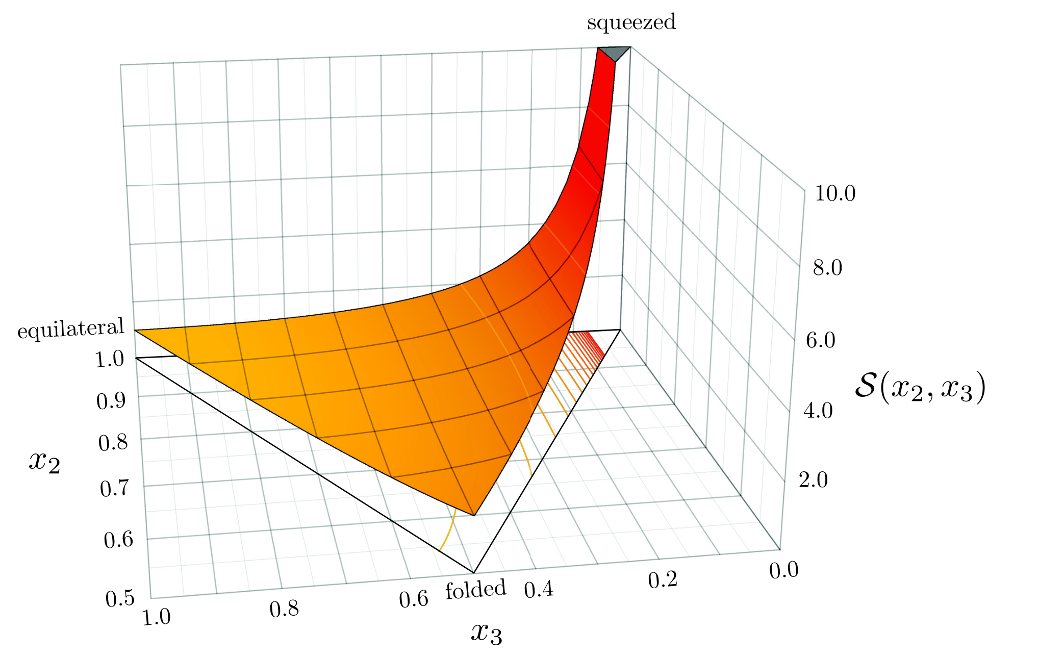
8.2 In-In Formalism

The problem of computing correlation functions in cosmology differs in important ways from the corresponding analysis of quantum field theory applied to particle physics.

In particle physics, the main observable is the $S$ -matrix, i.e. the transition probability for a state $|{in}\rangle$ in the far past to become some state $|{out}\rangle$ in the far future,

\langle{out}|\,S|{in}\rangle=\langle{out}(+{\infty})|{in}(-{\infty})\rangle\ .

(8.6)

The scattering particles are taken to be non-interacting at very early and very late times, when they are far from the interaction region, and the asymptotic states can be taken to be vacuum states of the free Hamiltonian $H_{0}$ .

Figure 24: Particle physicists compute in-out transition amplitudes.

In cosmology, on the other hand, the task is to determine the expectation values of products of operators at a fixed time. Boundary conditions are only imposed at very early times when their wavelengths are much smaller than the horizon and the interaction picture fields should have the same form as in Minkowski space. As we have seen in the previous section, this leads to the definition of the Bunch–Davies vacuum. In this section, we will describe the $in$ - $in$ formalism⁵⁵ 5 This is also referred to as the Schwinger–Keldysh formalism [47]. The use of the $in$ - $in$ formalism in cosmology was pioneered in [48, 49, 40, 42] (see also [50, 51]) and is reviewed in [43, 44]. to compute cosmological correlation functions as expectation values in two $|{in}\rangle$ states.

Figure 25: Cosmologists compute in-in expectation values.

Our goal is to compute $n$ -point functions of the curvature perturbation $\zeta$ or the gravitational wave polarization modes $\gamma^{\times}$ and $\gamma^{+}$ . We will collectively denote these fluctuations by the field $\psi=\{\zeta,\gamma^{\times},\gamma^{+}\}$ and consider expectation values of operators such as $\hat{Q}=\hat{\psi}_{{{\bf k}}_{1}}\hat{\psi}_{{{\bf k}}_{2}}\cdots\hat{\psi}_{{{\bf k}}_{n}}$ ,

\langle\hat{Q}(\tau)\rangle=\langle in|\,\hat{Q}(\tau)\,|in\rangle\,,

(8.7)

where $|in\rangle$ is the vacuum of the interacting theory at some moment ${\tau}_{i}$ in the far past, and $\tau>\tau_{i}$ is some later time, such as horizon crossing or the end of inflation. To compute the matrix element in (8.7) we evolve $Q(\tau)$ back to $\tau_{i}$ using the perturbed Hamiltonian $\delta H$ . Computing this time evolution is complicated by the interactions inside of $\delta H=H_{0}+H_{\rm int}$ , which lead to nonlinear equations of motion. We therefore introduce the interaction picture in which the leading time dependence of the fields is determined by the quadratic Hamiltonian $H_{0}$ (or linear equations of motion). Corrections arising from the interactions are then treated as a power series in $H_{\rm int}$ .

This leads to the following important result:

\framebox{$\displaystyle\langle\hat{Q}(\tau)\rangle\ =\ \langle 0|\ \bar{T}e^{i\int_{-\infty(1-i\epsilon)}^{\tau}\hat{H}_{\rm int}^{I}(\tau^{\prime})\,{\rm d}\tau^{\prime}}\,\hat{Q}^{I}(\tau)\ Te^{-i\int_{-\infty(1+i\epsilon)}^{\tau}\hat{H}_{\rm int}^{I}(\tau^{\prime\prime})\,{\rm d}\tau^{\prime\prime}}\,|0\rangle$}\ ,

(8.8)

where $T$ ( $\bar{T}$ ) is the (anti-)time-ordering symbol. Note that both $\hat{Q}^{I}$ and $\hat{H}_{\rm int}^{I}$ are evaluated using interaction picture operators. The standard $i\epsilon$ prescription has been used to effectively turn off the interaction in the far past and project the interacting $|in\rangle$ state onto the free vacuum $|0\rangle$ . By expanding the exponentials, we can compute the correlation function perturbatively in $\hat{H}_{\rm int}$ . For example, at leading order, we find

\framebox{$\displaystyle\langle\hat{Q}(\tau)\rangle\ =\ -i\int_{-\infty}^{\tau}{\rm d}\tau^{\prime}\ \langle 0|\,[\hat{Q}^{I}(\tau),\hat{H}_{\rm int}^{I}(\tau^{\prime})]\,|0\rangle$}\ .

(8.9)

We can use Feynman diagrams to organize the power series, drawing interaction vertices for every power of $\hat{H}_{\rm int}$ .

In the following insert, I will derive the $in$ - $in$ master formula (8.8). Readers who are more interested in applications of the result, may skip this part.

Derivation.—The time evolution of the operators in the Heisenberg picture is determined by

\frac{d\hat{\psi}}{d{\tau}}=i[\hat{H},\hat{\psi}]\,,\hskip 9.24994pt\frac{d\hat{p}_{\psi}}{d{\tau}}=i[\hat{H},\hat{p}_{\psi}]\,,

(8.10)

where $\hat{H}=\hat{H}_{0}+\hat{H}_{\rm int}$ is the perturbed Hamiltonian. This time evolution is complicated by the interactions inside $\hat{H}$ , which lead to nonlinear equations of motion. We therefore introduce the interaction picture in which the leading time dependence of the fields is determined by the quadratic Hamiltonian $\hat{H}_{0}$ (or, equivalently, by the linear equations of motion):

\frac{d\hat{\psi}^{I}}{d\tau}=i[\hat{H}_{0},\hat{\psi}^{I}]\ ,\hskip 9.24994pt\frac{d\hat{p}_{\psi}^{I}}{d\tau}=i[\hat{H}_{0},\hat{p}_{\psi}^{I}]\,.

(8.11)

The solution to these equations can be written as

\hat{\psi}^{I}_{{\bf k}}({\tau})=\psi^{I}_{k}({\tau})\,\hat{a}_{{\bf k}}+h.c.\,,

(8.12)

where $\psi^{I}_{k}({\tau})$ is the solution to the free-field equation and the operators $\hat{a}_{{\bf k}}$ define the free-field vacuum $|0\rangle$ . Corrections to the evolution of the operators can then be treated perturbatively in $\hat{H}_{\rm int}$ . Relatively straightforward algebraic manipulations of (8.10) and (8.11) allow us to express an operator in the Heisenberg picture in terms of operators in the interaction picture [42],

\hat{Q}({\tau})=\hat{F}^{-1}({\tau},{\tau}_{i})\,\hat{Q}^{I}({\tau})\,\hat{F}({\tau},{\tau}_{i})\,,

(8.13)

where

\hat{F}({\tau},{\tau}_{i})\equiv Te^{-i\int_{{\tau}_{i}}^{\tau}\hat{H}_{\rm int}^{I}({\tau}^{\prime\prime})\,{\rm d}{\tau}^{\prime\prime}}\,.

(8.14)

We can think of $\hat{F}({\tau},{\tau}_{i})$ as an operator evolving quantum states in the interaction picture,

|\Omega({\tau})\rangle=\hat{F}({\tau},{\tau}_{i})|\Omega({\tau}_{i})\rangle\,,

(8.15)

where $|\Omega({\tau}_{i})\rangle\equiv|\Omega\rangle$ . We would like to relate the vacuum of the interacting theory, $|\Omega\rangle$ , to the vacuum of the free theory, $|0\rangle$ . Inserting a complete set of energy eigenstates $\{|\Omega\rangle,|n\rangle\}$ of the full theory, where $|n\rangle$ are the excited states, we have

|0\rangle=|\Omega\rangle\langle\Omega|0\rangle+\sum_{n}|n\rangle\langle n|0\rangle\,,

(8.16)

and correspondingly

\displaystyle e^{-i\hat{H}({\tau}-{\tau}_{i})}|0\rangle

\displaystyle=e^{-i\hat{H}({\tau}-{\tau}_{i})}|\Omega\rangle\langle\Omega|0\rangle+\sum_{n}e^{-iE_{n}({\tau}-{\tau}_{i})}|n\rangle\langle n|0\rangle\,.

(8.17)

Adding a small imaginary part to the initial time, ${\tau}_{i}\to-{\infty}(1-i\epsilon)\equiv-{\infty}^{-}$ , will project out the excited states, $e^{-iE_{n}({\tau}-{\tau}_{i})}\to e^{-{\infty}\times\epsilon E_{n}}(\cdots)\to 0$ . We are then left with

\hat{F}({\tau},-{\infty}^{-})|\Omega\rangle=\frac{\hat{F}({\tau},-{\infty}^{-})|0\rangle}{\langle\Omega|0\rangle}\,.

(8.18)

The $i\epsilon$ prescription has effectively turned off the interactions in the far past and projected the interacting vacuum $|\Omega\rangle$ onto the free vacuum $|0\rangle$ . Setting $|\langle\Omega|0\rangle|\rightarrow 1$ , we arrive at the $in$ - $in$ master formula

\langle\hat{Q}({\tau})\rangle\ =\ \langle 0|\ \bar{T}e^{i\int_{-{\infty}^{+}}^{\tau}\hat{H}_{\rm int}^{I}({\tau}^{\prime})\,{\rm d}{\tau}^{\prime}}\,\hat{Q}^{I}({\tau})\ Te^{-i\int_{-{\infty}^{-}}^{\tau}\hat{H}_{\rm int}^{I}({\tau}^{\prime\prime})\,{\rm d}{\tau}^{\prime\prime}}\,|0\rangle\,,

(8.19)

where ${\infty}^{\pm}\equiv{\infty}(1{\pm}i\epsilon)$ . The integration contour goes from $-{\infty}(1-i\epsilon)$ to ${\tau}$ (where the correlation function is evaluated) and back to $-{\infty}(1+i\epsilon)$ .

8.3 Gravitational Floor

Let us now apply this formalism to the calculation of the bispectrum of curvature perturbations in single-field slow-roll inflation [40]. The nonlinearities of the gravitational evolution produce a minimal amount of non-Gaussianity which we will call the “gravitational floor”. Unfortunately, the amplitude of the signal is too small to be detectable in the foreseeable future.

To compute the bispectrum we need to expand the inflationary action (7.41) to third order in perturbations. It is convenient to perform the computation in comoving gauge, cf. eqs. (7.52) and (7.53). In §7.1.2, we solved the lapse $N$ and the shift $N_{i}$ to first order in $\zeta$ . This is sufficient also for the cubic action since second-order and third-order perturbations in $N$ and $N_{i}$ will multiply the first-order and zeroth-order constraint equation, respectively. Substituting (7.54) into (7.41) and expanding to third order, we find [40]

	$\displaystyle S_{3}$	$\displaystyle=\frac{1}{2}\int{\rm d}t\,{\rm d}^{3}x\,a^{3}\Big(2\varepsilon^{2}\,\zeta(\zeta^{\prime})^{2}-4a^{-2}\varepsilon^{2}\,\zeta^{\prime}(\partial\zeta)(\partial\zeta)+2a^{-2}\varepsilon^{2}\,\zeta(\partial\zeta)^{2}$
		$\displaystyle\hskip 85.35826pt+a^{-2}\varepsilon\eta^{\prime}\,\zeta^{2}\zeta^{\prime}+a^{-2}\varepsilon\,\partial\zeta\partial\beta\partial^{2}\beta+\frac{1}{2}a^{-2}\varepsilon\,\partial^{2}\zeta(\partial\beta)^{2}+2f(\zeta)\frac{\delta L_{2}}{\delta\zeta}\Big)\,,$		(8.20)

where we have defined

	$\displaystyle\frac{\delta L_{2}}{\delta\zeta}$	$\displaystyle\equiv(a^{3}\varepsilon\,\zeta^{\prime})^{\prime}-a\varepsilon\partial^{2}\zeta\,,$		(8.21)
	$\displaystyle f(\zeta)$	$\displaystyle\equiv\frac{\eta}{4}\zeta^{2}+\frac{\zeta\zeta^{\prime}}{H}+\frac{-(\partial\zeta)^{2}+\partial^{-2}(\partial_{i}\partial_{j}(\partial_{i}\zeta\partial_{j}\zeta))}{4a^{2}H^{2}}+\frac{\partial\zeta\partial\beta-\partial^{-2}(\partial_{i}\partial_{j}(\partial_{i}\zeta\partial_{j}\beta))}{2a^{2}H^{2}}\,.$		(8.22)

Maldacena showed that the term proportional to $f(\zeta)$ in (8.20) can be removed by a field redefinition,

\zeta\to\tilde{\zeta}+f(\tilde{\zeta})\,.

(8.23)

This field redefinition has the following effect on the correlation function:

\langle\zeta({\bf x}_{1})\zeta({\bf x}_{2})\zeta({\bf x}_{3})\rangle=\langle\tilde{\zeta}({\bf x}_{1})\tilde{\zeta}({\bf x}_{2})\tilde{\zeta}({\bf x}_{3})\rangle+\frac{\eta}{2}\left(\langle\tilde{\zeta}({\bf x}_{1})\tilde{\zeta}({\bf x}_{2})\rangle\langle\tilde{\zeta}({\bf x}_{1})\tilde{\zeta}({\bf x}_{3})\rangle+{\rm cyclic}\right)+\cdots\,.

(8.24)

The term proportional to $f(\zeta)$ in (8.20) therefore leads to a contribution to $f_{\rm NL}$ of order $\eta\ll 1$ . The effect of the remaining interactions is computed by expanding the $in$ - $in$ master formula (8.8) to first order in $H_{\rm int}=-L_{3}+{\cal O}(\zeta^{4})$ ,

\langle\zeta_{{\bf k}_{1}}\zeta_{{\bf k}_{2}}\zeta_{{\bf k}_{3}}\rangle=-i\int_{-\infty}^{0}{\rm d}\tau\ \langle 0|\big[\hat{\zeta}_{{\bf k}_{1}}\hat{\zeta}_{{\bf k}_{2}}\hat{\zeta}_{{\bf k}_{3}}(0),\hat{H}_{\rm int}(\tau)\big]|0\rangle\,,

(8.25)

where we have switched to conformal time and taken the superhorizon limit $k\tau\to 0$ .

Back-of-the-envelope estimate.—Before embarking on a lengthy calculation of the bispectrum, it is often advisable to perform an order-of-magnitude estimate of the expected size of the signal, i.e. to estimate (8.25) without explicitly performing the integral. For example, the first term in (8.20), can be written as

\int{\rm d}\tau\,H_{\rm int}(\tau)\subset-\int{\rm d}\tau{\rm d}^{3}x\,a^{2}\varepsilon^{2}\zeta\dot{\zeta}^{2}\ .

(8.26)

We only need to keep track of factors of $H$ and $\varepsilon$ . Any time- and momentum-dependence will work itself out and only contributes to the shape function. Using $a\propto H^{-1}$ and $\zeta\propto\dot{\zeta}\propto{\cal P}_{\zeta}^{1/2}\sim H/\sqrt{\varepsilon}$ , we estimate that the contribution from the three-point vertex is $\sim H\sqrt{\varepsilon}$ . Combining this with estimates for the size of the three external legs, $\zeta^{3}\sim H^{3}\varepsilon^{-3/2}$ , we find

\langle\zeta^{3}\rangle=-i\int{\rm d}\tau\,\langle[\hat{\zeta}^{3},\hat{H}_{\rm int}(\tau)]\rangle\propto\frac{H^{4}}{\varepsilon}\propto{\cal O}(\varepsilon)\,{\cal P}_{\zeta}^{2}\sim f_{\rm NL}\,{\cal P}_{\zeta}^{2}\ .

(8.27)

Similar results are obtained for the other interactions in (8.20), $f_{\rm NL}\sim{\cal O}(\varepsilon)$ . We also include the contribution from the field redefinition in (8.24), $f_{\rm NL}\sim{\cal O}(\eta)$ . We conclude that the non-Gaussianity in slow-roll inflation is slow-roll suppressed,

f_{\rm NL}\sim{\cal O}(\varepsilon,\eta)\ll 1\,.

(8.28)

This small amount of non-Gaussianity will be unobservable in the CMB.

To get the full momentum-dependence of the bispectrum, we actually have to do some real work and compute the integral in (8.25) using the free-field mode functions for $\zeta$ . The final result for the dimensionless bispectrum is [40]

	$\displaystyle\frac{{\cal B}_{\zeta}(k_{1},k_{2},k_{3})}{{\cal P}_{\zeta}^{2}}$	$\displaystyle\,=\,\frac{\varepsilon}{2}\left[-\left(\frac{k_{1}^{2}}{k_{2}k_{3}}+2\,{\rm perms.}\right)+\left(\frac{k_{1}}{k_{2}}+5\,{\rm perms.}\right)+\frac{8}{k_{t}}\left(\frac{k_{1}k_{2}}{k_{3}}+2\,{\rm perms.}\right)\right]$
		$\displaystyle\hskip 17.07182pt+\frac{\eta}{2}\left(\frac{k_{1}^{2}}{k_{2}k_{3}}+2\,{\rm perms.}\right)\,,$		(8.29)

where $k_{t}\equiv k_{1}+k_{2}+k_{3}$ . It is interesting to take the squeezed limit, $k_{3}\ll k_{1}\approx k_{2}$ , of the result:

\lim_{k_{3}\to 0}\frac{{\cal B}_{\zeta}(k_{1},k_{2},k_{3})}{{\cal P}_{\zeta}^{2}}=(2\varepsilon+\eta)\,\frac{k_{1}}{k_{3}}\,.

(8.30)

Note that the coefficient in the squeezed limit equals the deviation from scale invariance of the power spectrum, $1-n_{\rm s}=2\varepsilon+\eta$ . In fact, this is a general result that applies to all models of single-field inflation, not necessarily just to slow-roll models. The single-field consistency relation states that [40, 52]

\boxed{\lim_{k_{3}\to 0}B_{\zeta}(k_{1},k_{2},k_{3})=(1-n_{\rm s})\,P_{\zeta}(k_{1})P_{\zeta}(k_{3})}\ ,

(8.31)

i.e. the squeezed limit of the three-point function is suppressed by $(1-n_{\rm s})$ and vanishes for perfectly scale-invariant perturbations.

Proof.—The squeezed triangle correlates one long-wavelength mode, $k_{\rm L}=k_{3}$ , to two short-wavelength modes, $k_{\rm S}=k_{1}\approx k_{2}$ ,

\langle\zeta_{{\bf k}_{1}}\zeta_{{\bf k}_{2}}\zeta_{{\bf k}_{3}}\rangle\ \to\ \langle(\zeta_{{\bf k}_{\rm S}})^{2}\zeta_{{\bf k}_{\rm L}}\rangle\,.

(8.32)

Modes with longer wavelengths freeze earlier. The long mode $\zeta_{{\bf k}_{\rm L}}$ will therefore already be frozen and act as a classical background wave when the two short modes $\zeta_{{\bf k}_{\rm S}}$ exit the horizon. This provides an intuitive way to study the correlations between long and short modes.

Why should $(\zeta_{{\bf k}_{\rm S}})^{2}$ be correlated with $\zeta_{{\bf k}_{\rm L}}$ ? The theorem says that it isn’t correlated if $\zeta_{\bf k}$ is precisely scale-invariant, but that the short scale power does get modified by the long-wavelength mode if $n_{\rm s}\neq 1$ . Let’s see why. We decompose the evaluation of (8.32) into two steps:

i)

we calculate the power spectrum of short fluctuations $\langle\zeta_{{\rm S}}^{2}\rangle_{\zeta_{{\rm L}}}$ in the presence of a long mode $\zeta_{{\rm L}}$ ;
ii)

we then calculate the correlation $\langle(\zeta_{{\rm S}})^{2}\zeta_{{\rm L}}\rangle$ , i.e. average the short-scale power spectrum over realizations of the long modes.

The calculation of $\langle\zeta_{{\rm S}}^{2}\rangle_{\zeta_{{\rm L}}}$ is simplest in real space: When the background mode is homogeneous, $\zeta_{\rm L}(x)\equiv\bar{\zeta}_{\rm L}$ , it can be reabsorbed simply by a rescaling of the spatial coordinates, $\tilde{x}^{i}=e^{\bar{\zeta}_{\rm L}}x^{i}$ (recall that ${\rm d}s^{2}=-{\rm d}t^{2}+a^{2}(t)e^{2\zeta({\bf x},t)}{\rm d}{\bf x}^{2}$ ). After this rescaling, $\bar{\zeta}_{\rm L}$ no longer appears in the action, so that the two-point function in the new coordinates is the same as in the absence of $\bar{\zeta}_{\rm L}$ . In other words, in the limit of constant $\bar{\zeta}_{\rm L}$ , we have

\langle\zeta_{\rm S}({\bf x}_{1})\zeta_{\rm S}({\bf x}_{2})\rangle_{\bar{\zeta}_{\rm L}}=\langle\zeta_{\rm S}(\tilde{\bf x}_{1})\zeta_{\rm S}(\tilde{\bf x}_{2})\rangle\,.

(8.33)

When $\zeta_{\rm L}$ is slowly varying, we can evaluate it at the middle point ${\bf x}_{+}\equiv\frac{1}{2}({\bf x}_{1}+{\bf x}_{2})$ to get

\tilde{\bf x}_{-}\simeq{\bf x}_{-}+\zeta_{\rm L}({\bf x}_{+})\cdot{\bf x}_{-}+\cdots\,,

(8.34)

where we defined ${\bf x}_{-}\equiv{\bf x}_{1}-{\bf x}_{2}$ . The two-point function at linear order in $\zeta_{\rm L}$ therefore is

\langle\zeta_{\rm S}({\bf x}_{2})\zeta_{\rm S}({\bf x}_{3})\rangle_{\zeta_{\rm L}(x)}\simeq\xi_{\rm S}(|{\bf x}_{-}|)+\zeta_{\rm L}({\bf x}_{+})[{\bf x}_{-}\cdot\nabla\xi_{\rm S}(|{\bf x}_{-}|)]\ ,

(8.35)

where

\xi_{\rm S}(|{\bf x}_{-}|)\equiv\int\frac{{\rm d}^{3}k_{\rm S}}{(2\pi)^{3}}\,P_{\zeta}(k_{\rm S})\,e^{i{\bf k}_{\rm S}\cdot{\bf x}_{-}}\,.

(8.36)

The three-point function then is

	$\displaystyle\langle\zeta_{\rm S}({\bf x}_{1})\zeta_{\rm S}({\bf x}_{2})\zeta_{\rm L}({\bf x}_{3})\rangle$	$\displaystyle\ \simeq\ \langle\zeta_{\rm L}({\bf x}_{3})\zeta_{\rm L}({\bf x}_{+})\rangle[{\bf x}_{-}\cdot\nabla\xi_{\rm S}(\|{\bf x}_{-}\|)]\,,$
		$\displaystyle\ =\ \int\frac{{\rm d}^{3}k_{\rm L}}{(2\pi)^{3}}\int\frac{{\rm d}^{3}k_{\rm S}}{(2\pi)^{3}}\,e^{i{\bf k}_{\rm L}\cdot({\bf{x}}_{3}-{\bf{x}}_{+})}P_{\zeta}(k_{\rm L})P_{\zeta}(k_{\rm S})\left[{\bf k}_{\rm S}\cdot\frac{\partial}{\partial{\bf k}_{\rm S}}\right]e^{i{\bf k}_{\rm S}\cdot{\bf x}_{-}}\,.$		(8.37)

Integrating by parts, inserting $1=\int{\rm d}^{3}k_{3}\,\delta_{D}({\bf k}_{3}+{\bf k}_{\rm L})$ and using

\frac{\partial}{\partial{\bf k}_{\rm S}}\cdot[{\bf k}_{\rm S}P_{\zeta}(k_{\rm S})]=P_{\zeta}(k_{\rm S})\,\frac{d\ln(k_{\rm S}^{3}P_{\zeta}(k_{\rm S}))}{d\ln k_{\rm S}}\,,

(8.38)

we get

	$\displaystyle\langle\zeta_{\rm S}({\bf x}_{1})\zeta_{\rm S}({\bf x}_{2})\zeta_{\rm L}({\bf x}_{3})\rangle$	$\displaystyle=-\int\frac{{\rm d}^{3}k_{3}}{(2\pi)^{3}}\int\frac{{\rm d}^{3}k_{\rm L}}{(2\pi)^{3}}\int\frac{{\rm d}^{3}k_{\rm S}}{(2\pi)^{3}}\ e^{-i{\bf k}_{1}\cdot{\bf x}_{1}-i{\bf k}_{\rm L}\cdot{\bf x}_{+}+i{\bf k}_{\rm S}\cdot{\bf x}_{-}}$
		$\displaystyle\hskip 28.45274pt\times\left[(2\pi)^{3}\delta_{D}({\bf k}_{1}+{\bf k}_{\rm L})P_{\zeta}(k_{1})P_{\zeta}(k_{\rm S})\,\frac{d\ln(k_{\rm S}^{3}P_{\zeta}(k_{\rm S}))}{d\ln k_{\rm S}}\right].$		(8.39)

Letting ${\bf k}_{\rm L}={\bf k}_{2}+{\bf k}_{3}$ and ${\bf k}_{\rm S}=\frac{1}{2}({\bf k}_{2}-{\bf k}_{3})$ , we get $-i{\bf k}_{\rm L}\cdot{\bf x}_{+}+i{\bf k}_{\rm S}\cdot{\bf x}_{-}=-i{\bf k}_{2}\cdot{\bf x}_{2}-i{\bf k}_{3}\cdot{\bf x}_{3}$ . Changing variables in the integration and Fourier transforming, we get

	$\displaystyle\lim_{k_{3}\to 0}\langle\zeta_{{\bf k}_{1}}\zeta_{{\bf k}_{2}}\zeta_{{\bf k}_{3}}\rangle$	$\displaystyle\ =\ -(2\pi)^{3}\delta_{D}({\bf k}_{1}+{\bf k}_{2}+{\bf k}_{3})\,P_{\zeta}(k_{1})P_{\zeta}(k_{3})\,\frac{d\ln k_{3}^{3}P_{\zeta}(k_{3})}{d\ln k_{3}}\,,$
		$\displaystyle\ =\ (2\pi)^{3}\delta_{D}({\bf k}_{1}+{\bf k}_{2}+{\bf k}_{3})\,(1-n_{\rm s})\,P_{\zeta}(k_{1})P_{\zeta}(k_{3})\,.$		(8.40)

This completes the proof.

The fact that the squeezed limit of the bispectrum for single-field inflation vanished implies that it can be used as a clean diagnostic for extra fields during inflation. In the next section, we will expand on this view of the squeezed limit as a particle detector.

9 Heavy Relics

As we have seen in the previous sections, computing the quantum correlations in single-field slow-roll inflation is a well-defined problem leading to clean predictions for the cosmological correlation functions. In this final section, we will look for deviations from those predictions associated with the existence of extra particles during inflation.

We will begin, in §9.1, with a review of the allowed spectrum of particles in de Sitter space, highlighting the qualitative differences to the corresponding results in flat space. In §9.2 and §9.3, we derive the basic observational imprints that these massive fields create when they are excited during inflation. For further details we refer the reader to the vast literature on the subject, e.g. [53, 54, 55, 56, 57, 38, 58, 59, 60, 61, 62, 63].

9.1 Massive Fields in de Sitter

Particles in Minkowski space are classified as unitary irreducible representations of the Poincaré group [64, 65]. The eigenvalues of the Casimir operators of the Poincaré group are related as follows to the mass $m$ and the spin $s$ of the particles:

	$\displaystyle{\cal C}_{1}$	$\displaystyle\equiv P_{\mu}P^{\mu}=m^{2}\,,$		(9.1)
	$\displaystyle{\cal C}_{2}$	$\displaystyle\equiv W_{\mu}W^{\mu}=-s(s+1)\hskip 1.0ptm^{2}\,,$		(9.2)

where $P_{\mu}$ is the four-momentum and $W_{\mu}$ is the Pauli-Lubanski pseudovector. We distinguish between massive and massless particles. Massive particles carry $2s+1$ degrees of freedom (transverse and longitudinal polarizations), while massless particles have only two transverse polarizations.

Similarly, particles in de Sitter space are classified as unitary irreducible representations of the de Sitter group $SO(1,4)$ . The Casimir operators of the de Sitter group have the following eigenvalues [66, 67]:

	$\displaystyle{\cal C}_{1}$	$\displaystyle\equiv\frac{1}{2}M_{AB}M^{AB}=m^{2}-2(s-1)(s+1)H^{2}\,,$		(9.3)
	$\displaystyle{\cal C}_{2}$	$\displaystyle\equiv W_{A}W^{A}=-s(s+1)\left[m^{2}-\left(s^{2}+s-\frac{1}{2}\right)H^{2}\right],$		(9.4)

where $M_{AB}$ are the generators of $SO(1,4)$ , with $A,B=\{0,\ldots,4\}$ . Notice that this time the Casimir (9.3) is not just proportional to the mass alone, but also has a term that depends on spin. For $s\geq 1$ , the representations of de Sitter space fall into three distinct categories [68, 69, 70]:

principal series	complementary series	discrete series
$\displaystyle\frac{m^{2}}{H^{2}}\geq\left(s-\frac{1}{2}\right)^{2}$	$\displaystyle s(s-1)<\frac{m^{2}}{H^{2}}<\left(s-\frac{1}{2}\right)^{2}$	$\displaystyle\frac{m^{2}}{H^{2}}=s(s-1)-t(t+1)$ ,

for $t=0,1,2,...,s\!-\!1$ , which is called the depth of the field. Masses that are not associated with one of the above categories correspond to non-unitary representations and are therefore not allowed in the spectrum (see Fig. 26). At the specific mass values corresponding to the discrete series, the system gains an additional gauge invariance and some of the lowest helicity modes become pure gauge modes; this phenomenon is called partial masslessness [71]. We see that unitarity demands the existence of a lower bound

\displaystyle m^{2}\geq s(s-1)H^{2}\,,

(9.5)

on the masses of fields except those that belong to the discrete series. For $s=2$ , this is known as the Higuchi bound [72].

Figure 26: Spectrum of spin-0 (top) and spin-4 fields (bottom) in de Sitter space. The green points correspond to masses in the discrete series.

The Lagrangian for massive fields with arbitrary spin in flat space was constructed by Singh and Hagen in [73, 74], and generalized to (A)dS spaces in [75]. For massive fields with spin greater than 2, the action is rather complex and requires introducing auxiliary fields of lower spins. An alternative, which we will follow, is to use a group theoretical approach to find the equations of motion directly [66]. In four spacetime dimensions, a massive bosonic spin- $s$ field is described by a totally symmetric rank- $s$ tensor, $\sigma_{\mu_{1}\cdots\mu_{s}}$ , subject to the constraints

\displaystyle\nabla^{\mu_{1}}\sigma_{\mu_{1}\cdots\mu_{s}}=0\,,\quad{\sigma^{\mu}}_{\mu\mu_{3}\cdots\mu_{s}}=0\,.

(9.6)

The conditions in (9.6) project out the components of the tensor which transform as fields with lower spins. The Casimir eigenvalue equation of the de Sitter group then gives the on-shell wave equation satisfied by these fields:

\displaystyle\big(\Box-m_{s}^{2}\big)\sigma_{\mu_{1}\cdots\mu_{s}}=0\,,

(9.7)

where $\Box\equiv\nabla_{\mu}\nabla^{\mu}$ is the Laplace-Beltrami operator on ${\rm dS}_{4}$ and $m_{s}^{2}\equiv m^{2}-(s^{2}-2s-2)H^{2}$ . The shift in the mass arises from the mismatch between the Casimir and Laplace-Beltrami operators in de Sitter space and is necessary to describe the correct representations for massless fields. Explicit solutions to the equation of motion (9.7) can be found in Appendix A of [59]. The spatial components contain all the physical degrees of freedom, while the other components are constrained variables or pure gauge modes.⁶⁶ 6 This can be seen by solving the equation of motion (9.7) explicitly, where the normalizations of non-physical components become singular [59]. The late-time behaviour of the solution is

\lim_{\tau\to 0}\sigma_{i_{1}\cdots i_{s}}(\tau,{\bf{x}})=\sum_{\pm}\tau^{\Delta_{\pm}-s}{\sigma}^{\pm}_{i_{1}\cdots i_{s}}({\bf{x}})\,,

(9.8)

where $\Delta_{\pm}$ is the conformal dimension of the field

\Delta_{\pm}=\frac{3}{2}\pm i\mu\,,\quad\mu\equiv\sqrt{\frac{m^{2}}{H^{2}}-\left(s-\frac{1}{2}\right)^{2}}\,.

(9.9)

Note that, for $s=0$ , the value $m=0$ corresponds to a conformally-coupled scalar field. In the limit $m\gg sH$ , the parameter $\mu$ becomes the mass of the particle in Hubble units, $\mu\to m/H$ . Particles belonging to the principal series correspond to $\mu\geq 0$ , which covers the largest mass range. For real $\mu$ , the asymptotic scaling is given by a complex-conjugate pair, resulting in a wavefunction that oscillates logarithmically in conformal time. The complementary series has imaginary $\mu$ and corresponds to the interval $-i\mu=(0,1/2)$ . In that case, only the growing mode survives in the late-time limit.

Figure 27: Superhorizon evolution of a massive scalar field. The decay of the field amplitude is determined by the mass of the field.

9.2 Local and Non-Local

In the remainder of this section, we will study the imprints of massive particles on inflationary correlations functions. Massive particles during inflation can have two types of effects:

•

Particles with masses $M\gg H$ can be integrated out, leading to an EFT of inflaton interactions:

These local interactions create characteristic imprints in the non-Gaussianity of the inflaton fluctuations. In particular, the soft limits of the resulting correlation functions must satisfy the single-field consistency relation discussed in the previous section.
•

Particles with masses $M\lesssim{\rm few}\times H$ cannot be integrated out completely, but are produced nonperturbatively by the expanding spacetime. When these particles decay, they produce characteristic non-local signatures in cosmological correlators. The single-field consistency relation will be violated.

Local effects

To illustrate the local effects arising from massive particles, we consider the following two-field example:

{\cal L}\,=\,-\frac{1}{2}(\partial_{\mu}\phi)^{2}-V(\phi)-\frac{1}{2}(\partial_{\mu}\sigma)^{2}-\frac{1}{2}M^{2}\sigma^{2}+\frac{\sigma(\partial_{\mu}\phi)^{2}}{\tilde{\Lambda}}\,,

(9.10)

where $M\gg H$ . Integrating out the massive field $\sigma$ gives

	$\displaystyle{\cal L}_{\rm eff}$	$\displaystyle\,=\,-\frac{1}{2}(\partial_{\mu}\phi)^{2}-V(\phi)+\frac{1}{8\tilde{\Lambda}^{2}}(\partial_{\mu}\phi)^{2}\,\frac{1}{\Box+M^{2}}\,(\partial_{\mu}\phi)^{2}+\cdots$
		$\displaystyle\,=\,-\frac{1}{2}(\partial_{\mu}\phi)^{2}-V(\phi)+\frac{1}{8\tilde{\Lambda}^{2}M^{2}}\left((\partial_{\mu}\phi)^{4}+(\partial_{\mu}\phi)^{2}\,\frac{\Box}{M^{2}}\,(\partial_{\mu}\phi)^{2}+\cdots\right),$		(9.11)

where the second line is written as an expansion in $(H/M)^{2}$ , with $H$ being the Hubble scale during inflation. Truncating the expansion of EFT operators at the lowest order, we obtain the Lagrangian [76]

{\cal L}_{\rm eff}={\cal L}_{0}(\phi)+\frac{(\partial_{\mu}\phi)^{4}}{8\Lambda^{4}}\,,

(9.12)

where ${\cal L}_{0}$ is the canonical slow-roll Lagrangian and $\Lambda^{2}\equiv\tilde{\Lambda}M$ . Following [76], we will compute the bispectrum induced by the interaction in (9.12).

This time it is useful to work in spatially flat gauge. At leading order in the slow-roll parameters, the action for the inflaton perturbation $\varphi\equiv\phi-\bar{\phi}(t)$ can then be calculated from (9.12) without including the contributions from $\sqrt{-g}R$ . The intuitive reason for this simplification is that in the limit of a flat potential the perturbation $\varphi$ does not induce a perturbation in the spacetime curvature. Evaluating one of the legs of the interaction $(\partial_{\mu}\phi)^{4}$ on the background solution, we get

\parbox[c]{108.405pt}{\includegraphics[scale={.5}]{Figures/3point2}}\qquad\Leftrightarrow\qquad{\cal L}_{{\rm eff},3}=-\frac{\phi^{\hskip 1.0pt\prime}}{4\Lambda^{4}}\,\varphi^{\prime}(\partial_{\mu}\varphi)^{2}\,.

(9.13)

Using this interaction, we can compute the bispectrum $\langle\varphi\varphi\varphi\rangle$ . We will relate the result to $\langle\zeta\zeta\zeta\rangle$ at horizon crossing to avoid the error that would be induced by the superhorizon evolution of $\varphi$ . To perform this matching, we, in principle, need to know the relation between $\varphi$ and $\zeta$ up to second order. However, the quadratic term is slow-roll suppressed, so it suffices to use the linear relationship

\zeta=-\frac{H}{\phi^{\hskip 1.0pt\prime}}\,\varphi\,.

(9.14)

Feeding ${\cal H}_{\rm int}=-{\cal L}_{{\rm eff},3}$ into the $in$ - $in$ master formula (8.19), we find

$\displaystyle\frac{{\cal B}_{\zeta}(k_{1},k_{2},k_{3})}{{\cal P}_{\zeta}^{2}}$	$\displaystyle\,=\,-\frac{4i}{k_{1}k_{2}k_{3}}\,\frac{(\phi^{\prime})^{2}}{\Lambda^{4}}\int_{-\infty}^{0}{\rm d}\tau\left(-k_{1}^{2}k_{2}^{2}k_{3}^{3}\,\tau^{2}-({\bf k}_{1}\cdot{\bf k}_{2})k_{3}^{2}(1-ik_{1}\tau)(1-ik_{2}\tau)\right)e^{ik_{t}\tau}$
	$\displaystyle\qquad+{\rm perms.}+c.c.\,,$	(9.15)
	$\displaystyle\hskip 153.6447pt\uparrow\hskip 85.35826pt\uparrow$
	$\displaystyle\hskip 147.95424pt{(\varphi^{\prime})^{3}}\hskip 56.9055pt(\varphi^{\prime})(\partial_{i}\varphi)^{2}$

where $k_{t}\equiv k_{1}+k_{2}+k_{3}$ . Evaluating the integral, we get [76]

\frac{{\cal B}_{\zeta}(k_{1},k_{2},k_{3})}{{\cal P}_{\zeta}^{2}}=\frac{8}{k_{1}k_{2}k_{3}}\frac{(\phi^{\prime})^{2}}{\Lambda^{4}}\,\frac{1}{k_{t}^{2}}\Bigg(\sum_{i}k_{i}^{5}+\sum_{i\neq j}(2k_{i}^{4}k_{j}-3k_{i}^{3}k_{j}^{2})+\sum_{i\neq j\neq l}(k_{i}^{3}k_{j}k_{l}-4k_{i}^{2}k_{j}^{2}k_{l})\Bigg)\,.

(9.16)

The following features of this result are worth noting:

•

The signal peaks in the equilateral configuration (cf. Fig. 23).
•

The squeezed limit, $\lim_{k_{\rm L}\to 0}\langle\zeta_{{\bf k}_{\rm S}}\zeta_{{\bf k}_{\rm S}}\zeta_{{\bf k}_{\rm L}}\rangle$ , is an analytic function of $k_{\rm L}/k_{\rm S}$ . This is a consequence of the interaction being local.
•

The amplitude is bounded,

$f_{\rm NL}=\frac{35}{108}\frac{(\phi^{\prime})^{2}}{\Lambda^{4}}<1\,,$ (9.17)

where the final inequality follows from $\phi^{\prime}<\Lambda^{2}$ , as required by consistency of the truncation used in (9.12).

Nonlocal effects

For $M\lesssim{\rm few}\times H$ , there are effects of massive particles that cannot be captured by local inflaton interactions, i.e. the field cannot be integrated out completely. The non-locality of the effective inflaton interactions will be reflected in a characteristic non-analyticity in its correlation functions.

As a concrete example, we consider a massive scalar field $\sigma$ . Its two-point function in de Sitter space is

\displaystyle\langle\sigma_{\bf k}(\tau)\sigma_{{\bf k}^{\prime}}(\tau^{\prime})\rangle^{\prime}=\frac{\pi}{4}H^{2}(\tau\tau^{\prime})^{3/2}e^{-\pi\mu}H_{i\mu}(-k\tau)H^{*}_{i\mu}(-k\tau^{\prime})\,,

(9.18)

where $H_{i\mu}\equiv H_{i\mu}^{(1)}$ is the Hankel function of the first kind and $\mu\equiv\sqrt{m^{2}/H^{2}-9/4}$ . For now, let us focus on particles belonging to the principal series, so that $\mu$ is real. The local part of the two-point function has support only at coincident points in position space, while the non-local part describes correlations over long distances. In Fourier space, the local and non-local parts of the two-point function are analytic and non-analytic in the momentum $k$ , respectively. In the late-time limit, we can split (9.18) into its local and non-local parts

	$\displaystyle\lim_{\tau,\tau^{\prime}\to 0}\langle\sigma_{\bf k}(\eta)\sigma_{{\bf k}^{\prime}}(\tau^{\prime})\rangle^{\prime}_{\rm local}$	$\displaystyle=\frac{H^{2}(\tau\tau^{\prime})^{3/2}}{4\pi}\Gamma(-i\mu)\Gamma(i\mu)\left[e^{\pi\mu}\Big(\frac{\tau}{\tau^{\prime}}\Big)^{i\mu}+e^{-\pi\mu}\Big(\frac{\tau}{\tau^{\prime}}\Big)^{-i\mu}\right],$		(9.19)
	$\displaystyle\lim_{\tau,\tau^{\prime}\to 0}\langle\sigma_{\bf k}(\tau)\sigma_{{\bf k}^{\prime}}(\tau^{\prime})\rangle^{\prime}_{\text{non-local}}$	$\displaystyle=\frac{H^{2}(\tau\tau^{\prime})^{3/2}}{4\pi}\left[\Gamma(-i\mu)^{2}\Big(\frac{k^{2}\tau\tau^{\prime}}{4}\Big)^{i\mu}+\Gamma(i\mu)^{2}\Big(\frac{k^{2}\tau\tau^{\prime}}{4}\Big)^{-i\mu}\right].$		(9.20)

Note that $\Gamma(\pm i\mu)\to e^{-\pi\mu/2}$ for large $\mu$ , resulting in an overall suppression of $e^{-\pi\mu}$ of the non-local contribution (9.20). In the next section, we will see how the non-analyticity of the non-local part of the two-point function of $\sigma$ is reflected in the inflationary correlators.

9.3 Cosmological Collider Physics

The correlations in the massive field $\sigma$ become observable when they get converted to inflaton fluctuations through interactions such as the mixing term in (9.10):

{\cal L}\,\supset\,\frac{\sigma(\partial_{\mu}\phi)^{2}}{\Lambda}\,.

(9.21)

Evaluating one of the legs of the inflaton field on the background solution, $\bar{\phi}$ , leads to a bispectrum for the inflaton fluctuations $\varphi$ (and hence of the curvature perturbations $\zeta$ ); cf. Fig. 28. The derivation of the bispectrum of curvature perturbations can be found in [58, 59]. Here, we summarize the main features of the result:

Figure 28: The spontaneous creation and decay of a massive particle

\sigma

produces a four-point function for the inflaton field

\phi

. Evaluating one of the legs on the background solution,

\bar{\phi}

, leads to a three-point function for the inflaton fluctuations

\varphi

•

The non-local effect associated with the massive particle exchange shows up as a non-analyticity in the squeezed limit, $\lim_{k_{\rm L}\to 0}\langle\zeta_{{\bf k}_{\rm S}}\zeta_{-{\bf k}_{\rm S}}\zeta_{{\bf k}_{\rm L}}\rangle$ . Between the horizon crossing times of the long mode $\zeta_{\rm L}$ and the short modes $\zeta_{\rm S}$ the amplitude of the massive field oscillates with a frequency set by the mass of the field. This leads to distinct oscillations in the bispectrum of curvature perturbations:

\lim_{k_{\rm L}\to 0}\langle\zeta_{{\bf k}_{\rm S}}\zeta_{-{\bf k}_{\rm S}}\zeta_{{\bf k}_{\rm L}}\rangle\,\propto\,\left(\frac{k_{\rm L}}{k_{\rm S}}\right)^{3/2}\cos\left[\frac{M}{H}\ln\left(\frac{k_{\rm L}}{k_{\rm S}}\right)+\delta\right],

(9.22)

where $\delta$ is a computable phase [58]. We see that the mass $M$ of the field is encoded in the frequency of the oscillations (see Fig. 29).

•

Particles with spin $s$ lead to a unique angular dependence (see Fig. 30):

\lim_{k_{\rm L}\to 0}\langle\zeta_{{\bf k}_{\rm S}}\zeta_{-{\bf k}_{\rm S}}\zeta_{{\bf k}_{\rm L}}\rangle\,\propto\,P_{s}(\cos\theta)\,,

(9.23)

where $\cos\theta\equiv{\bf k}_{\rm S}\cdot{\bf k}_{\rm L}$ and $P_{s}$ is a Legendre polynomial of degree $s$ .

Figure 29: Shape function for the bispectrum arising from the exchange of a spin-2 particle with

\mu=5

, evaluated in the isosceles-triangle configuration,

x_{2}\equiv k_{2}/k_{1}=1

(figure adapted from [59]). The dotted line is the non-local part of the signal.

Figure 30: Shape function for the bispectrum arising from the exchange of a spin-2 particle with

\mu=5

, as a function of the base angle

\theta=\cos^{-1}(\hat{\bf k}_{1}\cdot\hat{\bf k}_{3})

for fixed ratios of

x_{3}\equiv k_{3}/k_{1}

(figure adapted from [59]).

There are several effects that determine the amplitude of the signal:

•

If we make the conservative assumption that the interaction in (9.21) is only of gravitational strength [58], then the scale determining the mixing between $\sigma$ and $\phi$ is $\Lambda=M_{\rm pl}$ . In that case, the amplitude of the bispectrum is at most of order the gravitational floor, $f_{\rm NL}\lesssim{\cal O}(\varepsilon)$ . However, in principle, the mixing can be much larger. In particular, the mixing interaction in (9.21) remains perturbative as long as $\Lambda\geq(\phi^{\prime})^{1/2}$ , allowing for non-Gaussianity of order $f_{\rm NL}\lesssim{\cal O}(1)$ [53, 54, 77, 59]. Finally, in the EFT for the inflationary fluctuations [78] the cutoff $\Lambda$ can even be below $(\phi^{\prime})^{1/2}$ and the non-Gaussianity can be much larger, $f_{\rm NL}\lesssim{\cal O}({\cal P}_{\zeta}^{-1/2})$ .
•

In addition, the spontaneous production of massive particles in the principal series is exponentially suppressed. This Boltzmann suppression is inherited by the amplitude of the bispectrum, $f_{\rm NL}\propto e^{-\pi M/H}$ . The creation of particles in the complementary series, on the other hand, does not receive the same suppression and the signal can be large [53, 54]. Instead of oscillations, the squeezed limit in that case has a monotonic scaling $(k_{\rm L}/k_{\rm S})^{\Delta}$ , where the scaling dimension $\Delta$ carries the information about the mass of the particle.
•

For particles in the principal series, the squeezed limit is suppressed by a factor of $(k_{\rm L}/k_{\rm S})^{3/2}$ . This is to be compared to the squeezed limit for equilateral non-Gaussianity which scales as $(k_{\rm L}/k_{\rm S})^{2}$ . The signal from particles in the complementary series can be larger in the squeezed limit, $(k_{\rm L}/k_{\rm S})^{\Delta}$ , where $0<\Delta<3/2$ . Finally, partially massless particles do not decay on superhorizon scales and may therefore induce signals that are not suppressed in the squeezed limit [63].

Figure 31 is a schematic illustration of current and future constraints on (scale-invariant) primordial non-Gaussianities. We see that the perturbatively interesting regime spans about seven orders of magnitude in $f_{\rm NL}$ . Of this regime, three orders of magnitude have been ruled out by current CMB observations, leaving a window of opportunity of about four orders of magnitude to be explored. Accessing these low levels of non-Gaussianity will be challenging. Even optimistic projections for future CMB observations won’t reduce the constraints by more than an order of magnitude. Digging deeper will require new cosmological probes, such as observations of the large-scale structure of the universe [79] and the tomography of the 21cm transition of neutral hydrogen gas [80].

Figure 31: Schematic illustration of current and future constraints on (scale-invariant) primordial non-Gaussianity. The “gravitational floor” denotes the minimal level of non-Gaussianity created by purely gravitational interactions during inflation [40] (see §8.3).

References

[1] D. Baumann, Cosmology (http://cosmology.amsterdam).
[2] S. Dodelson, Modern Cosmology. Academic Press, 2003.
[3] P. Peter and J.-P. Uzan, Primordial Cosmology. Oxford University Press, 2013.
[4] B. Follin, L. Knox, M. Millea, and Z. Pan, “First Detection of the Acoustic Oscillation Phase Shift Expected from the Cosmic Neutrino Background,” Phys. Rev. Lett. 115 no. 9, (2015) 091301, arXiv:1503.07863 [astro-ph.CO].
[5] D. Baumann, D. Green, J. Meyers, and B. Wallisch, “Phases of New Physics in the CMB,” JCAP 1601 (2016) 007, arXiv:1508.06342 [astro-ph.CO].
[6] D. Baumann, “Inflation,” in Physics of the Large and the Small, TASI 09, pp. 523–686. 2011. arXiv:0907.5424 [hep-th].
[7] D. Baumann, Advanced Cosmology (http://cosmology.amsterdam).
[8] R. Durrer, The Cosmic Microwave Background. Cambridge University Press, Cambridge, 2008.
[9] W. Hu, Wandering in the Background: A CMB Explorer. PhD thesis, UC, Berkeley, 1995. arXiv:astro-ph/9508126 [astro-ph].
[10] W. Hu and S. Dodelson, “Cosmic Microwave Background Anisotropies,” Ann. Rev. Astron. Astrophys. 40 (2002) 171–216, arXiv:astro-ph/0110414 [astro-ph].
[11] W. Hu, “Lecture Notes on CMB Theory: From Nucleosynthesis to Recombination,” arXiv:0802.3688 [astro-ph].
[12] W. Hu, “Concepts in CMB Anisotropy Formation,” in The Universe at High-z, Large-Scale Structure and the Cosmic Microwave Background, pp. 207–239. Springer, 1996.
[13] R. Peccei and H. Quinn, “CP Conservation in the Presence of Pseudoparticles,” Phys. Rev. Lett. 38 (1977) 1440.
[14] S. Weinberg, “A New Light Boson?,” Phys. Rev. Lett. 40 (1978) 223.
[15] F. Wilczek, “Problem of Strong P and T Invariance in the Presence of Instantons,” Phys. Rev. Lett. 40 (1978) 279.
[16] A. Arvanitaki, S. Dimopoulos, S. Dubovsky, N. Kaloper, and J. March-Russell, “String Axiverse,” Phys. Rev. D81 (2010) 123530, arXiv:0905.4720 [hep-th].
[17] B. Holdom, “Two $U(1)$ ’s and Epsilon Charge Shifts,” Phys. Lett. 166B (1986) 196–198.
[18] K. Abazajian et al., “Light Sterile Neutrinos: A White Paper,” arXiv:1204.5379 [hep-ph].
[19] K. Abazajian et al. (CMB-S4 Collaborations), “CMB-S4 Science Book, First Edition,” arXiv:1610.02743 [astro-ph.CO].
[20] B. Wallisch, Cosmological Probes of Light Relics. PhD thesis, University of Cambridge, 2018.
[21] Z. Hou, R. Keisler, L. Knox, M. Millea, and C. Reichardt, “How Massless Neutrinos Affect the Cosmic Microwave Background Damping Tail,” Phys. Rev. D87 (2013) 083008, arXiv:1104.2333 [astro-ph.CO].
[22] S. Bashinsky and U. Seljak, “Neutrino Perturbations in CMB Anisotropy and Matter Clustering,” Phys. Rev. D 69 (2004) 083002, arXiv:astro-ph/0310198 [astro-ph].
[23] D. Baumann, F. Beutler, R. Flauger, D. Green, M. Vargas-Magaña, A. Slosar, B. Wallisch, and C. Yèche, “First Measurement of Neutrinos in the BAO Spectrum,” arXiv:1803.10741 [astro-ph.CO].
[24] C. Brust, D. E. Kaplan, and M. Walters, “New Light Species and the CMB,” JHEP 12 (2013) 058, arXiv:1303.5379 [hep-ph].
[25] F. Wilczek, “Axions and Family Symmetry Breaking,” Phys. Rev. Lett. 49 (1982) 1549.
[26] D. Reiss, “Can the Family Group be a Global Symmetry?,” Phys. Lett. B 115 (1982) 217.
[27] J. Kim, “Light Pseudoscalars, Particle Physics and Cosmology,” Phys. Rep. 150 (1987) 1.
[28] Y. Chikashige, R. Mohapatra, and R. Peccei, “Are There Real Goldstone Bosons Associated with Broken Lepton Number?,” Phys. Lett. B 98 (1981) 265.
[29] Y. Chikashige, R. Mohapatra, and R. Peccei, “Spontaneously Broken Lepton Number and Cosmological Constraints on the Neutrino Mass Spectrum,” Phys. Rev. Lett. 45 (1980) 1926.
[30] D. Baumann, D. Green, and B. Wallisch, “New Target for Cosmic Axion Searches,” Phys. Rev. Lett. 117 no. 17, (2016) 171301, arXiv:1604.08614 [astro-ph.CO].
[31] D. Baumann, D. Green, and B. Wallisch, “Searching for Light Relics with Large-Scale Structure,” arXiv:1712.08067 [astro-ph.CO].
[32] A. Salvio, A. Strumia, and W. Xue, “Thermal Axion Production,” JCAP 1401 (2014) 011.
[33] G. Carosi, A. Friedland, M. Giannotti, M. Pivovaroff, J. Ruz, and J. Vogel, “Probing the Axion-Photon Coupling: Phenomenological and Experimental Perspectives,”. arXiv:1309.7035 [hep-ph].
[34] P. Graham and S. Rajendran, “New Observables for Direct Detection of Axion Dark Matter,” Phys. Rev. D 88 (2013) 035023.
[35] K. Blum, R. D’Agnolo, M. Lisanti, and B. Safdi, “Constraining Axion Dark Matter with Big Bang Nucleosynthesis,” Phys. Lett. B 737 (2014) 30.
[36] G. Raffelt, Stars as Laboratories for Fundamental Physics. University of Chicago Press, 1996.
[37] M. Pospelov and A. Ritz, “Theta-Induced Electric Dipole Moment of the Neutron via QCD Sum Rules,” Phys. Rev. Lett. 83 (1999) 2526.
[38] D. Baumann and L. McAllister, Inflation and String Theory. Cambridge University Press, 2015. arXiv:1404.2601 [hep-th].
[39] R. Arnowitt, S. Deser, and C. Misner, “The Dynamics of General Relativity,” Gen. Rel. Grav. 40 (2008) 1997–2027, arXiv:gr-qc/0405109 [gr-qc].
[40] J. Maldacena, “Non-Gaussian Features of Primordial Fluctuations in Single-Field Inflationary Models,” JHEP 05 (2003) 013, arXiv:astro-ph/0210603 [astro-ph].
[41] P. A. R. Ade et al. (Planck and BICEP2 Collaborations), “Joint Analysis of BICEP2/ $Keck Array$ and $Planck$ Data,” Phys. Rev. Lett. 114 (2015) 101301, arXiv:1502.00612 [astro-ph.CO].
[42] S. Weinberg, “Quantum Contributions to Cosmological Correlations,” Phys. Rev. D72 (2005) 043514, arXiv:hep-th/0506236 [hep-th].
[43] X. Chen, “Primordial Non-Gaussianities from Inflation Models,” Adv. Astron. 2010 (2010) 638979, arXiv:1002.1416 [astro-ph.CO].
[44] Y. Wang, “Inflation, Cosmic Perturbations and Non-Gaussianities,” Commun. Theor. Phys. 62 (2014) 109–166, arXiv:1303.1523 [hep-th].
[45] E. Lim, Part III Advanced Cosmology: Primordial Non-Gaussianities.
[46] E. Komatsu, “Hunting for Primordial Non-Gaussianity in the Cosmic Microwave Background,” Class. Quant. Grav. 27 (2010) 124010, arXiv:1003.6097 [astro-ph.CO].
[47] J. Schwinger, “Brownian Motion of a Quantum Oscillator,” J. Math. Phys. 2 (1961) 407–432.
[48] E. Calzetta and B. Hu, “Closed Time Path Functional Formalism in Curved Space-Time: Application to Cosmological Back Reaction Problems,” Phys. Rev. D35 (1987) 495.
[49] R. Jordan, “Effective Field Equations for Expectation Values,” Phys. Rev. D33 (1986) 444–454.
[50] D. Seery, “One-Loop Corrections to a Scalar Field during Inflation,” JCAP 0711 (2007) 025, arXiv:0707.3377 [astro-ph].
[51] P. Adshead, R. Easther, and E. Lim, “The ’in-in’ Formalism and Cosmological Perturbations,” Phys. Rev. D80 (2009) 083521, arXiv:0904.4207 [hep-th].
[52] P. Creminelli and M. Zaldarriaga, “Single-Field Consistency Relation for the Three-Point Function,” JCAP 0410 (2004) 006, arXiv:astro-ph/0407059 [astro-ph].
[53] X. Chen and Y. Wang, “Quasi-Single-Field Inflation and Non-Gaussianities,” JCAP 1004 (2010) 027, arXiv:0911.3380 [hep-th].
[54] D. Baumann and D. Green, “Signatures of Supersymmetry from the Early Universe,” Phys. Rev. D85 (2012) 103520, arXiv:1109.0292 [hep-th].
[55] X. Chen and Y. Wang, “Quasi-Single-Field Inflation with Large Mass,” JCAP 1209 (2012) 021, arXiv:1205.0160 [hep-th].
[56] V. Assassi, D. Baumann, and D. Green, “On Soft Limits of Inflationary Correlation Functions,” JCAP 1211 (2012) 047, arXiv:1204.4207 [hep-th].
[57] T. Noumi, M. Yamaguchi, and D. Yokoyama, “EFT Approach to Quasi-Single-Field Inflation and Effects of Heavy Fields,” JHEP 06 (2013) 051, arXiv:1211.1624 [hep-th].
[58] N. Arkani-Hamed and J. Maldacena, “Cosmological Collider Physics,” arXiv:1503.08043 [hep-th].
[59] H. Lee, D. Baumann, and G. Pimentel, “Non-Gaussianity as a Particle Detector,” JHEP 12 (2016) 040, arXiv:1607.03735 [hep-th].
[60] L. Bordin, P. Creminelli, M. Mirbabayi, and J. Noreña, “Tensor Squeezed Limits and the Higuchi Bound,” arXiv:1605.08424 [astro-ph.CO].
[61] R. Flauger, M. Mirbabayi, L. Senatore, and E. Silverstein, “Productive Interactions: Heavy Particles and Non-Gaussianity,” arXiv:1606.00513 [hep-th].
[62] J.-O. Gong, S. Pi, and M. Sasaki, “Equilateral Non-Gaussianity from Heavy Fields,” JCAP 1311 (2013) 043, arXiv:1306.3691 [hep-th].
[63] D. Baumann, G. Goon, H. Lee, and G. L. Pimentel, “Partially Massless Fields During Inflation,” arXiv:1712.06624 [hep-th].
[64] E. Wigner, “On Unitary Representations of the Inhomogeneous Lorentz Group,” Annals Math. 40 (1939) 149–204. [Reprint: Nucl. Phys. Proc. Suppl.6,9(1989)].
[65] V. Bargmann and E. Wigner, “Group Theoretical Discussion of Relativistic Wave Equations,” Proc. Nat. Acad. Sci. 34 (1948) 211.
[66] S. Deser and A. Waldron, “Arbitrary Spin Representations in de Sitter from dS/CFT with Applications to dS Supergravity,” Nucl. Phys. B662 (2003) 379–392, arXiv:hep-th/0301068 [hep-th].
[67] B. de Wit, “Supergravity,” in Unity from duality: Gravity, gauge theory and strings. Proceedings, NATO Advanced Study Institute, Euro Summer School, 76th session, Les Houches, France, July 30-August 31, 2001, pp. 1–135. 2002. arXiv:hep-th/0212245 [hep-th].
[68] L. Thomas, “On Unitary Representations of the Group of De Sitter Space,” Annals of Mathematics 42 no. 1, (1941) 113–126. http://www.jstor.org/stable/1968990.
[69] T. Newton, “A Note on the Representations of the De Sitter Group,” Annals of Mathematics 51 no. 3, (1950) 730–733. http://www.jstor.org/stable/1969376.
[70] T. Garidi, “What is Mass in de Sitterian Physics?,” arXiv:hep-th/0309104 [hep-th].
[71] S. Deser and A. Waldron, “Gauge Invariances and Phases of Massive Higher Spins in (A)dS,” Phys. Rev. Lett. 87 (2001) 031601, arXiv:hep-th/0102166 [hep-th].
[72] A. Higuchi, “Forbidden Mass Range for Spin-2 Field Theory in De Sitter Spacetime,” Nucl. Phys. B282 (1987) 397.
[73] L. Singh and C. Hagen, “Lagrangian Formulation for Arbitrary Spin. 1. The Boson Case,” Phys. Rev. D9 (1974) 898–909.
[74] L. Singh and C. Hagen, “Lagrangian Formulation for Arbitrary Spin. 2. The Fermion Case,” Phys. Rev. D9 (1974) 910–920.
[75] Y. Zinoviev, “On Massive High Spin Particles in AdS,” arXiv:hep-th/0108192 [hep-th].
[76] P. Creminelli, “On Non-Gaussianities in Single-Field Inflation,” JCAP 0310 (2003) 003, arXiv:astro-ph/0306122 [astro-ph].
[77] V. Assassi, D. Baumann, D. Green, and L. McAllister, “Planck-Suppressed Operators,” JCAP 1401 (2014) 033, arXiv:1304.5226 [hep-th].
[78] C. Cheung, P. Creminelli, A. L. Fitzpatrick, J. Kaplan, and L. Senatore, “The Effective Field Theory of Inflation,” JHEP 03 (2008) 014, arXiv:0709.0293 [hep-th].
[79] M. Alvarez et al., “Testing Inflation with Large Scale Structure: Connecting Hopes with Reality,” arXiv:1412.4671 [astro-ph.CO].
[80] A. Loeb and M. Zaldarriaga, “Measuring the Small-Scale Power Spectrum of Cosmic Density Fluctuations through 21 cm Tomography Prior to the Epoch of Structure Formation,” Phys. Rev. Lett. 92 (2004) 211301, arXiv:astro-ph/0312134 [astro-ph].

$\displaystyle\langle\|\hat{v}\|^{2}\rangle$	$\displaystyle\equiv\langle 0\|\hat{v}(\tau,{\bf 0})\hat{v}(\tau,{\bf 0})\|0\rangle$
	$\displaystyle=\mathchoice{\vbox{\hbox to0.0pt{\kern 93.19246pt\kern 6.94443pt\hbox{\vrule width=0.50003pt,height=0.0pt,depth=4.30554pt\vrule width=37.16089pt,height=0.0pt,depth=0.50003pt\vrule width=0.50003pt,height=0.0pt,depth=4.30554pt}\hss}\vskip 2.15277pt\vskip 7.5pt}}{\vbox{\hbox to0.0pt{\kern 79.14824pt\kern 6.94443pt\hbox{\vrule width=0.50003pt,height=0.0pt,depth=4.30554pt\vrule width=37.16089pt,height=0.0pt,depth=0.50003pt\vrule width=0.50003pt,height=0.0pt,depth=4.30554pt}\hss}\vskip 2.15277pt\vskip 7.5pt}}{\vbox{\hbox to0.0pt{\kern 70.51701pt\kern 6.2361pt\hbox{\vrule width=0.50003pt,height=0.0pt,depth=4.30554pt\vrule width=32.57625pt,height=0.0pt,depth=0.50003pt\vrule width=0.50003pt,height=0.0pt,depth=4.30554pt}\hss}\vskip 2.15277pt\vskip 7.5pt}}{\vbox{\hbox to0.0pt{\kern 69.51015pt\kern 5.90279pt\hbox{\vrule width=0.50003pt,height=0.0pt,depth=4.30554pt\vrule width=30.54758pt,height=0.0pt,depth=0.50003pt\vrule width=0.50003pt,height=0.0pt,depth=4.30554pt}\hss}\vskip 2.15277pt\vskip 7.5pt}}\mathchoice{\vbox{\hbox to0.0pt{\kern 221.99037pt\kern 2.77779pt\hbox{\vrule width=0.50003pt,height=0.0pt,depth=4.30554pt\vrule width=69.12898pt,height=0.0pt,depth=0.50003pt\vrule width=0.50003pt,height=0.0pt,depth=4.30554pt}\hss}\vskip 2.15277pt\vskip 7.22223pt}}{\vbox{\hbox to0.0pt{\kern 207.94615pt\kern 2.77779pt\hbox{\vrule width=0.50003pt,height=0.0pt,depth=4.30554pt\vrule width=69.12898pt,height=0.0pt,depth=0.50003pt\vrule width=0.50003pt,height=0.0pt,depth=4.30554pt}\hss}\vskip 2.15277pt\vskip 7.22223pt}}{\vbox{\hbox to0.0pt{\kern 183.54243pt\kern 2.77779pt\hbox{\vrule width=0.50003pt,height=0.0pt,depth=4.30554pt\vrule width=61.29315pt,height=0.0pt,depth=0.50003pt\vrule width=0.50003pt,height=0.0pt,depth=4.30554pt}\hss}\vskip 2.15277pt\vskip 7.22223pt}}{\vbox{\hbox to0.0pt{\kern 176.1476pt\kern 2.77779pt\hbox{\vrule width=0.50003pt,height=0.0pt,depth=4.30554pt\vrule width=58.34445pt,height=0.0pt,depth=0.50003pt\vrule width=0.50003pt,height=0.0pt,depth=4.30554pt}\hss}\vskip 2.15277pt\vskip 7.22223pt}}\int\frac{{\rm d}^{3}k}{(2\pi)^{3}}\int\frac{{\rm d}^{3}k^{\prime}}{(2\pi)^{3}}\ \langle 0\|\big(v_{k}^{}(\tau)\hat{a}_{\bf k}^{\dagger}+v_{k}^{\vphantom{}}(\tau)\hat{a}_{\bf k}^{\vphantom{\dagger}}\big)\big(v_{k^{\prime}}^{\vphantom{}}(\tau)\hat{a}_{{\bf k}^{\prime}}^{\vphantom{\dagger}}+v_{k^{\prime}}^{}(\tau)\hat{a}_{{\bf k}^{\prime}}^{\dagger}\big)\|0\rangle$
	$\displaystyle=\int\frac{{\rm d}^{3}k}{(2\pi)^{3}}\int\frac{{\rm d}^{3}k^{\prime}}{(2\pi)^{3}}\ v_{k\vphantom{{}^{\prime}}}^{\vphantom{}}(\tau)v_{k^{\prime}}^{}(\tau)\,\langle 0\|[\hat{a}_{{\bf k}\vphantom{{}^{\prime}}}^{\vphantom{\dagger}},\hat{a}_{{\bf k}^{\prime}}^{\dagger}]\|0\rangle$
	$\displaystyle=\int\frac{{\rm d}^{3}k}{(2\pi)^{3}}\,\|v_{k}(\tau)\|^{2}$
	$\displaystyle=\int{\rm d}\ln k\ \frac{k^{3}}{2\pi^{2}}\|v_{k}(\tau)\|^{2}\ .$	(7.27)

	$\displaystyle P^{2}=g_{\mu\nu}P^{\mu}P^{\nu}$	$\displaystyle=0$
		$\displaystyle=-a^{2}(1+2\Phi)(P^{0})^{2}+p^{2}\,,$		(3.8)

1 Introduction

Outline

Notation and conventions

Acknowledgements

Part I Relics from the Hot Big Bang

2 Big Bang Cosmology

2.1 Geometry and Dynamics

Kinematics

Dynamics

Cosmic inventory

2.2 Thermal History

2.3 Structure Formation

2.4 Initial Conditions

Adiabatic perturbations

Statistics

3 Afterglow of the Big Bang

3.1 CMB Anisotropies

Perturbed photon geodesics

Line-of-sight solution

3.2 CMB Power Spectrum

4 Cosmic Sound Waves

4.1 Photon-Baryon Fluid

4.2 Acoustic Oscillations

Sound horizon

Baryon loading

Radiation driving

Diffusion damping

5 Light Relics

5.1 Dark Radiation

5.2 Imprints in the CMB

Diffusion damping

Phase shift

CMB Stage 4

5.3 EFT of Light Species

Spin-0

Spin-𝟏𝟐\boldsymbol{\frac{1}{2}}

Spin-1

Spin-𝟑𝟐\boldsymbol{\frac{3}{2}}

Spin-2

Cosmic axions

Part II Relics from Inflation

6 Inflationary Cosmology

6.1 Horizon Problem

6.2 Slow-Roll Inflation

6.3 Effective Field Theory

Eta problem

Large-field inflation

7 Quantum Initial Conditions

7.1 Quantum Fluctuations

7.1.1 Free Scalar in de Sitter

Canonical quantization

Choice of vacuum

Zero-point fluctuations

Massive fields

7.1.2 Fluctuations during Inflation

Metric fluctuations

Spatially flat gauge

Comoving gauge

7.2 Curvature Perturbations

7.3 Gravitational Waves

8 Primordial Interactions

8.1 Non-Gaussianity

8.2 In-In Formalism

8.3 Gravitational Floor

9 Heavy Relics

9.1 Massive Fields in de Sitter

9.2 Local and Non-Local

Local effects

Nonlocal effects

9.3 Cosmological Collider Physics

References

Spin- $\boldsymbol{\frac{1}{2}}$

Spin- $\boldsymbol{\frac{3}{2}}$