The valuative tree
is the projective limit of Eggers-Wall trees

Evelia R. García Barroso Address: Departamento de Matemáticas, Estadística e I.O. Sección de Matemáticas, Universidad de La Laguna. Calle Astrofísico Francisco Sánchez, La Laguna 38200, Tenerife, España. Email address: ergarcia@ull.es , Pedro D. González Pérez Address: Instituto de Ciencias Matemáticas (CSIC-UAM-UC3M-UCM), Dpto. de Álgebra, Geometría y Topología, Facultad de Ciencias Matemáticas, Universidad Complutense de Madrid, Plaza de las Ciencias 3, Madrid 28070, España. Email address: pgonzalez@mat.ucm.es and Patrick Popescu-Pampu Address: Université Lille 1, UFR de Maths., Bâtiment M2
Cité Scientifique, 59655, Villeneuve d’Ascq Cedex, France. Email address: patrick.popescu@math.univ-lille1.fr

Date: 7 July 2018

Abstract.

Consider a germ $C$ of reduced curve on a smooth germ $S$ of complex analytic surface. Assume that $C$ contains a smooth branch $L$ . Using the Newton-Puiseux series of $C$ relative to any coordinate system $(x,y)$ on $S$ such that $L$ is the $y$ -axis, one may define the Eggers-Wall tree $\Theta_{L}(C)$ of $C$ relative to $L$ . Its ends are labeled by the branches of $C$ and it is endowed with three natural functions measuring the characteristic exponents of the previous Newton-Puiseux series, their denominators and contact orders. The main objective of this paper is to embed canonically $\Theta_{L}(C)$ into Favre and Jonsson’s valuative tree ${\mathbb{P}}(\mathcal{V})$ of real-valued semivaluations of $S$ up to scalar multiplication, and to show that this embedding identifies the three natural functions on $\Theta_{L}(C)$ as pullbacks of other naturally defined functions on ${\mathbb{P}}(\mathcal{V})$ . As a consequence, we prove an inversion theorem generalizing the well-known Abhyankar-Zariski inversion theorem concerning one branch: if $L^{\prime}$ is a second smooth branch of $C$ , then the valuative embeddings of the Eggers-Wall trees $\Theta_{L^{\prime}}(C)$ and $\Theta_{L}(C)$ identify them canonically, their associated triples of functions being easily expressible in terms of each other. We prove also that the space ${\mathbb{P}}(\mathcal{V})$ is the projective limit of Eggers-Wall trees over all choices of curves $C$ . As a supplementary result, we explain how to pass from $\Theta_{L}(C)$ to an associated splice diagram.

Key words and phrases:

Branch, Characteristic exponent, Contact, Eggers-Wall tree, Newton-Puiseux series, Plane curve singularities, Semivaluation, Splice diagram, Rooted tree, Valuation, Valuative tree.

2010 Mathematics Subject Classification

14B05 (primary), 32S25

1. Introduction

In their seminal 2004 book “The valuative tree” [8], Favre and Jonsson studied the space of real-valued semivaluations $\mathcal{V}$ on a germ $S$ of smooth complex analytic surface. They proved that the projectivization $\mathbb{P}(\mathcal{V})$ of $\mathcal{V}$ is a compact real tree, called the valuative tree of the surface singularity $S$ . They gave several viewpoints on $\mathbb{P}(\mathcal{V})$ : as a partially ordered set of normalized semivaluations, as a space of irreducible Weierstrass polynomials and as a universal dual graph of modifications of $S$ .

The main objective of this paper is to present $\mathbb{P}(\mathcal{V})$ as a “universal Eggers-Wall tree”, relative to any smooth reference branch (that is, germ of irreducible curve) $L$ on $S$ . Namely, we show that $\mathbb{P}(\mathcal{V})$ is the projective limit of the Eggers-Wall trees $\Theta_{L}(C)$ of the reduced germs of curves $C$ on $S$ which contain $L$ .

Given such a germ $C$ , let $(x,y)$ be a coordinate system verifying that $L$ is the $y$ -axis. The tree $\Theta_{L}(C)$ is rooted at an end labeled by $L$ and its other ends are labeled by the remaining branches of $C$ . Consider the Newton-Puiseux series $(\eta_{i}(x))_{i}$ of these branches of $C$ . The tree $\Theta_{L}(C)$ has marked points corresponding to the characteristic exponents of the series $\eta_{i}(x)$ and it is endowed with three natural functions: the exponent $\mathbf{e}_{L}$ , the index $\mathbf{i}_{L}$ and the contact complexity $\mathbf{c}_{L}$ (see Definitions 3.8 and 3.24). These functions determine the equisingularity class of the germ $C$ with chosen branch $L$ , that is, the oriented topological type of the triple $(S,C,L)$ . In order to emphasize this property, we explain how to get from $\Theta_{L}(C)$ the minimal splice diagram of $C$ in the sense of Eisenbud and Neumann (see Section 5).

The branch $L$ may be seen as an observer, defining a coordinate system $(\mathbf{e}_{L},\mathbf{i}_{L},\mathbf{c}_{L})$ on $\Theta_{L}(C)$ . Analogously, an observer in the valuative tree ${\mathbb{P}}(\mathcal{V})$ is either the special point of $S$ , or a smooth branch $L$ , identified with a suitable semivaluation on it. Each observer $R$ determines three functions on the valuative tree, the log-discrepancy ${\mathbf{l}}_{R}$ , the self-interaction ${\mathbf{s}}_{R}$ and the multiplicity $\mathbf{m}_{R}$ relative to $R$ (see Definitions 7.4 and 7.10). If one identifies the valuative tree $\mathbb{P}(\mathcal{V})$ with the subspace of $\mathcal{V}$ consisting of those semivaluations which take the value $1$ on the ideal defining the observer $R$ , then the functions $({\mathbf{l}}_{R},\mathbf{m}_{R},{\mathbf{s}}_{R})$ appear as restrictions of functions defined globally on the space of semivaluations.

We describe an embedding of the Eggers-Wall tree $\Theta_{L}(C)$ inside the valuative tree ${\mathbb{P}}(\mathcal{V})$ . This embedding transforms the exponent plus one $\mathbf{e}_{L}+1$ into the log-discrepancy $\mathbf{l}_{L}$ , the index $\mathbf{i}_{L}$ into the multiplicity $\mathbf{m}_{L}$ and the contact complexity $\mathbf{c}_{L}$ into the self-interaction $\mathbf{s}_{L}$ (see Theorem 8.19). Our embedding is defined explicitly in terms of Newton-Puiseux series, and is similar to Berkovich’s construction of seminorms on the polynomial ring $K[X]$ extending a given complete non-Archimedean absolute value on a field $K$ , done by maximizing over closed balls of $K$ (see Remark 8.5). Theorem 8.19 generalizes a result of Favre and Jonsson, for a generic Eggers-Wall tree relative to the special point (see [8, Prop. D1, page 223]).

If the germ of curve $C$ is contained in another reduced germ $C^{\prime}$ , then we get a retraction from $\Theta_{L}(C^{\prime})$ to $\Theta_{L}(C)$ . These retractions provide an inverse system of continuous maps and we prove, as announced above, that their projective limit is homeomorphic to the valuative tree ${\mathbb{P}}(\mathcal{V})$ (see Theorem 8.24). This is the result alluded to in the title of the paper.

We study in which way the triple of functions $({\mathbf{l}}_{R},\mathbf{s}_{R},\mathbf{m}_{R})$ changes when the observer $R$ is replaced by another one $R^{\prime}$ . We provide explicit formulas for this change of variables in Propositions 9.1, 9.6 and 9.7. As an application, we prove an inversion theorem which shows how to pass from the Eggers-Wall tree $\Theta_{L}(C)$ relative to a smooth branch $L$ of $C$ to the tree $\Theta_{L^{\prime}}(C)$ relative to another smooth branch $L^{\prime}$ of $C$ . Our theorem means that the geometric realization of the Eggers-Wall tree, with the ends labeled by the branches of $C$ , remains unchanged and that one only has to replace the triple of functions $(\mathbf{e}_{L},\mathbf{c}_{L},\mathbf{i}_{L})$ by $(\mathbf{e}_{L^{\prime}},\mathbf{c}_{L^{\prime}},\mathbf{i}_{L^{\prime}})$ (see Theorem 4.5). If $L$ and $L^{\prime}$ are transversal, our result is a geometrization and generalization to the case of several branches of the classical inversion theorem of Abhyankar and Zariski (see [1], [35]). In fact, Halphen [16] and Stolz [32] already knew it in the years 1870, as explained in [13]. This inversion theorem expresses the characteristic exponents with respect to a coordinate system $(y,x)$ in terms of those with respect to $(x,y)$ . Our approach, passing by the embeddings of the Eggers-Wall trees in the space of valuations, provides a conceptual understanding of these results.

Let us describe briefly the structure of the paper. In Section 2 we state the basic definitions and notions about finite trees and real trees used in the rest of the paper. In Section 3 we introduce the definitions of the Eggers-Wall tree and of the exponent, index and contact complexity functions. In Section 4 we give the statement of our inversion theorem for Eggers-Wall trees and we prove it using results of later sections. In Section 5 we recall basic facts about splice diagrams of links in oriented integral homology spheres of dimension $3$ and we explain how to transform the Eggers-Wall tree $\Theta_{L}(C)$ into the minimal splice diagram of the link of $C$ inside the $3$ -sphere. The spaces of valuations and semivaluations which play a relevant role in the paper are introduced in Section 6. The multiplicity, the log-discrepancy and the self-interaction functions on the valuative tree are introduced in Section 7. In Section 8, we prove the embedding theorem of the Eggers-Wall tree in the valuative tree and we deduce from it that the valuative tree is the projective limit of Eggers-Wall trees. Finally, in Section 9 we describe how the coordinate functions on the valuative tree vary when we change the observer.

Acknowledgements. This research was partially supported by the French grant ANR-12-JS01-0002- 125 01 SUSI and Labex CEMPI (ANR-11-LABX-0007-01), and also by the Spanish grants MTM2016-80659-P, MTM2016-76868-C2-1-P and SEV-2015-0554.

2. Finite trees and ${\mathbb{R}}$ -trees

In this section we introduce the basic vocabulary about finite trees used in the rest of the text. Then we define ${\mathbb{R}}$ -trees, which are more general than finite trees. Our main sources are [8], [18] and [24], even if we do not follow exactly their terminology. We define attaching maps from ambient ${\mathbb{R}}$ -trees to subtrees (see Definition 2.11) and we recall a criterion which allows to see a given compact ${\mathbb{R}}$ -tree as the projective limit of convenient families of finite subtrees, when they are connected by the associated attaching maps (see Theorem 2.14). This criterion will be crucial in order to prove in Section 8 the theorem stated in the title of the paper.

Intuitively, the finite trees are the connected finite graphs without circuits. As is the case also for graphs, the intuitive idea of tree gets incarnated in several categories: there are combinatorial, (piecewise) affine and topological trees, with or without a root. Combinatorial trees are special types of abstract simplicial complexes:

Definition 2.1.

A finite combinatorial tree $\mathcal{T}$ is formed by a finite set $V(\mathcal{T})$ of vertices and a set $E(\mathcal{T})$ of subsets with two elements of $V(\mathcal{T})$ , called edges, such that for any pair of vertices, there exists a unique chain of pairwise distinct edges joining them. The valency $v(P)$ of a vertex $P$ is the number of edges containing it. A vertex $P$ is called a ramification point of $\mathcal{T}$ if $v(P)\geq 3$ and an end vertex (or simply an end) if $v(P)=1$ .

As a particular case of the general construction performed on any finite abstract simplicial complex, each finite combinatorial tree has a unique geometric realization up to a unique homeomorphism extending the identity on the set of vertices and affine on the edges, which will be called a finite affine tree. If we consider an affine tree only up to homeomorphisms, we get the notion of finite topological tree:

Definition 2.2.

A topological space homeomorphic to a finite affine tree is called a finite topological tree or, simply, a finite tree. The interior of a finite tree is the set of its points which are not ends. A finite subtree of a given tree is a topological subspace homeomorphic to a finite tree.

The simplest finite trees are reduced to points. Any finite tree is compact. Only the ramification points and the end vertices are determined by the underlying topology. One has to mark as special points the vertices of valency $2$ if one wants to remember them. Therefore, we will speak in this case about marked finite trees, in order to indicate that one gives also the set of vertices, which contains, possibly in a strict way, the set of ramification points and of ends. By definition, a subtree $\mathcal{T}^{\prime}$ of a marked finite tree $\mathcal{T}$ is a finite subtree of the underlying topological space of $\mathcal{T}$ such that its ends are marked points of $\mathcal{T}$ , and its marked points are the marked points of $\mathcal{T}$ belonging to $\mathcal{T}^{\prime}$ .

A (compact) segment in a finite tree is a connected subset which is homeomorphic to a (compact) real interval. Each pair of points $P,Q\in\mathcal{T}$ is the set of ends of exactly one compact segment, denoted $[P,Q]=[Q,P]$ . We speak also about the half-compact and the open segments $(P,Q]$ , $[P,Q)$ , $(P,Q)$ .

We will often deal with sets equipped with a partial order, which are usually called posets. The next definition explains how the choice of a root for a tree endows it with a structure of poset:

Definition 2.3.

A finite rooted tree is a finite (affine or topological) tree with a marked vertex, called the root. In such a tree $\mathcal{T}$ , the ends which are different from the root are called the leaves of $\mathcal{T}$ . If the root is also an end, we say that $\mathcal{T}$ is end-rooted. Each rooted tree with root $R$ may be canonically endowed with a partial order $\preceq_{R}$ in the following way:

P\preceq_{R}Q\>\Leftrightarrow\>[R,P]\subseteq[R,Q].

Each finite marked rooted tree may be seen as a genealogical tree, the individuals with a common ancestor corresponding to the vertices, the elementary filiations to the edges and the common ancestor to the root:

Definition 2.4.

Let $\mathcal{T}$ be a marked finite rooted tree, with root $R$ . For each vertex $P$ of $\mathcal{T}$ different from $R$ , its parent $\mathtt{P}(P)$ is the greatest vertex of $\mathcal{T}$ on the segment $[RP)$ . If we define $\mathtt{P}(R)=R$ , we get the parent map $\mathtt{P}:V(\mathcal{T})\to V(\mathcal{T})$ .

One may generalize the notion of finite rooted tree by keeping some of the properties of the associated partial order relation:

Definition 2.5.

A rooted ${\mathbb{R}}$ -tree is a poset $(\mathcal{T},\preceq)$ such that:

(1)

There exists a unique smallest element $R\in\mathcal{T}$ (called the root).
(2)

For any $P\in\mathcal{T}$ , the set $\{Q\in\mathcal{T}\ |\ Q\preceq P\}$ is isomorphic as a poset to a compact interval of ${\mathbb{R}}$ (reduced to a point when $P=R$ ).
(3)

Any totally ordered convex subset of $\mathcal{T}$ is isomorphic to an interval of ${\mathbb{R}}$ (a subset $K$ of a poset $(P,\preceq)$ is called convex if $c\in K$ whenever $a\preceq c\preceq b$ and $a,b\in K$ ).
(4)

Every non-empty subset $K$ of $\mathcal{T}$ has an infimum, denoted $\wedge_{P\in K}P$ .

The rooted ${\mathbb{R}}$ -tree $\mathcal{T}$ is complete if any increasing sequence has an upper bound.

Every finite rooted tree $\mathcal{T}$ is a complete rooted ${\mathbb{R}}$ -tree, if one works with the partial order $\preceq_{R}$ defined by its root $R$ .

Remark 2.6.

We took Definition 2.5 from Novacoski’s paper [24], where this notion is called instead rooted non-metric ${\mathbb{R}}$ -tree. In fact, Novacoski proved that under the hypothesis that conditions (1) and (2) are both satisfied, the fourth one is equivalent to the condition that any two elements have an infimum (see [24, Lemma 3.4]). He emphasized the fact that condition (4) is not implied by the previous ones, because of a possible phenomenon of double point. Glue for instance by the identity map along $[0,1)$ two copies of the segment $[0,1]$ , endowed with the usual order relation on real numbers. One gets then a poset satisfying conditions (1)–(3) but not condition (4). Indeed, the two images of the number $1$ do not have an infimum. This subtlety was missed in the book [8], in which the previous notion was defined (under the name rooted nonmetric tree) only by the conditions (1)–(3) (see [8, Definition 3.1]). Property (4) was nevertheless heavily used in the proofs of [8]. Happily, this does not invalidate some results of the book, because Novacoski showed that the valuative trees studied by Favre and Jonsson satisfy also the fourth condition (see [24, Theorem 1.1]).

Refer to caption — Figure 1. The infimum of two elements in a rooted tree

Let $\mathcal{T}$ be a rooted ${\mathbb{R}}$ -tree. If $P,Q$ are any two points on it and if $P\wedge Q$ is their infimum (see Figure 1), denote by $[P,Q]$ the compact segment joining them, defined by:

[P,Q]:=\{A\in\mathcal{T}\>|\>P\wedge Q\preceq A\preceq P\mbox{ or }P\wedge Q\preceq A\preceq Q\}.

Obviously, $[P,Q]$ is equal to $[Q,P]$ . One defines then $[P,Q):=[P,Q]\>\setminus\>\{Q\}$ , etc.

In the same way as one speaks about affine spaces, which are vector spaces with forgotten origin, we will need the notion of rooted tree with forgotten root:

Definition 2.7.

An ${\mathbb{R}}$ -tree is a rooted ${\mathbb{R}}$ -tree with forgotten root. That is, it is an equivalence class of structures of rooted ${\mathbb{R}}$ -tree on a fixed set, defining the same compact segments. If $\mathcal{T}$ is an ${\mathbb{R}}$ -tree and $P\in\mathcal{T}$ is an arbitrary point of it, a direction at $P$ is an equivalence class of the following equivalence relation $\sim_{P}$ on $\mathcal{T}\setminus\{P\}$ :

Q_{1}\sim_{P}Q_{2}\>\Longleftrightarrow\>(P,Q_{1}]\cap(P,Q_{2}]\neq\emptyset.

The weak topology of the ${\mathbb{R}}$ -tree $\mathcal{T}$ is the minimal one such that all the directions at all points are open subsets of $\mathcal{T}$ .

If $P\in\mathcal{T}$ , we define the partial order $\preceq_{P}$ , as in Definition 2.3. This definition recovers the rooted ${\mathbb{R}}$ -tree structure on the set $\mathcal{T}$ with root at $P$ .

The number of directions at a point in a finite tree is equal to its valency. The notion of direction allows to extend to ${\mathbb{R}}$ -trees $\mathcal{T}$ the notion of ramification point. Namely, a point $P\in\mathcal{T}$ is a ramification point if there are at least three directions at $P$ .

Remark 2.8.

(1)

Definition 2.7 is a reformulation of [8, Definition 3.5]. One may define also a notion of complete ${\mathbb{R}}$ -tree as the equivalence class of a complete rooted ${\mathbb{R}}$ -tree. This last notion may be defined differently, emphasizing the set of its compact segments (see Jonsson’s [18, Definition 2.2]).
(2)

In [8, Section 3.1.2] the term tangent vector is used instead of direction. We prefer this last term in order to emphasize the analogy with the usual euclidean space, in which two points $Q_{1}$ and $Q_{2}$ are said to be in the same direction as seen from an observer $P$ if and only if the segments $(P,Q_{1}]$ and $(P,Q_{2}]$ are not disjoint.
(3)

Endowed with the weak topology, each ${\mathbb{R}}$ -tree $\mathcal{T}$ is Hausdorff (see [8, Lemma 7.2]). In that reference a few other tree topologies are defined and studied, but each time starting from supplementary structures on the ${\mathbb{R}}$ -tree, for instance metrics. We will not need them in this paper.

Let us illustrate the previous vocabulary by an example:

Example 2.9.

Consider the set $\mathcal{T}:={\mathbb{R}}\times[0,\infty)$ , endowed with the following partial order:

(x_{1},y_{1})\preceq(x_{2},y_{2})\>\Longleftrightarrow\ \left\{\begin{array}[]{cl}\mbox{ either }&x_{1}=0\mbox{ and }y_{1}\leq y_{2},\\ \mbox{ or }&y_{1}=y_{2},|x_{1}|\leq|x_{2}|\mbox{ and }x_{1}\cdot x_{2}\geq 0.\end{array}\right.

Its structure is suggested in Figure 2. This partial order endows $\mathcal{T}$ with a structure of rooted ${\mathbb{R}}$ -tree. Its root is the point $(0,0)$ . Notice that the segment $[(x_{1},y_{1}),(0,0)]$ of $\mathcal{T}$ is the union of the segments $[(x_{1},y_{1}),(0,y_{1})]$ and $[(0,y_{1})],(0,0)]$ . The set of ramification points is the vertical half-axis $\{0\}\times[0,\infty)$ . At each point of it there are $4$ directions (up, down, right and left), with the exception of $(0,0)$ , at which there are only $3$ of them (no down one).

Lemma 2.10.

Let $\mathcal{T}$ be an ${\mathbb{R}}$ -tree and let $\mathcal{T}^{\prime}$ be a closed subtree of $\mathcal{T}$ , for the weak topology. For any $P\in\mathcal{T}$ , there exists a unique point $Q\in\mathcal{T}^{\prime}$ such that $[Q,P]\cap\mathcal{T}^{\prime}=\{Q\}$ .

This lemma, whose proof is left to the reader, says simply that if we take a point in a tree, then there is a unique minimal segment joining it to a given closed subtree. Note that $Q=P$ if and only if $P\in\mathcal{T}^{\prime}$ .

Definition 2.11.

We call the point $Q$ characterized in Lemma 2.10 the attaching point of $P$ on $\mathcal{T}^{\prime}$ and we denote it $\pi_{\mathcal{T}^{\prime}}(P)$ . The map $\pi_{\mathcal{T}^{\prime}}:\mathcal{T}\to\mathcal{T}$ is the attaching map of the closed subtree $\mathcal{T}^{\prime}$ .

Notice that the attaching map $\pi_{\mathcal{T}^{\prime}}:\mathcal{T}\to\mathcal{T}$ is a retraction onto $\mathcal{T}^{\prime}$ . Indeed:

\pi_{\mathcal{T}^{\prime}}\circ\pi_{\mathcal{T}^{\prime}}=\pi_{\mathcal{T}^{\prime}}\mbox{ and }\mathrm{im}(\pi_{\mathcal{T}^{\prime}})=\mathcal{T}^{\prime}.

Sometimes we consider surjective attaching maps, by replacing the target $\mathcal{T}$ by $\mathrm{im}(\pi_{\mathcal{T}^{\prime}})$ . The name we chose for $\pi_{\mathcal{T}^{\prime}}$ is motivated by the fact that we think of $\pi_{\mathcal{T}^{\prime}}(P)$ as the point where the smallest segment of $\mathcal{T}$ (for the inclusion relation) joining $P$ to $\mathcal{T}^{\prime}$ is attached to $\mathcal{T}^{\prime}$ . In the Figure 3 is represented a tree $\mathcal{T}$ and, with heavier lines, a closed subtree $\mathcal{T}^{\prime}$ . We have also represented two points $A,B\in\mathcal{T}$ and their attaching points $\pi_{\mathcal{T}^{\prime}}(A),\pi_{\mathcal{T}^{\prime}}(B)$ on $\mathcal{T}^{\prime}$ .

One has the following property:

Lemma 2.12.

Let $\mathcal{T}$ be an ${\mathbb{R}}$ -tree. Then for any $A,B,C\in\mathcal{T}$ one has:

\pi_{[A,B]}(C)=\pi_{[B,C]}(A)=\pi_{[A,C]}(B).

This point may also be characterized as the intersection of the segments joining pairwise the points $A,B,C$ . If $\mathcal{T}$ is rooted at $A$ , then the previous point is equal to $B\wedge C$ .

Proof.

The constructions which allow to define the objects involved in this lemma can be done inside the finite tree which is the union of the segments $[A,B]$ , $[B,C]$ , and $[C,A]$ . Generically, when no one of the three points lies on the segment formed by the other two, this tree has the shape of a star with three legs. Otherwise it is a segment. In any of these cases the assertion is clear. ∎

Let us introduce a standard name for the trees determined by three points:

Definition 2.13.

If $A,B,C$ are three points of an ${\mathbb{R}}$ -tree, then the union of the segments $[A,B],[B,C],[C,A]$ is the tripod generated by them. Its center $\langle A,B,C\rangle$ is the point characterized in Lemma 2.12.

Notice that finite trees are compact for the weak topology. One has the following characterization of the ${\mathbb{R}}$ -trees which are also compact when endowed with the weak topology (see [18, Section 2.1]):

Theorem 2.14.

Let $\mathcal{T}$ be an ${\mathbb{R}}$ -tree. Let $(\mathcal{T}_{j})_{j\in J}$ be a (possibly infinite) collection of finite subtrees of it. We assume that they form a projective system for the inclusion partial order, that is, for any $j,k\in J$ , there exists $l\in J$ such that $\mathcal{T}_{j}\subset\mathcal{T}_{l}\supset\mathcal{T}_{k}$ . When $\mathcal{T}_{j}\subset\mathcal{T}_{l}$ , denote by $\pi_{j}^{l}:\mathcal{T}_{l}\to\mathcal{T}_{j}$ the corresponding attaching map. Then:

(1)

the maps $\pi_{j}^{l}$ form a projective system of continuous maps;
(2)

their projective limit $\displaystyle{\lim_{\longleftarrow}}\>\mathcal{T}_{j}$ is compact;
(3)

the attaching maps $\pi_{j}:\mathcal{T}\to\mathcal{T}_{j}$ glue into a continuous map $\pi:\mathcal{T}\to\displaystyle{\lim_{\longleftarrow}}\>\mathcal{T}_{j}$ ;
(4)

if for any two distinct points $A,B\in\mathcal{T}$ , there exists a tree $\mathcal{T}_{j}$ such that $\pi_{j}(A)\neq\pi_{j}(B)$ , then the map $\pi$ is a homeomorphism onto its image.
(5)

$\mathcal{T}$ is compact if and only if $\pi$ is a homeomorphism onto $\displaystyle{\lim_{\longleftarrow}}\>\mathcal{T}_{j}$ .

This theorem shows also that compact ${\mathbb{R}}$ -trees may be studied using sufficiently many (in the sense of condition (4)) of their finite subtrees.

We will use Theorem 2.14 in order to prove Theorem 8.24, stated briefly in the title of this paper.

3. Curve singularities and their Eggers-Wall trees

In this section we explain the basic notations and conventions used throughout the paper about reduced germs $C$ of curves on smooth surfaces. Then we define the Eggers-Wall tree of such a germ relative to a smooth branch contained in it (see Definition 3.8), as well as three natural real-valued functions defined on it, the exponent, the index and the contact complexity. We recall how this last function may be expressed in terms of the intersection numbers of the branches of $C$ (see Theorem 3.25). Remark 3.14 contains historical comments about the notion of Eggers-Wall tree.

All over the text, $S$ denotes a smooth germ of complex algebraic or analytic surface and $O$ its special point. We denote by $\mathcal{O}$ the formal local ring of $S$ at $O$ (the completion of the ring of germs at $O$ of holomorphic functions on $S$ ), by $\mathcal{F}$ its field of fractions, and by $\mathcal{M}$ its maximal ideal.

A branch on $S$ is a germ at $O$ of formal irreducible curve drawn on $S$ . A divisor on $S$ is an element of the free abelian group generated by the branches on $S$ . A divisor is called effective if it belongs to the free abelian monoid generated by the branches.

If $f\in\mathcal{F}\setminus\{0\}$ , we denote by $Z(f)$ its divisor. This divisor is effective if and only if $f\in\mathcal{O}$ . If $D$ is an effective divisor through $O$ , we denote by $\mathcal{O}(-D)$ the ideal of $\mathcal{O}$ consisting of those functions which vanish along it. As $S$ is smooth, this ideal is principal. Any generator of it is a defining function of $D$ . The ring $\mathcal{O}_{D}:=\mathcal{O}/\mathcal{O}(-D)$ is the local ring of $D$ .

A model of $S$ is a proper birational morphism $\psi:(\Sigma,E)\to(S,O)$ , where $\Sigma$ is a smooth surface and the restriction $\psi_{|\Sigma\>\setminus\>E}\colon\Sigma\>\setminus\>E\to S\>\setminus\>\{O\}$ is an isomorphism. The preimage $E=\psi^{-1}(O)$ , seen as a reduced divisor on $\Sigma$ , is the exceptional curve of the model $\Sigma$ (or of the morphism $\psi$ ). A point of $E$ is called an infinitely near point of $O$ . By a theorem of Zariski, $\psi$ is a composition of blowing ups of points, thus the irreducible components $(E_{j})_{j\in J}$ of the exceptional curve $E$ are projective lines (see [29, Vol.1, Ch. IV.3.4, Thm.5]).

A local coordinate system on $S$ is a pair $(x,y)\in\mathcal{O}$ establishing an isomorphism of ${\mathbb{C}}$ -algebras, $\mathcal{O}\simeq{\mathbb{C}}[[x,y]]$ , where ${\mathbb{C}}[[x,y]]$ denotes the ${\mathbb{C}}$ -algebra of formal power series in the variables $x$ and $y$ .

The ${\mathbb{C}}$ -algebra ${\mathbb{C}}[[t]]$ of formal power series in a variable $t$ is endowed with the order valuation $\nu_{t}$ which associates to every series the lowest exponent of its terms. This ring allows to parametrize the branches on $S$ :

Definition 3.1.

Let $C$ be a branch on $S$ . A parametrization of $C$ is a germ of formal map $({\mathbb{C}},0)\to(S,O)$ whose image is $C$ , that is, algebraically speaking, a morphism $\mathcal{O}\to{\mathbb{C}}[[t]]$ of ${\mathbb{C}}$ -algebras whose kernel is the principal ideal $\mathcal{O}(-C)$ . The parametrization is called normal if this map is a normalization of $C$ , that is, if it is of degree one onto its image or, algebraically speaking, if the associated map $\mathcal{O}_{D}\to{\mathbb{C}}[[t]]$ induces an isomorphism at the level of fields of fractions.

Example 3.2.

Assume that one works with local coordinates $(x,y)$ . Then the branch $C=Z(y^{2}-x^{3})$ may be parametrized by $(x=t^{2},y=t^{3})$ and also by $(x=t^{4},y=t^{6})$ . Only the first parametrization is normal.

Let $C$ be a reduced germ of complex analytic curve at $O$ , possibly having several branches $(C_{i})_{i\in I}$ , which are by definition the irreducible components of $C$ . We think also about $C$ as an effective divisor, which allows us to write $C=\sum_{i\in I}C_{i}$ . We write $C\subseteq D$ if $D$ is another reduced germ containing $C$ . In such a case, $D-C$ , thought as a difference of divisors, denotes the union of the branches of $D$ which are not branches of $C$ . We denote by $m_{O}(C)$ the multiplicity of $C$ at $O$ . If $C$ is defined by $f\in\mathcal{O}$ , and if a local coordinate system $(x,y)$ is fixed, allowing to express $f$ as a formal series in $(x,y)$ , then the multiplicity $m_{O}(C)$ is equal to the least total degree of the monomials appearing in this series. One has $m_{O}(C)=\sum_{i\in I}m_{O}(C_{i}).$

If $D_{1}$ and $D_{2}$ are two effective divisors through $O$ , we denote by $(D_{1}\cdot D_{2})$ their intersection number at $O$ (also called intersection multiplicity). By definition, it is equal to $\infty$ if and only if the supports of $D_{1}$ and $D_{2}$ have a common branch. If $D_{k}=Z(f_{k})$ , for $k=1,2$ then we have that $(D_{1}\cdot D_{2})=\dim_{{\mathbb{C}}}\mathcal{O}/(f_{1},f_{2}).$ If one of the two divisors $D_{k}$ is a branch, for instance $D_{1}$ , then the intersection multiplicity may be computed as the order $\nu_{t_{1}}(f_{2}\circ\phi_{1})$ in $t_{1}$ of the series $f_{2}\circ\phi_{1}$ , where $\phi_{1}:({\mathbb{C}}_{t_{1}},0)\to(S,O)$ is a normal parametrization of $D_{1}$ (see [3, Proposition II.9.1])).

Example 3.3.

Assume that $D_{1}=Z(y^{2}-x^{3})$ and $D_{2}=Z(y^{2}-2x^{3})$ . Both are branches and $(x=t_{1}^{2},y=t_{1}^{3})$ is a normal parametrization of $D_{1}$ . Therefore:

(D_{1}\cdot D_{2})=\nu_{t_{1}}((t_{1}^{3})^{2}-2(t_{1}^{2})^{3})=\nu_{t_{1}}(-t_{1}^{6})=6.

Note that a pair $(x,y)\in\mathcal{O}^{2}$ defines a local coordinate system on $S$ if and only if the germs $Z(x)$ and $Z(y)$ are transversal smooth branches, that is, if and only if $(Z(x)\cdot Z(y))=1$ .

One can study a reduced germ $C$ , also called a plane curve singularity, by using Newton-Puiseux series:

Definition 3.4.

A Newton-Puiseux series $\eta$ in the variable $x$ is a power series of the form $\psi(x^{1/n})$ , where $\psi(t)\in{\mathbb{C}}[[t]]$ and $n\in{\mathbb{N}}^{*}$ . For a fixed $n\in{\mathbb{N}}^{*}$ , they form the ring ${\mathbb{C}}[[x^{1/n}]]$ . Its field of fractions is denoted ${\mathbb{C}}((x^{1/n}))$ . If $\eta\in{\mathbb{C}}[[x^{1/n}]]\>\setminus\>\{0\}$ , then its support is the set ${\mathcal{S}}(\eta)$ of exponents of $\eta$ with non-zero coefficient.

Denote by:

{\mathbb{C}}[[x^{1/{\mathbb{N}}}]]:=\bigcup_{n\in{\mathbb{N}}^{*}}{\mathbb{C}}[[x^{1/n}]]

the local ${\mathbb{C}}$ -algebra of Newton-Puiseux series in the variable $x$ . The algebra ${\mathbb{C}}[[x^{1/{\mathbb{N}}}]]$ is endowed with the natural order valuation:

\nu_{x}:{\mathbb{C}}[[x^{1/{\mathbb{N}}}]]\longrightarrow{\mathbb{Q}}_{+}\cup\{\infty\}

which associates to each series $\eta=\psi(x^{1/n})\in{\mathbb{C}}[[x^{1/n}]]$ the minimum of its support.

Assume that a coordinate system $(x,y)$ is fixed. Let $A$ be a branch on $S$ different from $L=Z(x)$ . Relative to the coordinate system $(x,y)$ , it may be defined by a Weierstrass polynomial $f_{A}\in{\mathbb{C}}[[x]][y]$ , which is monic, irreducible and of degree $d_{A}=(L\cdot A)$ . For simplicity, we mention only the dependency on $A$ , not on the coordinate system $(x,y)$ .

By the Newton-Puiseux theorem, $f_{A}$ has $d_{A}$ roots inside ${\mathbb{C}}[[x^{1/d_{A}}]]$ . We denote by $\mathrm{Zer}(f_{A})$ the set of these roots, which are called the Newton-Puiseux roots of $A$ with respect to the coordinate system $(x,y)$ . These roots can be obtained from a fixed one $\eta=\psi(x^{1/d_{A}})$ by replacing $x^{1/d_{A}}$ by $\gamma\cdot x^{1/d_{A}}$ , for $\gamma$ running through the $d_{A}$ -th roots of $1$ .

Therefore, all the Newton-Puiseux roots of the branch $A$ have the same exponents. Some of those exponents may be distinguished by looking at the differences of roots:

Definition 3.5.

The characteristic exponents of the branch $A$ relative to $L$ are the $x$ -orders $\nu_{x}(\eta-\eta^{\prime})$ of the differences between distinct Newton-Puiseux roots $\eta,\eta^{\prime}$ of $A$ in the coordinate system $(x,y)$ .

The fact that we mention only the dependency on $L$ and not on the full coordinate system $(x,y)$ is explained by Proposition 3.9 below. The characteristic exponents may be read from a given Newton-Puiseux root $\eta\in{\mathbb{C}}[[x^{1/d_{A}}]]$ of $f_{A}$ by looking at the increasing sequence of exponents appearing in $\eta$ and by keeping those which cannot be written as a quotient of integers with the same smallest common denominator as the previous ones. In this sequence, one starts from the first exponent which is not an integer.

One may find information about the history of the notion of characteristic exponent in [12, Section 2].

We keep assuming that $A$ is a branch. The Eggers-Wall segment of $A$ relative to $L$ is a geometrical way of encoding the set of characteristic exponents, as well as the sequence of their successive common denominators:

Definition 3.6.

The Eggers-Wall segment $\Theta_{L}(A)$ of the branch $A$ relative to $L$ is a compact oriented segment endowed with the following supplementary structures:

•

an increasing homeomorphism $\mathbf{e}_{L,A}:\Theta_{L}(A)\to[0,\infty]$ , the exponent function;
•

marked points, which are by definition the points whose values by the exponent function are the characteristic exponents of $A$ relative to $L$ , as well as the smallest end of $\Theta_{L}(A)$ , labeled by $L$ , and the greatest end, labeled by $A$ .
•

an index function $\mathbf{i}_{L,A}:\Theta_{L}(A)\to{\mathbb{N}}$ , which associates to each point $P\in\Theta_{L}(A)$ the index of $({\mathbb{Z}},+)$ in the subgroup of $({\mathbb{Q}},+)$ generated by $1$ and the characteristic exponents of $A$ which are strictly smaller than $\mathbf{e}_{L,A}(P)$ .

The index $\mathbf{i}_{L,A}(P)$ may be also seen as the smallest common denominator of the exponents of a Newton-Puiseux root of $f_{A}$ which are strictly less than $\mathbf{e}_{L,A}(P)$ .

Let us consider now the case of a reduced curve with several branches. In this case, one may associate it an analog of the Eggers-Wall segment of one branch, its Eggers-Wall tree. In order to construct this tree, one needs to know not only the characteristic exponents of its branches, but also the orders of coincidence of its pairs of branches:

Definition 3.7.

If $A$ and $B$ are two distinct branches, which are also distinct from $L$ , then their order of coincidence relative to $L$ is defined by:

k_{L}(A,B):=\max\{\nu_{x}(\eta_{A}-\eta_{B})\>|\>\eta_{A}\in\mathrm{Zer}(f_{A}),\>\>\eta_{B}\in\mathrm{Zer}(f_{B})\}\in{\mathbb{Q}}_{+}^{*}.

Informally speaking, the order of coincidence is the greatest rational number $k$ for which one may find Newton-Puiseux roots of the two branches coinciding up to that number ( $k$ excluded).

Note that the order of coincidence is symmetric: $k_{L}(A,B)=k_{L}(B,A)$ , similarly to the intersection number of the two branches. But, unlike the intersection number, it depends not only on the branches $A$ and $B$ , but also on the choice of branch $L$ . Nevertheless, the two numbers are related, as explained in Theorem 3.25 below.

Definition 3.8.

Let $C$ be a reduced germ of curve on $S$ . Let us denote by $\mathcal{I}_{C}$ the set of irreducible components of $C$ which are different from $L$ . The Eggers-Wall tree $\Theta_{L}(C)$ of $C$ relative to $L$ is the rooted tree obtained as the quotient of the disjoint union of the individual Eggers-Wall segments $\Theta_{L}(A)$ , $A\in\mathcal{I}_{C}$ , by the following equivalence relation. If $A,B\in\mathcal{I}_{C}$ , then the gluing of $\Theta_{L}(A)$ with $\Theta_{L}(B)$ is done along the initial segments $\mathbf{e}_{L,A}^{-1}[0,k_{L}(A,B)]$ and $\mathbf{e}_{L,B}^{-1}[0,k_{L}(A,B)]$ by:

\mathbf{e}_{L,A}^{-1}(\alpha)\sim\mathbf{e}_{L,B}^{-1}(\alpha),\>\mbox{ for all }\>\alpha\in[0,k_{L}(A,B)].

One endows $\Theta_{L}(C)$ with the exponent function $\mathbf{e}_{L}:\Theta_{L}(C)\to[0,\infty]$ and the index function $\mathbf{i}_{L}:\Theta_{L}(C)\to{\mathbb{N}}$ obtained by gluing the initial exponent functions $\mathbf{e}_{L,A}$ and $\mathbf{i}_{L,A}$ respectively, for $A$ varying among the irreducible components of $C$ different from $L$ . If $L$ is an irreducible component of $C$ , then the tree $\Theta_{L}(L)$ is the trivial tree with vertex set a singleton, whose element is labelled by $L$ . The marked point $L\in\Theta_{L}(L)$ is identified with the root of $\Theta_{L}(A)$ for any $A\in\mathcal{I}_{C}$ .

The fact that in the previous notations $\Theta_{L}(C),\mathbf{e}_{L},\mathbf{i}_{L}$ we mentioned only the dependency on $L$ , and not the whole coordinate system $(x,y)$ , comes from the following fact (see [13, Proposition 26]):

Proposition 3.9.

The Eggers-Wall tree $\Theta_{L}(C)$ , seen as a rooted tree endowed with the exponent function $\mathbf{e}_{L}$ and the index function $\mathbf{i}_{L}$ , depends only on the pair $(C,L)$ , where $L$ is defined by $x=0$ .

When $L$ is generic with respect to $C$ , the Eggers-Wall tree $\Theta_{L}(C)$ is in fact independent of it (see [34, Theorem 4.3.8]).

Note that the index function $\mathbf{i}_{L}$ is constant on each segment $(\mathtt{P}(V)V]$ of $\Theta_{L}(C)$ , where $\mathtt{P}$ denotes the parent map introduced in Definition 2.4. Here $V$ denotes any vertex of the marked tree $\Theta(C)$ which is different from the root $L$ . Moreover, the set of marked points is determined by the topological structure of $\Theta_{L}(C)$ and by the knowledge of the index function, as the reader may easily verify:

Lemma 3.10.

The set of marked points of the Eggers-Wall tree $\Theta_{L}(C)$ is the union of the following sets:

•

the set of ends, consisting of the root $L$ and the leaves $A\in\mathcal{I}_{C}\setminus\{L\}$ ;
•

the set of ramification points;
•

the set of points of discontinuity of the index function.

Any ramification point of $\Theta_{L}(C)$ is of the form $A\wedge_{L}B$ for $A,B\in\mathcal{I}_{C}$ . Here, the point $A\wedge_{L}B$ , which has exponent equal to $k_{L}(A,B)$ , is the infimum of the leaves of $\Theta_{L}(C)$ labeled by $A$ and $B$ , relative to the partial order on the set of vertices of $\Theta_{L}(C)$ defined by the root $L$ (see Definition 2.3). Note that the first set in Lemma 3.10 is disjoint from the two other ones, but that the second and the third one may have elements in common, as may be seen in Example 3.12, in which $3$ of the $4$ ramification points are also points of discontinuity of the index function.

Remark 3.11.

By Lemma 3.10, the Eggers-Wall tree $\Theta_{L}(C)$ is determined by its finite affine tree equipped with the exponent function and the index function (see Definition 2.1).

Example 3.12.

Consider a plane curve singularity $C=\sum_{i=1}^{5}C_{i}$ whose branches $C_{i}$ are defined by the Newton-Puiseux series $\eta_{i}$ , where:

\eta_{1}=x^{2},\quad\eta_{2}=x^{5/2}+x^{8/3},\quad\eta_{3}=-x^{5/2}+x^{11/4},\quad\eta_{4}=x^{7/2}+x^{17/4},\quad\eta_{5}=x^{7/2}+2x^{17/4}+x^{14/3}.

We will denote simply $k$ instead of $k_{L}$ , where $L=Z(x)$ . One has $k(C_{1},C_{2})=k(C_{1},C_{3})=k(C_{1},C_{4})=k(C_{1},C_{5})=2$ , $k(C_{2},C_{4})=k(C_{2},C_{5})=5/2$ , $k(C_{2},C_{3})=8/3$ , $k(C_{3},C_{4})=k(C_{3},C_{5})=5/2$ , $k(C_{4},C_{5})=17/4$ and the Eggers-Wall tree of $C$ relative to $L$ is drawn in Figure 4. Observe that $C_{3}$ admits also as Newton-Puiseux series $\tilde{\eta}_{3}:=\eta_{3}(ix^{1/4})=x^{5/2}-ix^{11/4}$ and that $k(C_{2},C_{3})=\nu_{x}(\eta_{2}-\tilde{\eta}_{3})>\nu_{x}(\eta_{2}-\eta_{3})$ .

Remark 3.13.

If one considers two reduced germs $C\subset C^{\prime}$ , then one has a unique embedding $\Theta_{L}(C)\subset\Theta_{L}(C^{\prime})$ such that the restrictions to $\Theta_{L}(C)$ of the index and of the exponent function on $\Theta_{L}(C^{\prime})$ are equal to the corresponding functions on $\Theta_{L}(C)$ .

Remark 3.14.

(1)

Eggers introduced in his 1983 paper [6] about the structure of polar curves of a possibly reducible plane curve singularity a slightly different notion of tree. Namely, given a reduced germ $C$ , he considered only generic coordinate systems $(x,y)$ , for which $L=Z(x)$ is transversal to all the branches of $C$ . In terms of our notations, he rooted his tree at the minimal marked point different from the root $L$ of the Eggers-Wall tree. He considered only an analog of the exponent function, defined on the set of marked points of the tree. Eggers did not consider the index function. Instead, he used two colors for the edges of his tree, in order to remember for each branch of $C$ which marked points lying on it correspond to its characteristic exponents. Our notion of Eggers-Wall tree is based on Wall’s 2003 paper [33] (which circulated as a preprint since 2000), in which the functions $\mathbf{e}_{L},\mathbf{i}_{L}$ (with different notations) are used for computations adapted to the description of the polar curves of $C$ . The name “Eggers-Wall tree” was introduced by the third author in [27], to honor the previous works of Eggers and Wall.
(2)

In previous papers, versions of the notion of Eggers-Wall tree of $C$ with respect to the local coordinates $(x,y)$ were defined under the assumption that $L$ is not a component of $C$ (see [6, 9, 10, 33, 27, 28, 11, 5, 22, 15]). Allowing $L$ to be a branch of $C$ permits a very easy formulation of the inversion theorem for Eggers-Wall trees (see Theorem 4.5). Note that the third author’s paper [28], which presented some of the results of [27], introduced an extension of the Eggers-Wall trees to quasi-ordinary power series in several variables, and applied them to the study of polar hypersurfaces of quasi-ordinary hypersurfaces. This study was continued by the first two authors in [11].
(3)

Corral used in [5] a version of the Eggers-Wall tree to describe the topology of a generic polar curve associated with a generalized curve foliation in $(\mathbb{C}^{2},0)$ , with non resonant logarithmic model.
(4)

The Eggers-Wall tree may be seen as a Galois quotient of a variant of the tree constructed in 1977 by Kuo and Lu in [21] (see [12, Remark 4.39], as well as [15, Section 2.5]). This variant is defined exactly as the Eggers-Wall tree, but using all the Newton-Puiseux roots of $C$ , not only one root for each branch. Therefore, it has as many leaves as the intersection number $(C\cdot L)$ . A related construction was performed by Kapranov in his 1993 papers [19] and [20]. He applied it to usual formal power series with complex and real coefficients respectively and he called the resulting rooted trees Bruhat-Tits trees.

Let us introduce a third real-valued function ${\mathbf{c}}_{L}$ defined on the Eggers-Wall tree. It allows us to compute the pairwise intersection numbers of the branches of the given germ (see Theorem 3.25 below). It is determined by the knowledge of the exponent function ${\mathbf{e}}_{L}$ and of the index function ${\mathbf{i}}_{L}$ :

Definition 3.15.

Let $A$ be a branch on $S$ with characteristic exponents $\alpha_{1}<\dots<\alpha_{g}$ , relative to the smooth germ $L$ . We define conventionally $\alpha_{0}=0$ and $\alpha_{g+1}=\infty$ . Let us set $P_{j}=\mathbf{e}_{L}^{-1}(\alpha_{j})$ for $j=0,\dots,g+1$ . We denote by ${\mathbf{i}}_{j}$ the value of the index function ${\mathbf{i}}_{L}$ in restriction to the half-open segment $(P_{j},P_{j+1}]$ . If $P\in\Theta_{L}(A)$ , then there exists $0\leq l\leq g$ such that $P\in[P_{j},P_{j+1}]$ . Then, the contact complexity ${\mathbf{c}}_{L}(P)$ of the point $P$ is defined by:

{\mathbf{c}}_{L}(P):=\left(\sum_{j=1}^{l}\frac{\alpha_{j}-\alpha_{j-1}}{{\mathbf{i}}_{j-1}}\right)+\frac{{\mathbf{e}}_{L}(P)-\alpha_{l}}{{\mathbf{i}}_{l}}.

Remark 3.16.

The possibility $\alpha_{l}=\alpha_{0}=0$ is allowed in Definition 3.15. The previous formula gives the same value to ${\mathbf{c}}_{L}(P)$ when ${\mathbf{e}}_{L}(P)=\alpha_{l}$ , if we compute it by looking at $\alpha_{l}$ either as an element of $[\alpha_{l-1},\alpha_{l}]$ or as an element of $[\alpha_{l},\alpha_{l+1}]$ .

Note that the right-hand side of the formula defining ${\mathbf{c}}_{L}(P)$ may be reinterpreted as an integral of the piecewise constant function $1/{\mathbf{i}}_{L}$ along the segment $[L,P]$ of $\Theta_{L}(A)$ , the measure being determined by the exponent function:

(3.17)

{\mathbf{c}}_{L}(P)=\int_{L}^{P}\frac{d\>{\mathbf{e}}_{L}}{{\mathbf{i}}_{L}}.

Remark 3.18.

Notice also that the knowledge of ${\mathbf{c}}_{L}$ and ${\mathbf{i}}_{L}$ determines ${\mathbf{e}}_{L}$ :

(3.19)

{\mathbf{e}}_{L}(P)=\int_{L}^{P}{\mathbf{i}}_{L}\>d\>{\mathbf{c}}_{L}.

Or, written in a way which is analogous to the developed expression given in Definition 3.15, and keeping the notations of that definition:

(3.20)

{\mathbf{e}}_{L}(P)=\left(\sum_{j=1}^{l}{\mathbf{i}}_{j-1}({\mathbf{c}}_{j}-{\mathbf{c}}_{j-1})\right)+{\mathbf{i}}_{l}({\mathbf{c}}_{L}(P)-{\mathbf{c}}_{l}),

where ${\mathbf{c}}_{j}:={\mathbf{c}}_{L}(P_{j})$ for every $j\in\{0,...,g\}$ .

Remark 3.21.

Formulae (3.17) and (3.19) are inspired by the formulae (3.7) and (3.9) of Favre and Jonsson’s book [8], relating thinness and skewness as functions on the valuative tree. See Section 7 below.

As the function $\mathbf{i}_{L}:\Theta_{L}(A)\to{\mathbb{N}}^{*}$ is increasing along the segment $\Theta_{L}(A)$ , formulae (3.17) and (3.19) imply:

Corollary 3.22.

Let $A$ be a branch on $S$ different from $L$ . The contact complexity function $\mathbf{c}_{L}$ is an increasing homeomorphism from the Eggers-Wall segment $\Theta_{L}(A)$ to $[0,\infty]$ . Moreover, it is piecewise affine and concave in terms of the parameter $\mathbf{e}_{L}$ . Conversely, the function $\mathbf{e}_{L}$ is continuous piecewise affine and convex in terms of the parameter $\mathbf{c}_{L}$ .

Let us consider the case of a reduced germ $C$ . As an easy consequence of Definition 3.15, we get:

Lemma 3.23.

The contact complexity functions of the branches of $C$ glue into a continuous strictly increasing surjection $\mathbf{c}_{L}:\Theta_{L}(C)\to[0,\infty]$ .

This allows to formulate the following definition:

Definition 3.24.

Let $C$ be a reduced germ of curve on the smooth surface $S$ . If $L$ is a smooth branch on $S$ , then the contact complexity ${\mathbf{c}}_{L}:\Theta_{L}(C)\to[0,\infty]$ relative to $L$ is the function obtained by gluing the contact complexities of the individual branches of $C$ .

We chose the name of this function motivated by the following theorem, which shows that ${\mathbf{c}}_{L}$ may be seen as a measure of the contact between the branches of $C$ . In equivalent formulations, this theorem goes back at least to Smith [31, Section 8], Stolz [32, Section 9] and Max Noether [23]. A proof written in current mathematical language may be found in Wall [34, Thm. 4.1.6]:

Theorem 3.25.

Let $C$ be a reduced germ and $L$ a smooth branch on $S$ . Let $C_{i}$ and $C_{j}$ be two distinct branches of $C$ . Let $P=\langle L,C_{i},C_{j}\rangle$ be the center of the tripod determined by $L,C_{i},C_{j}$ in the Eggers-Wall tree $\Theta_{L}(C)$ (see Definition 2.13). Then:

(3.26)

{\mathbf{c}}_{L}(P)=\frac{(C_{i}\cdot C_{j})}{(L\cdot C_{i})\cdot(L\cdot C_{j})}.

Observe that Theorem 3.25 also holds when $L$ coincides with $C_{i}$ or $C_{j}$ (using the convention that $a/\infty=0$ for every $a\in(0,\infty)$ ).

Remark 3.27.

In the paper [26], Płoski proved a theorem which is equivalent to the fact that the function

U_{L}(C_{i},C_{j}):=\left\{\begin{array}[]{lcl}{\mathbf{c}}_{L}(\langle L,C_{i},C_{j}\rangle)^{-1}&\mbox{ if }&C_{i}\neq C_{j},\\ 0&\mbox{ if }&C_{i}=C_{j},\end{array}\right.

defines an ultrametric distance on the set of branches which are transversal to $L$ . See [13, 14] for generalizations of this result to all normal surface singularities (in particular, it is proved there that, given a normal surface singularity $S$ and an arbitrary branch $L$ on it, the function $U_{L}$ is an ultrametric on the set of branches different from it if and only if $S$ is arborescent, that is, the dual graphs of its good resolutions are trees).

Note that the intersection number $(L\cdot C_{i})$ is equal to the maximum ${\mathbf{i}}_{L}(C_{i})$ of the index function on the segment $[L,C_{i}]$ . We deduce that:

Corollary 3.28.

(Tripod formula) Assume that the Eggers-Wall tree $(\Theta_{L}(C),{\mathbf{e}}_{L},{\mathbf{i}}_{L})$ of the reduced germ $C=\sum_{i\in I}C_{i}$ relative to $L$ is known. Then the pairwise intersection numbers of its branches are determined by:

(C_{i}\cdot C_{j})=\mathbf{i}_{L}(C_{i})\cdot\mathbf{i}_{L}(C_{j})\cdot{\mathbf{c}}_{L}(\langle L,C_{i},C_{j}\rangle).

The previous equality shows that the intersection number of two branches of $C$ is determined by the indices of the two corresponding leaves and by the contact complexity of the center of the tripod formed by the root of the tree $\Theta_{L}(C)$ and the two leaves. That is why we call it the tripod formula.

Corollary 3.28 admits an extension for semivaluations (see Proposition 7.20 below).

Example 3.29.

Consider again the curve singularity of Example 3.12. Then the contact complexities of the marked points of its Eggers-Wall tree with respect to the given coordinate system are as indicated in Figure 5. For instance, the contact function of the highest point on the geodesic going from $L$ to $C_{5}$ is computed in the following way using Definition 3.15:

\frac{7}{2}+\frac{1}{2}\left(\frac{17}{4}-\frac{7}{2}\right)+\frac{1}{4}\left(\frac{14}{3}-\frac{17}{4}\right)=\frac{191}{48}.

Using Theorem 3.25, we deduce that $(C_{1}\cdot C_{2})=12,(C_{1}\cdot C_{3})=(C_{1}\cdot C_{4})=8$ , $(C_{1}\cdot C_{5})=24$ , $(C_{2}\cdot C_{3})=62,(C_{2}\cdot C_{4})=60,(C_{2}\cdot C_{5})=180,(C_{3}\cdot C_{4})=40$ , $(C_{3}\cdot C_{5})=120$ , $(C_{4}\cdot C_{5})=186.$

4. An inversion theorem for Eggers-Wall trees

Let $C$ be a reduced germ of formal curve on $S$ and let $L$ be a smooth branch. Assume that we know the Eggers-Wall tree $\Theta_{L}(C)$ of $C$ relative to $L$ . How to pass to the Eggers-Wall tree of $C$ relative to another smooth branch $L^{\prime}$ ? The answer is particularly simple when both $L$ and $L^{\prime}$ are branches of $C$ . Indeed, in this case, we prove that the underlying topological space of the Eggers-Wall tree is unchanged: one has only to modify the exponent and index functions (see Theorem 4.5). This constitutes a geometrization and generalization to the case of several branches of the classical inversion theorem of Abhyankar [1], which can be traced back in fact to Halphen [16] and Stolz [32] in the years 1870, as explained in [13].

Before stating our inversion theorem, we need some definitions and properties of the Eggers-Wall segments of smooth branches and of their attaching points on Eggers-Wall trees of germs not containing them, in the sense of Definition 2.11.

Definition 4.1.

Let $C$ be a reduced germ of formal curve on $S$ and let $L$ be a smooth branch. The unit subtree $\Theta_{L}(C)_{1}$ of $\Theta_{L}(C)$ consists of its points of index $1$ , equipped with the restriction of the exponent function $\mathbf{e}_{L}$ . The unit point of the tree $\Theta_{L}(C)$ is the attaching point of a generic smooth branch through $O$ .

The unit point is independent of the choice of generic smooth branch through $O$ , as it may be characterized by the following lemma:

Lemma 4.2.

The unit point of $\Theta_{L}(C)$ is:

•

the highest end of $\Theta_{L}(C)_{1}$ , when the exponent function takes only values $<1$ in restriction to $\Theta_{L}(C)_{1}$ (case in which $\Theta_{L}(C)_{1}$ is a segment);
•

the unique point of $\Theta_{L}(C)_{1}$ of exponent $1$ , otherwise.

Proof.

Consider a smooth branch $L^{\prime}$ transversal both to $L$ and to the branches of $C$ . Work then in a coordinate system $(x,y)$ such that $L=Z(x)$ and $L^{\prime}=Z(y)$ . Therefore $L^{\prime}$ has $0\in{\mathbb{C}}[[x^{1/{\mathbb{N}}}]]$ as only Newton-Puiseux series. Our transversality hypothesis implies that for any branch $A$ of $C$ , its Newton-Puiseux series $\eta$ satisfy $\nu_{x}(\eta)\in(0,1]$ . But one has that $\nu_{x}(\eta)=\nu_{x}(\eta-0)=k_{L}(A,L^{\prime})$ . This implies immediately our statements. We are in the first case if $\nu_{x}(\eta)<1$ for all the branches of $C$ and in the second one otherwise. ∎

Example 4.3.

In Figure 6 are represented the unit subtree and the unit point $U$ of the Eggers-Wall tree of Figure 4.

Let us introduce now special names for the Eggers-Wall segments of smooth branches with respect to a smooth branch $L$ :

Definition 4.4.

Let $C$ be a branch different from $L$ . The Eggers-Wall segment $\Theta_{L}(C)$ is simple if it has no marked points in its interior. It is called smooth if it is simple or if it is of the form indicated in Figure 7. In this last case, the integer $n\geq 2$ is equal to the intersection number $(L\cdot C)$ .

The fact that the smooth Eggers-Wall trees are as indicated comes from the fact that there exists always a coordinate system $(x,y)$ in which the smooth branch $C$ is defined by $y^{n}-x=0$ for $n\geq 1$ , while $L=Z(x)$ .

By Remark 3.11, the Eggers-Wall tree $\Theta_{L}(C)$ is determined by its geometric realization equipped with the exponent function ${\mathbf{e}}_{L}$ and the index function ${\mathbf{i}}_{L}$ . Notice also that these two functions determine ${\mathbf{c}}_{L}$ . The following inversion theorem proves that these functions determine also the Eggers-Wall tree $\Theta_{L^{\prime}}(C)$ (recall that $\mathbf{i}_{L}(L^{\prime})=(L\cdot L^{\prime})$ ):

Theorem 4.5.

Let $L$ and $L^{\prime}$ be two smooth branches at $O$ which are components of the reduced germ $C$ . Let us denote by $U$ the unit point of $\Theta_{L}(C)$ in the sense of Definition 4.1 and by $\pi_{[L,L^{\prime}]}$ the attaching map of the segment $[L,L^{\prime}]$ in the tree $\Theta_{L}(C)$ in the sense of Definition 2.11. Then the finite affine trees associated with $\Theta_{L^{\prime}}(C)$ and $\Theta_{L}(C)$ coincide and the functions ${\mathbf{e}}_{L^{\prime}}$ , ${\mathbf{c}}_{L^{\prime}}$ , ${\mathbf{i}}_{L^{\prime}}$ are determined by:

\begin{array}[]{lcl}{\mathbf{e}}_{L^{\prime}}+1&=&\dfrac{{\mathbf{e}}_{L}+1}{(L\cdot L^{\prime})\cdot({\mathbf{c}}_{L}\circ\pi_{[L,L^{\prime}]})},\end{array}\begin{array}[]{lcl}{\mathbf{c}}_{L^{\prime}}&=&\dfrac{{\mathbf{c}}_{L}}{((L\cdot L^{\prime})\cdot({\mathbf{c}}_{L}\circ\pi_{[L,L^{\prime}]}))^{2}},\end{array}

\begin{array}[]{lcl}{\mathbf{i}}_{L^{\prime}}&=&\left\{\begin{array}[]{ll}1,&\mbox{ on }[\pi_{[L,L^{\prime}]}(U),\>L^{\prime}],\\ &\\ (L\cdot L^{\prime}),&\mbox{ on }[L,\>\pi_{[L,L^{\prime}]}(U)),\\ &\\ (L\cdot L^{\prime})\cdot({\mathbf{c}}_{L}\circ\pi_{[L,L^{\prime}]})\cdot{\mathbf{i}}_{L},&\mbox{ otherwise}.\end{array}\right.\par\end{array}

Moreover, in restriction to the segment $[L,L^{\prime}]$ we have:

(L\cdot L^{\prime})\cdot{\mathbf{c}}_{L}=\left\{\begin{array}[]{lll}(L\cdot L^{\prime})\cdot{\mathbf{e}}_{L}&\mbox{ on }&[L,\>\pi_{[L,L^{\prime}]}(U)],\\ {\mathbf{e}}_{L}+1-\dfrac{1}{(L\cdot L^{\prime})}&\mbox{ on }&[\pi_{[L,L^{\prime}]}(U),\>L^{\prime}].\end{array}\right.

Proof.

We use here several results developed later in this paper. The idea is to embed the Eggers-Wall tree in the space $\mathbb{P}(\mathcal{V})$ of semivaluations of $S$ and to use formulae about the log-discrepancy, the multiplicity and the self-interaction functions defined on that space.

Denote, as usual, by $C_{i}$ the branches of $C$ . We will use the valuative embeddings $\Psi_{L}$ and $\Psi_{L^{\prime}}$ of Definition 8.25.

By the topological part of Theorem 8.19, the images of both embeddings $\Psi_{L}$ and $\Psi_{L^{\prime}}$ are the convex hulls of the ends $C_{i}$ inside the tree $\mathbb{P}(\mathcal{V})$ . Therefore, $\Psi_{L}$ and $\Psi_{L^{\prime}}$ are homeomorphisms onto those convex hulls. Consequently, the map:

(4.6)

\Psi^{L}_{L^{\prime}}:=\Psi_{L^{\prime}}^{-1}\circ\Psi_{L}:\Theta_{L}(C)\to\Theta_{L^{\prime}}(C)

is a homeomorphism. By construction, it sends each end $C_{i}$ of $\Theta_{L}(C)$ to the end with the same label of $\Theta_{L^{\prime}}(C)$ .

In order to compare $({\mathbf{e}}_{L},{\mathbf{i}}_{L},{\mathbf{c}}_{L})$ with $({\mathbf{e}}_{L^{\prime}},{\mathbf{i}}_{L^{\prime}},{\mathbf{c}}_{L^{\prime}})$ , we use the part of Theorem 8.19 concerning the correspondence between functions, as well as Propositions 9.1, 9.7, 9.6. The statement of our theorem, as well as the one of its Corollary 4.7 are immediate consequences of them (the last assertion of the theorem follows from Definition 3.15). ∎

Let us particularize this result to the situation where $L$ and $L^{\prime}$ are transversal smooth branches on $S$ , that is, $(L\cdot L^{\prime})=1$ . Then, the segment $[L,L^{\prime}]\subset\Theta_{L}(L^{\prime})$ is a simple Eggers-Wall segment in the sense of Definition 4.4, and the unit point is the point $U$ such that ${\mathbf{e}}_{L}(U)=1$ .

Corollary 4.7.

Let $L$ and $L^{\prime}$ be two transversal smooth branches at $O$ which are components of the reduced germ $C$ . We have the relations:

\begin{array}[]{lcl}{\mathbf{e}}_{L^{\prime}}+1&=&\dfrac{{\mathbf{e}}_{L}+1}{{\mathbf{e}}_{L}\circ\pi_{[L,L^{\prime}]}},\end{array}\quad\begin{array}[]{lcl}{\mathbf{c}}_{L^{\prime}}&=&\dfrac{{\mathbf{c}}_{L}}{({\mathbf{e}}_{L}\circ\pi_{[L,L^{\prime}]})^{2}}.\end{array}

and

\begin{array}[]{lcl}{\mathbf{i}}_{L^{\prime}}&=&\left\{\begin{array}[]{ll}1,&\mbox{ \emph{on} }[L,L^{\prime}],\\ ({\mathbf{e}}_{L}\circ\pi_{[L,L^{\prime}]})\cdot{\mathbf{i}}_{L},&\mbox{ \emph{otherwise}}.\\ \end{array}\right.\end{array}

Remark 4.8.

By combining formula (3.17) with Corollary 4.7, we see that in restriction to the segment $[L,L^{\prime}]$ , one has the following equalities in the transversal case:

\mathbf{c}_{L^{\prime}}=\mathbf{e}_{L^{\prime}}=\mathbf{e}_{L}^{-1}=\mathbf{c}_{L}^{-1}.

Remark 4.9.

When applied to the case when $C$ is a branch, Corollary 4.7 is a reformulation in terms of Eggers-Wall trees of the inversion formulae of Abhyankar [1] and Zariski [35], which express the characteristic exponents with respect to a coordinate system $(y,x)$ in terms of those with respect to $(x,y)$ (see [12, Introduction] for more details about these formulae, and about their discovery and first proof by Halphen [16] and Stolz [32]). One may try to prove this corollary directly from the Halphen-Stolz-Abhyankar-Zariski inversion formulae applied to the branches $A$ of $C$ different from $L$ and $L^{\prime}$ . This provides the functions $\mathbf{e}_{L^{\prime},A}$ and $\mathbf{i}_{L^{\prime},A}$ and $\mathbf{c}_{L^{\prime},A}$ . Corollary 3.28 allows to determine the value of $\mathbf{c}_{L^{\prime}}$ on the points $\langle L^{\prime},A,B\rangle$ , for $A$ and $B$ two distinct branches of $C$ (different from $L^{\prime}$ ). Formula (3.20) determines the value of the exponent function $\mathbf{e}_{L^{\prime}}$ at the point $\langle L^{\prime},A,B\rangle$ , which is equal to $k_{L^{\prime}}(A,B)$ . Then, it remains to prove that the geometric realizations of the trees $\Theta_{L}(C)$ and $\Theta_{L^{\prime}}(C)$ are isomorphic by an isomorphism respecting the labellings of the ends by the branches of $C$ . Our approach, using the embeddings of the Eggers-Wall trees in the space of valuations, provides a conceptual understanding of these combinatorial operations.

Example 4.10.

Consider again the Eggers-Wall tree of Example 3.12. Now we assume that $L$ is a component of $C$ . We represent this in the left diagram of Figure 8 by adding an arrow-head at the root. The Eggers-Wall tree $\Theta_{C_{1}}(C)$ is represented in the right diagram of Figure 8. In each one of the two diagrams, we have also indicated the position of the unit point $U$ (which remains unchanged). The roots may be recognized as the only ends with vanishing exponent. In our case, $L$ and $L^{\prime}:=C_{1}$ are transversal, which means that we may apply Corollary 4.7. This implies that ${\mathbf{e}}_{L^{\prime}}=\dfrac{1}{2}({\mathbf{e}}_{L}-1)$ on the union of the segments $[C_{i},C_{j}]$ , for $i,j\geq 1$ , since in restriction to them ${\mathbf{e}}_{L}\circ\pi_{[L,L^{\prime}]}=2$ .

Remark 4.11.

When $L$ or $L^{\prime}$ is not a branch of $C$ , we determine the Eggers-Wall tree $\Theta_{L^{\prime}}(C)$ from $\Theta_{L}(C)$ by constructing first $\Theta_{L}(C+L+L^{\prime})$ , by applying then Theorem 4.5 to it in order to get $\Theta_{L^{\prime}}(C+L+L^{\prime})$ , and by passing finally to the subtree $\Theta_{L^{\prime}}(C)$ .

5. Eggers-Wall trees and splice diagrams

In this section we recall from Eisenbud and Neumann’s book [7] the topological operation of splicing of two oriented links along a pair of their components inside oriented integral homology spheres, as well as the associated encoding of graph links by splice diagrams. Then we particularize this construction to the links of curve singularities inside smooth complex surfaces and we explain how to pass from an Eggers-Wall diagram to a splice diagram (see Theorem 5.14).

A link in a $3$ -dimensional manifold is a closed $1$ -dimensional submanifold. The link is called a knot if it is moreover connected. The exterior of a link is the complement of the interior of a compact tubular neighborhood of it in the ambient $3$ -dimensional manifold.

In this section all ambient $3$ -dimensional manifolds and all the links considered inside them will be considered to be oriented. For this reason, we will not mention this hypothesis anymore.

Definition 5.1.

An integral homology sphere is a closed $3$ -dimensional manifold $\Sigma$ which has the same integral homology groups as the $3$ -dimensional sphere ${\mathbb{S}}^{3}$ . Equivalently, it is connected and $H_{1}(\Sigma,{\mathbb{Z}})=0$ .

If $K_{1}$ and $K_{2}$ are two disjoint knots in an integral homology sphere $\Sigma$ , then we denote by $lk_{\Sigma}(K_{1},K_{2})\in{\mathbb{Z}}$ their linking number. Recall that:

lk_{\Sigma}(K_{1},K_{2})=lk_{\Sigma}(K_{2},K_{1}).

Definition 5.2.

Let $K$ be a knot inside a $3$ -dimensional integral homology sphere $\Sigma$ . Denote by $U$ a compact tubular neighborhood of $K$ and by $T$ its boundary, which is a $2$ -dimensional torus. A meridian of $K$ is an oriented simple closed curve $M$ on $T$ which is non-trivial homologically in $T$ but becomes trivial in $U$ , and satisfies $lk_{M}(K,M)=1$ . A longitude of $K$ is an oriented simple closed curve $L$ on $T$ which is homologous to $K$ in $U$ and satisfies $lk_{M}(K,L)=0$ .

Note that the constraint that $L$ be homologous to $K$ inside the solid torus $U$ determines its orientation. The condition that $lk_{M}(K,L)=0$ means intuitively that $L$ does not spiral around $K$ , seen from the global viewpoint of $M$ . A basic result of $3$ -dimensional topology is that meridians and longitudes are well-defined up to isotopy on $T$ .

The following topological construction was described by Eisenbud and Neumann [7, Chapter I.1], inspired by previous work of Siebenmann [30] and Bonahon and Siebenmann (by $U^{\circ}$ we denote the interior of the manifold with boundary $U$ ):

Definition 5.3.

Let $\Lambda_{1}$ and $\Lambda_{2}$ be two links inside the disjoint $3$ -dimensional integral homology spheres $\Sigma_{1}$ and $\Sigma_{2}$ respectively. Let $K_{j}$ be a connected component of $\Lambda_{j}$ , for each $j\in\{1,2\}$ . Denote by $U_{j}$ a compact tubular neighborhood of $K_{j}$ , disjoint from $\Lambda_{j}\>\setminus\>K_{j}$ . We consider longitudes and meridians of $K_{j}$ on the boundary $T_{j}$ of $U_{j}$ . The splice of $(\Sigma_{1},\Lambda_{1})$ and $(\Sigma_{2},\Lambda_{2})$ along $K_{1}$ and $K_{2}$ is the pair $(\Sigma,\Lambda)$ defined by:

•

$\Sigma$ is the closed $3$ -manifold obtained from $\Sigma_{1}\>\setminus\>U_{1}^{\circ}$ and $\Sigma_{2}\>\setminus\>U_{2}^{\circ}$ by identifying their boundaries $T_{1}$ and $T_{2}$ through a diffeomorphism which permutes (oriented) meridians and longitudes.
•

$\Lambda$ is the link inside $\Sigma$ obtained by taking the union of the images of $\Lambda_{1}\>\setminus\>K_{1}$ and $\Lambda_{2}\>\setminus\>K_{2}$ inside $\Sigma$ .

The basic result about this operation is (see [7, Chapter I.1]):

Proposition 5.4.

The link $(\Sigma,\Lambda)$ is well-defined up to an orientation-preserving diffeomorphism which is unique up to isotopy and $\Sigma$ is again an integral homology sphere.

Conversely, one may unsplice an oriented link $(\Sigma,\Lambda)$ inside an integral homology sphere $\Sigma$ by finding inside $\Sigma\>\setminus\>\Lambda$ an embedded $2$ -torus $T$ , then cutting $\Sigma$ along $T$ and filling the resulting two manifolds with boundary by solid tori in such a way as to get again integral homology spheres. Inside those two resulting homology spheres, one considers the links which are obtained from $\Lambda$ by adding central circles of the two solid tori used for performing the two fillings. Remark that the whole process is possible because the complement $\Sigma\>\setminus\>T$ is disconnected, as a consequence of the hypothesis that $\Sigma$ is an integral homology sphere: otherwise, there would exist a simple closed curve intersecting transversely $T$ at one point, which would imply that this curve is not homologous to $0$ in $\Sigma$ .

One has the following result (see [7, page 25]):

Lemma 5.5.

Let $(\Sigma,\Lambda)$ be a link inside an integral homology sphere and let $T$ be a $2$ -torus inside $\Sigma\>\setminus\>\Lambda$ . Then $\Lambda$ is the result of a splicing operation along this torus, of two links $(\Sigma_{1},\Lambda_{1})$ and $(\Sigma_{2},\Lambda_{2})$ . If $K_{i}$ denotes the component of $\Lambda_{i}$ along which this operation is done, then the orientations of $K_{1}$ and $K_{2}$ are well-determined up to a simultaneous reorientation. Moreover, if $\Sigma\simeq{\mathbb{S}}^{3}$ , then $\Sigma_{1}\simeq{\mathbb{S}}^{3}$ , $\Sigma_{2}\simeq{\mathbb{S}}^{3}$ and the converse also holds.

In the sequel we will use integral homology spheres which are Seifert fibred and Seifert links inside them as building blocks in the splicing procedure. Let us start by defining the first notion (see Orlik’s book [25]):

Definition 5.6.

A Seifert fibration on a compact $3$ -manifold is a smooth foliation by circles, such that each leaf has a saturated neighborhood (that is, a neighborhood obtained as a union of fibres) which is diffeomorphic by a leaf-preserving diffeomorphism to the quotient of the infinite cylinder $\mathbb{D}^{2}\times{\mathbb{R}}$ by the diffeomorphism:

(z,t)\to(e^{2i\pi q/p}z,t+1),

where:

•

$q$ and $p$ are coprime integers, with $p\in{\mathbb{N}}^{*}$ ;
•

the quotient is endowed with the projection of the foliation of $\mathbb{D}^{2}\times{\mathbb{R}}$ by the translates of the second factor;
•

the initial leaf corresponds to the image of $0\times{\mathbb{R}}$ by this quotient map.

When $p\geq 2$ , one says that the initial leaf is singular and that $p$ is its multiplicity. A saturated neighborhood of the previous kind is called a model neighborhood. The leaves of the foliation are called its fibers.

Let us recall a homological interpretation of the multiplicity $p$ associated to a fiber $F_{0}$ of a Seifert fibration. Consider a model neighborhood $U$ of the chosen fiber. Orient all the fibers of this model in a continuous manner. If $F$ is a fiber contained inside $U$ and different from $F_{0}$ , then $H_{1}(U,{\mathbb{Z}})={\mathbb{Z}}[F_{0}]$ , where $[F_{0}]$ denotes the homology class of $F_{0}$ . Moreover, the homology class $[F]$ of $F$ in $H_{1}(U,{\mathbb{Z}})$ is equal to $p[F_{0}]$ . Note that this shows that $p$ is independent on the chosen orientations of $F_{0}$ and of the ambient manifold.

In order to get also the number $q$ , one has to consider a meridian disk $D$ of $U$ , whose boundary circle intersects transversally the foliation induced on the $2$ -torus $\partial U$ . Orient $D$ such that its orientation followed by the orientation of a fiber lying in $U$ gives the ambient orientation. This induces an orientation on $\partial D$ . Consider a fiber $F$ lying on $\partial U$ . It intersects $\partial D$ in $p$ points. Their set may be cyclically ordered by the orientation of $\partial D$ , which allows to identify it canonically with the cyclic group ${\mathbb{Z}}/p{\mathbb{Z}}$ . The first return map obtained by following $F$ along its chosen orientation is a translation of this group by one of its elements, which is precisely the image of $q$ in ${\mathbb{Z}}/p{\mathbb{Z}}$ . This shows that $q$ is only well-defined modulo $p$ and that it is changed into its opposite when one changes the ambient orientation.

Having defined Seifert fibrations, we may define Seifert links and the more general notion of graph links:

Definition 5.7.

A Seifert link is a link whose exterior admits a Seifert fibration. A graph link is a link whose exterior may be cut into Seifert fibred manifolds using a finite set of pairwise disjoint tori.

The structure of any graph link inside an integral homology sphere may be expressed using a splice diagram. This is a special kind of decorated tree:

Definition 5.8.

A splice diagram is a marked finite forest (that is, a finite disjoint union of trees) whose vertices are decorated with the signs $\pm$ and whose germs of edges at each internal vertex (that is, a vertex which is not an end) are decorated with pairwise coprime integers. Some of its ends are distinguished as arrowhead ends.

Each splice diagram encodes up to orientation-preserving homeomorphisms a unique graph link inside an integral homology sphere. In order to understand this, we explain it first in the case in which the diagram is star-shaped, that is, in which it has exactly one vertex which is not an end. Then the encoding is based on the following proposition (see [7, Chapter II.7]):

Proposition 5.9.

Let $n\geq 2$ and $\alpha_{1},\dots,\alpha_{n}$ be $n$ pairwise coprime non-zero integers. There exists a unique Seifert fibered oriented integral homology sphere $\Sigma(\alpha_{1},\dots,\alpha_{n})$ endowed with an oriented link $\Lambda:=F_{1}\cup\dots\cup F_{n}$ consisting of oriented fibers and with a choice of continuous orientation of the fibers not belonging to $\Lambda$ , such that:

•

the link $\Lambda$ contains all singular fibers of the Seifert fibration;
•

for every $i\in\{1,\dots,n\}$ , the multiplicity of $F_{i}$ is equal to $|\alpha_{i}|$ ;
•

the orientation of the generic fibers is chosen compatibly with the orientation of $F_{i}$ if and only if $\alpha_{i}>0$ ;
•

for every distinct $i,j\in\{1,\dots,j\}$ , the linking number $lk_{\Sigma(\alpha_{1},\dots,\alpha_{n})}(F_{i},F_{j})$ is equal to the product:

$\prod_{k\in\{1,\dots,n\}\>\setminus\>\{i,j\}}\alpha_{k}.$

In fact, the previous definition may be extended to the situation where one of the integers $\alpha_{i}$ is $0$ (note that the coprimality condition prohibits having two of them vanishing simultaneously). In order to do this, one must allow still another kind of model neighborhood, in which the nearby fibers turn once around the central fiber (see [7, Lemma 7.1]). The resulting manifold is still an integral homology sphere, but it is Seifert fibered only in the exterior of the link $\Lambda$ . This explains the mention of such exteriors of links in Definition 5.7.

Figure 9. The splice diagram of the oriented homology sphere

\Sigma(\alpha_{1},\dots,\alpha_{n})

The Seifert fibered oriented homology sphere $\Sigma(\alpha_{1},\dots,\alpha_{n})$ may be represented by any of the two star-shaped diagrams of Figure 9. The one on the left specifies the sign attributed to the central node, while that on the right does not mention any sign. This is a general rule:

Remark 5.10.

If the internal vertices of a splice diagram do not carry signs, this means by convention that they represent oriented Seifert-fibred homology spheres of the type $\Sigma(\alpha_{1},\dots,\alpha_{n})$ (see Proposition 5.9).

If one replaces the $(+)$ -sign in the diagram on the left of Figure 9 by a $(-)$ -sign, then one obtains by definition a representation of the oppositely oriented manifold to $\Sigma(\alpha_{1},\dots,\alpha_{n})$ . Let us denote it simply by $-\Sigma(\alpha_{1},\dots,\alpha_{n})$ .

Each end of the splice diagrams of the oriented integral homology spheres $\pm\Sigma(\alpha_{1},\dots\alpha_{n})$ represents by construction an oriented knot in the corresponding manifold. Given two such knots $(\epsilon_{1}\Sigma(\alpha_{1},\dots,\alpha_{n}),K_{1})$ and $(\epsilon_{2}\Sigma(\alpha_{1},\dots,\alpha_{n}),K_{2})$ (where $\epsilon_{i}$ is a sign and $K_{i}$ is a knot corresponding to an end of the splice diagram of $\epsilon_{i}\Sigma(\alpha_{i},\dots,\alpha_{n})$ , then one may splice them as explained in Definition 5.3. Graphically, one represents this operation by joining the corresponding edges of the two diagrams. An example is shown in Figure 10.

Figure 10. Splicing two star-shaped diagrams along the knots

K_{1}

and

K_{2}

It is now easy to understand which integral homology sphere corresponds to a given connected splice diagram. Indeed, it is enough to imagine it obtained by successive joining of simpler diagrams along edges adjacent to ends. Then one performs the corresponding splicing operations, taking into account the fact that the end vertices of a splice diagram represent particular oriented knots in the corresponding oriented homology sphere. If one wants to encode not only a manifold, but also a link inside it, then one marks some of the ends of the splice diagram as arrowheads.

If the splice diagram is not connected, then by definition it encodes the connected sum of the links corresponding to its connected components.

A given graph link in an integral homology sphere is representable by an infinite number of diagrams. Among them, one may define the following preferred ones (see [7, Page 72]):

Definition 5.11.

A splice diagram is called minimal if it minimizes the number of edges among the splice diagrams representing a given graph link.

A minimal splice diagram is unique for a given graph link with all fibers oriented compatibly outside the tori of the splice decomposition (see [7, Corollary 8.3]). There is an algorithmic way to reduce any splice diagram to the minimal one representing the same link (see [7, Theorems 8.1 and 8.2]).

The knowledge of a splice diagram of a graph link $\Lambda$ inside an oriented integral homology sphere $\Sigma$ allows to compute very easily the pairwise linking numbers of the components of $\Lambda$ (see Theorem [7, 10.1]):

Proposition 5.12.

Let $s(\Sigma,\Lambda)$ be a splice diagram for a graph link $(\Sigma,\Lambda)$ inside an integral homology sphere $\Sigma$ . If $K_{i},K_{j}$ are two distinct components of $\Lambda$ , then the linking number $lk_{\Sigma}(K_{i},K_{j})$ is equal to the product of the weights of the germs of edges adjacent to, but not included into the segment of $s(\Sigma,\Lambda)$ which joins the arrowheads corresponding to $K_{i}$ and $K_{j}$ , multiplied by the product of the signs of the internal vertices situated on this segment.

We restrict now to the splice diagrams of the links of reduced germs of curves inside smooth germs of complex surfaces (see [7, Appendix to Chapter I]):

Theorem 5.13.

Let $C$ be a germ of reduced holomorphic curve on the germ of complex analytic smooth surface $S$ . Then its oriented link $\Lambda(C)$ inside the oriented boundary ${\mathbb{S}}^{3}$ of $S$ is a graph link and it has a minimal splice diagram whose vertex signs are all $+$ and whose edge decorations are all strictly positive.

As explained before, such a totally positive minimal splice diagram of $({\mathbb{S}}^{3},\Lambda(C))$ is unique. We will call it the minimal splice diagram of $C$ . The next theorem explains how to construct it from the Eggers-Wall tree of $C$ relative to a smooth branch $L$ which is transverse to it. It is a more graphical reformulation of Wall’s [34, Theorem 9.8.2] (note that Wall spoke about Eisenbud-Neumann diagrams instead of splice diagrams). An advantage of speaking about the splice diagram of $C+L$ in the statement below allows a simpler comparison of $\Theta_{L}(C)$ and of the minimal splice diagram of $C+L$ than in [34], avoiding special cases.

Theorem 5.14.

Let $C$ be a reduced germ of curve on the smooth germ of surface $S$ and let $L$ be a smooth branch through $O$ such that $L$ is transversal to $C$ . Then the minimal splice diagram of $C+L$ may be obtained from the Eggers-Wall tree $\Theta_{L}(C)$ decorated by the contact function ${\mathbf{c}}_{L}$ and the index functions ${\mathbf{i}}_{L}$ by doing the local operations indicated in Figure 11.

Proof.

The topological type of $C+L$ is encoded by either of the following objects (see Wall [34, Proposition 4.3.9, Section 9.8]):

•

the collection of characteristic exponents of its branches and of intersection numbers between pairs of branches of $C+L$ ;
•

the Eggers-Wall tree $\Theta_{L}(C+L)$ ;
•

the minimal splice diagram of $C+L$ .

Therefore, in order to prove the theorem it is enough to show that the splice diagram obtained by our construction gives the same characteristic exponents of individual branches and intersection numbers as the starting Eggers-Wall tree. This verification may be done using the description from [7, Appendix to Chapter 1] of the way characteristic exponents are encoded in the splice diagram of a branch and using Proposition 5.12 for the way intersection numbers may be read on a splice diagram of a germ with several branches. Here we use the fact that the intersection number of two distinct branches on $S$ is equal to the linking number of their associated knots in ${\mathbb{S}}^{3}$ .

Let us give now a second proof of the theorem, which furnishes a comparison with Wall’s proof of [34, Theorem 9.8.2]. The transversality hypothesis implies that the tree $\Theta_{L}(C)$ contains no ramification point of exponent $<1$ . We consider another smooth branch $L^{\prime}$ transversal to the irreducible components of $C$ and to $L$ . The attaching point of $L^{\prime}$ on the tree $\Theta_{L}(C)$ is the unit point $U$ of this tree, which has exponent equal to $1$ . By the inversion theorem 4.5, the Eggers-Wall trees $\Theta_{L^{\prime}}(C+L)$ and $\Theta_{L}(C+L^{\prime})$ have the same exponent and index functions on the complement of the segment $[L,L^{\prime}]$ . We apply the construction of the splice diagram in [34, Theorem 9.8.2] to $\Theta_{L^{\prime}}(C+L)$ . It starts from the reduced Eggers-Wall tree $\Theta^{red}_{L^{\prime}}(C+L)$ , which is obtained from $\Theta_{L^{\prime}}(C+L)$ by removing the segment $[L^{\prime},U)$ and by unmarking the point $U$ in this tree if this point is not a ramification point on the tree $\Theta_{L}(C)$ (this corresponds to (i) and (iv) in [34, Theorem 9.8.2]).

In order to make the comparison, Wall considers the Herbrand function associated to a branch $B$ of $C+L$ , which is a function $H_{B}:[0,\infty]\to[0,\infty]$ such that $H_{B}\circ\mathbf{e}_{B,L^{\prime}}=\mathbf{c}_{B,L^{\prime}}$ .

The first local operation in Figure 11 corresponds to point (iii) in Theorem 9.8.2 of [34], when the index function is continuous on the marked point $V$ considered. Wall considers a branch $B$ of $C+L$ through $V$ of multiplicity $m=\mathbf{i}_{L^{\prime}}(B)$ and such that $P_{q}\prec_{L^{\prime}}V\prec_{L^{\prime}}P_{q+1}$ where $P_{j}$ are the marked points of the tree $\Theta_{L^{\prime}}(B)$ . Then, the incoming edge at $V$ is marked by $(m^{2}/e_{q}^{2})\cdot H(\mathbf{e}_{L^{\prime}}V)$ , where $e_{q}=\mathbf{i}_{L^{\prime}}(B)/\mathbf{i}_{L^{\prime}}(V)$ . We get the same decoration as in Figure 11 since:

\frac{m^{2}}{e_{q}^{2}}\cdot H_{B}(\mathbf{e}_{L^{\prime}}(V))=(\mathbf{i}_{L^{\prime}}(V))^{2}\mathbf{c}_{L^{\prime}}(V)=d^{2}\cdot s,

where we denote $d:=\mathbf{i}_{L^{\prime}}(V)$ and $s:=\mathbf{c}_{L^{\prime}}(V)$ .

The second and third local operations in the figure below correspond to point (ii) in Theorem 9.8.2 of [34], when the index function is not continuous on the marked point $V$ considered. In the second case, there is a unique branch $B_{i_{0}}$ of $C$ passing through $V$ such that the index function restricted to this branch is continuous at $V$ . If $B_{j}$ is any other branch of $C$ , then $V$ is a marked point, say $P_{q}$ , of the tree $\Theta_{L^{\prime}}(B_{j})$ . In terms of Wall’s notations, we have $e_{q}=\mathbf{i}_{L^{\prime}}(B_{j})/\mathbf{i}_{L^{\prime}}(P_{q+1})$ and $e_{q-1}=\mathbf{i}_{L^{\prime}}(B_{j})/\mathbf{i}_{L^{\prime}}(P_{q})$ .

By [34], the outgoing segment at $V$ in the direction of a branch $B_{i}$ is marked by

\frac{e_{q-1}}{e_{q}}=\frac{\mathbf{i}_{L^{\prime}}(P_{q+1})}{\mathbf{i}_{L^{\prime}}(P_{q})}=\frac{d^{\prime}}{d},

if $B_{i}=B_{i_{0}}$ and by $1$ otherwise (we denoted $d^{\prime}:=\mathbf{i}_{L^{\prime}}(P_{q+1})$ ). Let us consider an auxiliary branch $K$ with $(q-1)$ characteristic exponents, having maximal contact with $B_{j}$ . By definition, one has $(L^{\prime}\cdot K)=\mathbf{i}_{L^{\prime}}(K)=d^{\prime}$ and $(B_{j}\cdot L^{\prime})=e_{q}\cdot d$ . The incoming edge at $V$ is marked by $\bar{\beta}_{q}/e_{q}$ , where $\{\bar{\beta}_{s}\}_{s=0}^{g_{j}}$ denotes the sequence of minimal generators of the semigroup of the branch $B_{j}$ . By Theorem 3.25, $s=\mathbf{c}_{L^{\prime}}(V)=(B_{j}\cdot K)(K\cdot L^{\prime})^{-1}(B_{j}\cdot L^{\prime})^{-1}$ , and thus we get the same decoration as in Figure 11 since:

dd^{\prime}s=dd^{\prime}\frac{(B_{j}\cdot K)}{(K\cdot L^{\prime})(B_{j}\cdot L^{\prime})}=\frac{(B_{j}\cdot K)}{e_{q}}=\frac{\bar{\beta}_{q}}{e_{q}}.

In the third case, the index function is not continuous on the marked point $V$ considered for all the branches of $C$ containing it. Then, we have to add a side at $V$ marked $d^{\prime}/d$ to an end vertex, which is not arrow-headed. ∎

Remark 5.15.

If $L$ is not transversal to $C$ , the splice diagram associated to $C+L$ is obtained from the tree $\Theta_{L}(C+L)$ by doing the local operations indicated in Figure 11, with respect to the values of the index and contact complexity functions on $\Theta_{L^{\prime}}(C+L)$ , where $L^{\prime}$ is a smooth branch transversal to $C+L$ .

Example 5.16.

Consider again our recurrent Example 3.12. Recall that the values of the contact complexity function and of the index function are represented in Figure 5. The result of applying the previous theorem is indicated in Figure 12. One may verify that the application of Proposition 5.12 gives the same values of the intersection numbers $(C_{i}\cdot C_{j})$ as those computed in Example 3.29.

6. Semivaluation spaces

In this section we define the spaces of valuations and semivaluations of $\mathcal{O}$ which will be used in the sequel: the space $\mathcal{V}$ of all real-valued semivaluations (see Definition 6.3), its projectivization ${\mathbb{P}}(\mathcal{V})$ (see Definition 6.12) and the sets of normalized semivaluations relative either to the base point $O$ of $S$ or to a smooth branch $L$ on $S$ (see Definition 6.15). We describe also the types of semivaluations used in the next sections: the multiplicity valuations, the intersection semivaluations and the vanishing order valuations (see Definition 6.6).

Recall that we denote by $\mathcal{O}$ the formal local ring of $S$ at $O$ , by $\mathcal{F}$ its field of fractions and by $\mathcal{M}$ the maximal ideal of $\mathcal{O}$ .

Definition 6.1.

Extend the usual total order relation of ${\mathbb{R}}$ to ${\mathbb{R}}\cup\{\infty\}$ by the convention that $\infty>\lambda$ , for all $\lambda\in{\mathbb{R}}$ . A semivaluation of $\mathcal{O}$ is a function $\nu:\mathcal{O}\rightarrow[0,\infty]$ such that:

(1)

$\nu(fg)=\nu(f)+\nu(g)$ for all $f,g\in\mathcal{O}$ ;
(2)

$\nu(f+g)\geq\min(\nu(x),\nu(y))$ for all $f,g\in\mathcal{O}$ ;
(3)

$\nu(\lambda):=\left\{\begin{array}[]{ll}0&\mbox{ if }\lambda\in{\mathbb{C}}^{*},\\ \infty&\mbox{ if }\lambda=0.\end{array}\right.$

A semivaluation $\nu$ of $\mathcal{O}$ is centered at $O$ if and only if one has moreover: $\nu(\mathcal{M})\subset{\mathbb{R}}_{+}^{*}\cup\{\infty\}$ . The semivaluation $\nu$ is a valuation if it takes the value $\infty$ only at $0$ .

Remark 6.2.

If $\nu$ is a semivaluation, then the function $||\cdot||:=e^{-\nu}:\mathcal{O}\to[0,1]$ is a multiplicative non-archimedean seminorm of the ${\mathbb{C}}$ -algebra $\mathcal{O}$ , that is:

(1)’

$||xy||=||x||\cdot||y||$ for all $x,y\in\mathcal{O}$ ;
(2)’

$||x+y||\leq\max(||x||,||y||)$ for all $x,y\in\mathcal{O}$ ;
(3)’

$||\lambda||:=\left\{\begin{array}[]{ll}1&\mbox{ if }\lambda\in{\mathbb{C}}^{*},\\ 0&\mbox{ if }\lambda=0.\end{array}\right.$

The term semivaluation was introduced as an analog of the more standard term seminorm.

If $f\in\mathcal{O}$ defines the germ of divisor $D$ and if $\nu$ is any semivaluation of $\mathcal{O}$ , we set:

\nu(D):=\nu(f).

This definition is independent of the defining function $f\in\mathcal{O}$ of $D$ . Indeed, any other such function is of the form $fu$ , with $u$ a unit of $\mathcal{O}$ . But then $\nu(u)+\nu(u^{-1})=\nu(1)=0$ , which implies that $\nu(u)=0$ , as $\nu$ takes only non-negative values. Therefore one has also $\nu(fu)=\nu(f)+\nu(u)=\nu(f)$ . More generally, if $\mathcal{I}$ is an arbitrary ideal of $\mathcal{O}$ , we set:

\nu(\mathcal{I}):=\min\>\{\nu(f)\>|\>f\in\mathcal{I}\}.

This definition generalizes the previous one because the value $\nu(D)$ computed according to the first definition is equal to the value $\nu(\mathcal{O}(-D))$ computed according to the second one.

Definition 6.3.

Denote by $\mathcal{V}$ the set of semivaluations of $\mathcal{O}$ . We call it the semivaluation space of $\mathcal{O}$ or of the germ $S$ . We endow it with the topology of pointwise convergence, that is, with the restriction of the product topology of $[0,\infty]^{\mathcal{O}}$ .

The topological space $[0,\infty]^{\mathcal{O}}$ is compact as a product of compact spaces, by Tychonoff’s theorem (see for instance [17, Section 1-10]). The conditions defining semivaluations being closed, we see that:

Proposition 6.4.

The semivaluation space $\mathcal{V}$ is compact.

Remark 6.5.

In contrast to the space $\mathcal{V}$ of semivaluations, the subspace of valuations is not compact. This is the main reason of the importance in our context not only of valuations, but also of semivaluations which are not valuations.

Let us define now the main types of semivaluations which we use in this paper:

Definition 6.6.

The multiplicity valuation at $O$ , denoted by $I^{O}$ , is defined by:

I^{O}(f)=\max\{n\in{\mathbb{N}}\ |\ f\in\mathcal{M}^{n}\}.

More generally, if $P$ is an infinitely near point of $O$ , denoted by $I^{P}$ , the associated multiplicity valuation at $P$ . It may be defined in the following two equivalent ways, starting from a model $(\Sigma,E)\stackrel{{\scriptstyle\psi}}{{\rightarrow}}(S,O)$ containing $P$ :

•

If $f\in\mathcal{O}$ , then $I^{P}(f)$ is the multiplicity of the function $f\circ\psi$ at the point $P$ of the model $\Sigma$ :

$I^{P}(f):=m_{P}(f\circ\psi).$
•

If $f\in\mathcal{O}$ , then $I^{P}(f)$ is the vanishing order of $f\circ\psi\circ\psi_{P}$ along $E_{P}$ , where $\Sigma_{P}\stackrel{{\scriptstyle\psi_{P}}}{{\rightarrow}}\Sigma$ is the blow up of $P$ in $\Sigma$ and $E_{P}$ is the exceptional divisor created by it. That is, $I^{P}(f)$ is the coefficient of $E_{P}$ in the divisor of $f\circ\psi\circ\psi_{P}$ .

Because of this second interpretation, we often denote:

\mbox{ord}^{E_{P}}:=I^{P}.

Let $A$ be a branch at $O$ . One has an associated intersection semivaluation $I^{A}$ , defined by:

I^{A}(f):=(A\cdot Z(f)).

Note that these are semivaluations which are not valuations, as $I^{A}(f)=\infty$ precisely for the elements of the principal ideal $\mathcal{O}(-A)$ of the functions vanishing identically on $A$ .

All the previous examples of semivaluations are centered at $O$ . To any branch $A$ at $O$ is also associated a valuation which is not centered at $O$ : the vanishing order $\mbox{ord}^{A}$ along $A$ :

\mbox{ord}^{A}(f):=\mbox{ the coefficient of $A$ in the divisor of $f$}.

If $V$ is a germ of irreducible subvariety of $S$ through $O$ (that is, either the point $O$ , or a branch $A$ , or $S$ itself), the trivial semivaluation $\mbox{triv}^{V}$ associated to $V$ takes only two values:

\mathrm{triv}^{V}(f):=\left\{\begin{array}[]{cl}\infty&\mbox{ if }f\in\mathcal{O}\mbox{ vanishes along }V,\\ 0&\mbox{ otherwise}.\end{array}\right.

Among the trivial semivaluations, only $\mbox{triv}^{S}$ is a valuation.

Remark 6.7.

We have denoted till now by $m_{O}(C)$ the multiplicity of a germ of curve $C$ at $O$ . We could have chosen to keep this notation, and to write $m_{P}$ instead of $I^{P}$ when $P$ is infinitely near $O$ . We have decided not to follow this notational convention, because we will introduce in the next section an invariant of semivaluations called multiplicity, denoted by ${\mathbf{m}}$ , and we wanted to avoid the notation “ ${\mathbf{m}}(m_{P})$ ” for the multiplicity of the valuation $m_{P}$ .

The multiplicative group $({\mathbb{R}}^{*}_{+},\cdot)$ acts on the semivaluation space $\mathcal{V}$ by scalar multiplication of the values. We denote by $t\nu\in\mathcal{V}$ the product of $t\in{\mathbb{R}}^{*}_{+}$ and $\nu\in\mathcal{V}$ . One may show that this action is continuous. Its orbits allow to relate the three kinds of semivaluations $I^{A}$ , $\mbox{ord}^{A}$ and $\mbox{triv}^{A}$ associated to a branch $A$ at $O$ :

Proposition 6.8.

Let $A$ be any branch through $O$ . Then the orbit of the vanishing order valuation $\mathrm{ord}^{A}$ goes from $\mathrm{triv}^{S}$ to $\mathrm{triv}^{A}$ and the orbit of the intersection semivaluation $I^{A}$ goes from $\mathrm{triv}^{A}$ to $\mathrm{triv}^{O}$ , that is (see Figure 13):

•

$\displaystyle{\lim_{t\to 0}(t\>\emph{ord}^{A})}=\emph{triv}^{S}$ and $\displaystyle{\lim_{t\to\infty}(t\>\emph{ord}^{A})}=\emph{triv}^{A}$ ;
•

$\displaystyle{\lim_{t\to 0}(t\>I^{A})}=\emph{triv}^{A}$ and $\displaystyle{\lim_{t\to\infty}(t\>I^{A})}=\emph{triv}^{O}$ .

The previous proposition is in fact much more general, as shown by Proposition 6.10 below. Before stating it, let us introduce a new definition.

Definition 6.9.

Assume that we work with an arbitrary irreducible analytic or formal germ $\mathcal{X}$ , with local ring $\mathcal{R}$ . The center $C(\nu)$ of a semivaluation $\nu$ of $\mathcal{R}$ is the irreducible subvariety of $\mathcal{X}$ defined by the functions $f\in\mathcal{R}$ such that $\nu(f)>0$ . The support $S(\nu)$ of $\nu$ is the irreducible subvariety of $\mathcal{X}$ defined by those functions $f\in\mathcal{R}$ such that $\nu(f)=\infty$ .

Obviously, $C(\nu)\subseteq S(\nu)$ . The announced generalization of Proposition 6.8 is:

Proposition 6.10.

The orbit of $\nu$ under scalar multiplication by $t\in{\mathbb{R}}^{*}_{+}$ goes from $\mathrm{triv}^{S(\nu)}$ to $\mathrm{triv}^{C(\nu)}$ when $t$ goes from $0$ to $\infty$ .

Proof.

Let $f\in\mathcal{R}$ be arbitrary. We have the following possibilities:

•

If $\nu(f)=0$ , then $\displaystyle{\lim_{t\to 0}(t\>\nu)(f)}=\displaystyle{\lim_{t\to\infty}(t\>\nu)(f)}=0$ .
•

If $\nu(f)\in(0,\infty)$ , then $\displaystyle{\lim_{t\to 0}(t\>\nu)(f)}=0$ and $\displaystyle{\lim_{t\to\infty}(t\>\nu)(f)}=\infty$ .
•

If $\nu(f)=\infty$ , then $\displaystyle{\lim_{t\to 0}(t\>\nu)(f)}=\displaystyle{\lim_{t\to\infty}(t\>\nu)(f)}=\infty$ .

The conclusion follows readily from this. ∎

Let us return to our germ $S$ . In fact, the semivaluations $I^{A},\mathrm{ord}^{A}$ associated to the branches $A$ on $S$ may be characterized, up to scalar multiplication, as the only ones whose orbits do not connect $\mathrm{triv}^{S}$ to $\mathrm{triv}^{O}$ :

Proposition 6.11.

Let $\nu\in\mathcal{V}$ . If the orbit of $\nu$ is not constant and does not go from $\mathrm{triv}^{S}$ to $\mathrm{triv}^{O}$ , then $\nu$ is proportional either to $I^{A}$ (if $\displaystyle{\lim_{\lambda\to 0}(\lambda\>\nu)}=\emph{triv}^{A}$ ) or to $\mathrm{ord}^{A}$ (if $\displaystyle{\lim_{\lambda\to\infty}(\lambda\>\nu)}=\emph{triv}^{A}$ ), where $A$ denotes a branch on $S$ .

Proof.

This comes from the fact that any irreducible subgerm of $S$ which is distinct from $O$ and $S$ is necessarily a branch $A$ , and that:

– a semivaluation whose center is $A$ is proportional to $\mathrm{ord}^{A}$ ;

– a semivaluation whose support is $A$ is proportional to $I^{A}$ . ∎

The other types of semivaluations described in Definition 6.3 do not cover all of $\mathcal{V}$ . One may find concrete descriptions of the remaining possibilities in [8, Sect.1.5].

The previous considerations show that the quotient of $\mathcal{V}$ under the given action (that is, the space of orbits endowed with the quotient topology), is highly non-Hausdorff, because the closure of any point would contain either the image of $\mbox{triv}^{S}$ or of $\mbox{triv}^{O}$ . A way to avoid this is to remove those two trivial semivaluations before doing the quotient. This does still not produce a Hausdorff quotient, because there exist sequences of orbits converging to the union of $\mbox{triv}^{A}$ and of the orbits of $I^{A}$ and of $\mbox{ord}^{A}$ . But this is the only phenomenon which makes the space non-Hausdorff, and if one quotients more, by identifying those three orbits for each branch $A$ , one gets a Hausdorff space:

Definition 6.12.

The projective semivaluation space $\mathbb{P}(\mathcal{V})$ of $\mathcal{O}$ or of the germ $S$ is the biggest Hausdorff quotient of $\mathcal{V}^{*}:=\mathcal{V}\>\setminus\>\{\mbox{triv}^{S},\mbox{triv}^{O}\}$ under the previous action of $({\mathbb{R}}^{*}_{+},\cdot)$ . Let:

(6.13)

\pi:\mathcal{V}^{*}\to\mathbb{P}(\mathcal{V})

be the associated continuous quotient map. We say that an element of $\mathbb{P}(\mathcal{V})$ is a projective semivaluation of $\mathcal{O}$ .

The central Theorem 3.14 of [8] implies that:

Theorem 6.14.

$\mathbb{P}(\mathcal{V})$ is a compact ${\mathbb{R}}$ -tree endowed with its weak topology.

In Section 2 we have not defined ${\mathbb{R}}$ -trees directly as topological spaces, but as equivalence classes of special partial orders on a set, endowed with a canonically defined “weak” topology. In fact, Favre and Jonsson recognize the structure of ${\mathbb{R}}$ -tree of $\mathbb{P}(\mathcal{V})$ in the same way, by defining first special partial orders on it. Those partial orders are not defined directly on $\mathbb{P}(\mathcal{V})$ , but on sections of the projection $\pi$ . Those sections are introduced using normalization rules relative either to $O$ or to a smooth branch $L$ through $O$ :

Definition 6.15.

A semivaluation $\nu\in\mathcal{V}$ is normalized relative to $O$ if $\nu(\mathcal{M})=1$ . Denote by $\mathcal{V}_{O}\subset\mathcal{V}$ the subspace of semivaluations normalized relative to $O$ . If $\nu\in\mathcal{V}\>\setminus\>\{\mathrm{triv}^{O}\}$ is centered at $O$ , we denote by $\nu_{O}\in\mathcal{V}_{O}$ the unique semivaluation normalized relative to $O$ which is proportional to $\nu$ .

Analogously, if $L$ is an arbitrary smooth branch, we define the subspace $\mathcal{V}_{L}\subset\mathcal{V}$ of semivaluations normalized relative to $L$ by the condition $\nu(L)=1$ , and if $\nu\in\mathcal{V}$ is not supported by $L$ , we denote by $\nu_{L}$ the unique semivaluation in $\mathcal{V}_{L}$ which is proportional to $\nu$ .

Notice that we have the following concrete descriptions of the normalizations of a given semivaluation $\nu$ :

(6.16)

\nu_{O}=\dfrac{\nu}{\nu(\mathcal{M})},\quad\nu_{L}=\dfrac{\nu}{\nu(L)}.

Both subspaces $\mathcal{V}_{O}$ and $\mathcal{V}_{L}$ are closed inside $\mathcal{V}$ , therefore compact, as $\mathcal{V}$ is compact. On each one of them, one restricts the following partial order on $\mathcal{V}$ :

(6.17)

\nu_{1}\preceq\nu_{2}\>\Leftrightarrow\>\nu_{1}(f)\leq\nu_{2}(f)\mbox{ for any }f\in\mathcal{O}.

Consider also the restrictions to them of the projection $\pi$ :

(6.18)

\pi_{O}:\mathcal{V}_{O}\to\mathbb{P}(\mathcal{V}),\ \pi_{L}:\mathcal{V}_{L}\to\mathbb{P}(\mathcal{V}).

What Favre and Jonsson prove in fact is:

Theorem 6.19.

Endowed with the restrictions of the previous partial orders, both $\mathcal{V}_{O}$ and $\mathcal{V}_{L}$ are compact rooted ${\mathbb{R}}$ -trees, their roots being $I^{O}$ and $\mathrm{ord}^{L}$ respectively. The maps $\pi_{O}$ and $\pi_{L}$ are both homeomorphisms, which induce the same structure of (non-rooted) ${\mathbb{R}}$ -tree on $\mathbb{P}(\mathcal{V})$ . The composed homeomorphism $\pi_{L}^{-1}\circ\pi_{O}:\mathcal{V}_{O}\to\mathcal{V}_{L}$ sends $I^{L}$ to $\mathrm{ord}^{L}$ .

Let us denote by $\preceq_{O}$ the partial order on $\mathbb{P}(\mathcal{V})$ induced from that of $\mathcal{V}_{O}$ and by $\preceq_{L}$ the one induced by that of $\mathcal{V}_{L}$ . Those notations are motivated by the fact that they are the orders induced by the choice of the root at $\pi(I^{O})$ and $\pi(\mathrm{ord}^{L})$ respectively.

Favre and Jonsson prove in [8] that the multiplicity valuations give by projectivization interior points of $\mathbb{P}(\mathcal{V})$ and that those points are dense inside any finite subtree. They may be characterized as being precisely the ramification points of the tree $\mathbb{P}(\mathcal{V})$ . By contrast, the intersection semivaluations are end points. They are not the only ends, but they cannot be characterized purely in terms of the poset or topological structure of the tree $\mathbb{P}(\mathcal{V})$ . One needs a supplementary structure on it, a multiplicity function. It is one member of a triple of fundamental increasing functions defined on $(\mathbb{P}(\mathcal{V}),\preceq_{O})$ . The next section is dedicated to them.

7. Multiplicities, log-discrepancies and self-interactions

Either the point $O$ or any smooth branch $L$ may be seen as an observer of the projective semivaluation space $\mathbb{P}(\mathcal{V})$ . Namely, to each one of them is associated a coordinate system, which is a triple of functions defined on $\mathbb{P}(\mathcal{V})$ , the multiplicity, the log-discrepancy and the self-interaction relative to that observer. We introduce those functions in Definitions 7.4 and 7.10. In Proposition 7.14 we explain how to express each one of them in terms of the two other ones. Our presentation is a variation on those of Favre and Jonsson [8, Sections 3.3.1, 3.4, 3.6] and of Jonsson [18, Section 7]).

If $E_{i}$ is a prime divisor over $O\in S$ , recall that $\mbox{ord}^{E_{i}}$ denotes the associated vanishing order valuation. For such a divisor, consider an arbitrary model $\psi:(\Sigma,E)\to(S,O)$ containing it. We will denote by $(D\cdot D^{\prime})_{\Sigma}$ the intersection number of two divisors on $\Sigma$ without common non-compact branches. Let $\check{E}_{i}$ be the dual divisor in this model, that is, the only divisor supported by $E$ such that $(\check{E}_{i}\cdot E_{j})_{\Sigma}=\delta_{i,j}$ for all the components $E_{j}$ of $E$ .

Definition 7.1.

The log-discrepancy ${\mathbf{l}}(\mathrm{ord}^{E_{i}})$ and the self-interaction ${\mathbf{s}}(\mathrm{ord}^{E_{i}})$ of the valuation $\mathrm{ord}^{E_{i}}$ are the positive integers defined by:

•

${\mathbf{l}}(\mathrm{ord}^{E_{i}}):=1+\mathrm{ord}^{E_{i}}(\psi^{*}\omega)$ , where $\omega$ is a non-vanishing holomorphic $2$ -form on $S$ in the neighborhood of $O$ .
•

${\mathbf{s}}(\mathrm{ord}^{E_{i}}):=-(\check{E}_{i}\cdot\check{E}_{i})_{\Sigma}\geq 1$ .

The previous definition is independent of the chosen model. This is clear for the log-discrepancy, but is a theorem for $(\check{E}_{i}\cdot\check{E}_{i})_{\Sigma}$ . This is the main reason of the importance of the dual divisors $\check{E}_{i}$ in birational geometry over $S$ . Indeed, the self-intersections $(E_{i}\cdot E_{i})_{\Sigma}$ are not invariant under blow-ups of points of $E_{i}$ .

Remark 7.2.

We have chosen the letter “ ${\mathbf{l}}$ ” as the initial of “log-discrepancy” and the letter “ ${\mathbf{s}}$ ” as initial of “self-interaction”. We think about a self-intersection number as a measure of interaction of an object with itself. See also Proposition 7.7 for another interpretation of this measure of self-interaction. In [8], ${\mathbf{l}}$ is called “thinness” and is denoted “A”, while ${\mathbf{s}}$ is called “skewness” and is denoted “ $\alpha$ ”. In [18], those names are not used any more, but the notations “ $A$ ” and “ $\alpha$ ” remain, “ $\alpha$ ” being used with an opposite sign convention with respect to [8].

Recall that the notation $\mathcal{V}^{*}$ was introduced in Definition 6.12:

Proposition 7.3.

There exist unique functions ${\mathbf{l}},{\mathbf{s}}:\mathcal{V}^{*}\to(0,\infty]$ such that:

(1)

In restriction to the valuations $\emph{ord}^{E_{i}}$ , one gets the functions introduced in Definition 7.1.
(2)

They are continuous in restriction to any subset of the form $\pi^{-1}(T)$ , where $\pi$ is the quotient map (6.13) and $T$ is a finite subtree of $\mathbb{P}(\mathcal{V})$ .
(3)

${\mathbf{l}}$ is homogeneous of degree $1$ and ${\mathbf{s}}$ is homogeneous of degree $2$ relative to the action of $({\mathbb{R}}^{*}_{+},\cdot)$ .

Definition 7.4.

If $\nu\in\mathcal{V}^{*}$ , then ${\mathbf{l}}(\nu)$ is called the log-discrepancy of $\nu$ and ${\mathbf{s}}(\nu)$ is called its self-interaction.

The self-interaction function may be seen as the quadratic function associated to the $(1,1)$ -bihomogeneous function described by the following proposition, similar to Proposition 7.3:

Proposition 7.5.

There exists a unique function ${\langle\cdot,\cdot\rangle}:\mathcal{V}^{*}\times\mathcal{V}^{*}\to(0,\infty]$ such that:

(1)

${\langle\emph{ord}^{E_{i}},\emph{ord}^{E_{j}}\rangle}=-(\check{E}_{i}\cdot\check{E}_{j})_{\Sigma}$ for any model $\psi:(\Sigma,E)\to(S,O)$ containing both $E_{i}$ and $E_{j}$ .
(2)

It is continuous in restriction to any subset of the form $\pi^{-1}(T)\times\pi^{-1}(T)$ , where $T$ is a finite subtree of $\mathbb{P}(\mathcal{V})$ .
(3)

It is bihomogeneous of degree $(1,1)$ relative to the action of $({\mathbb{R}}^{*}_{+},\cdot)$ on both entries.

The following terminology is taken from [14, Definition 1.6]:

Definition 7.6.

If $\nu_{1},\nu_{2}\in\mathcal{V}^{*}$ , we say that ${\langle\nu_{1},\nu_{2}\rangle}\in{\mathbb{R}}$ is the bracket of $\nu_{1}$ and $\nu_{2}$ .

The bracket is obviously symmetric, and ${\mathbf{s}}(\nu)={\langle\nu,\nu\rangle}$ for any $\nu\in\mathcal{V}^{*}$ . The following proposition gives an alternative description of it for divisorial valuations:

Proposition 7.7.

Let $E_{i}$ and $E_{j}$ be two prime divisors over $O$ , which are not necessarily distinct and let $\psi:(\Sigma,E)\to(S,O)$ be a model containing both of them. Consider curvette $K_{i}$ and $K_{j}$ for $E_{i}$ and $E_{j}$ respectively in this model, that is, germs of smooth curves transversal to $E$ at points of the corresponding irreducible components of it. If $E_{i}=E_{j}$ , we assume that the two curvette do not pass through the same point of $E_{i}$ . Let $C_{i}$ and $C_{j}$ be their projections on $S$ by the morphism $\psi$ . Then we have:

{\langle\mathrm{ord}^{E_{i}},\mathrm{ord}^{E_{j}}\rangle}=(C_{i}\cdot C_{j}).

Proof.

As the intersection number of a compact divisor on a smooth surface with a principal one is $0$ , we have:

(E_{k}\cdot\psi^{*}D)_{\Sigma}=0

for any component $E_{k}$ of $E$ and for any effective divisor $D$ on $S$ . Let us apply this fact to $D=C_{i}$ . Denote by $\tilde{E}_{i}$ the exceptional part of the divisor $\psi^{*}C_{i}$ . We get:

0=(E_{k}\cdot\psi^{*}C_{i})_{\Sigma}=(E_{k}\cdot(\tilde{E}_{i}+K_{i}))_{\Sigma}=(E_{k}\cdot\tilde{E}_{i})_{\Sigma}+\delta_{k,i}.

This equality being valid for all the components $E_{k}$ of $E$ , we see that $\tilde{E}_{i}=-\check{E}_{i}$ . In particular:

(K_{i}\cdot F)_{\Sigma}=(\check{E}_{i}\cdot F)_{\Sigma}

for any divisor $F$ on $\Sigma$ supported by $E$ . Therefore:

\begin{array}[]{ll}(C_{i}\cdot C_{j})&=(\psi^{*}C_{i}\cdot\psi^{*}C_{j})_{\Sigma}=(K_{i}\cdot\psi^{*}C_{j})_{\Sigma}=(K_{i}\cdot(-\check{E}_{j}+K_{j}))_{\Sigma}=\\ &=-(K_{i}\cdot\check{E}_{j})_{\Sigma}=-(\check{E}_{i}\cdot\check{E}_{j})_{\Sigma}=(\mathrm{ord}^{E_{i}}\cdot\mathrm{ord}^{E_{j}}).\end{array}

∎

There is also an alternative description in the case when one of the semivaluations is the intersection semivaluation of a branch or the multiplicity valuation at $O$ :

Proposition 7.8.

Let $A$ be a branch on $S$ and $\nu\in\mathcal{V}^{*}$ . Then:

{\langle\nu,I^{A}\rangle}=\nu(A).

In particular, if $A,B$ are distinct branches at $O$ , one gets ${\langle I^{A},I^{B}\rangle}=(A\cdot B)$ . Analogously:

{\langle\nu,I^{O}\rangle}=\nu(\mathcal{M}).

The log-discrepancy ${\mathbf{l}}$ and the self-interaction ${\mathbf{s}}$ are functions defined on $\mathcal{V}^{*}$ . One may push them down to $\mathbb{P}(\mathcal{V})$ using images of sections of the quotient map $\pi:\mathcal{V}^{*}\to\mathbb{P}(\mathcal{V})$ . As mentioned in Theorem 6.19, the maps $\pi_{O}:\mathcal{V}_{O}\to\mathbb{P}(\mathcal{V})$ and $\pi_{L}:\mathcal{V}_{L}\to\mathbb{P}(\mathcal{V})$ are homeomorphisms (where $L$ denotes an arbitrary smooth branch), which shows that $\mathcal{V}_{O}$ and $\mathcal{V}_{L}$ are such images. This motivates the following definition:

Definition 7.9.

The functions ${\mathbf{l}}_{O},{\mathbf{s}}_{O}:\mathbb{P}(\mathcal{V})\to[0,\infty]$ and ${\langle\cdot,\cdot\rangle}_{O}:\mathbb{P}(\mathcal{V})\times\mathbb{P}(\mathcal{V})\to(0,\infty]$ are defined by:

{\mathbf{l}}_{O}:={\mathbf{l}}\circ\pi_{O}^{-1},\>\>{\mathbf{s}}_{O}:={\mathbf{s}}\circ\pi_{O}^{-1},\>\>{\langle\cdot,\cdot\rangle}_{O}:={\langle\pi_{O}^{-1}(\cdot),\pi_{O}^{-1}(\cdot)\rangle}.

That is, they are the push-forwards of the functions ${\mathbf{l}},{\mathbf{s}},{\langle\cdot,\cdot\rangle}$ by the homeomorphism $\pi_{O}$ . They are called the log-discrepancy relative to $O$ , the self-interaction relative to $O$ and the bracket relative to $O$ . One defines analogously three functions ${\mathbf{l}}_{L},{\mathbf{s}}_{L},{\langle\cdot,\cdot\rangle}_{L}$ relative to $L$ .

We will work also with a third kind of functions on $\mathbb{P}(\mathcal{V})$ relative to $O$ or to a smooth branch $L$ , this time taking values in ${\mathbb{N}}^{*}\cup\infty$ :

Definition 7.10.

Let $R$ denote either $O$ or a smooth branch $L$ . The multiplicity relative to $R$ is the function denoted ${\mathbf{m}}_{R}:\mathbb{P}(\mathcal{V})\to{\mathbb{N}}^{*}\cup\{\infty\}$ and defined by:

(7.11)

{\mathbf{m}}_{R}(P):=\min\{{\langle I^{R},C\rangle}\ |\ P\preceq_{R}C\}.

Here $\preceq_{R}$ is the partial order relation defined on the tree $\mathbb{P}(\mathcal{V})$ by choosing the root at $\pi(I^{R})$ and $C$ denotes a branch on $S$ .

We think of the irreducible subvariety $O$ or $L$ of $S$ as an observer of the topological space $\mathbb{P}(\mathcal{V})$ , carrying with itself a coordinate system. In order to simplify notations, we will denote in the same way the corresponding point $\pi(I^{R})$ of $\mathbb{P}(\mathcal{V})$ . That is:

Definition 7.12.

An observer of the projective semivaluation tree $\mathbb{P}(\mathcal{V})$ is either the point $O$ or a smooth branch $L$ . The set of observers is considered embedded inside $\mathbb{P}(\mathcal{V})$ through the map $R\to\pi(I^{R})$ , which will allow us to write simply $R$ instead of $\pi(I^{R})$ . The triple $({\mathbf{l}}_{R},{\mathbf{s}}_{R},{\mathbf{m}}_{R})$ is the coordinate system on the space $\mathbb{P}(\mathcal{V})$ determined by the observer $R$ .

We list the essential properties of the coordinate system associated to any observer in the following three propositions (see [8, Sections 3.3, 3.4, 3.6, 3.9]):

Proposition 7.13.

Let $R$ be an observer of $\mathbb{P}(\mathcal{V})$ . Consider the tree $\mathbb{P}(\mathcal{V})$ as a poset with the order relation $\preceq_{R}$ . Then the following functions are increasing, surjective and continuous on finite subtrees:

•

${\mathbf{l}}_{R}:\mathbb{P}(\mathcal{V})\to[\mathbf{l}_{R}(R),\infty]$ , where $\mathbf{l}_{O}(O)=2$ and $\mathbf{l}_{R}(R)=1$ .
•

${\mathbf{s}}_{R}:\mathbb{P}(\mathcal{V})\to[0,\infty]$ .

The multiplicity function ${\mathbf{m}}_{R}:\mathbb{P}(\mathcal{V})\to{\mathbb{N}}^{*}\cup\{\infty\}$ is increasing, surjective and lower semi-continuous when ${\mathbb{N}}^{*}\cup\{\infty\}$ is endowed with the divisibility order relation (in which, by definition, any positive integer divides $\infty$ ).

Proposition 7.14.

One has the following differential relation for $P\in\mathbb{P}(\mathcal{V})\setminus\{R\}$ :

(7.15)

{\mathbf{m}}_{R}(P)=\lim_{P_{-}\to P,\,P_{-}\prec_{R}P}\,\,\,\dfrac{{\mathbf{l}}_{R}(P)-{\mathbf{l}}_{R}(P_{-})}{{\mathbf{s}}_{R}(P)-{\mathbf{s}}_{R}(P_{-})}.

That is, one has in integral form:

(7.16)

{\mathbf{l}}_{R}(P)-{\mathbf{l}}_{R}(R)=\int_{[RP]}{\mathbf{m}}_{R}(p)\>d\>{\mathbf{s}}_{R}(p),

(7.17)

{\mathbf{s}}_{R}(P)-{\mathbf{s}}_{R}(R)=\int_{[RP]}\frac{1}{{\mathbf{m}}_{R}(p)}\>d\>{\mathbf{l}}_{R}(p).

Remark 7.18.

We could have written the relation (7.15) more concisely as:

(7.19)

d\>{\mathbf{l}}_{R}={\mathbf{m}}_{R}\>d\>{\mathbf{s}}_{R}.

We will write it sometimes in this way, even if this has, strictly speaking, no meaning in the usual interpretation of differential geometry, as there is no differentiable structure on $\mathbb{P}(\mathcal{V})$ for which ${\mathbf{l}}_{R}$ and ${\mathbf{s}}_{R}$ are both differentiable.

Proposition 7.20.

(Generalized tripod formulae) Let $R$ be an observer for $\mathbb{P}(\mathcal{V})$ and $P,Q\in\mathbb{P}(\mathcal{V})$ be arbitrary. Recall that $\langle R,P,Q\rangle$ denotes the center of the tripod determined by $R,P,Q$ in the tree $\mathbb{P}(\mathcal{V})$ (see Definition 2.13). Then:

(7.21)

{\mathbf{s}}_{R}(\langle R,P,Q\rangle)={\langle P,Q\rangle}_{R},

Equivalently:

(7.22)

{\mathbf{s}}_{R}(\langle R,P,Q\rangle)=\frac{{\langle\nu^{P},\nu^{Q}\rangle}}{{\langle I^{R},\nu^{P}\rangle}{\langle I^{R},\nu^{Q}\rangle}},

where $\nu^{P},\nu^{Q}\in\mathcal{V}^{*}$ are arbitrary semivaluations representing $P$ and $Q$ respectively.

Proposition 7.20 generalizes the tripod formula of Proposition 3.28. This is not obvious, as that proposition dealt with contact complexities and the previous one deals with self-interactions. In fact, both functions ${\mathbf{c}}_{L}$ and ${\mathbf{s}}_{L}$ coincide if one embeds naturally the Eggers-Wall tree $\Theta_{L}$ in the space $\mathcal{V}_{L}$ of semivaluations normalized relative to $L$ . This embedding is the subject of next section, the coincidence of the two functions being part of the content of its Theorem 8.19.

8. The valuative embedding of the Eggers-Wall tree

In this section we explain the construction and some properties of a canonical embedding of the Eggers-Wall tree $\Theta_{L}(C)$ into the projective semivaluation tree $\mathbb{P}(\mathcal{V})$ (see Definition 8.15 and Theorem 8.19). Then we prove the result announced in the title of the paper (see Theorem 8.24).

As usual, $(x,y)$ is a coordinate system such that $Z(x)=L$ . If $\xi\in{\mathbb{C}}[[x^{1/{\mathbb{N}}}]]$ and $\alpha\in(0,\infty]$ , consider the set of Newton-Puiseux series which coincide with $\xi$ up to the exponent $\alpha$ (but not including $\alpha$ ):

(8.1)

\mathcal{NP}_{x}(\xi,\alpha):=\{\eta\in\mathcal{{\mathbb{C}}}[[x^{1/{\mathbb{N}}}]]\ \mid\ \nu_{x}(\eta-\xi)\geq\alpha\}.

Let $\xi\in\mathcal{{\mathbb{C}}}[[x^{1/{\mathbb{N}}}]]$ and $\alpha\in(0,\infty]$ be fixed. Define the map

\nu^{\xi,\alpha}:\mathcal{O}\to[0,\infty]

by:

(8.2)

\nu^{\xi,\alpha}(f):=\inf\{\nu_{x}(f(x,\eta))\ \mid\ \eta\in\mathcal{NP}_{x}(\xi,\alpha)\}.

Define also the map $\nu^{\xi,0}:\mathcal{O}\to[0,\infty]$ by:

(8.3)

\nu^{\xi,0}:=\mathrm{ord}^{L}.

Remark 8.4.

The infimum in the definition (8.2) is not always a minimum. For instance, if $\xi=x$ , $\alpha\in(0,1)$ is irrational and $f(x,y)=y$ , then $\nu_{x}(f(x,\eta))=\nu_{x}(\eta)$ may take any rational value in the interval $[\alpha,\infty]$ when $\eta$ varies in $\mathcal{NP}_{x}(\xi,\alpha)=\{\eta\in\mathcal{{\mathbb{C}}}[[x^{1/{\mathbb{N}}}]]\ \mid\ \nu_{x}(\eta)>\alpha\}$ . In fact, as an immediate consequence of Proposition 8.7 below, one may prove that the infimum is a minimum precisely when $\alpha$ is rational.

Remark 8.5.

If one sets $||\eta||:=e^{-\nu_{x}(\eta)}$ , one gets a multiplicative non-archimedean norm on the ${\mathbb{C}}$ -algebra ${\mathbb{C}}[[x^{1/{\mathbb{N}}}]]$ . Then $\mathcal{NP}_{x}(\xi,\alpha)$ is simply the closed ball of center $\xi$ and radius $e^{-\alpha}$ in this normed complex vector space. The definition of the function $\mathcal{NP}_{x}(\xi,\alpha)$ parallels Berkovich’s construction of semi-norms on the $K$ -algebra $K[X]$ , where $K$ is any non-archimedean field, associating to each element of $K[X]$ its supremum on a given closed ball of $K$ (see Berkovich [4, Section 1.4.4] and Baker and Rumely [2, Page xvi]).

We will see in Proposition 8.12 that the map $\nu^{\xi,\alpha}$ is a semivaluation for any choice of $\xi$ and $\alpha$ . Let us understand first in terms of Eggers-Wall trees what is the value $\nu^{\xi,\alpha}(f)$ and for which series $\eta\in\mathcal{NP}_{x}(\xi,\alpha)$ , the number $\nu_{x}(f(x,\eta))\in[0,\infty]$ achieves it.

Notation 8.6.

If $\eta\in{\mathbb{C}}[[x^{1/{\mathbb{N}}}]]$ is a Newton-Puiseux series, we denote by $C_{\eta}$ the branch defined by the minimal polynomial of $\eta$ in ${\mathbb{C}}[[x]][y]$ . Recall from Definition 2.13 that $\langle L,C_{\eta},Z(f)\rangle$ denotes the center of the tripod generated by the ends $L,C_{\eta},Z(f)$ of the Eggers-Wall tree $\Theta_{L}(C_{\eta}+Z(f))$ .

Lemma 8.7.

Let $f\in\mathcal{O}$ be irreducible and $\eta\in\mathcal{{\mathbb{C}}}[[x^{1/{\mathbb{N}}}]]$ . Then:

(8.8)

\nu_{x}(f(x,\eta))=\left\{\begin{array}[]{ccl}(L\cdot Z(f))\cdot{\mathbf{c}}_{L}(\langle L,C_{\eta},Z(f)\rangle)&\mbox{ if }&Z(f)\neq L,\\ 1&\mbox{ if }&Z(f)=L.\end{array}\right.

Proof.

The formula is clearly true when $Z(f)=L$ .

If $Z(f)\neq L$ , notice that $(L\cdot C_{\eta})={\mathbf{i}}_{L}(C_{\eta})$ , where ${\mathbf{i}}_{L}$ denotes the index function on $\Theta_{L}(C_{\eta})$ , and $C_{\eta}$ is viewed as the leaf of this Eggers-Wall tree. One has $\eta=\tilde{\eta}(x^{1/{\mathbf{i}}_{L}(C_{\eta})})$ , where $\tilde{\eta}(t)\in{\mathbb{C}}[[t]]$ . Therefore:

\nu_{x}(f(x,\eta))=\frac{1}{{\mathbf{i}}_{L}(C_{\eta})}\cdot\nu_{t}(f(t^{{\mathbf{i}}_{L}(C_{\eta})},\tilde{\eta}(t)))=\frac{(Z(f)\cdot C_{\eta})}{(L\cdot C_{\eta})}=(L\cdot Z(f))\cdot{\mathbf{c}}_{L}(\langle L,C_{\eta},Z(f)\rangle),

the last equality being a consequence of Theorem 3.25. The proof is finished in all cases.

Note that when $Z(f)=C_{\eta}$ , we have $f(x,\eta)=0$ and $\langle L,C_{\eta},Z(f)\rangle=C_{\eta}$ , which shows that both sides of the equality (8.8) are $\infty$ . ∎

Proposition 8.9.

Let $f\in\mathcal{O}$ be irreducible, $\xi\in\mathcal{{\mathbb{C}}}[[x^{1/{\mathbb{N}}}]]$ and $\alpha\in[0,\infty]$ . Denote by $P(\alpha)\in\Theta_{L}(C_{\xi})$ the unique point with exponent $\alpha$ . Then:

(8.10)

\nu^{\xi,\alpha}(f)=\left\{\begin{array}[]{ccl}(L\cdot Z(f))\cdot{\mathbf{c}}_{L}(\min\{P(\alpha),\langle L,C_{\xi},Z(f)\rangle\})&\mbox{ if }&Z(f)\neq L,\\ 1&\mbox{ if }&Z(f)=L.\end{array}\right.

the minimum being taken with respect to the partial order $\preceq_{L}$ on the tree $\Theta_{L}(C_{\xi}+Z(f))$ .

Proof.

If $Z(f)=L$ , then the equality results from the fact that $\nu^{\xi,\alpha}(x)=1$ for all $\alpha\in[0,\infty]$ .

We assume from now on that $Z(f)\neq L$ .

$\bullet$ Suppose first that $\alpha=0$ . Then, by definition, $\nu^{\xi,0}=\mathrm{ord}^{L}$ . As we assumed that $Z(f)\neq L$ , this implies that $\nu^{\xi,0}(f)=0$ . But the right-hand side is also $0$ , because $\min\{P(0),\langle L,C_{\xi},Z(f)\rangle\}=P(0)=L$ , ${\mathbf{c}}_{L}(L)=0$ , and $(L\cdot Z(f))<+\infty$ .

$\bullet$ Suppose now that $\alpha>0$ . The condition $\eta\in\mathcal{NP}_{x}(\xi,\alpha)$ implies that the attaching point $\pi_{[L,C_{\xi}]}(C_{\eta})=\langle L,C_{\xi},C_{\eta}\rangle$ of $C_{\eta}$ in $\Theta_{L}(C_{\xi})$ belongs to the segment $[P(\alpha),C_{\xi}]$ . We will consider two cases, according to the position of $\langle L,C_{\xi},Z(f)\rangle$ relative to $P(\alpha)$ .

– Assume that $\langle L,C_{\xi},Z(f)\rangle\prec_{L}P(\alpha)$ (see the tree on the left of Figure 14).

This implies the equality $\langle L,C_{\eta},Z(f)\rangle=\langle L,C_{\xi},Z(f)\rangle$ for all $\eta\in\mathcal{NP}_{x}(\xi,\alpha)$ . We deduce the assertion from Formula (8.8) since:

\nu^{\xi,\alpha}(f)=(L\cdot Z(f))\cdot{\mathbf{c}}_{L}(\langle L,C_{\xi},Z(f)\rangle).

– Assume that $\langle L,C_{\xi},Z(f)\rangle\succeq_{L}P(\alpha)$ (see the tree on the right in Figure 14).

When $\eta$ varies in $\mathcal{NP}_{x}(\xi,\alpha)$ , the point $\langle L,C_{\eta},Z(f)\rangle$ varies surjectively in the set of rational points of the segment $[P(\alpha),\langle L,C_{\xi},Z(f)\rangle]$ . Since those points are dense in this segment, we deduce from Formula (8.8) that:

\begin{array}[]{ll}\nu^{\xi,\alpha}(f)&=(L\cdot Z(f))\cdot\inf\{{\mathbf{c}}_{L}(P)\ |\ P\in[P(\alpha),\langle L,C_{\xi},Z(f)\rangle]\mbox{ is rational }\}=\\ &=(L\cdot Z(f))\cdot{\mathbf{c}}_{L}(P(\alpha)).\end{array}

By combining the results of the two cases, we get the announced conclusion for $\alpha>0$ . ∎

We need also the following lemma in order to prove in Proposition 8.12 that the map $\nu^{\xi,\alpha}$ is a semi-valuation:

Lemma 8.11.

Let us fix $\xi\in\mathcal{{\mathbb{C}}}[[x^{1/{\mathbb{N}}}]]$ and $\alpha\in(0,\infty]$ . If $\eta_{1},\eta_{2}\in\mathcal{NP}_{x}(\xi,\alpha)$ and if $f_{1},f_{2}\in\mathcal{O}$ , then there exists $\eta\in\mathcal{NP}_{x}(\xi,\alpha)$ such that:

\nu_{x}(f_{i}(x,\eta))\leq\nu_{x}(f_{i}(x,\eta_{i})),\mbox{ for }i=1,2.

Proof.

Let us denote by $\Theta$ the Eggers-Wall tree of the reduced effective divisor whose branches are $C_{\xi}$ , $C_{\eta_{1}}$ , $C_{\eta_{2}}$ , $Z(f_{1})$ and $Z(f_{2})$ . By definition, if $\eta_{i}\in\mathcal{NP}_{x}(\xi,\alpha)$ , then the point $P_{i}=\langle L,C_{\xi},C_{\eta_{i}}\rangle$ is $\succeq_{L}\,P(\alpha)$ in the tree $\Theta$ for $i=1,2$ . The segment $[P(\alpha),\min\{P_{1},P_{2}\}]$ contains a rational point $P$ since its right hand extremity is rational. Let $C$ be a branch whose attaching point on the tree $\Theta$ is $P$ . Since $P\succeq_{L}P(\alpha)$ , there exists a Newton-Puiseux series $\eta$ of $C$ which belongs to $\mathcal{NP}_{x}(\xi,\alpha)$ . Let us check that $\eta$ verifies the assertion.

If $Z(f_{i})=L$ for some $i$ then the inequality of the statement trivially holds. Assume then that $f_{i}$ is irreducible and $Z(f_{i})\neq L$ for $i=1,2$ . Set $Q_{i}=\langle L,C_{\xi},Z(f_{i})\rangle$ . We get from the definition of the tree $\Theta$ that $\langle L,C_{\eta_{i}},Z(f_{i})\rangle=\min\{P_{i},Q_{i}\}$ . Similarly, the attaching point $\pi_{[L,Z(f_{i})]}(C_{\eta})=\langle L,C_{\eta},Z(f_{i})\rangle$ is equal to $\min\{P,Q_{i}\}$ . By construction we obtain the inequality:

\langle L,C_{\eta},Z(f_{i})\rangle\,\preceq_{L}\,\langle L,C_{\eta_{i}},Z(f_{i})\rangle.

In this case, the assertion follows from this and Formula (8.8), taking into account that the function ${\mathbf{c}}_{L}$ is increasing.

In the general case, the previous argument, applied to the irreducible components $f_{i,j}$ of $f_{i}=\prod_{j}f_{i,j}$ , shows that:

\nu_{x}(f_{i,j}(x,\eta))\leq\nu_{x}(f_{i,j}(x,\eta_{i})).

Since $\nu_{x}$ is a valuation we get:

\nu_{x}(f_{i}(x,\eta))=\sum_{j}\nu_{x}(f_{i,j}(x,\eta))\leq\sum_{j}\nu_{x}(f_{i,j}(x,\eta_{i}))=\nu_{x}(f_{i}(x,\eta_{i})).

∎

Proposition 8.12.

The map $\nu^{\xi,\alpha}$ belongs to the set $\mathcal{V}_{L}$ of semivaluations normalized relative to $L=Z(x)$ .

Proof.

If $\alpha=0$ , the statement is clear, because $\nu^{\xi,0}=\mathrm{ord}^{L}$ .

Consider from now on the case $\alpha>0$ . Let us prove successively the three conditions (1), (2), (3) of Definition 6.1.

$\bullet$ Proof of condition (1). Consider two functions $f,g\in\mathcal{O}$ . As $\nu_{x}$ is a valuation of $\mathcal{{\mathbb{C}}}[[x^{1/{\mathbb{N}}}]]$ , we have:

\nu_{x}(f(x,\eta)\cdot g(x,\eta))=\nu_{x}(f(x,\eta))+\nu_{x}(g(x,\eta))

for all $\eta\in\mathcal{NP}_{x}(\xi,\alpha)$ . But, by the definition of $\nu^{\xi,\alpha}$ : $\nu_{x}(f(x,\eta))\geq\nu^{\xi,\alpha}(f)$ and $\nu_{x}(g(x,\eta))\geq\nu^{\xi,\alpha}(g)$ . This implies that: $\nu_{x}(f(x,\eta)\cdot g(x,\eta))\geq\nu^{\xi,\alpha}(f)+\nu^{\xi,\alpha}(g)$ . Passing to the infimum of the left-hand-sides over $\eta\in\mathcal{NP}_{x}(\xi,\alpha)$ , we get the inequality:

\nu^{\xi,\alpha}(f\cdot g)\geq\nu^{\xi,\alpha}(f)+\nu^{\xi,\alpha}(g).

We want now to show that in fact this is an equality. We will prove this by showing that one has always also the converse inequality:

(8.13)

\nu^{\xi,\alpha}(f\cdot g)\leq\nu^{\xi,\alpha}(f)+\nu^{\xi,\alpha}(g).

Let us consider $\eta_{1},\eta_{2}\in\mathcal{NP}_{x}(\xi,\alpha)$ . By Lemma 8.11 there exists a series $\eta\in\mathcal{NP}_{x}(\xi,\alpha)$ such that

\begin{array}[]{lcl}\nu_{x}(f(x,\eta))&\leq&\nu_{x}(f(x,\eta_{1})),\\ \nu_{x}(g(x,\eta))&\leq&\nu_{x}(g(x,\eta_{2})).\end{array}

By summing these inequalities, we get:

\nu_{x}((f\cdot g)(x,\eta))\leq\nu_{x}(f(x,\eta_{1}))+\nu_{x}(g(x,\eta_{2})).

Therefore:

\nu^{\xi,\alpha}(f\cdot g)\leq\nu_{x}(f(x,\eta_{1}))+\nu_{x}(g(x,\eta_{2})).

This being true for all $\eta_{1},\eta_{2}\in\mathcal{NP}_{x}(\xi,\alpha)$ , we may take the infimum over those choices, and get the desired converse inequality (8.13).

$\bullet$ Proof of condition (2). Consider again two functions $f,g\in\mathcal{O}$ . As $\nu_{x}$ is a valuation of $\mathcal{{\mathbb{C}}}[[x^{1/{\mathbb{N}}}]]$ , we have:

\nu_{x}(f(x,\eta)+g(x,\eta))\geq\min\{\nu_{x}(f(x,\eta)),\nu_{x}(g(x,\eta))\}

for all $\eta\in\mathcal{NP}_{x}(\xi,\alpha)$ . This implies, as in the previous reasoning, that:

\nu_{x}(f(x,\eta)+g(x,\eta))\geq\min\{\nu^{\xi,\alpha}(f),\nu^{\xi,\alpha}(g)\}.

Passing to the infimum of the left-hand-sides over $\eta\in\mathcal{NP}_{x}(\xi,\alpha)$ , we get the desired inequality:

\nu^{\xi,\alpha}(f+g)\geq\min\{\nu^{\xi,\alpha}(f),\nu^{\xi,\alpha}(g)\}.

$\bullet$ Proof of condition (3). This is immediate from the definition.

Finally notice that $\nu^{\xi,\alpha}(x)=1$ , thus the semivaluation $\nu^{\xi,\alpha}$ is normalized relative to $L$ . ∎

Remark 8.14.

It is clear from the definition that if $0<\alpha<\infty$ , then the semivaluation $\nu^{\xi,\alpha}$ is actually a valuation centered at $O$ in the sense of Definition 6.1. We know that $\nu^{\xi,0}=\mathrm{ord}^{L}$ , while by Proposition 8.9 one has $\nu^{\xi,\infty}=I_{L}^{C_{\xi}}$ (see Definition 6.6 and Formula (6.16)). This is because $\mathcal{NP}_{x}(\xi,\infty)=\{\xi\}$ and for any irreducible element $f\in\mathcal{O}$ , we have:

\nu^{\xi,\infty}(f)=\nu_{x}(f(x,\xi))\stackrel{{\scriptstyle(\ref{geomval2})}}{{=}}(L\cdot Z(f))\,{\mathbf{c}}_{L}(\langle L,C_{\xi},Z(f)\rangle)\stackrel{{\scriptstyle(\ref{f-intcomp})}}{{=}}\frac{(C_{\xi}\cdot Z(f))}{(L\cdot C_{\xi})}=I_{L}^{C_{\xi}}(f).

Definition 8.15.

Let $C$ be a (possibly reducible) reduced germ of curve on $S$ and $L$ be a smooth branch. We define the map:

(8.16)

\begin{array}[]{cccc}V_{L}:&\Theta_{L}(C)&\to&\mathcal{V}_{L}\\ &P&\to&V_{L}^{P}:=\nu^{\xi,\alpha}\end{array}

if $P$ is the point of exponent $\alpha$ in the segment $[L,C_{\xi}]$ of $\Theta_{L}(C)$ , where $C_{\xi}$ is a component of $C$ .

The map $V_{L}$ is well-defined, in the sense that it does not depend on the choice of a suitable component $C_{\xi}$ . This results from the following proposition which allows to compute the values taken by $V_{L}^{P}$ on any branch (hence on any divisor, by the additivity property (1) in the Definition 6.1 of valuations):

Proposition 8.17.

Let $C$ be a reduced germ on $S$ and $A$ be any branch on $S$ . Fix a smooth reference branch $L$ . If $P\in\Theta_{L}(C)$ , then:

V_{L}^{P}(A)=\left\{\begin{array}[]{ccl}(L\cdot A)\cdot{\mathbf{c}}_{L}(\min\{P,\langle L,P,A\rangle\})&\mbox{ if }&A\neq L,\\ 1&\mbox{ if }&A=L.\end{array}\right.

Proof.

If $A=L$ , this results from Proposition 8.9.

Assume now that $A\neq L$ . Choose a branch $C_{i}$ of $C$ such that $P\in[L,C_{i}]$ . Apply Proposition 8.9 to $C_{\xi}=C_{i}$ and $P(\alpha)=P$ . We get:

(8.18)

V_{L}^{P}(A)=(L\cdot A)\cdot{\mathbf{c}}_{L}(\min\{P,\langle L,C_{i},A\rangle\}).

Analysing both possibilities $\langle L,C_{i},A\rangle\prec_{L}P$ and $\langle L,C_{i},A\rangle\succeq_{L}P$ (compare with Figure 14), we see that:

\min\{P,\langle L,C_{i},A\rangle\}=\min\{P,\langle L,P,A\rangle\}

always holds. Formula (8.18) implies then the desired equality. ∎

We state now the embedding theorem of the Eggers-Wall tree in the ${\mathbb{R}}$ -tree of normalized semivaluations:

Theorem 8.19.

The map $V_{L}$ is an increasing embedding of rooted trees, which sends the root $L$ of $\Theta_{L}(C)$ onto the root $\mbox{ord}^{L}$ of $\mathcal{V}_{L}$ and the end $C_{i}$ of $\Theta_{L}(C)$ onto the end $I_{L}^{C_{i}}$ of $\mathcal{V}_{L}$ for each branch $C_{i}$ of $C$ . Under this embedding, the function $1+{\mathbf{e}}_{L}$ is identified with the relative log-discrepancy ${\mathbf{l}}_{L}$ , the denominator function ${\mathbf{i}}_{L}$ with the relative multiplicity ${\mathbf{m}}_{L}$ and the contact complexity ${\mathbf{c}}_{L}$ with the self-interaction ${\mathbf{s}}_{L}$ .

Proof.

We will prove successively the various statements of the theorem.

$\bullet$ The map $V_{L}$ is increasing. Consider two points $P,Q\in\Theta_{L}(C)$ , with $P\prec_{L}Q$ . Therefore, there exists a branch $C_{i}$ of $C$ such that $P,Q\in\Theta_{L}(C_{i})$ . In order to simplify the notations, let us denote it simply by $C$ .

Consider an arbitrary function $f\in\mathcal{O}$ . By the definition of the order relation $\preceq_{L}$ on $\mathcal{V}_{L}$ , we want to show that $V_{L}^{P}(f)\leq V_{L}^{Q}(f)$ . It is enough to prove this inequality when $f$ is irreducible, because it extends then to arbitrary $f$ by the additivity property (1) in the Definition 6.1 of semivaluations.

Assume therefore that $f$ is irreducible. Let $A$ be the branch defined by it. By Proposition 8.17, the inequality is equivalent to ${\mathbf{c}}_{L}(\min\{P,\langle L,P,A\rangle\})\leq{\mathbf{c}}_{L}(\min\{Q,\langle L,Q,A\rangle\})$ . But this is obvious, as $P\preceq_{L}Q$ implies $\min\{P,\langle L,P,A\rangle\}\preceq_{L}\min\{Q,\langle L,Q,A\rangle\}$ , and the function ${\mathbf{c}}_{L}$ is increasing.

$\bullet$ The map $V_{L}$ is injective. Let us consider two distinct points $P,Q\in\Theta_{L}(C)$ . We want to show that there exists a branch $A$ such that $V_{L}^{P}(A)\neq V_{L}^{Q}(A)$ . We will consider two cases, according to the comparability or incomparability of $P$ and $Q$ for the partial order relation $\preceq_{L}$ .

– Assume that $P$ and $Q$ are comparable for $\preceq_{L}$ , say $P\prec_{L}Q$ .

By restricting $C$ to a suitable branch of it, we can suppose that $C$ is irreducible and that $P,Q\in\Theta_{L}(C)$ . Let $T$ be a rational point of the open segment $(P,Q)$ of $\Theta_{L}(C)$ , and let $A$ be a branch on $S$ whose attaching point $\langle L,C,A\rangle$ in $\Theta_{L}(C)$ is $T$ (see Figure 15).

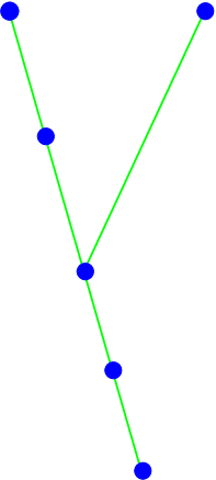
We have then:

\min\{P,\langle L,P,A\rangle\}=P,\quad\min\{Q,\langle L,Q,A\rangle\}=T.

As the function ${\mathbf{c}}_{L}$ is strictly increasing on $\Theta_{L}(C)$ and $P\prec_{L}T$ , we deduce that ${\mathbf{c}}_{L}(P)<{\mathbf{c}}_{L}(T)$ . By Proposition 8.17, we conclude that $V_{L}^{P}(A)<V_{L}^{Q}(A)$ .

– Assume that $P$ and $Q$ are incomparable for $\preceq_{L}$ .

Denote $I:=P\wedge_{L}Q=\langle L,P,Q\rangle$ . We have the strict inequalities $I\prec_{L}P$ , $I\prec_{L}Q$ . Choose a rational point $T\in(I,Q)$ . Therefore there exists a branch $A$ on $S$ such that its attaching point in $\Theta_{L}(C)$ is the point $T$ (see Figure 16).

We deduce that:

\min\{P,\langle L,P,A\rangle\}=\min\{P,I\}=I,\mbox{ and }\min\{Q,\langle L,Q,A\rangle\}=\min\{Q,T\}=T.

As the function ${\mathbf{c}}_{L}$ is strictly increasing on $\Theta_{L}(C)$ and $I\prec_{L}T$ , we deduce that ${\mathbf{c}}_{L}(I)<{\mathbf{c}}_{L}(T)$ . By Proposition 8.17, we conclude that $V_{L}^{P}(A)<V_{L}^{Q}(A)$ .

$\bullet$ The map $V_{L}$ is continuous. It is enough to prove that $V_{L}$ is continuous when $C$ is a branch. By the definition of the weak topology on the semivaluation space $\mathcal{V}$ , this amounts to proving the continuity of the following map:

\left\{\begin{array}[]{ccc}\Theta_{L}(C)&\to&[0,\infty]\\ P&\to&V_{L}^{P}(A)\end{array}\right.

for any fixed branch $A$ . But this is an immediate consequence of Proposition 8.17.

$\bullet$ The map $V_{L}$ sends $L$ to $\mbox{ord}^{L}$ and $C_{i}$ to $I_{L}^{C_{i}}$ . This follows from Remark 8.14.

$\bullet$ The map $V_{L}$ identifies ${\mathbf{c}}_{L}$ with ${\mathbf{s}}_{L}$ . We will prove this in restriction to the rational points of $\Theta_{L}(C)$ . Such a point is the center $\langle L,C_{i},A\rangle$ of a tripod, where $C_{i}$ is a branch of $C$ and $A$ is a certain branch on $S$ . We may assume as before that $C$ is irreducible (therefore $C_{i}=C$ ), and that we look at the point $\langle L,C,A\rangle$ . Then the fact that $V_{L}$ is continuous, injective and increasing implies that $V_{L}^{\langle L,C,A\rangle}=\langle\mbox{ord}^{L},I^{C}_{L},I^{A}_{L}\rangle$ .

By Theorem 3.25, we have:

{\mathbf{c}}_{L}(\langle L,C,A\rangle)=\frac{(C\cdot A)}{(L\cdot C)(L\cdot A)}.

By Theorem 7.20, we also have:

{\mathbf{s}}_{L}(\langle\mbox{ord}^{L},I^{C}_{L},I^{A}_{L})\rangle)=\frac{{\langle I^{C},I^{A}\rangle}}{{\langle\mbox{ord}^{L},I^{C}\rangle}{\langle\mbox{ord}^{L},I^{A}\rangle}}.

Proposition 7.8 shows then that the right-hand sides of the two previous equalities coincide.

As the statement is true for the rational points, which are dense in $\Theta_{L}(C)$ , and both ${\mathbf{c}}_{L}$ and ${\mathbf{s}}_{L}$ are continuous, we deduce that the statement is true for all points.

$\bullet$ The map $V_{L}$ identifies ${\mathbf{i}}_{L}$ with ${\mathbf{m}}_{L}$ . We reason analogously, by first proving the statement for rational points of $\Theta_{L}(C)$ . Let $P$ be such a point. We may choose a branch $A$ such that $P\in\Theta_{L}(A)$ and ${\mathbf{i}}_{L}(P)={\mathbf{i}}_{L}(A)={\langle I^{L},A\rangle}$ . Moreover, in this case ${\langle I^{L},A\rangle}=\min\{{\langle I^{L},A^{\prime}\rangle}\ |\ P\preceq_{L}A^{\prime}\}.$ By definition, this last minimum is ${\mathbf{m}}_{L}(V_{L}^{P})$ . The conclusion follows.

$\bullet$ The map $V_{L}$ identifies $1+{\mathbf{e}}_{L}$ with ${\mathbf{l}}_{L}$ . As a direct consequence of the differential relations $d{\mathbf{l}}_{L}={\mathbf{m}}_{L}\>d{\mathbf{s}}_{L}$ and $d{\mathbf{e}}_{L}={\mathbf{i}}_{L}\>d{\mathbf{c}}_{L}$ , we see that there exists a constant $a\in{\mathbb{R}}$ such that ${\mathbf{e}}_{L}+a$ is sent to ${\mathbf{l}}_{L}$ by the map $V_{L}$ . As ${\mathbf{e}}_{L}(L)=0$ and ${\mathbf{l}}_{L}(\mathrm{ord}^{L})=1$ , we deduce that $a=1$ . ∎

Remark 8.20.

As it was the case with the Eggers-Wall tree $\Theta_{L}(C)$ itself, the map $V_{L}$ depends only on $C$ and on the smooth branch $L$ defined by $x$ . Namely, $V_{L}^{P}$ is the unique semivaluation of the segment $[\mathrm{ord}^{L},I^{C}_{L}]\subset\mathcal{V}_{L}$ whose self-interaction is equal to ${\mathbf{c}}_{L}(P)$ .

Remark 8.21.

A variant of the map $V_{L}$ was already defined by Favre and Jonsson in [8, Prop. D1, page 223]. They started from a generic Eggers-Wall tree and a generic version of the exponent function. They associated to any point of it of exponent $e$ , situated on the segment $[O,C_{i}]$ , the unique point of the segment $[I^{O},I^{C_{i}}_{O}]$ with log-discrepancy $1+e$ relative to $O$ . They did not give another interpretation of that map, for instance analogous to our definition (8.2).

The following lemma proves that if $\nu$ and $\nu^{\prime}$ are two different semivaluations in $\mathcal{V}_{L}$ , then there exists a branch $A$ such that the attaching points of $\nu$ and $\nu^{\prime}$ on the segment $[\mathrm{ord}^{L},I^{A}_{L}]$ are different.

Lemma 8.22.

(1)

Let $\nu$ and $\nu^{\prime}$ be two different semivaluations in $\mathcal{V}_{L}$ . Then, there exists a branch $A$ such that $\nu(A)\neq\nu^{\prime}(A)$ .
(2)

If $A$ is such a branch, denote by $P=\langle\mathrm{ord}^{L},I^{A}_{L},\nu\rangle$ the center of the tripod determined by the normalized semivaluations $\mathrm{ord}^{L},I^{A}_{L}$ and $\nu$ on the tree $\mathcal{V}_{L}$ , and denote similarly $P^{\prime}=\langle\mathrm{ord}^{L},I^{A}_{L},\nu^{\prime}\rangle$ . Then, we have that $P\neq P^{\prime}$ .

Proof.

Assume that $\nu(A)=\nu^{\prime}(A)$ for any branch $A$ . Then, if $h\in\mathcal{O}$ , we have that $h=\prod_{j}h_{j}$ with $h_{j}$ irreducible. By hypothesis the semivaluations $\nu$ and $\nu^{\prime}$ have the same value on the branch $A_{j}=Z(h_{j})$ . It follows that $\nu(h)=\sum_{j}\nu(A_{j})=\nu^{\prime}(h)$ . This proves the first statement.

By the tripod formula (7.22) we get the relations:

(8.23)

{\mathbf{s}}_{L}(P)=\frac{{\langle\nu,I^{A}\rangle}}{{\langle I^{L},\nu\rangle}\>{\langle I^{L},I^{A}\rangle}}\mbox{ and }{\mathbf{s}}_{L}(P^{\prime})=\frac{{\langle\nu^{\prime},I^{A}\rangle}}{{\langle I^{L},\nu\rangle}\>{\langle I^{L},I^{A}\rangle}}.

By Proposition 7.8, we have that:

\begin{array}[]{lclclcl}{\langle\nu,I^{L}\rangle}&=&\nu(L),&&{\langle\nu^{\prime},I^{L}\rangle}&=&\nu^{\prime}(L),\\ {\langle\nu,I^{A}\rangle}&=&\nu(A),&&{\langle\nu^{\prime},I^{A}\rangle}&=&\nu^{\prime}(A),\end{array}

and ${\langle I^{L},I^{A}\rangle}=(L\cdot A)$ . In addition, $\nu(L)=\nu^{\prime}(L)=1$ since $\nu$ and $\nu^{\prime}$ belong to $\mathcal{V}_{L}$ . It follows that $L\neq A$ hence $(L\cdot A)\in{\mathbb{N}}^{*}$ . Since $\nu(A)\neq\nu^{\prime}(A)$ it follows from (8.23) that ${\mathbf{s}}_{L}(P)\neq{\mathbf{s}}_{L}(P^{\prime})$ . Since the restriction to ${\mathbf{s}}_{L}$ to the segment $[\mathrm{ord}^{L},I^{A}_{L}]$ is strictly increasing and $P,P^{\prime}$ belongs to this segment it follows that $P\neq P^{\prime}$ , which proves the second statement. ∎

We prove now that the semivaluation space $\mathcal{V}_{L}$ is the projective limit of the Eggers-Wall trees $\Theta_{L}(C)$ of reduced plane curves, embedded by the map $V_{L}$ .

Theorem 8.24.

Let us denote by $\mathcal{B}$ the set of branches at $O$ on the smooth surface $S$ and by $J$ the set consisting of finite subsets of $\mathcal{B}$ . For any $j\in J$ , we denote by $C_{j}$ the reduced plane curve singularity whose branches are the elements of the set $j$ . Denote by $\mathcal{V}_{L,j}$ the subtree $\mathcal{V}_{L}(\Theta_{L}(C_{j}))$ of $\mathcal{V}_{L}$ . The collection $(\mathcal{V}_{L,j})_{j\in J}$ forms a projective system for the inclusion partial order. If $\mathcal{V}_{L,j}\subset\mathcal{V}_{L,l}$ , we denote by $\pi^{l}_{L,j}:\mathcal{V}_{L,l}\to\mathcal{V}_{L,j}$ the corresponding attaching map. Then:

(1)

The maps $\pi_{L,j}^{l}$ form a projective system of continuous maps.
(2)

The attaching maps $\pi_{L,j}:\mathcal{V}_{L}\to\mathcal{V}_{L,j}$ glue into a homeomorphism $\pi_{L}:\mathcal{V}_{L}\to\displaystyle{\lim_{\longleftarrow}}\>\mathcal{V}_{L,j}$ .

Proof.

The collection $(\mathcal{V}_{L,j})_{j\in J}$ form a projective system for the inclusion partial order, since for any $j,k\in J$ there exists $l=j\cup k\in J$ such that $\mathcal{V}_{L,j}\subset\mathcal{V}_{L,l}$ and $\mathcal{V}_{L,k}\subset\mathcal{V}_{L,l}$ .

Notice that if $\mathcal{V}_{L,j}\subset\mathcal{V}_{L,l}$ , we can understand the attaching map $\pi^{l}_{L,j}:\mathcal{V}_{L,l}\to\mathcal{V}_{L,j}$ by using the embedding $V_{L}$ , since for any $P\in\Theta_{L}(C_{l})$ we have

\pi^{l}_{L,j}(V_{L}(P))=V_{L}(\pi_{\Theta_{L}(C_{j})}(P)),

where $\pi_{\Theta_{L}(C_{j})}:\Theta_{L}(C_{l})\to\Theta_{L}(C_{j})$ , is the surjective attaching map of Definition 2.11 (whose image is $\Theta_{L}(C_{j})\subset\Theta_{L}(C_{l})$ ). This implies that the maps $\pi_{L,j}^{l}$ form a projective system of continuous maps.

Now we apply Theorem 2.14 in this setting:

– The only hypothesis we need to check is point (4) in Theorem 2.14. This hypothesis hold by Lemma 8.22.

– Recall that the semivaluation space $\mathcal{V}_{L}$ is compact. Therefore, Theorem 2.14, applied to the projective system $\pi_{L,j}^{l}$ , implies that the map $\pi_{L}:\mathcal{V}_{L}\to\displaystyle{\lim_{\longleftarrow}}\>\mathcal{V}_{L,j}$ is a homeomorphism. ∎

In order to be able to compare the points of Eggers-Wall trees of various curves relative to various smooth branches considered as their roots, we embed them also in the fixed projective semivaluation tree $\mathbb{P}(\mathcal{V})$ , instead of doing it in the varying trees $\mathcal{V}_{L}$ :

Definition 8.25.

The valuative embedding of the Eggers-Wall tree $\Theta_{L}(C)$ is the map $\Psi_{L}:=\pi_{L}\circ V_{L}:\Theta_{L}(C)\to\mathbb{P}(\mathcal{V})$ .

9. Change of observer on the semivaluation space

It is important to know how to change coordinates when one changes the observer. The aim of this section is to prove formulae expressing the functions $({\mathbf{l}}_{R^{\prime}},\mathbf{m}_{R^{\prime}},{\mathbf{s}}_{R^{\prime}})$ in terms of the functions $({\mathbf{l}}_{R},\mathbf{m}_{R},{\mathbf{s}}_{R})$ , whenever $R$ and $R^{\prime}$ are two distinct observers of the valuative tree ${\mathbb{P}}(\mathcal{V})$ . Combined with the embedding theorem 8.19, these formulae of changes of coordinates are the main ingredients of the proof of the generalized inversion theorem 4.5.

The following proposition is an immediate consequence of Definition 7.9:

Proposition 9.1.

Let $R,R^{\prime}$ be two observers of $\mathbb{P}(\mathcal{V})$ . Then one has the following formulae of change of coordinates from $R$ to $R^{\prime}$ :

(9.2)

{\mathbf{l}}_{R^{\prime}}=\gamma^{R}_{R^{\prime}}\cdot{\mathbf{l}}_{R},

(9.3)

{\mathbf{s}}_{R^{\prime}}=(\gamma^{R}_{R^{\prime}})^{2}\cdot{\mathbf{s}}_{R},

where:

(9.4)

\gamma^{R}_{R^{\prime}}(P)=\frac{{\langle\nu^{P},I^{R}\rangle}}{{\langle\nu^{P},I^{R^{\prime}}\rangle}}

for any projective semivaluation $P\in\mathbb{P}(\mathcal{V})$ . Here $\nu^{P}\in\mathcal{V}$ is an arbitrary semivaluation representing $P$ .

Remark 9.5.

Seen as functions on $\mathbb{P}(\mathcal{V})$ , one has $\gamma^{R}_{R^{\prime}}\cdot\gamma_{R}^{R^{\prime}}=1$ .

The function $\gamma^{R}_{R^{\prime}}$ is expressed in the following way in terms of the relative interaction and self-interaction functions:

Proposition 9.6.

Assume that $R,R^{\prime}$ are distinct observers on $\mathbb{P}(\mathcal{V})$ . Then:

\gamma^{R}_{R^{\prime}}(P)=({\langle I^{R},I^{R^{\prime}}\rangle}\cdot{\mathbf{s}}_{R}(\langle R,R^{\prime},P\rangle))^{-1}\mbox{ for any }P\in\mathbb{P}(\mathcal{V}).

In particular, if $R$ and $R^{\prime}$ are transversal smooth branches, we have:

\gamma^{R}_{R^{\prime}}(P)={\mathbf{s}}_{R}(\langle R,R^{\prime},P\rangle)^{-1}=({\mathbf{l}}_{R}(\langle R,R^{\prime},P\rangle)-1)^{-1}\mbox{ for any }P\in\mathbb{P}(\mathcal{V}).

Proof.

The first equality is an immediate consequence of the tripod formula (7.22). The last equality is a consequence of formula (7.17) and of the fact that ${\mathbf{m}}_{R}$ is identically equal to $1$ on the segment $[L,L^{\prime}]\subset\mathbb{P}(\mathcal{V})$ , when $R$ and $R^{\prime}$ are transversal smooth branches. This last fact is a consequence of the Definition 7.10 of the relative multiplicity function. ∎

There is also a formula of change of coordinates for the relative multiplicity functions:

Proposition 9.7.

Let $R,R^{\prime}$ be two distinct observers on $\mathbb{P}(\mathcal{V})$ . Then (see Figure 17):

(9.8)

{\mathbf{m}}_{R^{\prime}}=\left\{\begin{array}[]{ll}1&\mbox{ on }[R^{\prime},\ \langle R,R^{\prime},O\rangle],\\ {\langle I^{R},I^{R^{\prime}}\rangle}&\mbox{ on }(\langle R,R^{\prime},O\rangle,\ R],\\ \gamma_{R}^{R^{\prime}}\cdot{\mathbf{m}}_{R}&\mbox{ on }\mathbb{P}(\mathcal{V})\>\setminus\>[R^{\prime},R].\end{array}\right.

Proof.

We prove the formulae when both observers are smooth branches $R=L,R^{\prime}=L^{\prime}$ , leaving to the reader the analogous reasoning in the remaining case when one of the observers is the point $O$ . We will consider successively the three possibilities listed in the previous formula for the position of the point $P\in\mathbb{P}(\mathcal{V})$ relative to the tripod determined by $O,L,L^{\prime}$ .

$\bullet$ Assume that $P\in[L^{\prime},\ \langle L,L^{\prime},O\rangle]$ . Consider a third smooth branch $M$ , transversal to $L^{\prime}$ (see Figure 18). Then $O\in[L^{\prime},M]$ and ${\mathbf{m}}_{L^{\prime}}$ is constantly equal to $1$ on $[L^{\prime},M]$ . As $[L^{\prime},\ \langle L,L^{\prime},O\rangle]\subset[L^{\prime},O]$ , we deduce the desired relation ${\mathbf{m}}_{L^{\prime}}(P)=1$ .

$\bullet$ Assume that $P\in(\langle L,L^{\prime},O\rangle,\ L]$ . Apply then formula (7.15) to ${\mathbf{m}}_{L^{\prime}}(P)$ :

(9.9)

{\mathbf{m}}_{L^{\prime}}(P)=\lim_{P_{-}\to P,\,\,P_{-}\prec_{L^{\prime}}P}\,\,\,\dfrac{{\mathbf{l}}_{L^{\prime}}(P)-{\mathbf{l}}_{L^{\prime}}(P_{-})}{{\mathbf{s}}_{L^{\prime}}(P)-{\mathbf{s}}_{L^{\prime}}(P_{-})}.

In order to compute the limit (9.9) we can assume that $P_{-}\in(\langle L,L^{\prime},O\rangle,\ L]$ . Take then an auxiliary point $Q\in(\langle L,L^{\prime},O\rangle,\ L]$ (see Figure 19). Our choice implies that $\langle O,L^{\prime},Q\rangle=\langle L,L^{\prime},O\rangle$ .

By Proposition 9.6 and the tripod formula (7.22) we deduce that:

(9.10)

\gamma^{O}_{L^{\prime}}(Q)=({\langle I^{O},I^{L^{\prime}}\rangle}\cdot{\mathbf{s}}_{O}(\langle O,L^{\prime},Q\rangle))^{-1}={\mathbf{s}}_{O}(\langle L,L^{\prime},O\rangle)^{-1}=(L\cdot L^{\prime})^{-1}.

We pass now from the observer $L^{\prime}$ to $O$ . That is, we apply the formulae (9.2) and (9.3) to (9.9), with $R^{\prime}=L^{\prime}$ and $R=O$ .

By (9.10) the value of $\gamma^{O}_{L^{\prime}}$ is constant on the segment $(\langle L,L^{\prime},O\rangle,\ L]$ and we may factor it when computing the limit in (9.9). We get:

(9.11)

{\mathbf{m}}_{L^{\prime}}(P)=(L\cdot L^{\prime})\,\,\lim_{P_{-}\to P,\,\,P_{-}\prec_{L^{\prime}}P}\,\,\,\,\dfrac{{\mathbf{l}}_{O}(P)-{\mathbf{l}}_{O}(P_{-})}{{\mathbf{s}}_{O}(P)-{\mathbf{s}}_{O}(P_{-})}.

Since $P_{-}\in(\langle L,L^{\prime},O\rangle,\ L]$ , we have that $P_{-}\prec_{L^{\prime}}P$ is equivalent to $P_{-}\prec_{O}P$ . Therefore, the limit (9.11) is equal to $\mathbf{m}_{O}(P)$ . Notice that $m_{O}$ is constantly equal to $1$ on $[O,L]\supset(\langle L,L^{\prime},O\rangle,P)$ , thus $\mathbf{m}_{O}(P)=1$ . By Proposition 7.8, we get the desired equality ${\mathbf{m}}_{L^{\prime}}(P)=(L\cdot L^{\prime})={\langle I^{L},I^{L^{\prime}}\rangle}$ .

$\bullet$ Assume that $P\in\mathbb{P}(\mathcal{V})\>\setminus\>[L,L^{\prime}]$ . Here the reasoning is analogous to the one done in the previous case, but instead of changing coordinates by replacing the observer $L^{\prime}$ with $O$ , one replaces it with $L$ . The main point is that one may compute the limit (9.9) by restricting the points $P_{-}$ to the segment $(\langle L,L^{\prime},P\rangle,\ P)$ . This implies that $\langle L,L^{\prime},P_{-}\rangle=\langle L,L^{\prime},P\rangle$ (see Figure 20).

In particular, by Proposition 9.6, we get that $\gamma^{L}_{L^{\prime}}(P_{-})=\gamma^{L}_{L^{\prime}}(P)$ . Therefore one may factor $\gamma^{L}_{L^{\prime}}(P)$ in the numerator and $(\gamma^{L}_{L^{\prime}}(P))^{2}$ in the denominator of the fraction in formula (9.9), which implies by Remark 9.5 that:

{\mathbf{m}}_{L^{\prime}}(P)=\gamma_{L}^{L^{\prime}}(P)\cdot\,\,\lim_{P_{-}\to P,\,P_{-}\prec_{L^{\prime}}P}\,\,\,\,\dfrac{{\mathbf{l}}_{L}(P)-{\mathbf{l}}_{L}(P_{-})}{{\mathbf{s}}_{L}(P)-{\mathbf{s}}_{L}(P_{-})}.

But one has also the inequality $P_{-}\prec_{L}P$ , as $P_{-}\in(\langle L,L^{\prime},P\rangle,P)$ . By (7.15), this implies that the last limit is equal to ${\mathbf{m}}_{L}(P)$ . We get the desired relation ${\mathbf{m}}_{L^{\prime}}(P)=\gamma_{L}^{L^{\prime}}(P)\cdot{\mathbf{m}}_{L}(P)$ . ∎

References

[1] Abhyankar, S. S. Inversion and invariance of characteristic pairs. American Journal of Maths. 89 (1967), 363–372.
[2] Baker, M., Rumely, R. Potential theory and dynamics on the Berkovich projective line. Math. Surveys and Monographs 159, AMS, 2010.
[3] Barth, W.P., Hulek, K., Peters, C.A.M., Van de Ven, A. Compact complex surfaces. Second edition. Ergebnisse der Mathematik und ihrer Grenzgebiete. 3. Folge. A Series of Modern Surveys in Mathematics 4. Springer-Verlag, Berlin, 2004.
[4] Berkovich, V.G. Spectral theory and analytic geometry over non-Archimedean fields. Math. Surveys and Monographs 33, AMS, 1990.
[5] Corral, N. Sur la topologie des courbes polaires de certains feuilletages singuliers. Ann. Inst. Fourier (Grenoble), 53, (2003), no. 3, 787–814.
[6] Eggers, H. Polarinvarianten und die Topologie von Kurvensingularitaeten. Bonner Math. Schriften 147, 1983.
[7] Eisenbud, D., Neumann, W. Three-dimensional link theory and invariants of plane curve singularities. Princeton Univ. Press, 1985.
[8] Favre, C., Jonsson, M. The valuative tree. Lect. Notes in Maths. 1853. Springer-Verlag, Berlin, 2004.
[9] García Barroso, E. R. Invariants des singularités de courbes planes et courbure des fibres de Milnor. PhD thesis, Univ. La Laguna, Tenerife (Spain), 1996. Available at http://ergarcia.webs.ull.es/tesis.pdf.
[10] García Barroso, E. R., Sur les courbes polaires d’une courbe plane réduite, Proc. London Math. Soc. (3) 81 (2000) 1–28.
[11] García Barroso, E. R., González Pérez, P. D. Decomposition in bunches of the critical locus of a quasi-ordinary map. Compositio Math. 141 (2005), 461–486.
[12] García Barroso, E. R., González Pérez, P. D., Popescu-Pampu, P., Variations on inversion theorems for Newton-Puiseux series, Math. Ann. 368, (2017), no. 3-4, 1359–1397.
[13] García Barroso, E. R., González Pérez, P. D., Popescu-Pampu, P. Ultrametric spaces of branches on arborescent singularities. To appear in Singularities, Algebraic Geometry, Commutative Algebra and Related Topics. Festschrift for Antonio Campillo on the Occasion of his 65th Birthday. G.-M. Greuel, L. Narváez and S. Xambó-Descamps eds. Springer, 2018. 52 pages.
[14] García Barroso, E. R., González Pérez, P. D., Popescu-Pampu, P., M. Ruggiero, Ultrametric properties for valuation spaces of normal surface singularities. preprint 2018, ArXiv:1802.01165.
[15] Guibert, G., Loeser, F., Merle, M. Composition with a two variable function. Math. Research Letters 16 No. 3 (2009), 439–448.
[16] Halphen, G. Sur une série de courbes analogues aux développées. Journal de maths. pures et appliquées (de Liouville) 3e série, tome 2 (1876), 87–144.
[17] Hocking, J. G., Young, G. S., Topology. Constable and Company, Ltd., 1961, reprinted by Dover Publications, 1988.
[18] Jonsson, M. Dynamics on Berkovich spaces in low dimensions. In Berkovich spaces and applications, 205–366. A. Ducros, C. Favre, J. Nicaise eds., Lect. Notes in Maths. 2119, 2015.
[19] Kapranov, M. M. Veronese curves and Grothendieck-Knudsen moduli space $\overline{M}_{0,n}$ . J. Algebraic Geom. 2 (1993), no. 2, 239–262.
[20] Kapranov, M. M. The permutoassociahedron, Mac Lane’s coherence theorem and asymptotic zones for the KZ equation. J. Pure Appl. Algebra 85 (1993), no. 2, 119–142.
[21] Kuo, T.C., Lu, Y.C. On analytic function germs of two complex variables. Topology 16 (1977), no. 4, 299–310.
[22] McNeal J.D., Némethi, A. The order of contact of a holomorphic ideal in ${\mathbb{C}}^{2}$ . Math. Zeitschrift, 250 (4) (2005), 873–883.
[23] Noether, M. Les combinaisons caractéristiques dans la transformation d’un point singulier. Rend. Circ. Mat. Palermo IV (1890), 89-108, 300–301.
[24] Novacoski, J. Valuations centered at a two-dimensional regular local ring: infima and topologies., Valuation theory in interaction, EMS Ser. Congr. Rep., 389–403, 2014.
[25] Orlik, P. Seifert manifolds. Lecture Notes in Mathematics 291. Springer-Verlag, Berlin-New York, 1972.
[26] Płoski, A. Remarque sur la multiplicité d’intersection des branches planes. Bulletin of the Polish Academy of Sciences. Mathematics. Volume 33 (1985), 601–605.
[27] Popescu-Pampu, P. Arbres de contact des singularités quasi-ordinaires et graphes d’adjacence pour les 3-variétés réelles. Thèse, Univ. Paris 7, 2001. Available at https://tel.archives-ouvertes.fr/tel-00002800v1.
[28] Popescu-Pampu, P. Sur le contact d’une hypersurface quasi-ordinaire avec ses hypersurfaces polaires. Journal of the Inst. of Math. Jussieu 3 (2004), 105–138.
[29] Shafarevich, I. Basic algebraic geometry. Vol. 1,2. Springer-Verlag, 1994.
[30] Siebenmann, L. On vanishing of the Rohlin invariant and non-finitely amphicheiral homology $3$ -spheres. In Topology Symposium, Siegen, 1979, Koschorke and Neumann eds., Lecture Notes in Maths. 788 (1979), 172–222.
[31] Smith, H.J.S. On the higher singularities of plane curves. Proc. London Math. Soc., Vol. VI (1875), 153–182.
[32] Stolz, O. Die Multiplicität der Schnittpunkte zweier algebraischer Curven. Math. Annalen 15 (1879), 122–160.
[33] Wall, C. T. C. Chains on the Eggers tree and polar curves. Proc. of the Int. Conf. on Algebraic Geometry and Singularities (Sevilla, 2001). Rev. Mat. Iberoamericana 19 (2003), no. 2, 745–754.
[34] Wall, C. T. C. Singular points of plane curves. London Math. Society Student Texts 63. Cambridge Univ. Press, 2004.
[35] Zariski, O. Studies in equisingularity III. Saturation of local rings and equisingularity. Amer. J. Math. 90 (1968), 961–1023.

The valuative tree is the projective limit of Eggers-Wall trees

Abstract.

Key words and phrases:

2010 Mathematics Subject Classification

1. Introduction

2. Finite trees and ℝ{\mathbb{R}}-trees

Definition 2.1.

Definition 2.2.

Definition 2.3.

Definition 2.4.

Definition 2.5.

Remark 2.6.

Definition 2.7.

Remark 2.8.

Example 2.9.

Lemma 2.10.

Definition 2.11.

Lemma 2.12.

Proof.

Definition 2.13.

Theorem 2.14.

3. Curve singularities and their Eggers-Wall trees

Definition 3.1.

Example 3.2.

Example 3.3.

Definition 3.4.

Definition 3.5.

Definition 3.6.

Definition 3.7.

Definition 3.8.

Proposition 3.9.

Lemma 3.10.

Remark 3.11.

Example 3.12.

Remark 3.13.

Remark 3.14.

Definition 3.15.

Remark 3.16.

Remark 3.18.

Remark 3.21.

Corollary 3.22.

Lemma 3.23.

Definition 3.24.

Theorem 3.25.

Remark 3.27.

Corollary 3.28.

Example 3.29.

4. An inversion theorem for Eggers-Wall trees

Definition 4.1.

Lemma 4.2.

Proof.

Example 4.3.

Definition 4.4.

Theorem 4.5.

Proof.

Corollary 4.7.

Remark 4.8.

Remark 4.9.

Example 4.10.

Remark 4.11.

5. Eggers-Wall trees and splice diagrams

Definition 5.1.

Definition 5.2.

Definition 5.3.

Proposition 5.4.

Lemma 5.5.

Definition 5.6.

Definition 5.7.

Definition 5.8.

Proposition 5.9.

Remark 5.10.

Definition 5.11.

Proposition 5.12.

Theorem 5.13.

Theorem 5.14.

Proof.

Remark 5.15.

Example 5.16.

6. Semivaluation spaces

Definition 6.1.

The valuative tree
is the projective limit of Eggers-Wall trees

2. Finite trees and ${\mathbb{R}}$ -trees