White Dwarf Pollution by Asteroids from Secular Resonances
Abstract
In the past few decades, observations have revealed signatures of metals polluting the atmospheres of white dwarfs. The diffusion timescale for metals to sink from the atmosphere of a white dwarf is of the order of days for a hydrogen-dominated atmosphere. Thus, there must be a continuous supply of metal-rich material accreting onto these white dwarfs. We investigate the role of secular resonances that excite the eccentricity of asteroids allowing them to reach star-grazing orbits leading them to tidal disruption and the formation of a debris disc. Changes in the planetary system during the evolution of the star lead to a change in the location of secular resonances. In our Solar System, the engulfment of the Earth will cause the resonance to shift outwards which will force previously stable asteroids to undergo secular resonant perturbations. With analytic models and –body simulations we show that secular resonances driven by two outer companions can provide a source of continuous pollution. Secular resonances are a viable mechanism for the pollution of white dwarfs in a variety of exoplanetary system architectures.
Keywords:
minor planets, asteroids: general – planets and satellites: dynamical evolution and stability – stars: AGB and post-AGB – (stars:) white dwarfs1 Introduction
About to of all white dwarfs have metal-polluted atmospheres identified by metallic absorption lines from spectroscopic measurements and a total of about white dwarfs are known to be polluted (Cottrell & Greenstein, 1980; Koester et al., 1982; Lacombe et al., 1983; Zeidler-K.T. et al., 1986; Koester et al., 1997; Zuckerman et al., 2003; Klein et al., 2010; Vennes et al., 2010; Zuckerman et al., 2010; Farihi et al., 2012; Farihi et al., 2014; Melis & Dufour, 2017, e.g.). These findings appear at first glance to be puzzling since white dwarf atmospheres stratify chemical elements through gravitational settling (Koester & Wilken, 2006; Koester, 2009). Once the white dwarf has cooled below , metals are no longer supported by radiative forces and rapidly sink and diffuse within the white dwarf’s atmosphere due to the intense gravity environment (Fontaine & Michaud, 1979; Vauclair et al., 1979; Koester, 2009). It is noteworthy that white dwarfs are observed in a temperature range from K to K (Fontaine et al., 2001), which coincides with cooling ages of to , respectively (Koester et al., 2014). The stratification or diffusion timescales for metals are of the order of days to weeks for DA (hydrogen atmosphere) white dwarfs and yrs for DB (helium atmosphere) white dwarfs (Koester & Wilken, 2006). This implies that the diffusion timescale of metals is many orders of magnitude shorter than the white dwarf cooling time (Paquette et al., 1986). Accretion discs and pollution are observed at to cooling ages (Farihi, 2016). Thus, these polluted white dwarfs need to be continuously accreting metal-rich material in order for the metal absorption lines to be observable.
Several theoretical models have been explored to explain the metal pollution. Accretion of metallic material originating from the interstellar medium has been conclusively ruled out by Farihi et al. (2010a) (Aannestad et al., 1993; Jura, 2006; Kilic & Redfield, 2007; Barstow et al., 2014, see also). The currently favored pollution mechanism suggests that metal-rich planetary material is tidally disrupted (due to close encounters with the star) into a debris disc and then subsequently accreted onto the white dwarf (Gänsicke et al., 2006; Kilic et al., 2006; von Hippel et al., 2007; Farihi et al., 2009; Jura et al., 2009; Farihi et al., 2010b; Melis et al., 2010; Brown et al., 2017; Bonsor et al., 2017; Xu et al., 2018). For a recent review on the dynamics of white dwarf pollution, see Farihi (2016). The sources of pollution that have been proposed include asteroids (Jura, 2003; Jura, 2006; Jura et al., 2009; Debes et al., 2012; Veras et al., 2013; Wyatt et al., 2014), comets (Caiazzo & Heyl, 2017), moons via planet-planet scattering (Payne et al., 2016; Payne et al., 2017) and perturbations of planetary material due to eccentric planets (Frewen & Hansen, 2014). Perturbations may also be caused by Kozai-Lidov instabilities in stellar binaries (Hamers & Portegies Zwart, 2016; Petrovich & Muñoz, 2017). Veras et al. (2017) recently formulated the critical separation of binaries in order for the stellar companion to produce pollution of white dwarf atmospheres by Roche lobe overflow or by stellar winds. Their findings suggested that the critical separation is only a few astronomical units (au), which means that this mechanism is inefficient for wide binary systems.
The chain of events is thought to be as follows. As a main-sequence star evolves, the star undergoes significant mass loss during the red-giant branch (RGB) phase (Reimers, 1977; McDonald & Zijlstra, 2015) and during the asymptotic giant branch (AGB) phase (Rosenfield et al., 2014; Rosenfield et al., 2016). This mass loss is a result of radiation pressure pushing on the loosely bound outer layers of the red giant. The mass outflow, or stellar wind, leads to mass-loss rates of up to (Veras et al., 2011, e.g.) that depletes the star of a large fraction of its initial mass. During the expansion of the outer envelop, close-in planets are engulfed (Siess & Livio, 1999; Villaver & Livio, 2007; Villaver & Livio, 2009; Mustill & Villaver, 2012; Adams & Bloch, 2013; Villaver et al., 2014), leading (among other things) to dynamical changes within the system. As the star undergoes significant mass loss, due to conservation of angular momentum, the orbits of all surviving bodies expand outward (Duncan & Lissauer, 1998). For planets and asteroids that are at orbital radii well below a few hundred au of the star, the timescale for mass loss is much longer than the orbital periods of the planets and so the orbits of the planets and asteroids expand adiabatically (Veras et al., 2013).
To take our Solar system as an example, many asteroids are located in the asteroid belt between Mars and Jupiter. Over time, some asteroids undergo resonant gravitational perturbations from the two largest planets, Jupiter and Saturn, causing the asteroids to become scattered from the asteroid belt (Morbidelli et al., 1995; Gladman et al., 1997; Morbidelli & Gladman, 1998; Bottke et al., 2000; Petit et al., 2001; Ito & Malhotra, 2006; Brož & Vokrouhlický, 2008; Minton & Malhotra, 2010; Chrenko et al., 2015; Granvik et al., 2017). In a mean-motion resonance, the ratio of the orbital periods of two objects is an integer ratio (Armitage, 2013, e.g.). Secular resonances arise when the apsidal or nodal precession rates of two objects orbiting a central object are close (Froeschle & Scholl, 1986; Yoshikawa, 1987). Apsidal resonances are more important in the context of white dwarf pollution since apsidal resonances excite eccentricities, which can lead to tidal disruptions, whereas nodal resonances excite inclinations. The most important apsidal secular resonance in our solar system is the resonance (Bottke et al., 2000; Ito & Malhotra, 2006; Minton & Malhotra, 2011; Haghighipour & Winter, 2016; Smallwood et al., 2017, e.g.), that occurs between the apsidal precession of the asteroids and Saturn. The outer edge of the resonance sets the inner boundary to our asteroid belt at approximately . The region where Jupiter’s mean-motion resonances overlap is what determines the outer edge of the asteroid belt at about to . Each mean-motion resonance has a width, in semi-major axis, over which it operates (Dermott & Murray, 1983). The locations and widths of secular resonances are harder to constrain due to their strong dependences on the semi-major axis, eccentricity, and inclination (Knezevic et al., 1991). We use a first-order analytical approximation in section 2.1 to determine the locations and eccentricity excitation regions of these resonances. Asteroids close to the resonance location undergo perturbations causing their eccentricities to increase, eventually leading the asteroids to either be ejected from the solar system or collide with the central star. Regions in which the resonance widths overlap are known as chaotic regions (Murray & Holman, 1997; Murray & Holman, 1999), and there almost all of the asteroids are cleared out.
Debes et al. (2012) investigated white dwarf pollution by asteroids that originate from the 2:1 mean-motion resonance with Jupiter, which is presently located at (Nesvorný & Morbidelli, 1998; Petit et al., 2001). In their model, as the star loses mass through its stellar evolution, the libration width of the 2:1 resonance is slightly widened, forcing previously stable asteroids to eventually become accreted onto the white dwarf. We propose that secular resonances may provide an additional mechanism and source of pollution. If the planetary system undergoes major changes during the stellar evolution (for instance, if the inner planets are engulfed by the star), the secular frequencies of the whole planetary system are affected, resulting in a displacement of the location of secular resonances. On the other hand, the locations of mean-motion resonances with respect to the remaining planets remains almost unchanged. Ward (1981) discuses a similar process whereby secular resonances are affected by the mass loss of the solar nebula rather than the central star. The changes in the dynamics of these resonances may have aided in the accretion of planetesimals by growing terrestrial planets.
In the present work we investigate the evolution of an exoplanetary system that contains a white dwarf that harbors a planetary system and an asteroid belt. The giant outer planets and the asteroid belt are sufficiently far from the white dwarf so that they survive the stellar evolution through the RGB/AGB phases. We consider systems with two giant planets, like the solar system, and systems with one giant planet and a binary stellar companion. We explore how different system architectures are able to pollute the atmospheres of white dwarfs. In Section 2 we describe the analytical and numerical models that we use to calculate the location and dynamics of secular resonances that will occur within our Solar System as it evolves. In Section 3 we analyze white dwarf pollution for various architectures of exoplanetary systems. Finally, we draw our conclusions in Section 4.
2 Solar System
In this Section we first consider how our solar system will evolve once our Sun is on its way to becoming a white dwarf. We assume that the terrestrial planets, up to the orbital radius of the Earth, will become engulfed by the Sun (Rasio et al., 1996; Schröder & Connon Smith, 2008), while the orbits of the giant planets and the asteroid belt will expand adiabatically. We model the evolution of the resonance in the solar system first analytically and then numerically with –body simulations of the asteroid belt with the remaining planetary system. Even though Mercury and Venus will also be engulfed, we focus on the effects of the Earth engulfment. Because the Earth is more massive and located closer to the resonance it affects it more strongly.
2.1 Analytic Model
Here we examine the resonance location and the eccentricity excitation region for the resonance in the solar system both before and after the Sun becomes a white dwarf. The present-day values for the orbital elements are used for Earth, Jupiter, and Saturn. The secular resonance properties are mostly affected by both Saturn and Jupiter (Bottke et al., 2000; Ito & Malhotra, 2006). Jupiter increases the free precession frequency of the asteroids so that they fall into a resonance with an eigenfrequency that is dominated by Saturn. In this paper, the location of the resonance is estimated by calculating the location of the intersection of a test particle’s free precession rate with the eigenfrequency dominated by Saturn. The analytical model we use is linear in eccentricity and inclination and it gives the secular perturbations at first order to the orbital perturbation.
2.1.1 Eigenfrequencies
We consider a planetary system with a total of planets orbiting a central object with mass . Each planet has a semi–major axis , mass and orbital frequency , where . The eigenfrequencies are found by calculating the eigenvalues of the matrix associated with a generalized form of the secular perturbation theory
| (1) |
for and otherwise
| (2) |
(Murray & Dermott, 2000; Minton & Malhotra, 2011; Malhotra, 2012), where the Laplace coefficient is given by
| (3) |
and and are defined as
| (4) |
and
| (5) |
We find that the eigenfrequency has a value of (includes only Jupiter and Saturn) and a value of (includes all the planets in the Solar System), which is lower by roughly from the more accurate value of given by Brouwer & van Woerkom (1950) (see Laskar (1988) for further comparisons).
2.1.2 Asteroid free precession rates
We calculate the free precession rate of test particles in the potential of the planetary system. In this linear theory in eccentricity and inclination, it is only a function of the secular semi-major axis . The free precession rate is given by
| (6) |
(Murray & Dermott, 2000, e.g.), where is the orbital frequency of the test particle. The variables and are defined as
| (7) |
| (8) |
The mean precession frequency, , corresponds to the diagonal term of the Laplace-Lagrange matrix including the asteroid (Milani & Knezevic, 1990; Morbidelli & Henrard, 1991). In this work, we will first consider the case (Earth and Jupiter and Saturn), and after that take (Jupiter and Saturn) since the inner planets are engulfed during the RGB/AGB phases. The outer giants Neptune and Uranus do not significantly affect the dynamics of the asteroid belt (Izidoro et al., 2016, e.g.). Saturn also does not noticeably affect the free precession rate of the asteroids in the asteroid belt – that rate is dominated by Jupiter.
| Parameter | Symbol | Main-sequence value | Post-main-sequence value |
|---|---|---|---|
| Star Mass | |||
| Earth Mass | — | ||
| Jupiter Mass | |||
| Saturn Mass | |||
| Earth semi-major axis | — | ||
| Jupiter semi-major axis | |||
| Saturn semi-major axis | |||
| Earth Eccentricity | — | ||
| Jupiter Eccentricity | |||
| Saturn Eccentricity | |||
| Earth longitude of perihelion | — | ||
| Jupiter longitude of perihelion | |||
| Saturn longitude of perihelion | |||
| Location of resonance |
2.1.3 Resonance location
The semi-major axes of the planets are assumed to undergo adiabatic expansion based on the ratio of the initial stellar mass to the white dwarf mass,
| (9) |
Figure 1 shows the location of Jupiter, Saturn, and the secular resonance with the proper mode of Saturn as a function of white dwarf mass. We consider white dwarf masses in the range to as expected for the Sun (Liebert et al., 2005; Falcon et al., 2010; Tremblay et al., 2016). For our standard model we choose a mass of (Sackmann et al., 1993; Schröder & Connon Smith, 2008, e.g.). The location of the adiabatically expanded asteroid belt as a function of white dwarf mass is shown by the blue-shaded region. We use the observed inner and outer boundaries of the asteroid belt to produce this region, that is the range in semi-major axis. The observed inner boundary, created by the resonance, is consistent with our analytical model which places it at about .

2.1.4 Maximum Forced Eccentricity


In order to calculate the forced eccentricity excitation of a test particle near the secular resonance, we follow the procedure in Chapter 7 of Murray & Dermott (2000). We begin with the eccentricity part of the disturbing function, , from the secular theory for planets including a test particle with mean motion, , eccentricity, and longitude of the perihelion, , given by
| (10) |
where is the test particle free precession rate given in equation (6) and
| (11) |
The forced eccentricity is given by
| (12) |
where
| (13) |
and
| (14) |
The constants are determined from initial boundary conditions, is the dominant proper mode of the planet and is given by
| (15) |
where are the scaled eigenvector components corresponding to the eigenfrequencies found from equations (1) and (2), obtained from the initial conditions of the planetary system given in Table 1. The amplitudes of the orbital solution for the planets also depend on the longitudes of perihelion () of the planets. Thus we assume that all values are taken at present-day values. Since the time dependence in equations (13) and (14) are different during the main-sequence stage versus the post-main-sequence stage, we calculate the maximum forced eccentricity
| (16) |
Figure 2 shows the maximum forced eccentricity excitation of a test particle near the resonance during the main-sequence stage of stellar evolution (solid line) versus the post-main-sequence stage (dotted line). To obtain these curves we use the parameters presented in Table 1. The main sequence stage includes Earth, Jupiter and Saturn at semi-major axes , , and , respectively. The post-main-sequence stage only includes Jupiter and Saturn with semi-major axes of and , respectively, assuming that the Earth is engulfed during the RGB phase of stellar evolution. The -axis is normalized with respect to the semi-major axis of Jupiter in order to show the comparison. The resonance has shifted outwards into a region of the asteroid belt that would have previously contained stable asteroids. These asteroids are unstable to resonant perturbations and may be a source of pollution for white dwarfs. The amplitude of the shift is quite small compared to the crude approximation of the dynamics given by the linearized analytical model. The error within our analytical model is of some tenths of astronomical units in the location of the resonance, which is of the same order of magnitude of the shift. However, the mechanism we describe here is still qualitatively relevant. The shift could be much larger if a planet more massive than the Earth is engulfed. We investigate this further with numerical models in the next Section.
2.2 –body Simulations
We test the analytic models of the previous section with –body simulations of an asteroid belt around a white dwarf. We use the hybrid symplectic integrator in the orbital dynamics package, mercury, to model the structure of the asteroid belt and the tidal disruption rate around a white dwarf. mercury uses –body integrations to calculate the orbital evolution of objects moving in the gravitational field of a large body (Chambers, 1999). We simulated the motion of Jupiter, Saturn, and a distribution of asteroids orbiting a white dwarf star. The asteroids in our simulations are considered test particles which interact gravitationally with the planets and the white dwarf. We may neglect the asteroid-asteroid interactions because the timescale for such collisional interactions is much longer than the timescale for the action of perturbations by resonance effects. The timescale for resonant effects is of the order of (Ito & Tanikawa, 1999), whereas some of the largest asteroids have collisional timescales that are of the order of the age of the solar system (Dohnanyi, 1969). The general outcomes of test particles near secular and mean-motion resonances include ejections, collisions with a larger body, or remains within the simulation.
As the asteroids are scattered from the asteroid belt due to secular resonances, the asteroids become tidally disrupted by the white dwarf if they pass within a tidal disruption radius given by
| (17) |
(Davidsson, 1999; Jura, 2003; Bear & Soker, 2013), where , , are the mass, radius, and density of the white dwarf, respectively, and is the density of the asteroid. is a numerical constant that depends on the orbital parameters of the asteroid, its rotation, and composition (Davidsson, 1999; Jura, 2003). We take for a solid non-synchronized asteroid (Bear & Soker, 2013). We assume the average density of the asteroids to be (Krasinsky et al., 2002) in order to calculate the tidal disruption radius for the WD to be . Within our simulations, we artificially inflate the size of the white dwarf to have a radius equal to the tidal disruption radius. When an asteroid passes within the tidal disruption radius it is considered tidally disrupted and then removed from the simulation. The destabilization of asteroids should begin as soon as the Earth is engulfed, that is, when the Sun is still a red giant. Many objects will thus be ejected or will collide with the star before it reaches its white dwarf mass and radius. The evolution timescale between the red giant and white dwarf stages is around years. However, the timescale for resonant perturbations is on the order of years, thus in this work we assume that after the Earth engulfment, the Sun instantaneously shrinks to its white dwarf state in order to show the effects on the dynamics of secular resonances. We calculate the evolution of each asteroid orbit for a duration of million years, since this is longer than the cooling age of many white dwarfs.
2.2.1 Efficiency Comparison
We first set up two simulations with a distribution of asteroids that is uniform in semi–major axis in order to compare the efficiency of tidal disruption events from the resonance to the 2:1 mean motion resonance. The actual asteroid belt distribution is far from being uniform, so we analyze its actual distribution in section 2.2.2. Each simulation has a width of in initial semi-major axis. The simulation range in semi-major axis for the resonance simulation was taken to be up to . The inner boundary of the simulation is chosen based on the adiabatic expansion (see equation 9) of the observed inner boundary of the asteroid belt, which is located at . Thus, we only simulate the region that we expect the resonance to operate. The inner and outer boundaries of the 2:1 simulation at and are chosen so as to be centered on the location of the resonance at . The value of represents the adiabatic expansion of the average semi-major axis value of the location of the 2:1 mean-motion resonance (Nesvorný & Morbidelli, 1998, ,). Note that this simulation does not include any asteroid depletion at the resonance location.
Between these boundaries, we placed test particles. The orbital elements for each asteroid were chosen as follows: the semi-major axis () was sampled uniformly in the range described in the previous paragraph, the inclination () was distributed in the range , and the eccentricity () was randomly allocated from the range . The remaining orbital elements, the longitude of the ascending node (), the argument of perihelion (), and the mean anomaly (), were all randomly allocated in the range . The semi-major axes of Jupiter and Saturn were chosen based on adiabatic expansion (see values for a white dwarf in Fig. 1). The remaining orbital elements for the planets were taken to be equal to the present-day values, since the outer solar system is stable over long timescales (Laskar, 1994).


Figure 3 summarizes the results of these numerical simulations. The outcomes for each asteroid include ejection (blue dots) and tidal disruption (red dots). Since mean-motion resonance radii vary inversely with the mass of the star during adiabatic expansion, the majority of the asteroids located within the 2:1 resonance would have been depleted by the time the star evolved to become a white dwarf. In our simulation, we have not taken account of any depletion and therefore the number of tidal disruption events is highly over–estimated. For our fiducial uniform distribution simulations the number of tidal disruption events for the case is also over–estimated (since the asteroid belt is not uniform). However, the ratio of the number of ejections to tidal disruptions is higher for the 2:1 resonance than for the resonance. This suggests that the 2:1 mean-motion resonance is not nearly as efficient in producing tidal disruption events as is the secular resonance.
2.2.2 Tidal Disruption Rate from the Asteroid Belt
Observationally Koester et al. (2014) conducted an unbiased survey for DA white dwarf metal pollution with cooling ages in the range of and temperature . Using previous ground-based studies and adopting bulk Earth abundances for the debris discs, mass accretion rates range from a few to a few . We now consider whether the asteroid belt in the Solar system would be able to provide an accretion rate in this range from the shift in the resonance.
We calculate the tidal disruption rate for asteroids that originate from the location of the resonance case in the asteroid belt in the Solar system. This is an important aspect of white dwarf pollution because for this mechanism to be a major contributor there needs to be a continuous supply of asteroids. In order to disentangle the effect of the shift of the resonance by Earth engulfment from stellar evolution, we compare two simulations, one with Jupiter and Saturn and another one with Earth, Jupiter, and Saturn. To estimate the rate of tidal disruption events from the outward shift of the secular resonance, we setup test particles that have the orbital properties of asteroids in the asteroid belt taken from the MPC Orbit Database11 1 https://www.minorplanetcenter.net/iau/MPCORB.html. We use an unbiased selection of objects, which includes near-earth asteroids (NEAs). This population of asteroids have high eccentricities and are unstable on timescales of order a million years (Morbidelli et al., 2002), thus they would not be a source of long term pollution of white dwarf atmospheres. The objects are drawn randomly for semi–major axis in the range au. We evolve the test particle population that orbits a white dwarf for a time of . We assume that these test particles and the planets (in both simulations) have undergone adiabatic expansion due to the stellar mass loss associated with the evolution of a white dwarf star. Figure 4 shows the initial distribution of test particles used to calculate the tidal disruption rate (blue dots), with the black dots representing the original semi-major axis and eccentricity of asteroids in the present asteroid belt.
Figure 5 shows the total number of particles in the –body simulation and the number of tidal disruption events of the two simulations, with and without Earth engulfment after a time of , all as a function of semi-major axis. The difference in the location of the peak represents the shift in location of the secular resonance caused by the engulfment of the Earth. The shift in the peak is approximately , similar to the shift shown by the analytic model in Fig. 2. This demonstrates that the engulfment of the Earth indeed shifts the resonance into a more highly populated region of the asteroid belt.
Figure 6 shows the initial distribution in semi–major axis and eccentricity of the objects that were tidally disrupted during the simulations without Earth engulfment (left panel) and with Earth engulfment (right panel). There is a higher concentration of tidally disrupted objects with an initial location within the stable region of the asteroid belt when the Earth is engulfed. This comparison demonstrates that the change is caused by the shift in the secular resonance. At later times, the objects that are tidally disrupted mostly come from the location of the resonance. This shows that their eccentricity growth is indeed due to secular effects, contrary to the highly unstable population represented by green points in Fig. 6. Comparing the two panels it is clear that the location of the resonance has shifted with the engulfment of the Earth.
Finally, Fig. 7 shows the tidal disruption rate for asteroids as a function of time for the evolution of asteroids near the secular resonance. We include the rates for the simulations with and without Earth engulfed and also show the difference between these two rates. Furthermore, we show a constant best-fitting line of the difference that represents the continuous supply of asteroids coming from the resonance. The number of test particles that undergo tidal disruption is normalized to the initial number of particles in our simulations. There is a continuous rate of tidal disruptions throughout the simulation. White dwarf pollution is observed at to cooling ages, thus our simulation time of million years is longer than the observed lower limit of pollution cooling age.


We estimate the mass accretion rate for our secular resonance model based on a tidal disruption rate of per particle calculated from the constant best-fitting line in Fig. 7 to be
| (18) |
where is the total number of asteroids near the secular resonance, is the average asteroid density, is the average asteroid radius. We assume an average density and radius of and , respectively (Reach et al., 2005, e.g.). The estimate for the mass accretion rate in our model is within the range of the observed accretion rates calculated by Koester et al. (2014) (Farihi, 2016, see also Figure 10 in). This estimated accretion rate should be considered as a lower limit because we have only simulated a small portion of the asteroid belt. Other resonances may also play a (possibly small) role, for example the 2:1 resonance (Debes et al., 2012). Furthermore, the asteroid belt in the Solar system is much less massive than other known debris discs. When the planetary debris particles enter this tidal disruption zone they will be torn apart, forming a debris disc with asteroidal composition, and eventually be accreted on the white dwarf. This debris disc will act as a reservoir which could produce a steadier supply of heavy elements at long timescales (Deal et al., 2013). Thus the rates shown in Fig. 7 should be lower, but probably steadier.
The results of our 4–body simulations agree with the analytic model presented in Section 2.1, to the extent that we observe the shift of the secular resonance. The observed difference in the number of tidal disruption events in Fig. 5 and the shift in the concentration of tidal disruption events in Fig. 6 show that the location of the resonance has shifted outwards by about into the asteroid belt as predicted analytically in Figure 2. In the next section we consider how secular perturbations may apply more generally to exoplanetary systems with the analytic model of the secular resonance.
3 Exoplanetary Systems
Secular resonances are sensitive to the architecture of a planetary system (Minton & Malhotra, 2011; Smallwood et al., 2017, e.g). In this Section we consider how the secular resonance may pollute a white dwarf for different planetary architectures with the analytic model described in Section 2.1. First, we look at the displacement of the secular resonance for varying mass and location of Saturn in the Solar System. Next, we examine the location of secular resonances in planetary systems with a binary star companion. Each model does not include an inner Earth-like terrestrial planet because the secular resonance shift in amplitude is small. We focus solely on the location of the secular resonance which is important for increasing eccentricities of asteroids.
3.1 Planetary Companions
Here we examine a system with two outer giant planetary companions around a white dwarf. In order to generalize our results to exoplanetary systems, we calculated how the resonance location changes with the semi-major axis and mass of the outer planetary companion. We model three architectures with the inner planetary companion being kept as a Jupiter-mass planet with semi-major axes , , and . The semi-major axes larger than and smaller than Jupiter’s adiabatic semi-major axis are taken as fiducial estimates to test the dynamics of secular resonances in varying planetary architectures.
The location of the secular resonance as a function of the outer companion’s semi-major axis was found by calculating the resulting eigenfrequency and then finding the location of the intersection with the free precession rate of a test particle. We included a correction due to the near 2:1 mean-motion resonance between the two companions (Malhotra et al., 1989; Minton & Malhotra, 2011).
Figure 8 shows the location of the secular resonance for three different architectures as a function of planetary companion semi-major axis with a variety of planetary masses for the outer companion that include Saturn mass (), Jupiter mass (), , and . We consider the case where the planetary companion is orbiting a white dwarf. The inner and outer companions orbits expand adiabatically in response to the amount of stellar mass loss. For comparison, the inner planetary companion’s semi-major axis is denoted in Fig. 8 by the horizontal gray line. Let us consider an asteroid belt initially confined by the -like secular resonance. Assuming that an efficient rate of disrupted asteroids is obtained whenever the asteroid belt is close enough to the star, the more massive the outer planetary companion, the larger its semi-major axis.
The analytical models suggest that for the case of at least two surviving giant planets orbiting a white dwarf, the secular resonance can exist among a variety of exoplanetary architecture. The outward shift of secular resonances within exoplanetary systems would arise from the engulfment of terrestrial planets located near the host star, leading to the formation of debris discs around white dwarf stars and subsequent pollution of their atmosphere.
3.2 Stellar Companions
Roughly of stars in the Milky Way are in binary systems (Horch et al., 2014). Many polluted white dwarfs are also observed in binary systems (Zuckerman et al., 2003). The proposed theoretical models for white dwarf pollution in binaries include perturbations by galactic tides for wide binaries (Bonsor & Veras, 2015) and Kozai-Lidov oscillations (Hamers & Portegies Zwart, 2016; Petrovich & Muñoz, 2017). Here we consider closer binaries that are close to coplanar to the planetary system for which none of these mechanisms are possible.
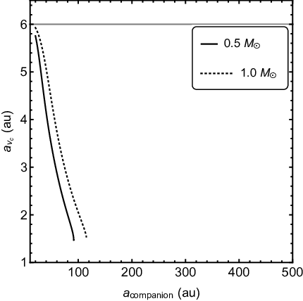
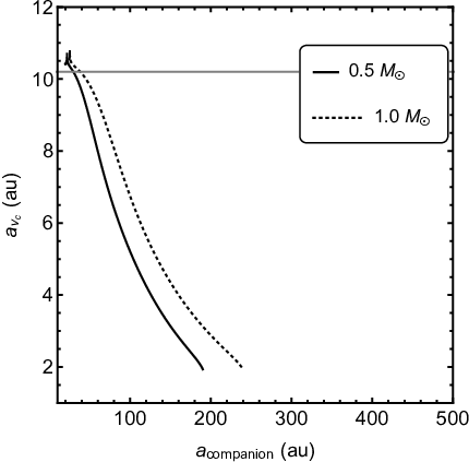
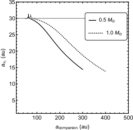
To identify how the secular resonance operates in a binary system, we use our analytic model described in Sec. 2.1. We replace the outer planetary companion with a stellar companion. In Fig. 9 we vary the mass and semi-major axis of the companion star for a white dwarf and calculate the location of the resulting secular resonance for three different semi-major axis values of the inner Jupiter mass planet. In Fig. 9, the location of the inner planet is (left panel), (middle panel), and (right panel). In each case, we vary the mass of the companion star as listed: (solid line) and (dashed). The middle panel corresponds to Jupiter at initially. In each panel, as the mass of the stellar companion increases, the location of the secular resonance can exist at a wider binary separations. Assuming that an asteroid belt is initially confined by the -like secular resonance, these models demonstrate that a variety of binary configurations may produce white dwarf pollution. Depending on the semi-major axis of the giant planet, this pollution mechanism (of secular perturbations) can support white dwarf pollution located in binaries with a binary separation . Note that since the Laplace-Lagrange equations are first order with respect to the orbital perturbations, this holds true only if this massive companion is very far way. We speculate that a white dwarf within a wide binary (i.e. ) can still become polluted not by the binary companion itself, but by perturbations driven by surviving planets orbiting the white dwarf, which follows the processes described in Section 2.1.
4 Conclusions
We have found that secular resonances, in particular the resonance, can be responsible for the presence of heavy elements in the atmosphere of white dwarfs. In the solar system, when the Earth becomes engulfed by the Sun as the latter leaves the main–sequence, the resonance is shifted outward. This mainly occurs because the free precession frequency of the asteroid is changed. This change in the location of the resonance causes previously stable asteroids to undergo secular resonant perturbations that lead to a higher rate of tidal disruptions close to the white dwarf. The resulting debris disc of heavy elements accretes onto the white dwarf, polluting the atmosphere. This mechanism can lead to white dwarf pollution for a large range of planetary system parameters including systems with two giant planets, or one planet and a binary star companion, assuming the presence of an asteroid belt initially confined by secular resonances, and the engulfment of an inner planet during the evolution of the star. From our numerical experiments, we expect the process of asteroid perturbations by secular resonances to last much longer than the white dwarf cooling age given a massive enough asteroid belt.
Debes et al. (2012) modeled the change in width of the 2:1 mean-motion resonance and found that the current mass of the asteroid belt would need to increase by a factor of in order for sufficient material to be accreted by the white dwarf by this mechanism alone. Frewen & Hansen (2014) later found that their model, that dealt with the accretion of a single planet, required a planetesimal disc to be a few thousand times larger than the asteroid belt. The estimate for the mass accretion rate in our model is on the lower end of the range of the observed accretion rates calculated by Koester et al. (2014) (Farihi, 2016, see also Figure 10 in). However, the asteroid belt in our Solar system is much less massive than other known warm debris discs. Knowing that there exist more massive planetesimal belts than our asteroid belt (Moro-Martín et al., 2010) gives encouraging evidence that secular resonances can potentially pollute white dwarfs.
While we don’t know with certainty whether the Sun will be polluted during its white dwarf stage due to asteroidal accretion, the analytical and numerical models used in this work do provide a possible mechanism for white dwarf pollution in exoplanetary systems. There is probably not just one mechanism that produces white dwarf pollution. Theoretically, our secular resonance model and the Debes et al. (2012) mean-motion resonance model could operate in a synergistic manner, allowing a larger fraction of asteroids to become tidally disrupted, but for exoplanetary systems resembling the Solar system, we expect that a higher flux of asteroids is influenced by secular perturbations rather than by mean-motion perturbations.
There are many known planetary system architectures in various databases including Kepler (Borucki et al., 2010; Borucki et al., 2011; Batalha et al., 2013), CoRoT (Auvergne et al., 2009), SuperWASP (Pollacco et al., 2006), and KELT (Pepper et al., 2007). In our pollution model we focus on exoplanetary systems that share strong features with the Solar system, including: two outer massive planets, an inner asteroid belt truncated by a secular resonance, an inner planet that is engulfed during the stellar evolution, and where all the bodies are on nearly circular and coplanar orbits. White dwarf pollution occurs in planetary systems that are vastly different from our Solar System. However, secular and mean-motion resonances are expected to sculpt the architecture of any asteroid belt in exoplanetary systems, so the global mechanisms presented in this article should be triggered (with more or less efficiency) in various planetary configurations.
Acknowledgements
We thank the anonymous referee for the helpful feedback which improved the quality of the manuscript. JLS also acknowledges support from a graduate fellowship from the Nevada Space Grant Consortium (NVSGC). All the simulations were submitted to the UNLV National Supercomputing Institute on the Cherry Creek cluster. We acknowledge support from NASA through grant NNX17AB96G.
References
- Aannestad et al. (1993) Aannestad P. A., Kenyon S. J., Hammond G. L., Sion E. M., 1993, AJ, 105, 1033
- Adams & Bloch (2013) Adams F. C., Bloch A. M., 2013, ApJ, 777, L30
- Armitage (2013) Armitage P. J., 2013, Astrophysics of Planet Formation
- Auvergne et al. (2009) Auvergne M., et al., 2009, A&A, 506, 411
- Barstow et al. (2014) Barstow M. A., Barstow J. K., Casewell S. L., Holberg J. B., Hubeny I., 2014, MNRAS, 440, 1607
- Batalha et al. (2013) Batalha N. M., et al., 2013, ApJS, 204, 24
- Bear & Soker (2013) Bear E., Soker N., 2013, New Astron., 19, 56
- Bonsor & Veras (2015) Bonsor A., Veras D., 2015, MNRAS, 454, 53
- Bonsor et al. (2017) Bonsor A., Farihi J., Wyatt M. C., van Lieshout R., 2017, MNRAS, 468, 154
- Borucki et al. (2010) Borucki W. J., et al., 2010, Science, 327, 977
- Borucki et al. (2011) Borucki W. J., et al., 2011, ApJ, 736, 19
- Bottke et al. (2000) Bottke Jr. W. F., Rubincam D. P., Burns J. A., 2000, Icarus, 145, 301
- Brouwer & van Woerkom (1950) Brouwer D., van Woerkom A. J. J., 1950, Astronomical papers prepared for the use of the American ephemeris and nautical almanac, v.13, pt.2, Washington : U.S. Govt. Print. Off., 1950., p. 81-107 : 29 cm., 13, 81
- Brož & Vokrouhlický (2008) Brož M., Vokrouhlický D., 2008, MNRAS, 390, 715
- Brown et al. (2017) Brown J. C., Veras D., Gänsicke B. T., 2017, MNRAS, 468, 1575
- Caiazzo & Heyl (2017) Caiazzo I., Heyl J. S., 2017, preprint, (arXiv:1702.07682)
- Chambers (1999) Chambers J. E., 1999, MNRAS, 304, 793
- Chrenko et al. (2015) Chrenko O., Brož M., Nesvorný D., Tsiganis K., Skoulidou D. K., 2015, MNRAS, 451, 2399
- Cottrell & Greenstein (1980) Cottrell P. L., Greenstein J. L., 1980, ApJ, 242, 195
- Davidsson (1999) Davidsson B. J. R., 1999, Icarus, 142, 525
- Deal et al. (2013) Deal M., Deheuvels S., Vauclair G., Vauclair S., Wachlin F. C., 2013, A&A, 557, L12
- Debes et al. (2012) Debes J. H., Walsh K. J., Stark C., 2012, ApJ, 747, 148
- Dermott & Murray (1983) Dermott S. F., Murray C. D., 1983, Nature, 301, 201
- Dohnanyi (1969) Dohnanyi J. S., 1969, J. Geophys. Res., 74, 2531
- Duncan & Lissauer (1998) Duncan M. J., Lissauer J. J., 1998, Icarus, 134, 303
- Falcon et al. (2010) Falcon R. E., Winget D. E., Montgomery M. H., Williams K. A., 2010, ApJ, 712, 585
- Farihi (2016) Farihi J., 2016, New Astron. Rev., 71, 9
- Farihi et al. (2009) Farihi J., Jura M., Zuckerman B., 2009, ApJ, 694, 805
- Farihi et al. (2010a) Farihi J., Barstow M. A., Redfield S., Dufour P., Hambly N. C., 2010a, MNRAS, 404, 2123
- Farihi et al. (2010b) Farihi J., Jura M., Lee J.-E., Zuckerman B., 2010b, ApJ, 714, 1386
- Farihi et al. (2012) Farihi J., Gänsicke B. T., Wyatt M. C., Girven J., Pringle J. E., King A. R., 2012, MNRAS, 424, 464
- Farihi et al. (2014) Farihi J., Wyatt M. C., Greaves J. S., Bonsor A., Sibthorpe B., Panić O., 2014, MNRAS, 444, 1821
- Fontaine & Michaud (1979) Fontaine G., Michaud G., 1979, ApJ, 231, 826
- Fontaine et al. (2001) Fontaine G., Brassard P., Bergeron P., 2001, PASP, 113, 409
- Frewen & Hansen (2014) Frewen S. F. N., Hansen B. M. S., 2014, MNRAS, 439, 2442
- Froeschle & Scholl (1986) Froeschle C., Scholl H., 1986, A&A, 166, 326
- Gänsicke et al. (2006) Gänsicke B. T., Marsh T. R., Southworth J., Rebassa-Mansergas A., 2006, Science, 314, 1908
- Gladman et al. (1997) Gladman B. J., et al., 1997, Science, 277, 197
- Granvik et al. (2017) Granvik M., Morbidelli A., Vokrouhlický D., Bottke W. F., Nesvorný D., Jedicke R., 2017, A&A, 598, A52
- Haghighipour & Winter (2016) Haghighipour N., Winter O. C., 2016, Celestial Mechanics and Dynamical Astronomy, 124, 235
- Hamers & Portegies Zwart (2016) Hamers A. S., Portegies Zwart S. F., 2016, MNRAS, 462, L84
- Horch et al. (2014) Horch E. P., Howell S. B., Everett M. E., Ciardi D. R., 2014, ApJ, 795, 60
- Ito & Malhotra (2006) Ito T., Malhotra R., 2006, Advances in Space Research, 38, 817
- Ito & Tanikawa (1999) Ito T., Tanikawa K., 1999, Icarus, 139, 336
- Izidoro et al. (2016) Izidoro A., Raymond S. N., Pierens A., Morbidelli A., Winter O. C., Nesvorny‘ D., 2016, ApJ, 833, 40
- Jura (2003) Jura M., 2003, ApJ, 584, L91
- Jura (2006) Jura M., 2006, ApJ, 653, 613
- Jura et al. (2009) Jura M., Muno M. P., Farihi J., Zuckerman B., 2009, ApJ, 699, 1473
- Kilic & Redfield (2007) Kilic M., Redfield S., 2007, ApJ, 660, 641
- Kilic et al. (2006) Kilic M., von Hippel T., Leggett S. K., Winget D. E., 2006, ApJ, 646, 474
- Klein et al. (2010) Klein B., Jura M., Koester D., Zuckerman B., Melis C., 2010, ApJ, 709, 950
- Knezevic et al. (1991) Knezevic Z., Milani A., Farinella P., Froeschle C., Froeschle C., 1991, Icarus, 93, 316
- Koester (2009) Koester D., 2009, A&A, 498, 517
- Koester & Wilken (2006) Koester D., Wilken D., 2006, A&A, 453, 1051
- Koester et al. (1982) Koester D., Weidemann V., Zeidler E. M., Vauclair G., 1982, A&A, 113, L13
- Koester et al. (1997) Koester D., Provencal J., Shipman H. L., 1997, A&A, 320, L57
- Koester et al. (2014) Koester D., Gänsicke B. T., Farihi J., 2014, A&A, 566, A34
- Krasinsky et al. (2002) Krasinsky G. A., Pitjeva E. V., Vasilyev M. V., Yagudina E. I., 2002, Icarus, 158, 98
- Lacombe et al. (1983) Lacombe P., Wesemael F., Fontaine G., Liebert J., 1983, ApJ, 272, 660
- Laskar (1988) Laskar J., 1988, A&A, 198, 341
- Laskar (1994) Laskar J., 1994, A&A, 287, L9
- Liebert et al. (2005) Liebert J., Bergeron P., Holberg J. B., 2005, ApJS, 156, 47
- Malhotra (2012) Malhotra R., 2012, Encyclopedia of Life Support Systems by UNESCO, 6, 55
- Malhotra et al. (1989) Malhotra R., Fox K., Murray C. D., Nicholson P. D., 1989, A&A, 221, 348
- McDonald & Zijlstra (2015) McDonald I., Zijlstra A. A., 2015, MNRAS, 448, 502
- Melis & Dufour (2017) Melis C., Dufour P., 2017, ApJ, 834, 1
- Melis et al. (2010) Melis C., Jura M., Albert L., Klein B., Zuckerman B., 2010, ApJ, 722, 1078
- Milani & Knezevic (1990) Milani A., Knezevic Z., 1990, Celestial Mechanics and Dynamical Astronomy, 49, 347
- Minton & Malhotra (2010) Minton D. A., Malhotra R., 2010, Icarus, 207, 744
- Minton & Malhotra (2011) Minton D. A., Malhotra R., 2011, ApJ, 732, 53
- Morbidelli & Gladman (1998) Morbidelli A., Gladman B., 1998, Meteoritics and Planetary Science, 33, 999
- Morbidelli & Henrard (1991) Morbidelli A., Henrard J., 1991, Celestial Mechanics and Dynamical Astronomy, 51, 169
- Morbidelli et al. (1995) Morbidelli A., Zappala V., Moons M., Cellino A., Gonczi R., 1995, Icarus, 118, 132
- Morbidelli et al. (2002) Morbidelli A., Bottke Jr. W. F., Froeschlé C., Michel P., 2002, Origin and Evolution of Near-Earth Objects. pp 409–422
- Moro-Martín et al. (2010) Moro-Martín A., Malhotra R., Bryden G., Rieke G. H., Su K. Y. L., Beichman C. A., Lawler S. M., 2010, ApJ, 717, 1123
- Murray & Dermott (2000) Murray C. D., Dermott S. F., 2000, Solar System Dynamics
- Murray & Holman (1997) Murray N., Holman M., 1997, AJ, 114, 1246
- Murray & Holman (1999) Murray N., Holman M., 1999, Science, 283, 1877
- Mustill & Villaver (2012) Mustill A. J., Villaver E., 2012, ApJ, 761, 121
- Nesvorný & Morbidelli (1998) Nesvorný D., Morbidelli A., 1998, AJ, 116, 3029
- Paquette et al. (1986) Paquette C., Pelletier C., Fontaine G., Michaud G., 1986, ApJS, 61, 197
- Payne et al. (2016) Payne M. J., Veras D., Holman M. J., Gänsicke B. T., 2016, MNRAS, 457, 217
- Payne et al. (2017) Payne M. J., Veras D., Gänsicke B. T., Holman M. J., 2017, MNRAS, 464, 2557
- Pepper et al. (2007) Pepper J., et al., 2007, PASP, 119, 923
- Petit et al. (2001) Petit J.-M., Morbidelli A., Chambers J., 2001, Icarus, 153, 338
- Petrovich & Muñoz (2017) Petrovich C., Muñoz D. J., 2017, ApJ, 834, 116
- Pollacco et al. (2006) Pollacco D. L., et al., 2006, PASP, 118, 1407
- Rasio et al. (1996) Rasio F. A., Tout C. A., Lubow S. H., Livio M., 1996, ApJ, 470, 1187
- Reach et al. (2005) Reach W. T., Kuchner M. J., von Hippel T., Burrows A., Mullally F., Kilic M., Winget D. E., 2005, ApJ, 635, L161
- Reimers (1977) Reimers D., 1977, A&A, 54, 485
- Rosenfield et al. (2014) Rosenfield P., et al., 2014, ApJ, 790, 22
- Rosenfield et al. (2016) Rosenfield P., Marigo P., Girardi L., Dalcanton J. J., Bressan A., Williams B. F., Dolphin A., 2016, ApJ, 822, 73
- Sackmann et al. (1993) Sackmann I.-J., Boothroyd A. I., Kraemer K. E., 1993, ApJ, 418, 457
- Schröder & Connon Smith (2008) Schröder K.-P., Connon Smith R., 2008, MNRAS, 386, 155
- Siess & Livio (1999) Siess L., Livio M., 1999, MNRAS, 308, 1133
- Smallwood et al. (2017) Smallwood J. L., Martin R. G., Lepp S., Livio M., 2017, MNRAS, in press
- Tremblay et al. (2016) Tremblay P.-E., Cummings J., Kalirai J. S., Gänsicke B. T., Gentile-Fusillo N., Raddi R., 2016, MNRAS, 461, 2100
- Vauclair et al. (1979) Vauclair G., Vauclair S., Greenstein J. L., 1979, A&A, 80, 79
- Vennes et al. (2010) Vennes S., Kawka A., Németh P., 2010, MNRAS, 404, L40
- Veras et al. (2011) Veras D., Wyatt M. C., Mustill A. J., Bonsor A., Eldridge J. J., 2011, MNRAS, 417, 2104
- Veras et al. (2013) Veras D., Hadjidemetriou J. D., Tout C. A., 2013, MNRAS, 435, 2416
- Veras et al. (2017) Veras D., Xu S., Rebassa-Mansergas A., 2017, preprint, (arXiv:1708.05391)
- Villaver & Livio (2007) Villaver E., Livio M., 2007, ApJ, 661, 1192
- Villaver & Livio (2009) Villaver E., Livio M., 2009, ApJ, 705, L81
- Villaver et al. (2014) Villaver E., Livio M., Mustill A. J., Siess L., 2014, ApJ, 794, 3
- Ward (1981) Ward W. R., 1981, Icarus, 47, 234
- Wyatt et al. (2014) Wyatt M. C., Farihi J., Pringle J. E., Bonsor A., 2014, MNRAS, 439, 3371
- Xu et al. (2018) Xu S., et al., 2018, MNRAS, 474, 4795
- Yoshikawa (1987) Yoshikawa M., 1987, Celestial Mechanics, 40, 233
- Zeidler-K.T. et al. (1986) Zeidler-K.T. E.-M., Weidemann V., Koester D., 1986, A&A, 155, 356
- Zuckerman et al. (2003) Zuckerman B., Koester D., Reid I. N., Hünsch M., 2003, ApJ, 596, 477
- Zuckerman et al. (2010) Zuckerman B., Melis C., Klein B., Koester D., Jura M., 2010, ApJ, 722, 725
- von Hippel et al. (2007) von Hippel T., Kuchner M. J., Kilic M., Mullally F., Reach W. T., 2007, ApJ, 662, 544