Tensor networks as path integral geometry
Abstract
In the context of a quantum critical spin chain whose low energy physics corresponds to a conformal field theory (CFT), it was recently demonstrated [A. Milsted G. Vidal, arXiv:1805.12524] that certain classes of tensor networks used for numerically describing the ground state of the spin chain can also be used to implement (discrete, approximate versions of) conformal transformations on the lattice. In the continuum, the same conformal transformations can be implemented through a CFT path integral on some curved spacetime. Based on this observation, in this paper we propose to interpret the tensor networks themselves as a path integrals on curved spacetime. This perspective assigns (a discrete, approximate version of) a geometry to the tensor network, namely that of the underlying curved spacetime.
The tensor network formalism [1, 2, 3, 4, 5, 6] allows for an efficient description of complex objects, such as many-body wavefunctions in quantum systems, and has in recent years become useful in a wide range of disciplines, including condensed matter [1, 2, 3], statistical mechanics [4, 5, 6], quantum gravity [7, 8, 9, 10, 11], quantum chemistry [12], quantum and classical information theory [13], and machine learning [14]. The geometry of a tensor network is of central importance from a computational viewpoint, since it largely determines our ability to perform efficient calculations. Moreover, the geometry also dictates the structure of possible correlations or dependencies within the complex object that the tensor network represents, e.g. the asymptotic scaling of entanglement entropy in many-body wavefunctions [15]. Finally, geometry is particularly important for the holographic interpretation of tensor networks in the context of the anti de Sitter / conformal field theory (AdS/CFT) correspondence [16]. There, tensor networks with hyperbolic geometry, such as the multi-scale entanglement renormalization ansatz (MERA) [2, 7, 8], the exact holographic mapping [9], the holographic error correction code [10] or the random tensor networks of Ref. [11], have been proposed as toy models for quantum gravity in AdS background. However, it is not always clear how to properly assign a geometry to a tensor network, or what that assignment really means. As a matter of fact, and rather confusingly, MERA has been speculated to realize two mutually incompatible geometries: the hyperbolic plane H2 [7] and de Sitter spacetime dS2 [8].
In this paper we propose a geometric characterization of a specific class of tensor networks, used to describe critical quantum spin chains, by arguing that they can be naturally interpreted as a CFT path integral on curved spacetime, see also [17, 18, 19]. Specifically, we consider two-dimensional tensor networks composed of three types of tensors: euclideons , disentanglers , and isometries (in absence of translation invariance, additional tensors known as smoothers are also included). Euclideons are obtained from an euclidean time evolution by the Hamiltonian of the critical quantum spin chain (or Boltzmann weights of a related two-dimensional statistical partition function), whereas disentanglers and isometries are MERA tensors optimized to represent the ground state of and can be obtained from the euclideons [20]. We recently demonstrated that strips of such tensor networks define linear maps that act on the low energy states of the quantum spin chain as conformal maps [21]. Each such conformal maps can be implemented in the continuum by a CFT path integral on a strip of some curved spacetime. By analogy, here we argue that we can then think of such tensor networks as describing (a discrete version of) a CFT euclidean path integral on a two-dimensional curved spacetime. In this way, we can assign a geometry to the tensor network: that of the underlying curved spacetime. However, a CFT path integral is invariant under local (Weyl) scale transformations. Hence requiring compatibility with a CFT path integral only determines the tensor network geometry up to a local scale factor . A unique geometry (up to a global scale factor, or choice of short distance cut-off ) can then be assigned by adding a second natural requirement, namely that the proper distance between nearest neighbor tensors be constant throughout the network. Accordingly, an euclideon anywhere in the network is seen to represent the euclidean path integral on a square patch of flat spacetime of size , whereas disentanglers and isometries implement space diffeomorphisms (local coordinate rescaling). A discrete curved geometry is then composed of microscopic square patches of flat euclidean spacetime connected non-trivially by such diffeomorphisms. Finally, as an example demonstrates, a systematically improved approximation to a continuous geometry is obtained by decreasing the cut-off .
Euclidean path integral as a linear map.— Let denote a two-dimensional euclidean spacetime where the spacetime manifold can be decomposed into ‘euclidean time’ slices , each topologically equivalent to a fixed one-dimensional ‘space’ manifold (see Fig. 1(a)). A generic metric in coordinates reads
| (1) |
where is a scale factor and and are general functions such that . A CFT is defined on this spacetime as usual in terms of a field (or set of fields) and its path integral
| (2) |
where and are the CFT action and lagrangian density. Crucial to our discussion, given a spacetime strip delimited by slices and for times and , the path integral restricted to defines a linear map in the CFT Hilbert space , see [22] for a review. Specifically, has matrix elements
| (3) |
where the field configurations are integrated over with and as boundary conditions. When the strip is thin, that is with (Fig. 1(b)), we can expand to linear order in . Its generator has two contributions
| (4) | |||||
| (5) |
that depend on the CFT hamiltonian and momentum densities and as well as on the metric in Eq. (1) through
| (6) |
Here is the generator of a non-uniform time evolution in , corresponding to a geometric deformation normal to the slice and proportional to ; generates instead a non-uniform space translation or local rescaling, corresponding to a reparametrization of space within according to , see Fig. 1(b).
Examples.— A generator of type is the Hamiltonian
| (7) |
which corresponds to and generates uniform time evolution in e.g. flat spacetime. Familiar generators include the momentum operator , which corresponds to and generates uniform space translations , and the dilation operator
| (8) |
which corresponds to and generates a uniform rescaling of the space coordinate. For later reference, we consider two simple geometries explicitly:
(i) The euclidean plane E2 has metric
| (9) |
implying and above. Therefore the path integral on a strip of with produces a linear map , generated by the Hamiltonian of Eq. (7), see Fig. 1(c).
(ii) The hyperbolic plane H2 with radius of curvature has metric in some conformal coordinates (with and ). With an alternative choice of coordinates and (with ), the same metric reads
| (10) |
or , , in Eq. (1); and in Eqs. (4)-(5). Thus in these coordinates the path integral on a thin strip of H2 implements a conformal map with generator
| (11) |
namely a linear combination of the Hamiltonian and the dilation operator in Eqs. (7)-(8), see Fig. 1(d).
Reconstructing the metric from the path integral.— Suppose now that, for all possible values of time , we have access to the infinitesimal conformal map obtained from the path integral on a thin strip at time . Do we have enough information to reconstruct the metric in Eq. (1)? By inspecting the generator and inverting Eq. (6), we can certainly recover and . This determines the conformal class of the metric, from which non-trivial information, such as its signature, can already be extracted [24]. However the method fails to provide the local scale factor in Eq. (1). This was to be expected, since the path integral of a CFT is essentially invariant under local (Weyl) rescaling [25]. In order to completely specify the geometry we must additionally provide the scale factor . Our proposed assignment of geometry to tensor networks (rule 1 below), will run into the same difficulty, which will be resolved by additionally specifying a scale factor (rule 2 below).
Tensor networks as geometry.— Consider now a critical quantum spin chain whose low energy, long-distance physics is described by a CFT. Ref. [21] recently argued that certain tensor networks implemented lattice versions of conformal transformations on the low energy states of the quantum spin chain. The simplest examples, see Figs. 2(a), are a single layer of euclideons , which implements an euclidean time evolution , and a double layer of disentanglers and isometries , which implements a global rescaling . More generally, one can combine euclideons, disentanglers, and isometries (and auxiliary tensors called smoothers [21]) into a single strip that is seen to implements a more general, finite linear map , where generates both non-uniform time evolution and local rescaling.
In this paper we propose to interpret this class of tensor networks as a path integral on a curved spacetime. Given a tensor network, we first decompose it as a product of layers or strips. For instance, the tensor network TN1 of Fig. 2(b) decomposes as the product of strips , whereas the tensor network TN2 of Fig. 2(d) decomposes as the product of strips . Each strip has two time slices as its boundaries. Each time slice corresponds to some discrete value of euclidean time and is equipped with a lattice whose sites are labeled by discrete space-time coordinates and correspond to the indices cut by that time slice, see e.g. Fig. 2(b). Lattice hosts the Hilbert space of a quantum spin chain, with each cut index representing a quantum spin. Then a strip of the tensor network implements a linear map between the spin chains at its bottom and top boundaries. We assign a geometry or metric to a tensor network by assigning a metric to each of its strips, following two rules.
Rule 1 (compatibility with path integral).— Let be the linear map implemented by a strip of a tensor network. Then the assigned strip geometry/metric should be such that the CFT path integral on it also produces the linear map .
For instance, since a layer of TN1 implements the linear map , with and in Eqs. (4)-(5) or and in Eq. (1), following rule 1 we assign the metric [23]
| (12) |
to tensor network TN1. In turn, each strip of tensor network TN2 implements the linear map [22], which equals for and generator . This generator is precisely in Eq. (11) for , corresponding to and , or and . Accordingly, rule 1 assigns to TN2 the metric [23]
| (13) |
We emphasize that rule 1 does not determine the scale factor in or , since any scale factor is compatible with the linear maps and implemented by a strip of these networks [25].
Rule 2 (constant lattice spacing).— The proper distance between any two equal-time, nearest neighbor lattice sites and is a constant for all discrete values of and across the tensor network.
For example, when applied to the tensor networks TN1 and TN2 above, rule 2 sets the scale factor of the metrics and in Eqs. (12)-(13) to . Temporarily choosing for simplicity, we then identify the geometry of these tensors networks as the Euclidean plane E2 in Eq. (9) and the hyperbolic plane H2 (with radius ) in Eq. (10), respectively.
It follows from the above examples that, as illustrated in Fig. 2(d), we can think of each euclideon as representing (a path integral on) a square patch of flat spacetime of size . In contrast, disentanglers and isometries do not represent a patch of geometry, but allow us to glue together the path integral on square pieces of flat spacetime (as given by the euclideons ) non-trivially into a path integral on some curved spacetime, such as H2.
Refinement limit.— Given a curved spacetime with metric as a target, we can use a sequence of tensor networks with decreasing lattice spacing to systematically obtain a finer approximation to the CFT path integral on the target continuous spacetime. As an example, consider a topological cylinder , where each time slice for is now a circle of unit perimeter and, thus parameterized, the space coordinate is periodic, and let the metric be as in Eq. (1) with , and , where . Fig. 3(d) shows a sequence of discrete approximations to a periodic strip with boundaries and , which has an -dependent width (as measured in proper euclidean time) given by . In the continuum, the CFT path integral on this strip implements a finite linear map generated by where (non-uniform euclidean time evolution) dominates and (space diffeomorphism) is only a small correction [22]. On the lattice, the tensor networks act on the low energy states of a sequence of periodic quantum spin chain of size , where . As we decrease , the discrete profile of euclideons approximates better the continuous function , suggesting a better approximation to the continuous strip geometry. Indeed, the linear map implemented by the tensor network is seen to better approximate the conformal map obtained through the path integral in the continuum [22].
(a)
(b)
Discussion.— In this paper we have proposed how to assign geometries to a class of tensor networks describing quantum critical spin chains. Our main contribution is rule 1 above, which requires that the linear map implemented by a strip of the network should be compatible with the linear map implemented in the continuum by the CFT path integral on a strip of the assigned geometry. The second requirement, namely that the lattice spacing correspond to a constant distance throughout the network (rule 2 above), has also been used in most previous proposals to assign geometries to tensor networks [7, 8, 9, 10, 11, 17, 18, 19]. Several remarks are in order. (i) While rule 2 conveniently allowed us to assign a single length scale throughout the tensor network, the tensor network formalism can also be used to describe a CFT on a lattice with inhomogeneous lattice spacing , in which case rule 2 is replaced with the choice of scale factor , see e.g. Refs. [31, 32]. (ii) By considering lorentzions (such that a layer of lorentzions implements a map ) instead of euclideons , our present proposal extends also to 2d spacetime geometries with lorentzian signature [32]. (iii) Finally, a similar geometric assignment is possible for tensor networks describing lattice models whose low energy physics correspond instead to a massive quantum field theory. In this case the tensors in the network (euclideons, disentanglers and isometries) are no longer scale-invariant but seen to depend explicitly on the UV cut-off scale [32].
A main motivation for this work was to develop natural criteria to assign a geometry to the MERA. As discussed in Ref. [24], from the perspective of the path integral advocated here, MERA corresponds to a degenerate geometry (the metric has zero determinant) which is therefore neither the hyperbolic plane H2 [7] nor de Sitter spacetime dS2 [8]. However, the MERA tensor network is also shown to admit euclidean and lorentzian extensions that correspond to a path integral in both H2 and dS1,1, thus realizing the scenarios described in Refs. [7] and [8].
Acknowledgments. We thank Bartlomiej Czech, Pawel Caputa, William Donnelly, Davide Gaiotto, Qi Hu, Lampros Lamprou, Juan Maldacena, David Mateos, Samuel McCandlish, Rob Myers, James Sully, Vasudev Shyam, Tadashi Takayanagi, and Xiao-liang Qi for fruitful discussions and feedback. The authors acknowledge support by the Simons Foundation (Many Electron Collaboration), by NSERC (discovery grant), and by Compute Canada. Research at Research at Perimeter Institute is supported by the Government of Canada through the Department of Innovation, Science and Economic Development Canada and by the Province of Ontario through the Ministry of Research, Innovation and Science.
References
- [1] M. Fannes, B. Nachtergaele, and R. F. Werner, Finitely correlated states on quantum spin chains, Math. Phys. 144, 443 (1992). S.R. White, Density matrix formulation for quantum renormalization groups, Phys. Rev. Lett. 69, 2863 (1992). U. Schollwöck, The density-matrix renormalization group in the age of matrix product states, Annals of Physics 326, 96 (2011), arXiv:1008.3477.
- [2] G. Vidal, Entanglement renormalization, Phys. Rev. Let. 99, 220405 (2007), arXiv: cond-mat/0512165; A class of quantum many-body states that can be efficiently simulated, Phys. Rev. Lett. 101, 110501 (2008), arXiv: quant-ph/0610099.
- [3] F. Verstraete, and J. I. Cirac, Renormalization algorithms for Quantum-Many Body Systems in two and higher dimensions, arXiv:cond-mat/0407066v1 (2004). G. Sierra and M.A. Martin-Delgado, The Density Matrix Renormalization Group, Quantum Groups and Conformal Field Theory, arXiv:cond-mat/9811170v3 (1998). Y. Nishio, N. Maeshima, A. Gendiar, and T. Nishino, Tensor Product Variational Formulation for Quantum Systems, arXiv:condmat/0401115 (2004).
- [4] T. Nishino, Density Matrix Renormalization Group Method for 2D Classical Models, J. Phys. Soc. Jpn. 64, 3598-3601(1995). T. Nishino, K. Okunishi, Corner Transfer Matrix Renormalization Group Method, J. Phys. Soc. Jpn. 65, 891 (1996) T. Nishino and K. Okunishi, A Density Matrix Algorithm for 3D Classical Models, J. Phys. Soc. Jpn., 67, 3066 (1998).
- [5] M. Levin, C.P. Nave, Tensor renormalization group approach to 2D classical lattice models, Phys. Rev. Lett. 99, 120601 (2007). Z.-C. Gu and X.-G. Wen, Tensor-Entanglement-Filtering Renormalization Approach and Symmetry Protected Topological Order, Phys. Rev. B80, 155131 (2009), arXiv:0903.1069. Z. Y. Xie, H. C. Jiang, Q. N. Chen, Z. Y. Weng, and T. Xiang, Second Renormalization of Tensor-Network States, Phys. Rev. Lett. 103, 160601 (2009), arXiv:0809.0182.
- [6] G. Evenbly, G. Vidal, Tensor network renormalization, Phys. Rev. Lett. 115 (18), 180405 (2015), arXiv:1412.0732. S. Yang, Z.-C. Gu, and X.-G. Wen, Loop Optimization for Tensor Network Renormalization, Phys. Rev. Lett. 118, 110504 (2017), arXiv:1512.04938. M. Bal, M. Marien, J. Haegeman, and F. Verstraete, Renormalization group flows of Hamiltonians using tensor networks, Phys. Rev. Lett. 118, 250602 (2017), arXiv:1703.00365. M. Hauru, C. Delcamp, S. Mizera, Renormalization of tensor networks using graph independent local truncations, Phys. Rev. B 97, 045111 (2018), arXiv:1709.07460.
- [7] B. Swingle, Entanglement Renormalization and Holography, Phys. Rev. D 86, 065007 (2012), arXiv:0905.1317. B. Swingle, Constructing holographic spacetimes using entanglement renormalization, arXiv:1209.3304.
- [8] C. Beny, Causal structure of the entanglement renormalization ansatz, New J. Phys. 15 (2013) 023020, arXiv:1110.4872. B. Czech, L. Lamprou, S.l McCandlish, and J. Sully, Tensor Networks from Kinematic Space, 10.1007/JHEP07 (2016) 100, arXiv:1512.01548. R.S. Kunkolienkar, K. Banerjee, Towards a dS/MERA correspondence, Int. J. Mod. Phys. D 26, 1750143 (2017), arxiv:1611.08581. N. Bao, C. Cao, S. M. Carroll, A. Chatwin-Davies. De Sitter space as a tensor network: Cosmic no-hair, complementarity, and complexity, Phys. Rev. D 96, 123536 (2017), arXiv:1709.03513.
- [9] X.-L. Qi, Exact holographic mapping and emergent spacetime geometry, arXiv:1309.6282. C. H. Lee, X.-L. Qi Exact holographic mapping in free fermion systems Phys. Rev. B 93,035112 (2016), arXiv:1503.08592.
- [10] F. Pastawski, B. Yoshida, D. Harlow, J. Preskill, Holographic quantum error-correcting codes: Toy models for the bulk/boundary correspondence JHEP 06 (2015) 149, arXiv:1503.06237.
- [11] P. Hayden, S. Nezami, X.-L. Qi, N. Thomas, M. Walter, Z. Yang, Holographic duality from random tensor networks, JHEP 11 (2016) 009, arXiv:1601.01694. X.-L. Qi, Z. Yang, Space-time random tensor networks and holographic duality, arXiv:1801.05289.
- [12] S. R. White and R. L. Martin, Ab initio quantum chemistry using the density matrix renormalization group, J. Chem. Phys. 110, 4127 (1999). G. K.-L. Chan, M. Head-Gordon, Highly correlated calculations with a polynomial cost algorithm: A study of the density matrix renormalization group, J. Chem. Phys. 116, 4462 (2002).
- [13] A. J. Ferris, D. Poulin Tensor Networks and Quantum Error Correction, Phys. Rev. Lett. 113, 030501(2014), arXiv:1312.4578. AJ Ferris, D Poulin Branching MERA codes: A natural extension of classical and quantum polar codes Information Theory (ISIT), 2014 IEEE International Symposium on, 1081-1085.
- [14] C. Beny, Deep learning and the renormalization group, arXiv:1301.3124 E.M. Stoudenmire, D.J. Schwab Supervised Learning with Quantum-Inspired Tensor Networks, Advances in Neural Information Processing Systems 29, 4799 (2016), arXiv:1605.05775. Y. Levine, O. Sharir, N. Cohen, A. Shashua, Bridging Many-Body Quantum Physics and Deep Learning via Tensor Networks, arXiv:1803.09780.
- [15] G. Evenbly, G. Vidal, Tensor network states and geometry, J. Stat. Phys. (2011) 145:891-918, arXiv:1106.1082.
- [16] J.M. Maldacena, The Large N Limit of Superconformal Field Theories and Supergravity, Adv. Theor. Math. Phys. 2:231-252 (1998), arXiv:hep-th/9711200. S. S. Gubser, I. R. Klebanov, and A. M. Polyakov, Gauge Theory Correlators from Non-Critical String Theory, Phys. Lett. B 428, 105 (1998), arXiv:hep-th/9802109. E. Witten, Anti De Sitter Space And Holography, Adv. Theor. Math. Phys. 2, 253 (1998), arXiv:hep-th/9802150.
- [17] M. Miyaji, T. Takayanagi, K. Watanabe, From Path Integrals to Tensor Networks for AdS/CFT, Phys. Rev. D 95, 066004 (2017), arXiv:1609.04645. P. Caputa, N. Kundu, M. Miyaji, T. Takayanagi, K. Watanabe, Anti-de Sitter Space from Optimization of Path Integrals in Conformal Field Theories, Phys. Rev. Lett. 119, 071602 (2017), arXiv:1703.00456. P. Caputa, N. Kundu, M. Miyaji, T. Takayanagi, K. Watanabe, Liouville Action as Path-Integral Complexity: From Continuous Tensor Networks to AdS/CFT, JHEP 11(2017)097, arXiv:1706.07056.
- [18] B. Czech, Einstein’s equations from Varying Complexity, Phys. Rev. Lett. 120, 031601 (2018), arXiv:1706.00965.
- [19] G. Evenbly, G. Vidal Local scale transformations on the lattice with tensor network renormalization, Phys. Rev. Lett. 116, 040401 (2016), arXiv:1510.00689.
- [20] G. Evenbly, G. Vidal Tensor network renormalization yields the multi-scale entanglement renormalization ansatz, Phys. Rev. Lett. 115, 200401 (2015), arXiv:1502.05385
- [21] A. Milsted, G. Vidal, Tensor networks as conformal transformations, arXiv:1805.12524.
- [22] See Supplemental Material for further details.
- [23] A finite conformal map may in general have alternative descriptions of the form in terms of a different generator (or even as a path-ordered exponential for a time dependent generator ), each leading to an alternative geometry. This is expected: in a discrete network we cannot resolve the geometry at distances shorter than the spacing between nearest neighbour tensors. However, by analysing a very long strip, the linear map becomes infinitesimal, , and we can then resolve these ambiguities by identifying the unique generator . For instance, a periodic layer made of euclideons implements the map , where . Thus, for large its action on low energy states is , where is the scaling dimension of the state. We can then unambiguously assign the generator (and thus the metric in Eq. (12)) to .
- [24] A. Milsted, G. Vidal, Geometric interpretation of the multi-scale entanglement renormalization ansatz, in preparation.
- [25] In a CFT, the linear map implemented by the path integral is sensitive to a Weyl rescaling through a multiplicative constant given by the exponential of the Liouville action [17, 18]. This multiplicative constant, which does not affect correlation functions (since the same factor appears in the partition function with and without field insertions), is not reproduced by the tensor network [19] and will be ignored in our current discussion.
- [26] A. A. Belavin, A. M. Polyakov, and A. B. Zamolodchikov, Infinite conformal symmetry in two-dimensional quantum field theory, Nucl. Phys. B 241, 333 (1984). D. Friedan, Z. Qiu, and S. Shenker, Conformal Invariance, Unitarity, and Critical Exponents in Two Dimensions, Phys. Rev. Lett. 52, 1575 (1984).
- [27] F. Verstraete and J. I. Cirac, Matrix product states represent ground states faithfully, Phys. Rev. B 73, 094423 (2006).
- [28] S. Rommer and S. Östlund, Class of ansatz wave functions for one-dimensional spin systems and their relation to the density matrix renormalization group, Phys. Rev. B 55, 2164 (1997). F. Verstraete, D. Porras, and J. I. Cirac, DMRG and periodic boundary conditions: a quantum information perspective, Phys. Rev. Lett. 93, 227205 (2004), cond-mat/0404706. B. Pirvu, F. Verstraete, and G. Vidal, Exploiting translational invariance in matrix product state simulations of spin chains with periodic boundary conditions, Phys. Rev. B 83, 125104 (2011). B. Pirvu, J. Haegeman, and F. Verstraete, A matrix product state based algorithm for determining dispersion relations of quantum spin chains with periodic boundary conditions, Phys. Rev. B 85, (2012), arXiv:1103.2735.
- [29] Y. Zou, A. Milsted, G. Vidal, Conformal data and renormalization group flow in critical quantum spin chains using periodic uniform matrix product states, arXiv:1710.05397.
- [30] W. M. Koo and H. Saleur, Representations of the Virasoro algebra from lattice models, Nucl. Phys. B 426, 459 (1994), arXiv:hep-th/9312156. A. Milsted, G. Vidal Extraction of conformal data in critical quantum spin chains using the Koo-Saleur formula, Phys. Rev. B 96 (24), 245105 (2017), arXiv:1706.01436.
- [31] B. Czech, G. Evenbly, L. Lamprou, S. McCandlish, X.-L. Qi, J. Sully, G. Vidal, A tensor network quotient takes the vacuum to the thermal state, Phys. Rev. B 94, 085101 (2016), arXiv:1510.07637.
- [32] A. Lewis et al., Tensor networks for quantum field theories in curved spacetime, in preparation.
I Appendix: 2d geometry as linear maps between time slices
Sections I.1 to I.8 we provide a detailed derivation of Eqs. 1-6 of the main text. This is standard material that can be found scattered in most graduate-level QFT/CFT books. We compiled this material together in uniform notation for completeness. These sections do not contain original research.
I.1 Slicing
We consider a 2d euclidean spacetime where, for simplicity, the manifold can be decomposed into non-overlapping, one-dimensional slices
| (14) |
and where each slice is topologically equivalent to a fixed one-dimensional manifold , so that topologically we have . We will think of as a space-like surface and of as labeling euclidean time. A concrete example would be a topological cylinder, where the space-like surface is a circle S1.
We choose coordinates on such that, by construction, the euclidean time is constant on each slice . In these coordinates the metric reads
Here we have explicitly extracted a scale factor for later convenience. Recall that the euclidean metric is positive defined, so that the determinant is positive, that is for all . The inverse metric reads
In the tangent space of at , let
| (27) |
be the vector such that, for small , maps each point in slice into a corresponding point in slice (that is, without changing the coordinate ),
| (28) |
and let be the unit normal vector to ,
| (29) | |||||
| (30) |
or
| (31) | |||||
| (32) |
where the normalization above was fixed by the condition . We will be interested in the scalar products and , which read
| (33) | |||||
| (34) |

I.2 Auxiliary conformal coordinates
Next we introduce an auxiliary set of conformal coordinates such that they coincide with on the time slice , that is, when , see Fig. 4. As in any set of conformal coordinates, the metric expressed in the coordinates is proportional to the identity,
| (35) |
and
| (36) |
Moreover, by construction the scale factor coincides with on the slice ,
| (37) |
Let
| (38) |
be the transition vector between slices and , Eq. (27), when expressed in the conformal coordinates , see Figs. 4-5. In these coordinates the unit normal vector in Eq. (29)-(32) now reads
| (39) |
The scalar products and in Eq. (33)-(34), which are invariant under a change of coordinates, now read
| (40) | |||||
| (41) |
We thus conclude, comparing Eqs. (33)-(34) with Eqs. (40)-(41), that
| (42) |
or, equivalently,
| (43) |

I.3 Path integral and transition amplitudes
On the euclidean spacetime () parameterized by we define a local QFT, characterized by a field (possibly representing a set of several fields) and the path integral
| (44) |
where is an integral over field configurations and is the action of a given field configuration , that is
| (45) |
where is a local lagrangian density.
Given two times and , with , let denote the strip of geometry that has the corresponding slices and as its boundaries. Then the path integral on with the field boundary conditions
| (46) |
defines a transition amplitude
| (47) |
I.4 Hilbert space and linear maps
Given a slice , we define the Hilbert space in terms of a basis of vectors , where each such vector corresponds to a field configuration on . Further, given the two slices and , we identify basis vectors on the corresponding Hilbert spaces and through
| (48) |
This identification between states in the Hilbert space, which depends on the choice of spatial coordinate on and , allows us to consider a single Hilbert space for all slices .
We then use the transition amplitude in Eq. (47) to define a linear map with matrix elements
| (49) |
Through the above identification, it becomes a linear map .
I.5 Generator of the linear map for a thin strip
When for a small , is a thin strip and we can expand the linear map to linear order in ,
| (50) |
As reviewed in the derivation below, can be written in terms of the euclidean stress tensor as
Here is the proper length attached to an infinitesimal of the space coordinate , is the unit normal vector of at position , and is the transition vector such that maps points in to points in without changing the value of the space coordinate . Given that both and transform as scalars under a change of coordinates, we can evaluate their product in the auxiliary conformal coordinates , which are adjusted to coincide with at , that is, such that for . We then find
| (51) | |||||
| (52) | |||||
| (53) |
where and are the components of in Eq. (38), and in these expressions .
We proceed by specializing to a CFT. In conformal coordinates, the stress tensor always has the same components and (up to an additive constant due to the conformal anomaly, which for the purposes of this work we can ignore, see [25]), where and are the euclidean energy and momentum densities. In terms of the more conventional lorentzian energy and momentum densities and (see free boson example below), we arrive to
| (54) | |||||
| (55) |
where we have split the generator into two contributions
| (56) | |||||
| (57) |
that generate non-uniform time and space translations, respectively.
I.6 Stress tensor and Ward identity
In our derivation below, the euclidean stress tensor plays an important role. It can be defined in two alternative ways. First, using Noether’s theorem, as a pair of classically conserved currents (corresponding to the invariance of the action under time and space translations). Second, as characterizing the variations of the action under changes of the metric.
Consider an infinitesimal change of coordinates of the form
| (58) |
and a new field through
| (59) |
We notice that
| (60) |
and therefore the determinant of the Jacobian reads
| (61) |
whereas
| (62) | |||||
| (63) | |||||
| (64) | |||||
| (65) |
Given a field configuration , let us rewrite its action as
| (66) | |||||
| (67) | |||||
| (68) | |||||
| (69) | |||||
| (70) | |||||
| (71) | |||||
| (72) |
where (66) is the definition, in (67) we changed coordinates, in (68) we simply renamed the coordinates as (since they are integration variables), in (69) we expanded the Lagrangian according to
| (73) |
in (70) we separated a first term independent of and a second term that collects all contributions linear in (the contribution linear in must vanish since the action is invariant under uniform time and space translations), in (71) we identified the first term as the original action evaluated on the new field configuration and the second term as an integral of times the euclidean stress tensor
| (74) |
evaluated on the field configuration (or on the field , up to corrections that are higher order in ) and, finally, in (72) we used integration by parts in the second term. Noether’s theorem applied to invariance of the action under uniform time-space translations implies that the stress tensor is conserved
| (75) |
when evaluated on classical field configurations , that is, field configurations that extremize the action functional (and thus obey the classical equations of motion).
Alternatively, we could first rewrite the action functional in an explicitly covariant form by introducing the metric ,
| (76) |
and then define the euclidean stress tensor in terms of the variations of the action under changes of the metric (which it is then set back to being flat, that is )
| (77) |
see below the case of a free boson as an example.
Let us now consider the path integral with
| (78) |
where is the action functional of Eq. (66) and could be a single local insertion , e.g. or, more generally, a sequence of such local insertions at points . Let us rewrite this expression considering the above infinitesimal change of coordinates (58) were we will assume for simplicity that the coordinates do not change (that is, vanishes) in a finite neighborhood of the location of each insertion in . Then we have
| (79) | |||||
| (80) | |||||
| (81) | |||||
In (80) we assumed as customary that the functional integration measure is invariant under the field transformation, that is , and used Eqs. (66)-(72). Then in (81) we separate a first term independent of from a second term that collects all linear order contributions in . Now we notice that the field is an integration variable and we can change its name to , which makes manifest that this first term is equal to . Therefore we arrive to
| (82) |
which is valid for all (with the above restriction) and thus implies that
| (83) |
for all which does not coincide with the insertion(s) , that is .
I.7 Infinitesimal evolution of the wavefunctional
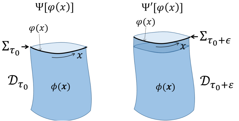
Consider the wavefunctional on the time slice at time , defined through a path integral on the domain , consisting of all times , as
| (86) | |||||
Here the path integral is over field configurations for and such that they coincide with at the boundary of , that is . The action functional now reads
| (87) |
By changing the insertion(s) , we could obtain a different wavefunctional . Notice that the wavefunctional corresponds to a vector in the Hilbert space ,
| (88) |
Our goal is to evolve the wavefunctional from time to time using the path integral in the intermediate strip, which will produce a new wavefunctional
| (91) | |||||
That is, now the path integral is over field configurations for and such that they coincide with at the boundary of , with
| (92) |
Notice that the insertion is the same as before. The new wavefunctional corresponds to a vector in the Hilbert space , but with the identification of Eq. (48) we can think of both states and as belonging to the same Hilbert space .
To compute the evolution from to we will consider a change of coordinates as in Eq. (58) where is a smooth, infinitesimal function of such that: (i) it is only non-zero in a small neighborhood of the boundary of that does not contain the positions of the insertions . (ii) when acting on time slice , the coordinate change maps each point into the point of the time slice , that is
| (93) |
where had been introduced in Eq. (27).
We can now proceed to define a new field through as before, and study how the action functional changes under the coordinate and field transformations, as we did previously. This time, however, we must account for the change in the boundary conditions. Let be a field configuration on that fulfills the boundary conditions on . Its action reads
| (94) | |||||
| (95) | |||||
| (96) | |||||
| (97) | |||||
| (98) |
In going from (94) to (95) we have explicitly accounted for the change in the integration domain. In the next step we simply relabeled the integration coordinates . In (96) we separated a first term which only depends on through the domain of integration of , and a second term that collects all contributions linear in (the derivative of) (notice that we have reset the integration limit of to , but introducing corrections that are quadratic in ). Then in (98) we have identified the first term with the action of the field configuration , which is defined on the domain and fulfills the boundary conditions , and the second term as an integral of the stress tensor.
Finally, we are ready to apply the same coordinate and field transformations to the path integral expression of the wavefunctional . We obtain:
| (99) | |||||
| (100) | |||||
| (101) |
Notice that above it is crucial that the insertions are not affected by the change of coordinates. We also note that, since in this last expression the field is an integration variable, we can rename it . It then follows that
| (102) | |||
| (103) | |||
In (102) we have used the Ward identity in Eq. (83) to extend the domain of the partial derivative to include the stress tensor, whereas in (103) we have identified the first term in (102) with the new wavefunctional and we have applied Stokes’ theorem (namely ) to the second term in (102). After introducing the field operator and its conjugate momentum on , and making the replacements and , Eqs. (102)-(103) can be seen to be equivalent to , that is
| (104) |
where
| (105) | |||||
| (106) |
I.8 Example: free boson QFT in flat spacetime
Here we briefly compare the lorentzian and euclidean QFT formalisms, with a free boson as a concrete example. We temporarily use subscripts L and E to differentiate between the two cases.
Recall that in a 2d lorentzian QFT with bosonic field , where are cartesian coordinates on Minkowski space-time with metric diag, the path integral and the action functional read
| (107) | |||||
| (108) |
where is the lagrangian. Invariance of the action under space-time translations leads to the classically conserved stress tensor ,
| (109) |
with energy and momentum densities and , and classically conserved charges and given by
| (110) | |||||
| (111) |
For a massive free boson we have
| (112) | |||||
| (113) | |||||
| (114) | |||||
| (115) |
Let us now consider, as we did in most of this paper, a 2d euclidean QFT with with bosonic field , where now are cartesian coordinates on the euclidean plane with metric diag. The path integral and the action functional read
| (116) | |||||
| (117) |
where is the lagrangian. Invariance under spacetime translations leads to the classically conserved stress tensor
| (118) |
with energy and momentum densities and , and classically conserved charges and given by
| (119) | |||||
| (120) |
For a massive free boson we have
| (121) | |||||
| (122) | |||||
| (123) | |||||
| (124) |
Notice that the euclidean lagrangian can be obtained from the lorentzian lagrangian by replacing with and adding a an overall minus sign, that is
In defining operators in the Hilbert space or at time or , besides the field operator we also introduce its conjugate momentum , which is the same in lorentzian and euclidean QFT and is defined as
| (125) |
For instance, in the free boson QFT considered above, we have
| (126) |
Then, remaining with the free boson, the hamiltonian and momentum densities and and the hamiltonian and momentum operators and , which are the generators of unitary transformations (in the Hilbert space ) corresponding to time and space translations, are obtained from , , and by replacing and , and thus read
| (127) | |||||
| (128) | |||||
| (129) | |||||
| (130) |
The euclidean Hamiltonian and momentum densities the hamiltonian and momentum densities and , and hamiltonian and momentum operators and ,which are the generators of euclidean time evolution and of space translations in the same Hilbert space, are obtained instead from , , and by replacing and . Thus they read
| (131) | |||||
| (132) | |||||
| (133) | |||||
| (134) |
We conclude that lorentzian and euclidean densities/generators are related to each other as
| (135) | |||||
| (136) |
This is consistent with the Heisenberg picture operator evolutions
| (137) | |||||
| (138) |
II Appendix: Refining a tensor network toward a strip of continuous path integral
In this section we describe a sequence of tensor networks, illustrated in Fig. 7, whose actions as linear maps, on the low-energy states of a critical spin chain, approach the action of a strip of continuous euclidean-time path integral. For a CFT, the latter can be viewed as a conformal transformation whose matrix elements we can compute perturbatively in the thickness of the strip. We are therefore able to confirm that the tensor network maps are approaching the correct continuum limit by comparing their matrix elements with equivalent matrix elements of the conformal transformation.
(a)
(b)
(c)
Each tensor network is designed to implement nonuniform euclidean time evolution on a flat cylinder, with the amount of euclidean time evolution at each point in space approximating, in the discretuum, the continuous function
| (139) |
where and . We carry out computations for the case , for which the tensor networks are those illustrated in Fig. 7 in the main text. Each tensor network has a different effective lattice spacing, with the sequence corresponding to a refinement of . As such we expect the action of the linear maps implemented by these tensor networks to approach that of a corresponding nonuniform strip of euclidean-time path integral. We now examine how to compute matrix elements of the latter.
II.1 CFT matrix elements
Given a CFT Hilbert space , associated with timeslices and of a CFT euclidean time path integral on a manifold , we wish to compute the action of the linear map given by the strip of path integral enclosed by and . We specialize to the particular case of a flat cylinder with coordinates , and metric
| (140) |
and where the timeslices are defined by
| (141) | ||||
| (142) |
where is defined in Eq. (139). Given an action for the path integral, this is enough to define the linear map . Note, however, that the two timeslices have different proper lengths. In particular, differences in do not equal the corresponding proper distances on . If we compare states on the timeslices using the common coordinate, we are implicitly applying a local rescaling – a Weyl transformation – that matches up the internal geometry of one timeslice with that of the other. The effective map is thus . On the CFT Hilbert space, acts as a multiple of the identity and can be ignored, as discussed in the main text.
As discussed in the main text, the matrix elements for eigenstates of the CFT Hamiltonian on are those of an appropriately chosen conformal transformation
| (143) |
where the generator can be expressed in terms of chiral and anti-chiral Virasoro generators
| (144) |
In the following, we fist show how to determine the generator of the conformal coordinate transformation in terms of conformal generators obeying the Witt algebra. We then obtain the generator of the corresponding transformation on the CFT Hilbert space by replacing elements of the Witt algebra with elements of the Virasoro algebra. Given irreducible representations of the Virasoro algebra belonging to a particular CFT, we apply the Virasoro commutator to compute, perturbatively, the desired matrix elements of .
II.1.1 Conformal coordinate transformation
So that we may ultimately define, for the linear map , a corresponding conformal transformation in terms of Virasoro generators, we need to work with a set of conformal coordinates that coincide with the coordinates on . Fortunately, the coordinates are already conformal (indeed, the metric in these coordinates is flat). We can thus proceed to define a conformal coordinate transformation that, viewed as an active transformation, maps onto :
| (145) |
A conformal coordinate transformation that achieves this is given by the holomorphic function
| (146) |
where and . In the new coordinates, the timeslice is specified by
| (147) |
Let us briefly consider the metric in the coordinates: Given that are conformal coordinates, and that are related to by a conformal transformation (Eq. (146)), the metric of Eq. (140) must take the form
| (148) |
for some function , which we know to be nontrivial, since the proper distance along . An example of a Weyl transformation that restores the feature that measures the proper distance along is
| (149) |
Returning to the conformal coordinate transformation of Eq. (146), the next step is to find its generator. The generators of conformal coordinate transformations on the flat cylinder of unit radius are
| (150) |
and can be seen to realize the Witt algebra
| (151) |
Writing the transformation of Eq. (146) as
| (152) |
so that , we may determine the generator
| (153) |
perturbatively in the parameter of Eq. (139). We expand the exponential in Eq. (152), and seek so that for some chosen integer . For , this results in the generator coefficients
| (154) |
leading to the generator
| (155) |
so that
| (156) |
which matches Eq. (146) up to corrections. For , (shown in Fig. 3) the required coefficients are
| (157) | ||||
| (158) | ||||
| (159) | ||||
| (160) | ||||
| (161) | ||||
| (162) | ||||
| (163) | ||||
| (164) | ||||
| (165) | ||||
| (166) |
where all not appearing above are set to zero.
Note that the generator of the conjugate coordinate transformation
| (167) |
is simply
| (168) |
II.1.2 Conformal transformation on the CFT Hilbert space
We now proceed to quantize the conformal coordinate transformation of Eq. (146). The quantized version of the Witt algebra is the Virasoro algebra (a central extension of the former). On a timeslice, such as , of the flat Euclidean cylinder, two commuting copies of the Virasoro algebra are realized
| (169) | |||||
| (170) | |||||
| (171) |
where is the central charge and the chiral and anti-chiral Virasoro generators and are the quantum equivalents of the Witt generators and . The quantization of a conformal transformation is therefore, roughly, the replacement of Witt generators with Virasoro generators in Eq. (152). More precisely, we define the quantized transformation to be
| (172) |
with the chiral and anti-chiral generators
| (173) | ||||
| (174) |
The coefficients are those defined in the previous section for the coordinate transformation.
II.1.3 Computation of matrix elements
To compute matrix elements of , we first expand the exponential in Eq. (172) to the same order used above to find the generator coefficients . Matrix elements of can then be approximately computed in terms of matrix elements of the various products of Virasoro generators in the expansion:
| (175) |
We now explain how to compute matrix elements of arbitrary products of Virasoro generators in terms of eigenstates of the CFT hamiltonian on the flat euclidean cylinder. The chiral and anti-chiral Virasoro algebras are realized on the Hilbert space of a timeslice of the cylinder as Fourier modes of the field operators and , the chiral and anti-chiral components of the stress tensor:
| (176) | ||||
| (177) |
where is the circumference of the cylinder and in this case . The stress tensor fields are related to the (lorentzian) energy and momentum densities as
| (178) | |||||
| (179) |
where we recognize that the CFT hamiltonian and momentum operators can be expressed in terms of the Virasoro generators as
| (180) | ||||
| (181) |
As a result of this, given concrete representations of the chiral and anti-chiral Virasoro algebras corresponding to a particular CFT, we may compute matrix elements of products of Virasoro generators in terms of energy eigenstates.
An irreducible representation of the (chiral) Virasoro algebra is specified by the central charge and a conformal weight . A particular CFT involves multiple such representations. Each has a state of highest weight , known as a primary state, from which all other states in the representation can be reached via the action of for (raising operators). A general (non-normalized) state can thus be written as a linear combination of states of the form
| (182) |
with and . The primary state is annihilated by all with and satisfies
| (183) |
By Eq. (169) it follows that the states of Eq. (182) are also eigenstates of . Together with the Virasoro commutator of Eq. (169), this is enough to compute the matrix element
| (184) |
of any product of Virasoro generators . For more details see [21]. This includes the norm of each state of the form .
As is clear from Eq. (180), the eigenstates of are simultaneous eigenstates of and and are (linear combinations of) states descended, by the action of chiral and anti-chiral Virasoro generators, from a primary state with chiral and anti-chiral conformal weights and :
| (185) |
Since the two Virasoro algebras commute, computing matrix elements of such states is a straightforward extension of computing them for the states of Eq. (182).
II.2 Tensor Network matrix elements
We have a sequence of tensor networks, each implementing a linear map, which we expect to approximate the action of the path integral strip discussed in section II.1. Each tensor network implements a linear map between spin chain Hilbert spaces associated with lattices and . Just as with the path integral, the tensor networks can be thought of as having been “cut” from a tensor network for the euclidean path integral on the full flat cylinder. The linear map associated with moving in the direction is the transfer matrix , which consists of a complete periodic row of euclideons. Energy eigenstates can be obtained by diagonalizing or, equivalently, a generating spin chain hamiltonian . For a critical system with emergent lorentz invariance, each low-energy eigenstate of can be related to an eigenstate of a corresponding CFT hamiltonian for the CFT describing the universality class of the spin chain:
| (186) |
Numerical procedures for doing this, using lattice analogues of the Virasoro generators, are discussed in [30, 29, 21]. To compare the action of the tensor network maps with the path-integral linear map , we compute matrix elements of each in terms of the eigenstates of the spin chain hamiltonian or the corresponding CFT hamiltonian, respectively. We restrict the comparison to a low-energy subspace, within which the effects of the lattice UV cutoff are sufficiently benign.
Computing matrix elements of a tensor network in terms of the eigenstates of a spin chain hamiltonian is conceptually simple. We first diagonalize the hamiltonian , selecting a set of low-energy eigenstates . We may then use the techniques of [30, 29] to associate each energy eigenstates with corresponding eigenstates of . Finally, we compute the overlaps
| (187) |
to be compared with the path integral matrix elements
| (188) |
II.2.1 Periodic Matrix Product States
In this case, we must compute matrix elements for lattices with sites, which takes us into the regime where the full spin-chain Hilbert space is so large that general states can no longer be stored in computer memory. Instead, we approximately represent states using a class of tensor network states known as periodic Matrix Product States [1, 28] (pMPS). These states have the form
| (189) |
where is an element in a chosen basis for the spin chain, and are parameterized by tensors , each with dimension , such that is a matrix and is the dimension of the Hilbert space of one lattice site (in this case ). We represent a pMPS using tensor network notation as
| (190) |
where in this example .
The bond dimension of a pMPS is a parameter that controls the amount of entanglement that can be represented [1]. It is known that MPS can efficiently approximate ground states of critical systems [27], in that the bond dimension required to maintain a given accuracy grows polynomially in . In [29], evidence is provided showing that excited states of critical systems can also be approximated efficiently.
II.2.2 pMPS algorithms
We find approximate ground states variationally by minimizing the energy within a translation-invariant class of pMPS, called periodic uniform MPS (puMPS) [28]. We then approximate excited states by diagonalizing the effective hamiltonian in the tangent space, at the ground state, of the variational manifold of puMPS states [28]. The techniques of [30], used to establish Eq. (186), can be applied efficiently to such states, as shown in [29]. The algorithms used have a computational cost that scales, at worst, as .
For the matrix elements , we also require a method to efficiently compute the inner product of Eq. (187). The tensor networks of Fig. 7 can be decomposed into horizontal rows of euclideons (terminated by smoothers) and applied row by row to a pMPS by contracting each euclideon (or smoother) with the adjacent MPS tensor, combining the horizontal indices of the pMPS with the corresponding horizontal indices of the euclideons (dimension ), to form a new MPS tensor with dimension . Note that this is precisely the application of a Matrix Product Operator (MPO) to the state [1]. Under this procedure, the maximum bond dimension reached is , where is the depth of the euclideon tensor network (the number of rows). The application of the tensor network of Fig. 7(b) to a pMPS of sites can be illustrated as
| (191) | ||||
| (192) | ||||
| (193) |
In Eqs. (192) and (193), we indicate the larger effective bond dimensions of the intermediate and final pMPS by thicker lines and the inhomogeneity of the tensors by different colors.
Although this method is viable in principle, for already near the computationally tolerable limit the practicability of the inner product computation depends crucially on how large becomes for a given . This is because the cost of computing an inner product of two pMPSs of bond dimension and scales as , where is the larger of the two bond dimensions. Hence in our case we have . For the tensor networks of Fig. 7 the maximum depth is , so that even for computing the inner product exactly is three orders of magnitude slower than the case . To mitigate this cost, we perform a compression step after each application of a row of euclideons (MPO) to the pMPS.
To compress a pMPS parameterized by tensors , with maximum bond dimension , we seek tensors parameterizing a pMPS of bond dimension that minimize the difference between the two states
| (194) |
This can be done at cost [28]. With , this is an improvement on the procedure without compression as long as , which is the case for the tensor network of Fig. 7(c), where and . We observe that, even with the compression procedure achieves good fidelity. This makes sense, since the bulk of each row of euclideons is just a piece of the transfer matrix and eigenstates of are also eigenstates of .
We also use compression on our excited states, which we obtain as puMPS tangent vectors [28]. The tangent vectors are given by a sum over pMPSs, each with bond dimension , but can also be represented as a single pMPS with bond dimension . To avoid an extra factor in computations, we use the latter form, applying compression to reduce the bond dimension back to , which we observe can be achieved to very good accuracy for low-energy eigenstates of the critical spin chain we used for testing.
II.3 Computations performed for the numerical comparison in the main text
Having described how to compute matrix elements of the path-integral linear map and of the tensor networks of Fig. 7, as well as how to compare the two based on an identification of spin chain energy eigenstates with CFT energy eigenstates on the input timeslice , we may perform these calculations for a particular critical spin chain.
We choose, for simplicity, the critical transverse-field Ising model, which has
| (195) |
where the Hilbert space of one lattice site is and and are Pauli matrices. The euclideon tensors for the Ising model can be derived from the Boltzmann weights for a plaquette of the 2D classical Ising model partition function
| (196) |
where and is the critical inverse temperature. The euclideon tensor with basis compatible with , in terms of tensor indices running from 1 to 2, is . The euclideon smoothers, needed to terminate a row of euclideons in tensor networks , are derived using the methods of [21].
For the tensor network matrix elements, we first compute approximate eigenstates of for system sizes corresponding to the tensor networks. For we use exact diagonalization of with matrix-free methods. For we use the puMPS techniques described in [29] with bond dimensions . To compute matrix elements of the tensor networks, we compress tangent vectors to single pMPSs with bond dimension and employ compression with after applying each row of euclideons to a pMPS, as described above.
The emergent low-energy physics of the critical Ising model is described by the Ising CFT [26], which has central charge . In the absence of defects, the following irreps of the Virasoro generators are present in Eqs. (176) and (177):
| (197) | ||||
| (198) | ||||
| (199) |
This is enough information to compute the matrix elements of the path integral map , where we derive the generator up to order in . For the tensor networks of Fig. 7, and a cylinder with circumference , we have and in Eq. (139). We carry out these computations for .
The results of the comparison are shown for multiple values of in Fig. 8 in terms of the mean absolute difference between matrix elements
| (200) |
where is the number of energy eigenstates for which we compute the matrix elements. In this case, . We observe that the mean error tends toward a value compatible with zero, given an approximation of the error made in the perturbative expansion used to compute the generator of .
In Fig. 3 of the main text, we plot the mean absolute difference within each conformal tower, and of the tower-mixing matrix elements, separately. It is interesting to note that the error for the identity tower does not converge to zero as well as the other towers. This may be an artifact of there being far fewer identity-tower matrix elements in the low-energy subspace consisting of the first eigenstates. In particular, a greater proportion of these matrix elements involve higher-energy states that are less well-approximated by the puMPS tangent vectors we use to approximate excited states.