跳到论文正文
W Papers独立论文阅读器 arXiv:1807.02462 论文正文 计算阅读时间 · 0%
引用这篇论文根据当前论文元数据生成,正式投稿前建议核对。


License: arXiv.org perpetual non-exclusive license
arXiv:1807.02462v1 [math.AP] 06 Jul 2018

Instabilities in a combustion model
with two free interfacesThanks: †{\dagger} Corresponding author

Davide Addona Address: Dipartimento di Matematica e Applicazioni, Università degli Studi di Milano Bicocca, via R. Cozzi 55, I-20125 Milano (Italy) , Claude-Michel Brauner Address: School of Mathematical Sciences, University of Science and Technology of China, Hefei 230026 (China), and Institut de Mathématiques de Bordeaux, Université de Bordeaux, 33405 Talence Cedex (France). , Luca Lorenzi Address: Plesso di Matematica e Informatica, Dipartimento di Scienze Matematiche, Fisiche e Informatiche, Università di Parma, Parco Area delle Scienze 53/A, I-43124 Parma (Italy) and Wen Zhang† Address: School of Science, East China University of Technology, Nanchang 330013 (China). Former affiliation: School of Mathematical Sciences, Xiamen University, Xiamen 361005 (China). Email address: davide.addona@unimib.it Email address: claude-michel.brauner@u-bordeaux.fr Email address: luca.lorenzi@unipr.it Email address: zhangwenmath@126.com
Abstract.

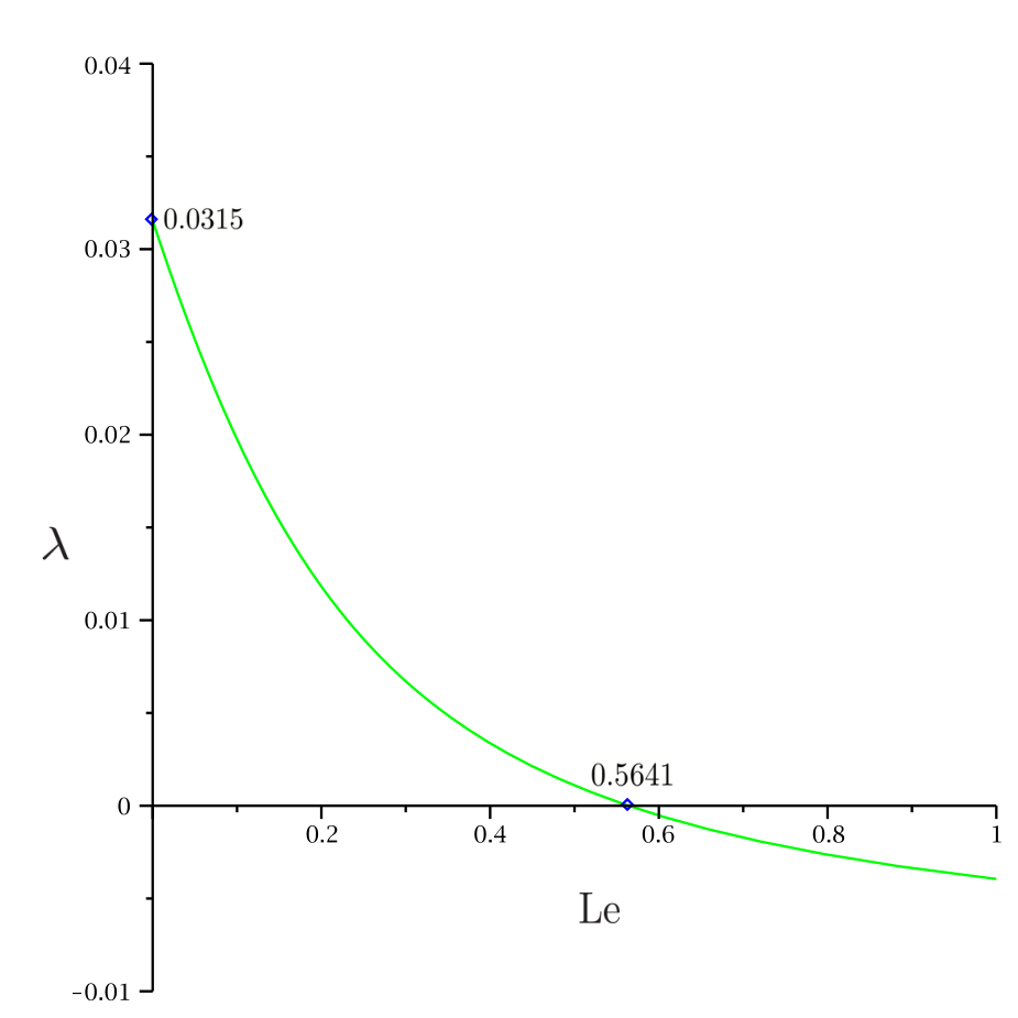
We study in a strip of ℝ2{\mathbb{R}}^{2} a combustion model of flame propagation with stepwise temperature kinetics and zero-order reaction, characterized by two free interfaces, respectively the ignition and the trailing fronts. The latter interface presents an additional difficulty because the non-degeneracy condition is not met. We turn the system to a fully nonlinear problem which is thoroughly investigated. When the width ℓ\ell of the strip is sufficiently large, we prove the existence of a critical value Lec{\rm{{Le}}}_{c} of the Lewis number Le{\rm{{Le}}}, such that the one-dimensional, planar, solution is unstable for 0<Le<Lec0<{\rm{{Le}}}<{\rm{{Le}}}_{c}. Some numerical simulations confirm the analysis.

Key words and phrases:
Free boundary problems with two free interfaces, traveling wave solutions, instability, fully nonlinear parabolic problems, analytic semigroups, dispersion relation
2000 Mathematics Subject Classification
Primary: 35R35; Secondary: 35B35, 35K50, 80A25

1. Introduction

This paper is devoted to the analysis of cellular instabilities of planar traveling fronts for a thermo-diffusive model of flame propagation with stepwise temperature kinetics and zero-order reaction. In non-dimensional form, the model reads:

{Θt=Δ​Θ+W⁡(Φ,Θ),Φt=1Le​Δ​Φ−W⁡(Φ,Θ),\displaystyle\left\{\begin{array}[]{l}\Theta_{t}=\Delta\Theta+W(\Phi,\Theta),\\[5.69054pt] \Phi_{t}=\frac{1}{{{\rm{{Le}}}}}\Delta\Phi-W(\Phi,\Theta),\end{array}\right.

where Θ\Theta and Φ\Phi are appropriately normalized temperature and concentration of deficient reactant, Le{{\rm{{Le}}}} is the Lewis number and W⁡(Φ,Θ)W(\Phi,\Theta) is a reaction rate given by

W⁡(Θ,Φ)={A,ifΘ≥ΘiandΦ>0,0,ifΘ<Θiand/orΦ=0.\displaystyle W(\Theta,\Phi)=\left\{\begin{array}[]{lllll}A,&\mbox{if}&\Theta\geq\Theta_{i}&\mbox{and}&\Phi>0,\\[5.69054pt] 0,&\mbox{if}&\Theta<\Theta_{i}&\mbox{and/or}&\Phi=0.\end{array}\right.

Here, 0<Θi<10<\Theta_{i}<1 is the ignition temperature and A>0A>0 is a normalizing factor.

Combustion models involving discontinuous reaction terms, including the system (1)-(1), have been used by physicists and engineers since the very early stage of the development of the combustion science (see Mallard and Le Châtelier [32]), primarily due to their relative simplicity and mathematical tractability (see, e.g., [4, 15, 16], and more recently [1, 3]). These models have drawn several mathematical studies on systems with discontinuous nonlinearities and related Free Boundary Problems which include, besides the pioneering work of K.-C. Chang [14], the references [12, 21, 22, 23, 24, 34, 35], to mention a few of them. In particular, models with ignition temperature were introduced in the mathematical description of the propagation of premixed flames to solve the so-called “cold-boundary difficulty” (see, e.g., [13, Section 2.2], [2]).

More specifically, in this paper we consider the free interface problem associated to the model (1)-(1). The domain is the strip ℝ×(−ℓ/2,ℓ/2)\mathbb{R}\times(-{\ell}/{2},{\ell}/{2}), the spatial coordinates are denoted by (x,y)(x,y), t>0t>0 is the time. The free interfaces are respectively the ignition interface x=F⁡(t,y)x=F(t,y) and the trailing interface x=G⁡(t,y)x=G(t,y), G⁡(t,y)<F⁡(t,y)G(t,y)<F(t,y), defined by Θ⁡(t,F⁡(t,y),y)=θi\Theta(t,F(t,y),y)=\theta_{i}, Φ⁡(t,G⁡(t,y),y)=0\Phi(t,G(t,y),y)=0. The system reads as follows, for t>0t>0 and y∈(−ℓ/2,ℓ/2)y\in(-\ell/2,\ell/2):

{∂Θ∂t​(t,x,y)=Δ​Θ​(t,x,y),x<G⁡(t,y),Φ⁡(t,x,y)=0,x<G⁡(t,y),∂Θ∂t​(t,x,y)=Δ​Θ​(t,x,y)+A,G⁡(t,y)<x<F⁡(t,y),∂Φ∂t​(t,x,y)=(Le)−1​Δ​Φ​(t,x,y)−A,G⁡(t,y)<x<F⁡(t,y),∂Θ∂t=Δ​Θ​(t,x,y),x>F⁡(t,y),∂Φ∂t=(Le)−1​Δ​Φ​(t,x,y),x>F⁡(t,y),\displaystyle\left\{\begin{array}[]{ll}\displaystyle\frac{\partial\Theta}{\partial t}(t,x,y)=\Delta\Theta(t,x,y),&x<G(t,y),\\[8.53581pt] \Phi(t,x,y)=0,&x<G(t,y),\\[5.69054pt] \displaystyle\frac{\partial\Theta}{\partial t}(t,x,y)=\Delta\Theta(t,x,y)+A,&G(t,y)<x<F(t,y),\\[8.53581pt] \displaystyle\frac{\partial\Phi}{\partial t}(t,x,y)=({\rm{{Le}}})^{-1}\Delta\Phi(t,x,y)-A,&G(t,y)<x<F(t,y),\\[8.53581pt] \displaystyle\frac{\partial\Theta}{\partial t}=\Delta\Theta(t,x,y),&x>F(t,y),\\[8.53581pt] \displaystyle\frac{\partial\Phi}{\partial t}=({\rm{{Le}}})^{-1}\Delta\Phi(t,x,y),&x>F(t,y),\end{array}\right.

where the normalizing factor AA will be fixed below. The functions Θ\Theta and Φ\Phi are continuous across the interfaces for t>0t>0, as well as their normal derivatives. As x→±∞x\to\pm\infty, it holds

(1.14) Θ⁡(t,−∞,y)=Φ⁡(t,+∞,y)=1,Θ⁡(t,+∞,y)=0.\Theta(t,-\infty,y)=\Phi(t,+\infty,y)=1,\hskip 20.00003pt\;\,\Theta(t,+\infty,y)=0.

Finally, periodic boundary conditions are assumed at y=±ℓ/2y=\pm\ell/2.

As was noted in earlier studies (see [3, 5]), this system is very different from models arising in conventional thermo-diffusive combustion. Two are the principal differences. (i) The first one is that in the model considered here, the reaction zone is of order unity, whereas in the case of Arrhenius kinetics the reaction zone is infinitely thin. This fact suggests to refer to flame fronts for stepwise temperature kinetics as thick flames, in contrast to thin flames arising in Arrhenius kinetics. (ii) The second, even more important difference, is that, in the case of Arrhenius kinetics, there is a single interface separating burned and unburned gases. In contrast to that, in case of the stepwise temperature kinetics given by (1), there are two interfaces, namely the ignition interface where Θ=Θi\Theta=\Theta_{i} located at x=F⁡(t,y)x=F(t,y), and trailing interface at x=G⁡(t,y)x=G(t,y) being defined as a largest value of xx where the concentration is equal to zero. As a consequence of (i), the normal derivatives are continuous across both interfaces, in contrast to classical models with Arrhenius kinetics where jumps occur at the flame front (see e.g., [13, Section 11.8] and [33, 37] for the related Kuramoto-Sivashinsky equation). There have been a number of mathematical works in the latter case based on the method of [8] that we are going to extend below, see in particular [6, 7, 10, 11, 28, 29, 30] for the flame front, and the references therein. Finally, note that Free Boundary Problems with two interfaces have already been considered in the literature, especially in Stefan problems, see e.g., [19, 20, 39] (one-dimensional problem) and [18] (radial solutions).

The above system admits a one-dimensional traveling wave (planar) solution (Θ(0),Φ(0))(\Theta^{(0)},\Phi^{(0)}) which propagates with constant positive velocity VV (see [3, Section 4]). It is convenient to choose the normalizing factor A=1/RA=1/R in such a way that V=1V=1, where the positive number R=R⁡(θi)R=R(\theta_{i}) is given by:

(1.15) θi​R=1−e−R,0<θi<1.\theta_{i}R=1-e^{-R},\hskip 10.00002pt0<\theta_{i}<1.

Thus, in the moving frame coordinate x′=x−tx^{\prime}=x-t, the system for the travelling wave solution reads as follows:

{Dx′​Θ(0)+Dx′​x′​Θ(0)=0,in(−∞,0],Dx′​Θ(0)+Dx′​x′​Θ(0)=−R−1,in⁡(0,R),Le​Dx′​Φ(0)+Dx′​x′​Φ(0)=Le​R−1,in⁡(0,R),Dx′​Θ(0)+Dx′​x′​Θ(0)=0,in[R,+∞),Le​Dx′​Φx′(0)+Dx′​x′​Φ(0)=0,in[R,+∞),\displaystyle\left\{\begin{array}[]{ll}D_{x^{\prime}}\Theta^{(0)}+D_{x^{\prime}x^{\prime}}\Theta^{(0)}=0,&{\rm in}\penalty\ (-\infty,0],\\[2.84526pt] D_{x^{\prime}}\Theta^{(0)}+D_{x^{\prime}x^{\prime}}\Theta^{(0)}=-R^{-1},&{\rm in}\penalty\ (0,R),\\[2.84526pt] {\rm{{Le}}}\,D_{x^{\prime}}\Phi^{(0)}+D_{x^{\prime}x^{\prime}}\Phi^{(0)}={\rm{{Le}}}R^{-1},&{\rm in}\penalty\ (0,R),\\[2.84526pt] D_{x^{\prime}}\Theta^{(0)}+D_{x^{\prime}x^{\prime}}\Theta^{(0)}=0,&{\rm in}\penalty\ [R,+\infty),\\[2.84526pt] {\rm{{Le}}}\,D_{x^{\prime}}\Phi^{(0)}_{x^{\prime}}+D_{x^{\prime}x^{\prime}}\Phi^{(0)}=0,&{\rm in}\penalty\ [R,+\infty),\end{array}\right.

whose solution is

(1.17) Θ(0)​(x′)={1,x′≤0,1+1−x′−e−x′R,x′∈(0,R),θi​eR−x′,x′≥R,Φ(0)​(x′)={0,x′≤0,e−Le​x′−1Le​R+x′R,x′∈(0,R),1+1−eLe​RLe​R​eLe​x′,x′≥R.\Theta^{(0)}(x^{\prime})=\left\{\begin{array}[]{ll}1,&x^{\prime}\leq 0,\\[5.69054pt] \displaystyle 1+\frac{1-x^{\prime}-e^{-x^{\prime}}}{R},&x^{\prime}\in(0,R),\\[5.69054pt] \displaystyle\theta_{i}e^{R-x^{\prime}},&x^{\prime}\geq R,\end{array}\right.\hskip 20.00003pt\;\,\Phi^{(0)}(x^{\prime})=\left\{\begin{array}[]{ll}0,&x^{\prime}\leq 0,\\[5.69054pt] \displaystyle\frac{e^{-{\rm{{Le}}}x^{\prime}}-1}{{\rm{{Le}}}\,R}+\frac{x^{\prime}}{R},&x^{\prime}\in(0,R),\\[5.69054pt] \displaystyle 1+\frac{1-e^{{\rm{{Le}}}R}}{{\rm{{Le}}}\,R\,e^{{\rm{{Le}}}x^{\prime}}},&x^{\prime}\geq R.\end{array}\right.
Refer to caption
Figure 1. Θ(0)\Theta^{(0)} (solid curve) and Φ(0)\Phi^{(0)} (dashed curve) with θi=0.75\theta_{i}=0.75, Le=0.75{\rm{{Le}}}=0.75 (R=0.60586R=0.60586).

The existence of traveling fronts poses a natural question of one and multidimensional stability, or especially instabilities of such fronts. It is known (see [33, 37]) that diffusional-thermal instabilities of planar flame fronts, when the Lewis number is less than unity, generates cellular flames and pattern formation. In this paper, we focus our attention on instabilities of the traveling wave (Θ(0),Φ(0))(\Theta^{(0)},\Phi^{(0)}), and thus for the ignition and the trailing interfaces. Earlier studies have shown (see [5]) that instabilities depend on the Lewis number and occur only when the width of the strip ℓ\ell is large enough (in [3], ℓ\ell is taken to infinity), which motivates the present study.

The main result of the paper is the following:

Main Theorem.

Let 0<θi<10<\theta_{i}<1 be fixed. There exist ℓ0​(θi)\ell_{0}(\theta_{i}) sufficiently large, such that, whenever ℓ>ℓ0​(θi)\ell>\ell_{0}(\theta_{i}), there exists a critical value of the Lewis number, say Lec∈(0,1){\rm{{Le}}}_{c}\in(0,1) ((see (6.2))). If Le∈(0,Lec){\rm{{Le}}}\in(0,{\rm{{Le}}}_{c}), then the traveling wave solution to problem (1)-(1.14) is unstable with respect to smooth and sufficiently small two dimensional perturbation. Further, also the ignition and the trailing interfaces are pointwise unstable.

The paper is organized as follows. In Section 2, we introduce the main notation and the functional spaces. Section 3 is devoted to transforming problem (1)-(1.14) in a fully nonlinear for problem for the perturbation of the traveling wave solution (Θ(0),Φ(0))(\Theta^{(0)},\Phi^{(0)}) in (1.17), set in a fixed domain (see (3.5)). We determine that the ignition interface meets the transversality (or non-degeneracy) condition of [8]. Unfortunately, this is not the case of the trailing interface which is of different nature. In short, the idea is to differentiate the mass fraction equation, taking advantage of the structure of the problems.

Then, in Section 4 we collect some tools that are needed to prove the main result. The theory of analytic semigroups plays a crucial role in all our analysis. For this reason, one of the main tools of this section is a generation result: we will show that a suitable realization of the linearized (at zero) elliptic operator associated with the fully nonlinear problem (3.5) generates an analytic semigroup and we characterize the interpolation spaces. This will allow us to prove an optimal regularity result for classical solutions to problem (3.5). Section 6 contains the proof of Theorem Main Theorem. Finally, Section 7 is devoted to a numerical method and computational results which show two-cell patterns (see [5] for further results).

2. Notation, functional spaces and preliminaries

In this section, we collect all the notation, the functional spaces and the preliminary results that we use throughout the paper

2.1. Notation

We find it convenient to set, for each τ>0\tau>0,

S=ℝ×(−ℓ/2,ℓ/2),Sτ+=(τ,+∞)×(−ℓ/2,ℓ/2),Sτ−=(−∞,τ)×(−ℓ/2,ℓ/2),Hτ−=(−∞,τ)×ℝ,Hτ+=(τ,+∞)×ℝ,RT=[0,T]×[−ℓ/2,ℓ/2].\displaystyle\begin{array}[]{lll}S={\mathbb{R}}\times(-\ell/2,\ell/2),&S_{\tau}^{+}=(\tau,+\infty)\times(-\ell/2,\ell/2),&S_{\tau}^{-}=(-\infty,\tau)\times(-\ell/2,\ell/2),\\[2.84526pt] H_{\tau}^{-}=(-\infty,\tau)\times{\mathbb{R}},&H_{\tau}^{+}=(\tau,+\infty)\times{\mathbb{R}},&R_{T}=[0,T]\times[-\ell/2,\ell/2].\end{array}
Functions.

Given a function f:(a,b)→ℝf:(a,b)\to{\mathbb{R}} and a point x0∈(a,b)x_{0}\in(a,b), we denote by [f]x0[f]_{x_{0}} the jump of ff at x0x_{0}, i.e., the difference f⁡(x0+)−f⁡(x0−)f(x_{0}^{+})-f(x_{0}^{-}) whenever defined. For each function f:[−ℓ/2,ℓ/2)→ℂf:[-\ell/2,\ell/2)\to{\mathbb{C}} we denote by f♯f^{\sharp} its ℓ\ell-periodic extension to ℝ{\mathbb{R}}. If ff depends also on xx running in some interval II, we still denote by f♯f^{\sharp} its periodic (with respect to yy) extension to I×ℝI\times{\mathbb{R}}. For every f∈L2((−ℓ/2,ℓ/2))f\in L^{2}((-\ell/2,\ell/2)) and k∈ℤk\in{\mathbb{Z}}, we denote by f^k\hat{f}_{k} the kk-th Fourier coefficient of ff, i.e.,

f^k=1ℓ​∫−ℓ2ℓ2f​ek¯​𝑑y,\displaystyle\hat{f}_{k}=\frac{1}{\ell}\int_{-\frac{\ell}{2}}^{\frac{\ell}{2}}f\overline{e_{k}}dy,

where eh​(y)=e2​h​π​iℓ​ye_{h}(y)=e^{\frac{2h\pi i}{\ell}y} for each h∈ℤh\in{\mathbb{Z}} and y∈ℝy\in{\mathbb{R}}. When ff depends also on the variable xx running in some interval II, f^k​(x)\hat{f}_{k}(x) stands for the kk-th Fourier coefficient of the function f⁡(x,⋅)f(x,\cdot).

The time and the spatial derivatives of a given function ff are denoted by Dt​fD_{t}f (=ft=f_{t}), Dx​fD_{x}f (=fx=f_{x}), Dy​fD_{y}f (=fy=f_{y}) Dx​x​fD_{xx}f (=fx​x=f_{xx}) Dx​y​fD_{xy}f (=fx​y=f_{xy}) and Dy​y​fD_{yy}f (=fy​y=f_{yy}), respectively. If β=(β1,β2)\beta=(\beta_{1},\beta_{2}) with β1,β2∈ℕ∪{0}\beta_{1},\beta_{2}\in{\mathbb{N}}\cup\{0\}, then we set Dγ=Dxγ1​Dyγ2D^{\gamma}=D^{\gamma_{1}}_{x}D^{\gamma_{2}}_{y}.

Finally, we denote by χA\chi_{A} the characteristic function of the set A⊂ℝdA\subset\mathbb{R}^{d} (d≥1d\geq 1).

Miscellanea

Throughout the paper, we denote by cλc_{\lambda} a positive constant, possibly depending on λ\lambda but being independent of kk, nn, xx and the functions that we will consider, which may vary from line to line. We simply write cc when the constant is independent also of λ\lambda.

The subscript “bb” stands for bounded. For instance Cb​(Ω,ℂ)C_{b}(\Omega;{\mathbb{C}}) denotes the set of bounded and continuous function from Ω\Omega to ℂ{\mathbb{C}}. When we deal with spaces of real-valued functions we omit to write “ℂ{\mathbb{C}}”.

Vector-valued functions are displayed in bold.

2.2. Main function spaces

Here, we collect the main function spaces used in the paper pointing out the (sub)section where they are used for the first time.

The spaces 𝒳\bm{\mathcal{X}} and 𝒳k+α\bm{\mathcal{X}}_{k+\alpha} (Section 4)

By 𝓧\bm{\mathcal{X}} we denote the set of all pairs 𝐟=(f1,f2){\bf f}=(f_{1},f_{2}), where f1:S¯→ℂf_{1}:\overline{S}\to{\mathbb{C}} and f2:S0+¯→ℂf_{2}:\overline{S_{0}^{+}}\to{\mathbb{C}} are bounded functions, f1∈C(S0−¯;ℂ)∩C([0,R]×[−ℓ/2,ℓ/2];ℂ)∩C(SR+¯;ℂ)f_{1}\in C(\overline{S_{0}^{-}};{\mathbb{C}})\cap C([0,R]\times[-\ell/2,\ell/2];{\mathbb{C}})\cap C(\overline{S_{R}^{+}};{\mathbb{C}}), f2∈C([0,R]×[−ℓ/2,ℓ/2];ℂ)∩C(SR+¯;ℂ)f_{2}\in C([0,R]\times[-\ell/2,\ell/2];{\mathbb{C}})\cap C(\overline{S_{R}^{+}};{\mathbb{C}}) and limx→±∞f1​(x,y)=limx→+∞f2​(x,y)=0\lim_{x\to\pm\infty}f_{1}(x,y)=\lim_{x\to+\infty}f_{2}(x,y)=0 for each y∈[−ℓ/2,ℓ/2]y\in[-\ell/2,\ell/2]. It is endowed with the sup-norm, i.e., ‖𝐟‖∞=‖f1‖L∞​(S,ℂ)+‖f2‖L∞​(S0+,ℂ)\|{\bf f}\|_{\infty}=\|f_{1}\|_{L^{\infty}(S;{\mathbb{C}})}+\|f_{2}\|_{L^{\infty}(S_{0}^{+};{\mathbb{C}})}.

For each α∈(0,1]\alpha\in(0,1], 𝓧α\bm{\mathcal{X}}_{\alpha} denotes the subset of 𝓧\bm{\mathcal{X}} of all 𝐟{\bf f} such that (i) f1∈Cbα(S0−¯;ℂ)∩Cbα([0,R]×[−ℓ/2,ℓ/2];ℂ)∩Cbα(SR+¯;ℂ)f_{1}\in C^{\alpha}_{b}(\overline{S_{0}^{-}};{\mathbb{C}})\cap C^{\alpha}_{b}([0,R]\times[-\ell/2,\ell/2];{\mathbb{C}})\cap C^{\alpha}_{b}(\overline{S_{R}^{+}};{\mathbb{C}}), (ii) f2∈Cbα([0,R]×[−ℓ/2,ℓ/2];ℂ)∩Cbα(SR+¯;ℂ)f_{2}\in C^{\alpha}_{b}([0,R]\times[-\ell/2,\ell/2];{\mathbb{C}})\cap C^{\alpha}_{b}(\overline{S_{R}^{+}};{\mathbb{C}}), (iii) fj(⋅,−ℓ/2)=fj(⋅,ℓ/2)f_{j}(\cdot,-\ell/2)=f_{j}(\cdot,\ell/2) (and ∇fj(⋅,−ℓ/2)=∇fj(⋅,ℓ/2)\nabla f_{j}(\cdot,-\ell/2)=\nabla f_{j}(\cdot,\ell/2) if α=1\alpha=1) for j=1,2j=1,2. It is endowed with the norm ∥𝐟∥α=∥f1∥Cbα​(S0−¯,ℂ)+∑j=12(∥fj∥Cαb([0,R]×[−ℓ/2,ℓ/2];ℂ)+∥fj∥Cbα​(SR+¯,ℂ))\|{\bf f}\|_{\alpha}=\|f_{1}\|_{C^{\alpha}_{b}(\overline{S_{0}^{-}};{\mathbb{C}})}+\sum_{j=1}^{2}(\|f_{j}\|_{C^{\alpha}_{b}([0,R]\times[-\ell/2,\ell/2];{\mathbb{C}})}+\|f_{j}\|_{C^{\alpha}_{b}(\overline{S_{R}^{+}};{\mathbb{C}})}).

For k∈ℕk\in{\mathbb{N}} and α∈(0,1)\alpha\in(0,1), 𝓧k+α\bm{\mathcal{X}}_{k+\alpha} (k∈ℕk\in{\mathbb{N}}, α∈(0,1)\alpha\in(0,1)) denotes the set of all 𝐟∈𝓧{\bf f}\in\bm{\mathcal{X}} such that Dβ​𝐟=(Dγ​f1,Dγ​f2)∈𝓧D^{\beta}{\bf f}=(D^{\gamma}f_{1},D^{\gamma}f_{2})\in\bm{\mathcal{X}}, Dγfj(⋅,−ℓ/2)=Dγfj(⋅,ℓ/2)D^{\gamma}f_{j}(\cdot,-\ell/2)=D^{\gamma}f_{j}(\cdot,\ell/2) for each |γ|≤k|\gamma|\leq k, j=1,2j=1,2, and Dγ​𝐟∈𝓧αD^{\gamma}{\bf f}\in\bm{\mathcal{X}}_{\alpha} for |γ|=k|\gamma|=k. It is endowed with the norm ‖𝐟‖k+α:=∑|γ|<k‖Dγ​𝐟‖∞+∑|γ|=k‖Dγ​𝐟‖α\|{\bf f}\|_{k+\alpha}:=\sum_{|\gamma|<k}\|{D^{\gamma}{\bf f}}\|_{\infty}+\sum_{|\gamma|=k}\|D^{\gamma}{\bf f}\|_{\alpha}.

The spaces 𝒴α​(a,b)\bm{\mathcal{Y}}_{\alpha}(a,b) and 𝒴2+α​(a,b)\bm{\mathcal{Y}}_{2+\alpha}(a,b) (Section 5)

For α∈(0,1)\alpha\in(0,1) and 0≤a<b0\leq a<b, we define by 𝓨α​(a,b)\bm{\mathcal{Y}}_{\alpha}(a,b) the space of all pairs 𝐟=(f1,f2){\bf f}=(f_{1},f_{2}) such that f1:[a,b]×S¯→ℝf_{1}:[a,b]\times\overline{S}\to{\mathbb{R}}, f2:[a,b]×S0+¯→ℝf_{2}:[a,b]\times\overline{S_{0}^{+}}\to{\mathbb{R}} and

‖𝐟‖𝓨α​(a,b)=supa<t<b‖𝐟⁡(t,⋅,⋅)‖α+sup(x,y)∈S‖f1​(⋅,x,y)‖Cα/2​((,,,))+sup(x,y)∈S0+‖f2​(⋅,x,y)‖Cα/2​((,,,))<+∞.\displaystyle\|{\bf f}\|_{\bm{\mathcal{Y}}_{\alpha}(a,b)}=\sup_{a<t<b}\|{\bf f}(t,\cdot,\cdot)\|_{\alpha}+\sup_{(x,y)\in S}\|f_{1}(\cdot,x,y)\|_{C^{\alpha/2}((a,b))}+\sup_{(x,y)\in S^{+}_{0}}\|f_{2}(\cdot,x,y)\|_{C^{\alpha/2}((a,b))}<+\infty.

Similarly, 𝓨2+α​(a,b)\bm{\mathcal{Y}}_{2+\alpha}(a,b) denotes the space of all the pairs 𝐮{\bf u} such that Dtγ1​Dxγ2​Dyγ3​𝐮D^{\gamma_{1}}_{t}D^{\gamma_{2}}_{x}D^{\gamma_{3}}_{y}{\bf u} belongs to 𝓨α​(a,b)\bm{\mathcal{Y}}_{\alpha}(a,b) for every γ1,γ2,γ3≥0\gamma_{1},\gamma_{2},\gamma_{3}\geq 0 such that 2​γ1+γ2+γ3≤22\gamma_{1}+\gamma_{2}+\gamma_{3}\leq 2. These are Banach spaces with the norms ∥⋅∥𝓨α​(a,b)\|\cdot\|_{\bm{\mathcal{Y}}_{\alpha}(a,b)} and ‖𝐮‖𝓨2+α​(a,b)=∑2​γ1+γ2+γ3≤2‖Dtγ1​Dxγ2​Dyγ3​𝐮‖𝓨α​(a,b)\|{\bf u}\|_{\bm{\mathcal{Y}}_{2+\alpha}(a,b)}=\sum_{2\gamma_{1}+\gamma_{2}+\gamma_{3}\leq 2}\|D^{\gamma_{1}}_{t}D^{\gamma_{2}}_{x}D^{\gamma_{3}}_{y}{\bf u}\|_{\bm{\mathcal{Y}}_{\alpha}(a,b)}.

If a=0a=0 and b=Tb=T then we simply write 𝓨α\bm{\mathcal{Y}}_{\alpha} and 𝓨2+α\bm{\mathcal{Y}}_{2+\alpha} instead of 𝓨α​(0,T)\bm{\mathcal{Y}}_{\alpha}(0,T) and 𝓨2+α​(0,T)\bm{\mathcal{Y}}_{2+\alpha}(0,T), respectively.

3. Derivation of the fully nonlinear problem

3.1. The system on a fixed domain

To begin with, we rewrite System (1) in the coordinates t′=tt^{\prime}=t, x′=x−tx^{\prime}=x-t, y′=yy^{\prime}=y, Dt=Dt′−Dx′D_{t}=D_{t^{\prime}}-D_{x^{\prime}}. Next, we look for the free interfaces respectively as:

G⁡(t′,y′)=g⁡(t′,y′),F⁡(t′,y′)=R+f⁡(t′,y′),G(t^{\prime},y^{\prime})=g(t^{\prime},y^{\prime}),\hskip 20.00003pt\;\,F(t^{\prime},y^{\prime})=R+f(t^{\prime},y^{\prime}),

where ff and gg are small perturbations. In other words, the space variable x′x^{\prime} varies from −∞-\infty to g⁡(t′,y′)g(t^{\prime},y^{\prime}), from g⁡(t′,y′)g(t^{\prime},y^{\prime}) to R+f⁡(t′,y′)R+f(t^{\prime},y^{\prime}), and eventually from R+f⁡(t′,y′)R+f(t^{\prime},y^{\prime}) to +∞+\infty. As usual, it is convenient to transform the problem on a variable domain to a problem on a fixed domain. To this end, we define a coordinate transformation in the spirit of [8, Section 2.1]:

t′=τ,x′=ξ+β⁡(ξ)​g​(τ,η)+β⁡(ξ−R)​f​(τ,η),y′=η,t^{\prime}=\tau,\hskip 20.00003pt\;\,x^{\prime}=\xi+\beta(\xi)g(\tau,\eta)+\beta(\xi-R)f(\tau,\eta),\hskip 20.00003pt\;\,y^{\prime}=\eta,

where β\beta is a smooth mollifier, equal to unity in a small neighborhood of ξ=0\xi=0, say [−δ,δ][-\delta,\delta], and has compact support contained in (−2​δ,2​δ)⊂(−R,R)(-2\delta,2\delta)\subset(-R,R). When x′=gx^{\prime}=g, ξ=0\xi=0, and ξ=R\xi=R when x′=R+fx^{\prime}=R+f. Then, the trailing front and the ignition front are fixed at ξ=0\xi=0 and ξ=R\xi=R, respectively. Thanks to the translation invariance, (1.17) holds with the variable ξ\xi. For convenience, we introduce the notation

(3.1) ϱ⁡(τ,ξ,η)=β⁡(ξ)​g​(τ,η)+β⁡(ξ−R)​f​(τ,η)\varrho(\tau,\xi,\eta)=\beta(\xi)g(\tau,\eta)+\beta(\xi-R)f(\tau,\eta)

and we expand (1+ϱξ)−1=1−ϱξ+(ϱξ)2​(1+ϱξ)−1(1+\varrho_{\xi})^{-1}=1-\varrho_{\xi}+(\varrho_{\xi})^{2}(1+\varrho_{\xi})^{-1}. It turns out that

Dx′=Dξ−ϱξ​Dξ+(ϱξ)2​(1+ϱξ)−1​Dξ,\displaystyle D_{x^{\prime}}=D_{\xi}-\varrho_{\xi}D_{\xi}+(\varrho_{\xi})^{2}(1+\varrho_{\xi})^{-1}D_{\xi},
Dt′=Dτ−ϱτ​Dξ+ϱτ​ϱξ​Dξ−ϱτ​(ϱξ)2​(1+ϱξ)−1​Dξ,\displaystyle D_{t^{\prime}}=D_{\tau}-\varrho_{\tau}D_{\xi}+\varrho_{\tau}\varrho_{\xi}D_{\xi}-\varrho_{\tau}(\varrho_{\xi})^{2}(1+\varrho_{\xi})^{-1}D_{\xi},
Dy′=Dη−ϱη​Dξ+ϱη​ϱξ​Dξ−ϱη​(ϱξ)2​(1+ϱξ)−1​Dξ\displaystyle D_{y^{\prime}}=D_{\eta}-\varrho_{\eta}D_{\xi}+\varrho_{\eta}\varrho_{\xi}D_{\xi}-\varrho_{\eta}(\varrho_{\xi})^{2}(1+\varrho_{\xi})^{-1}D_{\xi}

and System (1) reads:

(3.2) Θτ=Θξ+Δ​Θ+(ϱη2−ϱξ2−2​ϱξ)​(1+ϱξ)−2​Θξ​ξ−2​ϱη​(1+ϱξ)−1​Θξ​η+[(ϱτ−ϱξ−ϱη​η)​(1+ϱξ)−1+2​ϱη​ϱξ​η​(1+ϱξ)−2−ϱξ​ξ​(1+ϱη2)​(1+ϱξ)−3]​Θξ,Φ=0\displaystyle\begin{split}\Theta_{\tau}=&\Theta_{\xi}+\Delta\Theta+(\varrho_{\eta}^{2}-\varrho_{\xi}^{2}-2\varrho_{\xi})(1+\varrho_{\xi})^{-2}\Theta_{\xi\xi}-2\varrho_{\eta}(1+\varrho_{\xi})^{-1}\Theta_{\xi\eta}\\ &+\big[(\varrho_{\tau}-\varrho_{\xi}-\varrho_{\eta\eta})(1+\varrho_{\xi})^{-1}+2\varrho_{\eta}\varrho_{\xi\eta}(1+\varrho_{\xi})^{-2}-\varrho_{\xi\xi}(1+\varrho_{\eta}^{2})(1+\varrho_{\xi})^{-3}\big]\Theta_{\xi},\\[5.69054pt] \Phi=&0\end{split}

in (0,+∞)×(−∞,0)×(−ℓ/2,ℓ/2)(0,+\infty)\times(-\infty,0)\times(-\ell/2,\ell/2),

(3.3) Θτ=Θξ+Δ​Θ+(ϱη2−ϱξ2−2​ϱξ)​(1+ϱξ)−2​Θξ​ξ−2​ϱη​(1+ϱξ)−1​Θξ​η+R−1+[(ϱτ−ϱξ−ϱη​η)​(1+ϱξ)−1+2​ϱη​ϱξ​η​(1+ϱξ)−2−ϱξ​ξ​(1+ϱη2)​(1+ϱξ)−3]​Θξ,Φτ=Φξ+Le−1​Δ​Φ+Le−1​(ϱη2−ϱξ2−2​ϱξ)​(1+ϱξ)−2​Φξ​ξ−2​L​e−1​ϱη​(1+ϱξ)−1​Φξ​η−R−1+[(ϱτ−ϱξ−Le−1​ϱη​η)​(1+ϱξ)−1+2​L​e−1​ϱη​ϱξ​η​(1+ϱξ)−2−Le−1​ϱξ​ξ​(1+ϱη2)​(1+ϱξ)−3]​Φξ\displaystyle\begin{split}\Theta_{\tau}=&\Theta_{\xi}+\Delta\Theta+(\varrho_{\eta}^{2}-\varrho_{\xi}^{2}-2\varrho_{\xi})(1+\varrho_{\xi})^{-2}\Theta_{\xi\xi}-2\varrho_{\eta}(1+\varrho_{\xi})^{-1}\Theta_{\xi\eta}+R^{-1}\\ &+\big[(\varrho_{\tau}-\varrho_{\xi}-\varrho_{\eta\eta})(1+\varrho_{\xi})^{-1}+2\varrho_{\eta}\varrho_{\xi\eta}(1+\varrho_{\xi})^{-2}-\varrho_{\xi\xi}(1+\varrho_{\eta}^{2})(1+\varrho_{\xi})^{-3}\big]\Theta_{\xi},\\[5.69054pt] \Phi_{\tau}=&\Phi_{\xi}+{\rm{{Le}}}^{-1}\Delta\Phi+{\rm{{Le}}}^{-1}(\varrho_{\eta}^{2}-\varrho_{\xi}^{2}-2\varrho_{\xi})(1+\varrho_{\xi})^{-2}\Phi_{\xi\xi}-2{\rm{{Le}}}^{-1}\varrho_{\eta}(1+\varrho_{\xi})^{-1}\Phi_{\xi\eta}-R^{-1}\\ &+[(\varrho_{\tau}\!-\!\varrho_{\xi}\!-\!{\rm{{Le}}}^{-1}\varrho_{\eta\eta})(1+\varrho_{\xi})^{-1}\!+\!2{\rm{{Le}}}^{-1}\varrho_{\eta}\varrho_{\xi\eta}(1+\varrho_{\xi})^{-2}-{\rm{{Le}}}^{-1}\varrho_{\xi\xi}(1+\varrho_{\eta}^{2})(1+\varrho_{\xi})^{-3}]\Phi_{\xi}\end{split}

in (0,+∞)×(0,R)×(−ℓ/2,ℓ/2)(0,+\infty)\times(0,R)\times(-\ell/2,\ell/2) and

(3.4) Θτ=Θξ+Δ​Θ+(ϱη2−ϱξ2−2​ϱξ)​(1+ϱξ)−2​Θξ​ξ−2​ϱη​(1+ϱξ)−1​Θξ​η+[(ϱτ−ϱξ−ϱη​η)​(1+ϱξ)−1+2​ϱη​ϱξ​η​(1+ϱξ)−2−ϱξ​ξ​(1+ϱη2)​(1+ϱξ)−3]​Θξ,Φτ=Φξ+Le−1​Δ​Φ+Le−1​(ϱη2−ϱξ2−2​ϱξ)​(1+ϱξ)−2​Φξ​ξ−2​L​e−1​ϱη​(1+ϱξ)−1​Φξ​η+[(ϱτ−ϱξ−Le−1​ϱη​η)​(1+ϱξ)−1+2​L​e−1​ϱη​ϱξ​η​(1+ϱξ)−2−Le−1​ϱξ​ξ​(1+ϱη2)​(1+ϱξ)−3]​Φξ\displaystyle\begin{split}\Theta_{\tau}=&\Theta_{\xi}+\Delta\Theta+(\varrho_{\eta}^{2}-\varrho_{\xi}^{2}-2\varrho_{\xi})(1+\varrho_{\xi})^{-2}\Theta_{\xi\xi}-2\varrho_{\eta}(1+\varrho_{\xi})^{-1}\Theta_{\xi\eta}\\ &+\big[(\varrho_{\tau}-\varrho_{\xi}-\varrho_{\eta\eta})(1+\varrho_{\xi})^{-1}+2\varrho_{\eta}\varrho_{\xi\eta}(1+\varrho_{\xi})^{-2}-\varrho_{\xi\xi}(1+\varrho_{\eta}^{2})(1+\varrho_{\xi})^{-3}\big]\Theta_{\xi},\\[5.69054pt] \Phi_{\tau}=&\Phi_{\xi}+{\rm{{Le}}}^{-1}\Delta\Phi+{\rm{{Le}}}^{-1}(\varrho_{\eta}^{2}-\varrho_{\xi}^{2}-2\varrho_{\xi})(1+\varrho_{\xi})^{-2}\Phi_{\xi\xi}-2{\rm{{Le}}}^{-1}\varrho_{\eta}(1+\varrho_{\xi})^{-1}\Phi_{\xi\eta}\\ &+\big[(\varrho_{\tau}\!-\!\varrho_{\xi}\!-\!{\rm{{Le}}}^{-1}\varrho_{\eta\eta})(1+\varrho_{\xi})^{-1}\!+\!2{\rm{{Le}}}^{-1}\varrho_{\eta}\varrho_{\xi\eta}(1+\varrho_{\xi})^{-2}-{\rm{{Le}}}^{-1}\varrho_{\xi\xi}(1+\varrho_{\eta}^{2})(1+\varrho_{\xi})^{-3}\big]\Phi_{\xi}\end{split}

in (0,+∞)×(R,+∞)×(−ℓ/2,ℓ/2)(0,+\infty)\times(R,+\infty)\times(-\ell/2,\ell/2). Moreover, Θ\Theta and Φ\Phi are continuous at the (fixed) interfaces ξ=0\xi=0 and ξ=R\xi=R, and so are their first-order derivatives. Thus,

[Θ⁡(τ,⋅,η)]0=[Θξ​(τ,⋅,η)]0=Φ⁡(τ,0,η)=Φξ​(τ,0,η)=0[\Theta(\tau,\cdot,\eta)]_{0}=[\Theta_{\xi}(\tau,\cdot,\eta)]_{0}=\Phi(\tau,0,\eta)=\Phi_{\xi}(\tau,0,\eta)=0

and

Θ⁡(τ,R,η)=θi,[Θ⁡(τ,⋅,η)]R=[Θξ​(τ,⋅,η)]R=[Φ⁡(τ,⋅,η)]=[Φξ​(τ,⋅,η)]=0.\Theta(\tau,R,\eta)=\theta_{i},\hskip 10.00002pt[\Theta(\tau,\cdot,\eta)]_{R}=[\Theta_{\xi}(\tau,\cdot,\eta)]_{R}=[\Phi(\tau,\cdot,\eta)]=[\Phi_{\xi}(\tau,\cdot,\eta)]=0.

Conditions (1.14) hold at ξ=±∞\xi=\pm\infty and periodic boundary conditions are assumed at η=±ℓ/2\eta=\pm\ell/2.

3.2. Elimination of the interfaces

From now on, with a slight abuse of notation, which does not cause confusion, we write tt instead of τ\tau and xx, yy instead of ξ\xi and η\eta.

In the spirit of [8, 29], we introduce the splitting:

(3.5) Θ⁡(t,x,y)=Θ(0)​(x)+ϱ⁡(t,x,y)​Θx(0)​(x)+u⁡(t,x,y),\displaystyle\Theta(t,x,y)=\Theta^{(0)}(x)+\varrho(t,x,y)\Theta^{(0)}_{x}(x)+u(t,x,y),
(3.6) Φ⁡(t,x,y)=Φ(0)​(x)+ϱ⁡(t,x,y)​Φx(0)​(x)+v⁡(t,x,y),\displaystyle\Phi(t,x,y)=\Phi^{(0)}(x)+\varrho(t,x,y)\Phi^{(0)}_{x}(x)+v(t,x,y),

which is a sort of Taylor expansion of (Θ,Φ)(\Theta,\Phi) around the travelling wave solution (Θ(0),Φ(0))(\Theta^{(0)},\Phi^{(0)}). Thus, the pair (u,v)(u,v) plays the role of a remainder and, since we are interested in stability issues, we can assume that uu and vv are “sufficiently small” in a sense which will be made precise later on.

A long but straightforward computation reveals that the pair (u,v)(u,v) satisfies the differential equations

(3.7) ut=ux+Δ​u+ϱt​(1+ϱx)−1​(ϱ​Θx​x(0)+ux)−(1+ϱx)−3​ϱx​x​(1+ϱy2)​(ϱ​Θx​x(0)+ux)−(1+ϱx)−1​[(ϱx+ϱy​y)​(ϱ​Θx​x(0)+ux)+2​ϱy​(ϱy​Θx​x(0)+ux​y)]+(1+ϱx)−2[2ϱyϱx​y(ϱΘ(0)x​x+ux)+(ϱy2−ϱx2)(ϱΘ(0)x​x​x+Θ(0)x​x+ux​x)−2ϱx(ϱΘ(0)x​x​x−ϱy2Θ(0)x​x+ux​x)],\displaystyle\begin{split}u_{t}=&u_{x}+\Delta u+\varrho_{t}(1+\varrho_{x})^{-1}(\varrho\Theta^{(0)}_{xx}+u_{x})-(1+\varrho_{x})^{-3}\varrho_{xx}(1+\varrho_{y}^{2})(\varrho\Theta^{(0)}_{xx}+u_{x})\\ &-(1+\varrho_{x})^{-1}\big[(\varrho_{x}+\varrho_{yy})(\varrho\Theta^{(0)}_{xx}+u_{x})+2\varrho_{y}(\varrho_{y}\Theta^{(0)}_{xx}+u_{xy})\big]\\ &+(1+\varrho_{x})^{-2}\big[2\varrho_{y}\varrho_{xy}(\varrho\Theta^{(0)}_{xx}+u_{x})+(\varrho_{y}^{2}-\varrho_{x}^{2})(\varrho\Theta^{(0)}_{xxx}+\Theta^{(0)}_{xx}+u_{xx})\\ &\phantom{+(1+\varrho_{x})^{-2}\big[\;\,}-2\varrho_{x}(\varrho\Theta^{(0)}_{xxx}-\varrho_{y}^{2}\Theta^{(0)}_{xx}+u_{xx})\big],\end{split}

in (0,+∞)×(ℝ∖{0,R})×(−ℓ/2,ℓ/2)(0,+\infty)\times({\mathbb{R}}\setminus\{0,R\})\times(-\ell/2,\ell/2) and

(3.8) vt=vx+Le−1​Δ​v+ϱt​(1+ϱx)−1​(ϱ​Φx​x(0)+vx)−Le−1​(1+ϱx)−3​ϱx​x​(1+ϱy2)​(ϱ​Φx​x(0)+vx)−Le−1​(1+ϱx)−1​[(Le​ϱx+ϱy​y)​(ϱ​Φx​x(0)+vx)+2​ϱy​(ϱy​Φx​x(0)+vx​y)]+Le−1(1+ϱx)−2[2ϱyϱx​y(ϱΦ(0)x​x+vx)+(ϱy2−ϱx2)(ϱΦ(0)x​x​x+Φ(0)x​x+vx​x)−2ϱx(ϱΦ(0)x​x​x−ϱy2Φ(0)x​x+vx​x)]\displaystyle\begin{split}v_{t}=&v_{x}+{\rm{{Le}}}^{-1}\Delta v+\varrho_{t}(1+\varrho_{x})^{-1}(\varrho\Phi^{(0)}_{xx}+v_{x})-{\rm{{Le}}}^{-1}(1+\varrho_{x})^{-3}\varrho_{xx}(1+\varrho_{y}^{2})(\varrho\Phi^{(0)}_{xx}+v_{x})\\ &-{\rm{{Le}}}^{-1}(1+\varrho_{x})^{-1}\big[({\rm{{Le}}}\,\varrho_{x}+\varrho_{yy})(\varrho\Phi^{(0)}_{xx}+v_{x})+2\varrho_{y}(\varrho_{y}\Phi^{(0)}_{xx}+v_{xy})\big]\\ &+{\rm{{Le}}}^{-1}(1+\varrho_{x})^{-2}\big[2\varrho_{y}\varrho_{xy}(\varrho\Phi^{(0)}_{xx}+v_{x})+(\varrho_{y}^{2}-\varrho_{x}^{2})(\varrho\Phi^{(0)}_{xxx}+\Phi^{(0)}_{xx}+v_{xx})\\ &\phantom{+{\rm{{Le}}}^{-1}(1+\varrho_{x})^{-2}\big[\;\,}-2\varrho_{x}(\varrho\Phi^{(0)}_{xxx}-\varrho_{y}^{2}\Phi^{(0)}_{xx}+v_{xx})\big]\end{split}

in (0,+∞)×[(0,R)∪(R,+∞)]×(−ℓ/2,ℓ/2)(0,+\infty)\times[(0,R)\cup(R,+\infty)]\times(-\ell/2,\ell/2) and v=0v=0 in (0,+∞)×(−∞,0)×(−ℓ/2,ℓ/2)(0,+\infty)\times(-\infty,0)\times(-\ell/2,\ell/2).

Two steps are still needed:

(a) we have to determine the jump conditions satisfied by uu and vv;

(b) again in the spirit of [8, 29], we have to get rid of the function φ\varphi from the right-hand sides of (3.7) and (3.8). As we will see, some difficulties appear and, to overcome them, we will differentiate the differential equation (3.8).

3.2.1. The ignition interface x=R\bm{x=R}.

Note that Θ(0)\Theta^{(0)}, Φ(0)\Phi^{(0)} belong to C1​(ℝ)C^{1}({\mathbb{R}}). Thus, [u]R=[v]R=0[u]_{R}=[v]_{R}=0. Moreover, Θx(0)​(R)=−θi\Theta^{(0)}_{x}(R)=-\theta_{i} and Φx(0)​(R)=(1−exp⁡(−Le​R))/R\Phi^{(0)}_{x}(R)=(1-\exp(-{\rm{{Le}}}R))/R, so that they do not vanish at the interface x=Rx=R. The latter is a kind of transversality or non-degeneracy condition (see [8]). Evaluating (3.5) at x=Rx=R, we get u⁡(R)=θi​fu(R)=\theta_{i}f.

Next, differentiating (3.5) and (3.6) for x≠Rx\neq R, and taking the jumps across x=Rx=R, it is not difficult to show that [ux]R=−R−1​f[u_{x}]_{R}=-R^{-1}f and [vx]R=R−1​Le​f[v_{x}]_{R}=R^{-1}{\rm{{Le}}}\,f. This is a key point since we are able to express ff in terms of uu and write

(3.9) f⁡(t,y)=θi−1​u​(t,R,y).f(t,y)={\theta_{i}}^{-1}u(t,R,y).

Summing up, the interface conditions at x=Rx=R are the following:

(3.10) [u]R=[v]R=0,u⁡(R)+θi​R​[ux]R=0,Le​[ux]R+[vx]R=0.[u]_{R}=[v]_{R}=0,\hskip 10.00002ptu(R)+\theta_{i}R[u_{x}]_{R}=0,\hskip 20.00003pt\;\,{\rm{{Le}}}[u_{x}]_{R}+[v_{x}]_{R}=0.

3.2.2. The trailing interface x=𝟎\bm{x=0}.

Taking the jump at x=0x=0 of both sides of (3.5) and (3.6), we get the conditions [u]0=v⁡(0)=0[u]_{0}=v(0)=0 for uu and vv. The trailing interface has a different nature with respect to the ignition interface. Indeed, since Θx(0)​(0)=Φx(0)​(0)=0\Theta^{(0)}_{x}(0)=\Phi^{(0)}_{x}(0)=0, the non-degeneracy condition of [8] is not verified and we are able to express gg in terms neither of uu or vv. On the other hand, Θx​x(0)​(0+)=−R−1\Theta^{(0)}_{xx}(0^{+})=-R^{-1} and Φx​x(0)​(0+)=R−1​Le\Phi^{(0)}_{xx}(0^{+})=R^{-1}{\rm{{Le}}}, so that they do not vanish. Differentiating (3.5) and (3.6) for x≠0x\neq 0, and taking the jumps yields: [ux]0=R−1​g[u_{x}]_{0}=R^{-1}g, vx​(⋅,0+,⋅)=−R−1​g​Lev_{x}(\cdot,0^{+},\cdot)=-R^{-1}g{\rm{{Le}}}. Hence, we get the additional interface condition Le​[ux]0+vx​(⋅,0+,⋅)=0{\rm{{Le}}}\,[u_{x}]_{0}+v_{x}(\cdot,0^{+},\cdot)=0, so that the interface conditions at x=0x=0 are

(3.11) [u]0=v⁡(0)=0,Le​[ux]0+vx​(⋅,0+,⋅)=0.[u]_{0}=v(0)=0,\hskip 10.00002pt{\rm{{Le}}}\,[u_{x}]_{0}+v_{x}(\cdot,0^{+},\cdot)=0.

We can also write

(3.12) g⁡(t,y)=−R​Le−1​vx​(t,0+,y).g(t,y)=-R\,{{\rm{{Le}}}}^{-1}v_{x}(t,0^{+},y).

Although the front gg could be eliminated, the method of [8] is not applicable since, in contrast to (3.9), gg is related to the derivative of vv in the equation (3.12).

3.3. Differentiation and new interface conditions

To overcome the difficulty pointed out above, the trick is to differentiate (3.8) with respect to xx, taking advantage of the structure of the system and consider the problem satisfied by the pair (u,vx)(u,v_{x}). From (3.10) and (3.11) we get the following interface conditions for uu and w=vxw=v_{x}:

(3.13) [u]0=0,Le[ux]0+w(0+)=0,[u]R=0,u(R)+θiR[ux]R=0,Le[ux]R+[w]R=0.\displaystyle\begin{split}&[u]_{0}=0,\qquad\;\,{\rm{{Le}}}\,[u_{x}]_{0}+w(0^{+})=0,\\ &[u]_{R}=0,\qquad\;\,u(R)+\theta_{i}R[u_{x}]_{R}=0,\qquad\;\,{\rm{{Le}}}[u_{x}]_{R}+[w]_{R}=0.\end{split}

We missed two jump conditions: one at the trailing interface and the other one at the ignition interface. To obtain the additional condition at the trailing interface x=0x=0, we differentiate (3.6) twice in a neighborhood of x=0x=0 and take the trace at x=0+x=0^{+}. Using (3.12), we get

(3.14) Φx​x​(⋅,0+,⋅)=Le​R−1+Le​w​(⋅,0+,⋅)+wx​(⋅,0+,⋅).\Phi_{xx}(\cdot,0^{+},\cdot)={\rm{{Le}}}\,R^{-1}+{\rm{{Le}}}\,w(\cdot,0^{+},\cdot)+w_{x}(\cdot,0^{+},\cdot).

To get rid of Φx​x​(⋅,0+,⋅)\Phi_{xx}(\cdot,0^{+},\cdot) from the left-hand side of (3.14), we observe that, for x>0x>0 sufficiently small, the second equation in (3.3) reduces to

(3.15) Φt=Φx+Le−1​Δ​Φ+Le−1​gy2​Φx​x−2​L​e−1​gy​Φx​y−R−1+(gt−Le−1​gy​y)​Φx.\displaystyle\begin{split}\Phi_{t}=&\Phi_{x}+{\rm{{Le}}}^{-1}\Delta\Phi+{\rm{{Le}}}^{-1}g_{y}^{2}\Phi_{xx}-2{\rm{{Le}}}^{-1}g_{y}\Phi_{xy}-R^{-1}+(g_{t}-{\rm{{Le}}}^{-1}g_{yy})\Phi_{x}.\end{split}

Taking the trace of (3.15) at x=0+x=0^{+} it is easy to check that Φx​x​(⋅,0+,⋅)​(1+gy2)=Le​R−1\Phi_{xx}(\cdot,0^{+},\cdot)(1+g_{y}^{2})={\rm{{Le}}}\,R^{-1}. Hence, using (3.12) and (3.14) we get the additional interface condition

(3.16) Le​w​(⋅,0+,⋅)+wx​(⋅,0+,⋅)=Le​R−1​{[1+R2​Le−2​(wy​(⋅,0+,⋅))2]−1−1}.{\rm{{Le}}}\,w(\cdot,0^{+},\cdot)+w_{x}(\cdot,0^{+},\cdot)={\rm{{Le}}}\,R^{-1}\{[1+R^{2}{\rm{{Le}}}^{-2}(w_{y}(\cdot,0^{+},\cdot))^{2}]^{-1}-1\}.

We likewise identify the additional interface condition at the ignition interface x=Rx=R. Differentiating twice (3.6) in a neighborhood of x=Rx=R, taking the jump at x=Rx=R and using (3.9), (3.10) gives

(3.17) [Φx​x]R=−R−1​Le+Le​[w]R+[wx]R.[\Phi_{xx}]_{R}=-R^{-1}{\rm{{Le}}}+{\rm{{Le}}}\,[w]_{R}+[w_{x}]_{R}.

We need to compute [Φx​x]R[\Phi_{xx}]_{R}: in a neighborhood of R−R^{-}, the second equation in (3.3) yields

Φt=Φx+Le−1​Δ​Φ+Le−1​(fy)2​Φx​x−2​L​e−1​fy​Φx​y−R−1+(ft−Le−1​fy​y)​Φx,\displaystyle\Phi_{t}=\Phi_{x}+{\rm{{Le}}}^{-1}\Delta\Phi+{\rm{{Le}}}^{-1}(f_{y})^{2}\Phi_{xx}-2{\rm{{Le}}}^{-1}f_{y}\Phi_{xy}-R^{-1}+(f_{t}-{\rm{{Le}}}^{-1}f_{yy})\Phi_{x},

while in a neighborhood of R+R^{+} from the second equation in (3.4) we get

Φt=\displaystyle\Phi_{t}= Φx+Le−1​Δ​Φ+Le−1​(fy)2​Φx​x−2​L​e−1​fy​Φx​y+(ft−Le−1​fy​y)​Φx.\displaystyle\Phi_{x}+{\rm{{Le}}}^{-1}\Delta\Phi+{\rm{{Le}}}^{-1}(f_{y})^{2}\Phi_{xx}-2{\rm{{Le}}}^{-1}f_{y}\Phi_{xy}+(f_{t}-{\rm{{Le}}}^{-1}f_{yy})\Phi_{x}.

Using the previous two equations it can be easily shown that [Φx​x]R​(1+(fy)2)=−R−1​Le[\Phi_{xx}]_{R}(1+(f_{y})^{2})=-R^{-1}{\rm{{Le}}}, which, together with (3.9) and (3.17), gives

(3.18) Le​[w]R+[wx]R=−Le​R−1​{[1+θi−2​(uy​(⋅,R,⋅))2]−1−1}.{\rm{{Le}}}[w]_{R}+[w_{x}]_{R}=-{\rm{{Le}}}\,R^{-1}\{[1+\theta_{i}^{-2}(u_{y}(\cdot,R,\cdot))^{2}]^{-1}-1\}.

This is the additional condition we were looking for.

3.4. Elimination of ϱ\varrho and its time and spatial derivatives

Formulae (3.9) (3.12) enable the elimination of the fronts ff and gg from the differential equations satisfied by uu and ww. First, they allow to write the following formula for ϱ\varrho (see (3.1)):

(3.19) ϱ⁡(t,x,y)=θi−1​β​(x−R)​u​(t,R,y)−R​Le−1​β​(x)​w​(t,0+,y).\varrho(t,x,y)={\theta_{i}}^{-1}\beta(x-R)u(t,R,y)-R\,{{\rm{{Le}}}}^{-1}\beta(x)w(t,0^{+},y).

Differentiation of (3.19) with respect to xx and yy is benign. The right-hand sides of (3.7) and (3.8) depend also on ϱt\varrho_{t}. Hence, we need to compute such a derivative and express it in terms of (traces of) spatial derivatives of uu and ww. Since

(3.20) ϱt​(t,x,y)=θi−1​β​(x−R)​ut​(t,R,y)−R​Le−1​β​(x)​wt​(t,0+,y),\displaystyle\varrho_{t}(t,x,y)={\theta_{i}}^{-1}\beta(x-R)u_{t}(t,R,y)-R\,{{\rm{{Le}}}}^{-1}\beta(x)w_{t}(t,0^{+},y),

we need to get rid of ut​(t,R,y)u_{t}(t,R,y) and wt​(t,0+,y)w_{t}(t,0^{+},y). For simplicity, we forget the arguments tt and yy. We evaluate (3.7) at x=R+x=R^{+} (it would be equivalent at x=R−x=R^{-}). Recalling that all the derivatives of ϱ\varrho with respect of xx vanish and taking (3.19) into account, we get

ut​(R)=\displaystyle u_{t}(R)= ux​(R+)+Δ​u​(R+)+θi−1​ut​(R)​(u⁡(R)+ux​(R+))−θi−1​uy​y​(R)​ux​(R+)\displaystyle u_{x}(R^{+})+\Delta u(R^{+})+\theta_{i}^{-1}u_{t}(R)(u(R)+u_{x}(R^{+}))-\theta_{i}^{-1}u_{yy}(R)u_{x}(R^{+})
−2​θi−1​uy​(R)​ux​y​(R+)+θi−2​(uy​(R))2​(ux​x​(R+)−u⁡(R)−θi)−θi−1​u​(R)​uy​y​(R).\displaystyle-2\theta_{i}^{-1}u_{y}(R)u_{xy}(R^{+})+\theta_{i}^{-2}(u_{y}(R))^{2}(u_{xx}(R^{+})-u(R)-\theta_{i})-\theta_{i}^{-1}u(R)u_{yy}(R).

Since θi\theta_{i} is fixed, assuming that the perturbations are small we may invert and write

ut(R)=[−θi−1(u(R)+ux(R+))]−1[\displaystyle u_{t}(R)=[1\!-\!{\theta_{i}}^{-1}(u(R)\!+\!u_{x}(R^{+}))]^{-1}[ ux​(R+)+Δ​u​(R+)−θi−1​uy​y​(R)​ux​(R+)−θi−1​u​(R)​uy​y​(R)\displaystyle u_{x}(R^{+})+\Delta u(R^{+})-\theta_{i}^{-1}u_{yy}(R)u_{x}(R^{+})-\theta_{i}^{-1}u(R)u_{yy}(R)
(3.21) −2θi−1uy(R)ux​y(R+)+θi−2(uy(R))2(ux​x(R+)−u(R)−θi)].\displaystyle-2\theta_{i}^{-1}u_{y}(R)u_{xy}(R^{+})+\theta_{i}^{-2}(u_{y}(R))^{2}(u_{xx}(R^{+})-u(R)-\theta_{i})].

Similarly, differentiating and evaluating (3.8) at x=0+x=0^{+} we get

wt​(0+)=\displaystyle w_{t}(0^{+})= wx​(0+)+Le−1​Δ​w​(0+)−R​Le−1​wt​(0+)​(Le​w​(0+)+wx​(0+))\displaystyle w_{x}(0^{+})+{\rm{{Le}}}^{-1}\Delta w(0^{+})-R{\rm{{Le}}}^{-1}w_{t}(0^{+})({\rm{{Le}}}\,w(0^{+})+w_{x}(0^{+}))
+R​Le−2​[wy​y​(0+)​(Le​w​(0+)+wx​(0+))+2​wy​(0+)​wx​y​(0+)]\displaystyle+R{\rm{{Le}}}^{-2}\big[w_{yy}(0^{+})({\rm{{Le}}}\,w(0^{+})+w_{x}(0^{+}))+2w_{y}(0^{+})w_{xy}(0^{+})\big]
+R2​Le−3​(wy​(0+))2​(−Le2​w​(0+)+R−1​Le2+wx​x​(0+)),\displaystyle+R^{2}{\rm{{Le}}}^{-3}(w_{y}(0^{+}))^{2}(-{\rm{{Le}}}^{2}w(0^{+})+R^{-1}{\rm{{Le}}}^{2}+w_{xx}(0^{+})),

so that

wt(0+)={\displaystyle w_{t}(0^{+})=\{ Le​wx​(0+)+Δ​w​(0+)+R​Le−1​[wy​y​(0+)​(Le​w​(0+)+wx​(0+))+2​wy​(0+)​wx​y​(0+)]\displaystyle{\rm{{Le}}}\,w_{x}(0^{+})+\Delta w(0^{+})+R{\rm{{Le}}}^{-1}\big[w_{yy}(0^{+})({\rm{{Le}}}\,w(0^{+})+w_{x}(0^{+}))+2w_{y}(0^{+})w_{xy}(0^{+})\big]
+R2Le−2(wy(0+))2(−Le2w(0+)+R−1Le2+wx​x(0+))}\displaystyle+R^{2}{\rm{{Le}}}^{-2}(w_{y}(0^{+}))^{2}(-{\rm{{Le}}}^{2}w(0^{+})+R^{-1}{\rm{{Le}}}^{2}+w_{xx}(0^{+}))\}
(3.22) ×[Le+R⁡(Le​w​(0+)+wx​(0+))]−1.\displaystyle\hskip 20.00003pt\hskip 10.00002pt\times[{\rm{{Le}}}+R({\rm{{Le}}}\,w(0^{+})+w_{x}(0^{+}))]^{-1}.

A related remark is that Equation (3.20) for ϱt\varrho_{t}, together with formulas (3.21)-(3.22), may be viewed as a second-order Stefan condition, see [9].

3.5. The final system

Using (3.7), (3.8), (3.13), (3.16), (3.18)-(3.22), we can write the final problem for 𝐮=(u,w){\bf u}=(u,w), which is fully nonlinear since the nonlinear part of the differential equations contains traces at ξ=0+\xi=0^{+} and RR of (first- and) second-order derivatives of the unknown 𝐮{\bf u} itself.

Summing up, the pair 𝐮=(u,w){\bf u}=(u,w) solves the nonlinear system

{Dt​𝐮​(t,⋅,⋅)=ℒ​𝐮​(t,⋅,⋅)+ℱ⁡(𝐮⁡(t,⋅,⋅)),t≥0,ℬ⁡(𝐮⁡(t,⋅))=𝓗⁡(𝐮⁡(t,⋅)),t≥0,\displaystyle\left\{\begin{array}[]{lll}D_{t}{\bf u}(t,\cdot,\cdot)={\mathscr{L}}{\bf u}(t,\cdot,\cdot)+\mathscr{F}({\bf u}(t,\cdot,\cdot)),&t\geq 0,\\[2.84526pt] \mathscr{B}({\bf u}(t,\cdot))=\bm{\mathscr{H}}({\bf u}(t,\cdot)),&t\geq 0,\end{array}\right.

and satisfies periodic boundary conditions at y=±ℓ/2y=\pm\ell/2, where

(3.25) ℒ​𝐯=(Δ​ζ+ζx,Le−1​Δ​υ+υx),{\mathscr{L}}{\bf v}=(\Delta\zeta+\zeta_{x},{\rm{{Le}}}^{-1}\Delta\upsilon+\upsilon_{x}),
(3.26) ℬ​𝐯=(ζ⁡(0+,⋅)−ζ⁡(0−,⋅)ζ⁡(R+,⋅)−ζ⁡(R−,⋅)Le⁡[ζx​(0+,⋅)−ζx​(0−,⋅)]+υ⁡(0+,⋅)Le​υ​(0+,⋅)+υx​(0+,⋅)ζ⁡(R+,⋅)+θi​R​[ζx​(R+,⋅)−ζx​(R−,⋅)]Le⁡[ζx​(R+,⋅)−ζx​(R−,⋅)]+υ⁡(R+,⋅)−υ⁡(R−,⋅)Le⁡[υ⁡(R+,⋅)−υ⁡(R−,⋅)]+υx​(R+,⋅)−υx​(R−,⋅)),{\mathscr{B}}{\bf v}=\left(\begin{array}[]{l}\zeta(0^{+},\cdot)-\zeta(0^{-},\cdot)\\[2.84526pt] \zeta(R^{+},\cdot)-\zeta(R^{-},\cdot)\\[2.84526pt] {\rm Le}[\zeta_{x}(0^{+},\cdot)-\zeta_{x}(0^{-},\cdot)]+\upsilon(0^{+},\cdot)\\[2.84526pt] {\rm Le}\,\upsilon(0^{+},\cdot)+\upsilon_{x}(0^{+},\cdot)\\[2.84526pt] \zeta(R^{+},\cdot)+\theta_{i}R[\zeta_{x}(R^{+},\cdot)-\zeta_{x}(R^{-},\cdot)]\\[2.84526pt] {\rm Le}[\zeta_{x}(R^{+},\cdot)-\zeta_{x}(R^{-},\cdot)]+\upsilon(R^{+},\cdot)-\upsilon(R^{-},\cdot)\\[2.84526pt] {\rm Le}[\upsilon(R^{+},\cdot)-\upsilon(R^{-},\cdot)]+\upsilon_{x}(R^{+},\cdot)-\upsilon_{x}(R^{-},\cdot)\end{array}\right),
ℱ⁡(𝐯)=\displaystyle\mathscr{F}({\bf v})= (Λ⁡(𝐯)​ℱ1​(𝐯)−ℱ2​(𝐯),Λ⁡(𝐯)​Dx​𝒢1​(𝐯)+Dx​Λ​(𝐯)​𝒢1​(𝐯)−Le−1​Dx​𝒢2​(𝐯)),\displaystyle(\Lambda({\bf v})\mathscr{F}_{1}({\bf v})-\mathscr{F}_{2}({\bf v}),\Lambda({\bf v})D_{x}\mathscr{G}_{1}({\bf v})+D_{x}\Lambda({\bf v})\mathscr{G}_{1}({\bf v})-{\rm Le}^{-1}D_{x}\mathscr{G}_{2}({\bf v})),
ℱ1​(𝐯)=\displaystyle{\mathscr{F}}_{1}({\bf v})= θi−1​βR​Θx​x(0)​ζ​(R+,⋅)−R​Le−1​β​Θx​x(0)​υ​(0,⋅)+ζx1+θi−1β′(⋅−R)ζ(R+,⋅)−RLe−1β′υ(0,⋅),\displaystyle\frac{\theta_{i}^{-1}\beta_{R}\Theta^{(0)}_{xx}\zeta(R^{+},\cdot)-R{\rm Le}^{-1}\beta\Theta^{(0)}_{xx}\upsilon(0,\cdot)+\zeta_{x}}{1+\theta_{i}^{-1}\beta^{\prime}(\cdot-R)\zeta(R^{+},\cdot)-R{\rm Le}^{-1}\beta^{\prime}\upsilon(0,\cdot)},
ℱ2​(𝐯)=\displaystyle{\mathscr{F}}_{2}({\bf v})= {(θi−1β′(⋅−R)ζ(R+,⋅)−RLe−1β′υ(0,⋅)+θi−1βRζy​y(R+,⋅)−RLe−1βυy​y(0,⋅))\displaystyle\{\big(\theta_{i}^{-1}\beta^{\prime}(\cdot-R)\zeta(R^{+},\cdot)-R{\rm Le}^{-1}\beta^{\prime}\upsilon(0,\cdot)+\theta_{i}^{-1}\beta_{R}\zeta_{yy}(R^{+},\cdot)-R{\rm Le}^{-1}\beta\upsilon_{yy}(0,\cdot)\big)
×(θi−1​βR​Θx​x(0)​ζ​(R+,⋅)−R​Le−1​β​Θx​x(0)​υ​(0,⋅)+ζx)\displaystyle\hskip 20.00003pt\hskip 10.00002pt\times(\theta_{i}^{-1}\beta_{R}\Theta^{(0)}_{xx}\zeta(R^{+},\cdot)-R{\rm Le}^{-1}\beta\Theta^{(0)}_{xx}\upsilon(0,\cdot)+\zeta_{x})
+2​(θi−1​βR​ζy​(R+,⋅)−R​Le−1​β​υy​(0,⋅))2​Θx​x(0)\displaystyle\;\,+2(\theta_{i}^{-1}\beta_{R}\zeta_{y}(R^{+},\cdot)-R{\rm Le}^{-1}\beta\upsilon_{y}(0,\cdot))^{2}\Theta^{(0)}_{xx}
+2(θi−1βRζy(R+,⋅)−RLe−1βυy(0,⋅))ζx​y}(1+θi−1β′(⋅−R)ζ(R+,⋅)−RLe−1β′υ(0,⋅))−1\displaystyle\;\,+2(\theta_{i}^{-1}\beta_{R}\zeta_{y}(R^{+},\cdot)-R{\rm Le}^{-1}\beta\upsilon_{y}(0,\cdot))\zeta_{xy}\}(1+\theta_{i}^{-1}\beta^{\prime}(\cdot-R)\zeta(R^{+},\cdot)-R{\rm Le}^{-1}\beta^{\prime}\upsilon(0,\cdot))^{-1}
−{2(θi−1βRζy(R+,⋅)−RLe−1βυy(0,⋅))(θi−1β′(⋅−R)ζy(R+,⋅)−RLe−1β′υy(0,⋅))\displaystyle-\big\{2\big(\theta_{i}^{-1}\beta_{R}\zeta_{y}(R^{+},\cdot)-R{\rm Le}^{-1}\beta\upsilon_{y}(0,\cdot)\big)\big(\theta_{i}^{-1}\beta^{\prime}(\cdot-R)\zeta_{y}(R^{+},\cdot)-R{\rm Le}^{-1}\beta^{\prime}\upsilon_{y}(0,\cdot)\big)
×(θi−1​βR​Θx​x(0)​ζ​(R+,⋅)−R​Le−1​β​Θx​x(0)​υ​(0,⋅)+ζx)\displaystyle\hskip 20.00003pt\hskip 10.00002pt\times\big(\theta_{i}^{-1}\beta_{R}\Theta^{(0)}_{xx}\zeta(R^{+},\cdot)-R{\rm Le}^{-1}\beta\Theta^{(0)}_{xx}\upsilon(0,\cdot)+\zeta_{x}\big)
+[(θi−1βRζy(R+,⋅)−RLe−1βυy(0,⋅))2−(θi−1β′(⋅−R)ζ(R+,⋅)−RLe−1β′υ(0,⋅))2]\displaystyle\;\;\;\;\;\;+\big[\big(\theta_{i}^{-1}\beta_{R}\zeta_{y}(R^{+},\cdot)-R{\rm Le}^{-1}\beta\upsilon_{y}(0,\cdot)\big)^{2}-\big(\theta_{i}^{-1}\beta^{\prime}(\cdot-R)\zeta(R^{+},\cdot)-R{\rm Le}^{-1}\beta^{\prime}\upsilon(0,\cdot)\big)^{2}\big]
×(θi−1​βR​Θx​x​x(0)​ζ​(R+,⋅)−R​Le−1​β​Θx​x​x(0)​υ​(0,⋅)+Θx​x(0)+ζx​x)\displaystyle\hskip 20.00003pt\hskip 10.00002pt\;\;\;\;\times\big(\theta_{i}^{-1}\beta_{R}\Theta^{(0)}_{xxx}\zeta(R^{+},\cdot)-R{\rm Le}^{-1}\beta\Theta^{(0)}_{xxx}\upsilon(0,\cdot)+\Theta^{(0)}_{xx}+\zeta_{xx}\big)
−2(θi−1β′(⋅−R)ζ(R+,⋅)−RLe−1β′υ(0,⋅))\displaystyle\;\;\;\;\;\;-2\big(\theta_{i}^{-1}\beta^{\prime}(\cdot-R)\zeta(R^{+},\cdot)-R{\rm Le}^{-1}\beta^{\prime}\upsilon(0,\cdot)\big)
×[θi−1βRΘx​x​x(0)ζ(R+,⋅)−RLe−1βΘx​x​x(0)υ(0,⋅)\displaystyle\hskip 20.00003pt\hskip 10.00002pt\;\;\;\;\times\big[\theta_{i}^{-1}\beta_{R}\Theta^{(0)}_{xxx}\zeta(R^{+},\cdot)-R{\rm Le}^{-1}\beta\Theta^{(0)}_{xxx}\upsilon(0,\cdot)
−(θi−1βRζy(R+,⋅)−RLe−1βυy(0,⋅))2Θx​x(0)+ζx​x]}\displaystyle\hskip 20.00003pt\hskip 20.00003pt\hskip 10.00002pt\;\;\;\;-\big(\theta_{i}^{-1}\beta_{R}\zeta_{y}(R^{+},\cdot)-R{\rm Le}^{-1}\beta\upsilon_{y}(0,\cdot)\big)^{2}\Theta^{(0)}_{xx}+\zeta_{xx}\big]\big\}
×(1+θi−1β′(⋅−R)ζ(R+,⋅)−RLe−1β′υ(0,⋅))−2\displaystyle\hskip 20.00003pt\hskip 20.00003pt\;\;\;\;\;\;\times(1+\theta_{i}^{-1}\beta^{\prime}(\cdot-R)\zeta(R^{+},\cdot)-R{\rm Le}^{-1}\beta^{\prime}\upsilon(0,\cdot))^{-2}
+{(θi−1β′′(⋅−R)ζ(R+,⋅)−RLe−1β′′υ(0,⋅))[1+(θi−1βRζy(R+,⋅)−RLe−1βυy(0,⋅))2]\displaystyle+\big\{\big(\theta_{i}^{-1}\beta^{\prime\prime}(\cdot-R)\zeta(R^{+},\cdot)-R{\rm Le}^{-1}\beta^{\prime\prime}\upsilon(0,\cdot)\big)\big[1+\big(\theta_{i}^{-1}\beta_{R}\zeta_{y}(R^{+},\cdot)-R{\rm Le}^{-1}\beta\upsilon_{y}(0,\cdot)\big)^{2}\big]
×(θi−1βRΘx​x(0)ζ(R+,⋅)−RLe−1βΘx​x(0)υ(0,⋅)+ζx)}\displaystyle\hskip 20.00003pt\hskip 10.00002pt\times(\theta_{i}^{-1}\beta_{R}\Theta^{(0)}_{xx}\zeta(R^{+},\cdot)-R{\rm Le}^{-1}\beta\Theta^{(0)}_{xx}\upsilon(0,\cdot)+\zeta_{x})\big\}
×(1+θi−1β′(⋅−R)ζ(R+,⋅)−RLe−1β′υ(0,⋅))−3,\displaystyle\hskip 20.00003pt\hskip 20.00003pt\hskip 20.00003pt\times(1+\theta_{i}^{-1}\beta^{\prime}(\cdot-R)\zeta(R^{+},\cdot)-R{\rm Le}^{-1}\beta^{\prime}\upsilon(0,\cdot))^{-3},
𝒢1​(𝐯)=\displaystyle\mathscr{G}_{1}({\bf v})= θi−1​βR​Φx​x(0)​ζ​(R+,⋅)−R​Le−1​β​Φx​x(0)​υ​(0,⋅)+υ1+θi−1β′(⋅−R)ζ(R+,⋅)−RLe−1β′υ(0,⋅),\displaystyle\frac{\theta_{i}^{-1}\beta_{R}\Phi^{(0)}_{xx}\zeta(R^{+},\cdot)-R{\rm Le}^{-1}\beta\Phi^{(0)}_{xx}\upsilon(0,\cdot)+\upsilon}{1+\theta_{i}^{-1}\beta^{\prime}(\cdot-R)\zeta(R^{+},\cdot)-R{\rm Le}^{-1}\beta^{\prime}\upsilon(0,\cdot)},
𝒢2​(𝐯)=\displaystyle\mathscr{G}_{2}({\bf v})= {[Leθi−1β′(⋅−R)ζ(R+,⋅)−Rβ′υ(0,⋅)+θi−1βRζy​y(R+,⋅)−RLe−1βυy​y(0,⋅)]\displaystyle\{[{\rm Le}\,\theta_{i}^{-1}\beta^{\prime}(\cdot-R)\zeta(R^{+},\cdot)-R\beta^{\prime}\upsilon(0,\cdot)+\theta_{i}^{-1}\beta_{R}\zeta_{yy}(R^{+},\cdot)-R{\rm Le}^{-1}\beta\upsilon_{yy}(0,\cdot)]
×[θi−1​βR​Φx​x(0)​ζ​(R+,⋅)−R​Le−1​β​Φx​x(0)​υ​(0,⋅)+υ]\displaystyle\hskip 20.00003pt\hskip 10.00002pt\times[\theta_{i}^{-1}\beta_{R}\Phi^{(0)}_{xx}\zeta(R^{+},\cdot)-R{\rm Le}^{-1}\beta\Phi^{(0)}_{xx}\upsilon(0,\cdot)+\upsilon]
+2​(θi−1​βR​ζy​(R+,⋅)−R​Le−1​β​υy​(0,⋅))2​Φx​x(0)\displaystyle\;\,+2(\theta_{i}^{-1}\beta_{R}\zeta_{y}(R^{+},\cdot)-R{\rm Le}^{-1}\beta\upsilon_{y}(0,\cdot))^{2}\Phi^{(0)}_{xx}
+2(θi−1βRζy(R+,⋅)−RLe−1βυy(0,⋅))υy}(1+θi−1β′(⋅−R)ζ(R+,⋅)−RLe−1β′υ(0,⋅))−1\displaystyle\;\,+2(\theta_{i}^{-1}\beta_{R}\zeta_{y}(R^{+},\cdot)-R{\rm Le}^{-1}\beta\upsilon_{y}(0,\cdot))\upsilon_{y}\}(1+\theta_{i}^{-1}\beta^{\prime}(\cdot-R)\zeta(R^{+},\cdot)-R{\rm Le}^{-1}\beta^{\prime}\upsilon(0,\cdot))^{-1}
−{2(θi−1βRζy(R+,⋅)−RLe−1βυy(0,⋅))(θi−1β′(⋅−R)ζy(R+,⋅)−RLe−1β′υy(0,⋅))\displaystyle-\big\{2\big(\theta_{i}^{-1}\beta_{R}\zeta_{y}(R^{+},\cdot)-R{\rm Le}^{-1}\beta\upsilon_{y}(0,\cdot)\big)\big(\theta_{i}^{-1}\beta^{\prime}(\cdot-R)\zeta_{y}(R^{+},\cdot)-R{\rm Le}^{-1}\beta^{\prime}\upsilon_{y}(0,\cdot)\big)
×(θi−1​βR​Φx​x(0)​ζ​(R+,⋅)−R​Le−1​β​Φx​x(0)​υ​(0,⋅)+υ)\displaystyle\hskip 20.00003pt\hskip 10.00002pt\times\big(\theta_{i}^{-1}\beta_{R}\Phi^{(0)}_{xx}\zeta(R^{+},\cdot)-R{\rm Le}^{-1}\beta\Phi^{(0)}_{xx}\upsilon(0,\cdot)+\upsilon\big)
+[(θi−1βRζy(R+,⋅)−RLe−1βυy(0,⋅))2−(θi−1β′(⋅−R)ζ(R+,⋅)−RLe−1β′υ(0,⋅))2]\displaystyle\;\;\;\;\;\;+\big[\big(\theta_{i}^{-1}\beta_{R}\zeta_{y}(R^{+},\cdot)-R{\rm Le}^{-1}\beta\upsilon_{y}(0,\cdot)\big)^{2}-\big(\theta_{i}^{-1}\beta^{\prime}(\cdot-R)\zeta(R^{+},\cdot)-R{\rm Le}^{-1}\beta^{\prime}\upsilon(0,\cdot)\big)^{2}\big]
×(θi−1​βR​Φx​x​x(0)​ζ​(R+,⋅)−R​Le−1​β​Φx​x​x(0)​υ​(0,⋅)+Φx​x(0)+υx)\displaystyle\hskip 20.00003pt\hskip 10.00002pt\;\;\;\;\times\big(\theta_{i}^{-1}\beta_{R}\Phi^{(0)}_{xxx}\zeta(R^{+},\cdot)-R{\rm Le}^{-1}\beta\Phi^{(0)}_{xxx}\upsilon(0,\cdot)+\Phi^{(0)}_{xx}+\upsilon_{x}\big)
−2(θi−1β′(⋅−R)ζ(R+,⋅)−RLe−1β′υ(0,⋅))\displaystyle\;\;\;\;\;\;-2\big(\theta_{i}^{-1}\beta^{\prime}(\cdot-R)\zeta(R^{+},\cdot)-R{\rm Le}^{-1}\beta^{\prime}\upsilon(0,\cdot)\big)
×[θi−1βRΦx​x​x(0)ζ(R+,⋅)−RLe−1βΦx​x​x(0)υ(0,⋅)\displaystyle\hskip 20.00003pt\hskip 10.00002pt\;\;\;\;\times\big[\theta_{i}^{-1}\beta_{R}\Phi^{(0)}_{xxx}\zeta(R^{+},\cdot)-R{\rm Le}^{-1}\beta\Phi^{(0)}_{xxx}\upsilon(0,\cdot)
−(θi−1βRζy(R+,⋅)−RLe−1βυy(0,⋅))2Φx​x(0)+υx]}\displaystyle\hskip 20.00003pt\hskip 20.00003pt\hskip 10.00002pt\;\;\;\;-\big(\theta_{i}^{-1}\beta_{R}\zeta_{y}(R^{+},\cdot)-R{\rm Le}^{-1}\beta\upsilon_{y}(0,\cdot)\big)^{2}\Phi^{(0)}_{xx}+\upsilon_{x}\big]\big\}
×(1+θi−1β′(⋅−R)ζ(R+,⋅)−RLe−1β′υ(0,⋅))−2\displaystyle\hskip 20.00003pt\hskip 20.00003pt\;\;\;\;\;\;\times(1+\theta_{i}^{-1}\beta^{\prime}(\cdot-R)\zeta(R^{+},\cdot)-R{\rm Le}^{-1}\beta^{\prime}\upsilon(0,\cdot))^{-2}
+{(θi−1β′′(⋅−R)ζ(R+,⋅)−RLe−1β′′υ(0,⋅))[1+(θi−1βRζy(R+,⋅)−RLe−1βυy(0,⋅))2]\displaystyle+\big\{\big(\theta_{i}^{-1}\beta^{\prime\prime}(\cdot-R)\zeta(R^{+},\cdot)-R{\rm Le}^{-1}\beta^{\prime\prime}\upsilon(0,\cdot)\big)\big[1+\big(\theta_{i}^{-1}\beta_{R}\zeta_{y}(R^{+},\cdot)-R{\rm Le}^{-1}\beta\upsilon_{y}(0,\cdot)\big)^{2}\big]
×(θi−1βRΦx​x(0)ζ(R+,⋅)−RLe−1βΦx​x(0)υ(0,⋅)+υ)}\displaystyle\hskip 20.00003pt\hskip 10.00002pt\times(\theta_{i}^{-1}\beta_{R}\Phi^{(0)}_{xx}\zeta(R^{+},\cdot)-R{\rm Le}^{-1}\beta\Phi^{(0)}_{xx}\upsilon(0,\cdot)+\upsilon)\big\}
×(1+θi−1β′(⋅−R)ζ(R+,⋅)−RLe−1β′υ(0,⋅))−3,\displaystyle\hskip 20.00003pt\hskip 20.00003pt\hskip 20.00003pt\times(1+\theta_{i}^{-1}\beta^{\prime}(\cdot-R)\zeta(R^{+},\cdot)-R{\rm Le}^{-1}\beta^{\prime}\upsilon(0,\cdot))^{-3},
Λ⁡(𝐯)=\displaystyle\Lambda({\bf v})= (θi−ζ⁡(R+,⋅)−ζx​(R+,⋅))−1\displaystyle(\theta_{i}\!-\!\zeta(R^{+},\cdot)\!-\!\zeta_{x}(R^{+},\cdot))^{-1}
×[ζx(R+,⋅)+Δζ(R+,⋅)−θi−1ζy​y(R,⋅)ζx(R+,⋅)−2θi−1ζy(R,⋅)ζx​y(R+,⋅)\displaystyle\hskip 20.00003pt\hskip 10.00002pt\times\big[\zeta_{x}(R^{+},\cdot)+\Delta\zeta(R^{+},\cdot)-\theta_{i}^{-1}\zeta_{yy}(R,\cdot)\zeta_{x}(R^{+},\cdot)-2\theta_{i}^{-1}\zeta_{y}(R,\cdot)\zeta_{xy}(R^{+},\cdot)
+θi−2(ζy(R,⋅))2(ζx​x(R+,⋅)−ζ(R,⋅)−θi)−θi−1ζ(R,⋅)ζy​y(R,⋅)]\displaystyle\hskip 20.00003pt\hskip 20.00003pt\;\,+\theta_{i}^{-2}(\zeta_{y}(R,\cdot))^{2}(\zeta_{xx}(R^{+},\cdot)-\zeta(R,\cdot)-\theta_{i})-\theta_{i}^{-1}\zeta(R,\cdot)\zeta_{yy}(R,\cdot)\big]
−[Le2+R​Le​(Le​υ​(0+,⋅)+υx​(0+,⋅))]−1\displaystyle-[{\rm Le}^{2}+R{\rm{{Le}}}({\rm Le}\,\upsilon(0^{+},\cdot)+\upsilon_{x}(0^{+},\cdot))]^{-1}
×{Leυx(0+,⋅)+Δυ(0+,⋅)\displaystyle\hskip 20.00003pt\hskip 10.00002pt\times\big\{{\rm{{Le}}}\,\upsilon_{x}(0^{+},\cdot)+\Delta\upsilon(0^{+},\cdot)
+R​Le−1​[υy​y​(0+,⋅)​(Le​υ​(0+,⋅)+υx​(0+,⋅))+2​υy​(0+,⋅)​υx​y​(0+,⋅)]\displaystyle\hskip 20.00003pt\hskip 20.00003pt\;\,+R{\rm{{Le}}}^{-1}\big[\upsilon_{yy}(0^{+},\cdot)({\rm{{Le}}}\,\upsilon(0^{+},\cdot)+\upsilon_{x}(0^{+},\cdot))+2\upsilon_{y}(0^{+},\cdot)\upsilon_{xy}(0^{+},\cdot)\big]
+R2Le−2(υy(0+,⋅))2(−Le2υ(0+,⋅)+R−1Le2+υx​x(0+,⋅))},\displaystyle\hskip 20.00003pt\hskip 20.00003pt\;\,+R^{2}{\rm{{Le}}}^{-2}(\upsilon_{y}(0^{+},\cdot))^{2}(-{\rm{{Le}}}^{2}\upsilon(0^{+},\cdot)+R^{-1}{\rm{{Le}}}^{2}+\upsilon_{xx}(0^{+},\cdot))\big\},
ℋj​(𝐯)=\displaystyle\mathscr{H}_{j}({\bf v})= 0​if​j≠4,7,ℋ4​(𝐯)=−R​Le​(υy​(0,⋅))2Le2+R2​(υy​(0,⋅))2,ℋ7​(𝐯)=Le​(ζy​(R+,⋅))2R⁡(θi2+(ζy​(R+,⋅))2),\displaystyle 0\penalty\ {\rm if}\penalty\ j\neq 4,7,\hskip 20.00003pt\mathscr{H}_{4}({\bf v})=-\frac{R{\rm Le}(\upsilon_{y}(0,\cdot))^{2}}{{\rm Le}^{2}+R^{2}(\upsilon_{y}(0,\cdot))^{2}},\hskip 20.00003pt\mathscr{H}_{7}({\bf v})=\frac{{\rm Le}(\zeta_{y}(R^{+},\cdot))^{2}}{R(\theta_{i}^{2}+(\zeta_{y}(R^{+},\cdot))^{2})},

on smooth enough functions 𝐯=(ζ,υ){\bf v}=(\zeta,\upsilon), where βR=β(⋅−R)\beta_{R}=\beta(\cdot-R).

Remark 3.1.

Note that each smooth enough function 𝐮{\bf u}, which solves problem (3.5), has its first component u1u_{1} which is continuous on {R}×[−ℓ/2,ℓ/2]\{R\}\times[-\ell/2,\ell/2]. Therefore, the operator ℬ{\mathscr{B}} can be replaced with the operator ℬ~\widetilde{\mathscr{B}} which is defined as ℬ{\mathscr{B}} with the fifth equation being replaced by the condition 12​(v1​(R+,⋅)+v1​(R−,⋅))+θi​R​[Dx​v1​(R+,⋅)−Dx​v1​(R+,⋅)]=0\frac{1}{2}(v_{1}(R^{+},\cdot)+v_{1}(R^{-},\cdot))+\theta_{i}R[D_{x}v_{1}(R^{+},\cdot)-D_{x}v_{1}(R^{+},\cdot)]=0.

We will use the above remark in Subsection 4.3.

4. Tools

In this section we collect some technical results which are used in the next (sub)sections.

4.1. Preliminary results needed to prove Theorems 4.4 and Proposition 4.5

We find it convenient to set

(ℱk,ρ​f)​(x):=1Zk​∫ℝe−ρ2​s​e−12​Zk​|s|​f^k​(x−s)​𝑑s,x∈ℝ,f∈Cb​(S¯,ℂ),k∈ℤ,\displaystyle({\mathcal{F}}_{k,\rho}f)(x):=\frac{1}{Z_{k}}\int_{{\mathbb{R}}}e^{-\frac{\rho}{2}s}e^{-\frac{1}{2}Z_{k}|s|}\hat{f}_{k}(x-s)ds,\hskip 20.00003pt\;\,x\in{\mathbb{R}},\;\,f\in C_{b}(\overline{S};{\mathbb{C}}),\;\,k\in{\mathbb{Z}},

where Zk=Zk​(λ,ρ)=ρ2+4​λ​ρ+4​λkZ_{k}=Z_{k}(\lambda,\rho)=\sqrt{\rho^{2}+4\lambda\rho+4\lambda_{k}} for every k∈ℤk\in{\mathbb{Z}} and λk=(4​ℓ2)−1​k2​π2\lambda_{k}=(4\ell^{2})^{-1}k^{2}\pi^{2}. Moreover, we denote by Σ0\Sigma_{0} the set of λ∈ℂ\lambda\in{\mathbb{C}} with positive real part.

Lemma 4.1.

For every ρ∈(0,+∞)\rho\in(0,+\infty), λ∈ℂ\lambda\in{\mathbb{C}} with Re​λ>−ρ−1​(Im​λ)2{\rm Re}\lambda>-\rho^{-1}({\rm Im}\lambda)^{2} and f∈Cb​(S¯,ℂ)f\in C_{b}(\overline{S};{\mathbb{C}}), the series ℓ−1​∑k∈ℤ(ℱk,ρ​f)​ek\ell^{-1}\sum_{k\in{\mathbb{Z}}}(\mathcal{F}_{k,\rho}f)e_{k} defines a bounded and continuous function ℛλ,ρ​f{\mathscr{R}}_{\lambda,\rho}f in ℝ2{\mathbb{R}}^{2} which, clearly, is periodic with respect to yy. Moreover,

  1. (i)

    ℛλ,ρ​f∈⋂p<+∞Wloc2,p​(ℝ2,ℂ){\mathscr{R}}_{\lambda,\rho}f\in\bigcap_{p<+\infty}W^{2,p}_{\rm loc}({\mathbb{R}}^{2};{\mathbb{C}}) and λ​ℛλ,ρ​f−ρ−1​Δ​ℛλ,ρ​f−Dx​ℛλ,ρ​f=f\lambda{\mathscr{R}}_{\lambda,\rho}f-\rho^{-1}\Delta{\mathscr{R}}_{\lambda,\rho}f-D_{x}{\mathscr{R}}_{\lambda,\rho}f=f in SS;

  2. (ii)

    ∇ℛλ,ρf∈Cb(ℝ2;ℂ)×Cb(ℝ2;ℂ)\nabla{\mathscr{R}}_{\lambda,\rho}f\in C_{b}({\mathbb{R}}^{2};{\mathbb{C}})\times C_{b}({\mathbb{R}}^{2};{\mathbb{C}}) and

    (4.1) |λ|∥ℛλ,ρf∥∞+|λ|∥∇ℛλ,ρf∥∞≤c∥f∥∞,λ∈Σ0;|\lambda|\|{\mathscr{R}}_{\lambda,\rho}f\|_{\infty}+\sqrt{|\lambda|}\|\nabla{\mathscr{R}}_{\lambda,\rho}f\|_{\infty}\leq c\|f\|_{\infty},\hskip 20.00003pt\;\,\lambda\in\Sigma_{0};
  3. (iii)

    if further limx→−∞f⁡(x,y)=0\lim_{x\to-\infty}f(x,y)=0 (resp. OPENlimx→+∞f⁡(x,y)=0)\lim_{x\to+\infty}f(x,y)=0) for every y∈[−ℓ/2,ℓ/2]y\in[-\ell/2,\ell/2], then (ℛλ,ρ​f)​(⋅,y)({\mathscr{R}}_{\lambda,\rho}f)(\cdot,y) vanishes as x→−∞x\to-\infty (resp. OPENx→+∞)x\to+\infty) for every y∈ℝy\in{\mathbb{R}};

  4. (iv)

    for every f∈Cbα​(S,ℂ)f\in C^{\alpha}_{b}(S;{\mathbb{C}}), such that f(⋅,−ℓ/2)=f(⋅,ℓ/2)f(\cdot,-\ell/2)=f(\cdot,\ell/2), and λ∈ℂ\lambda\in{\mathbb{C}} with Re​λ>−ρ−1​(Im​λ)2{\rm Re}\lambda>-\rho^{-1}({\rm Im}\lambda)^{2}, the function ℛλ,ρ​f\mathscr{R}_{\lambda,\rho}f admits classical derivatives up to the second-order which belong to Cbα​(ℝ2,ℂ)C^{\alpha}_{b}({\mathbb{R}}^{2};{\mathbb{C}}). Moreover,

    (4.2) ‖ℛλ,ρ​f‖Cb2+α​(ℝ2,ℂ)≤cλ​‖f‖Cbα​(S,ℂ).\displaystyle\|\mathscr{R}_{\lambda,\rho}f\|_{C^{2+\alpha}_{b}({\mathbb{R}}^{2};{\mathbb{C}})}\leq c_{\lambda}\|f\|_{C^{\alpha}_{b}(S;{\mathbb{C}})}.
Proof.

To begin with, we claim that, for each f∈Cb​(S¯,ℂ)f\in C_{b}(\overline{S};{\mathbb{C}}) and λ∈ℂ\lambda\in{\mathbb{C}}, such that ρ​Re​λ+(Im​λ)2>0\rho{\rm Re}\lambda+({\rm Im}\lambda)^{2}>0, the series in the statement converges uniformly in ℝ2{\mathbb{R}}^{2}. To prove the claim, we observe that Re⁡(Zk)>ρ{\rm Re}(Z_{k})>\rho and |Zk|≥Re⁡(Zk)≥cλ​(k+1)|Z_{k}|\geq{\rm Re}(Z_{k})\geq c_{\lambda}(k+1) for every k∈ℤk\in{\mathbb{Z}}. Thus, we can estimate

(4.3) |(ℱk,ρ​f)​(x)|≤supx∈ℝ|f^k​(x)|​1|Zk|​∫ℝeρ−Re⁡(Zk)2​|s|​𝑑s≤cλk2+1​‖f‖Cb​(S¯,ℂ),x∈ℝ,k∈ℤ,\displaystyle|(\mathcal{F}_{k,\rho}f)(x)|\leq\sup_{x\in{\mathbb{R}}}|\hat{f}_{k}(x)|\frac{1}{|Z_{k}|}\int_{{\mathbb{R}}}e^{\frac{\rho-{\rm Re}(Z_{k})}{2}|s|}ds\leq\frac{c_{\lambda}}{k^{2}+1}\|f\|_{C_{b}(\overline{S};{\mathbb{C}})},\hskip 20.00003pt\;\,x\in{\mathbb{R}},\;\,k\in{\mathbb{Z}},

and this is enough to infer that the series converges locally uniformly on ℝ2{\mathbb{R}}^{2} and, as a byproduct, that the operator ℛλ,ρ{\mathscr{R}}_{\lambda,\rho} is bounded from Cb​(S¯,ℂ)C_{b}(\overline{S};{\mathbb{C}}) into Cb​(ℝ2,ℂ)C_{b}({\mathbb{R}}^{2};{\mathbb{C}}). Moreover, if f⁡(⋅,y)f(\cdot,y) vanishes at −∞-\infty (resp. +∞+\infty) for each y∈[−ℓ/2,ℓ/2]y\in[-\ell/2,\ell/2], then by dominated convergence the function ℱk​f{\mathcal{F}}_{k}f vanishes at −∞-\infty (resp. +∞+\infty) and, in view of the uniform convergence of the series which defines the function ℛλ,ρ{\mathscr{R}}_{\lambda,\rho}, this is enough to conclude that this latter function tends to 00 as x→−∞x\to-\infty (resp. x→+∞x\to+\infty) for each y∈ℝy\in{\mathbb{R}}.

Now, we prove properties (i), (ii) and (iv).

(i) Let us prove that the function ℛλ,ρ​f{\mathscr{R}}_{\lambda,\rho}f is the unique solution to the equation λ​u−ρ−1​Δ​u−Dx​u=f♯\lambda u-\rho^{-1}\Delta u-D_{x}u=f^{\sharp} in 𝒟={u∈Cb1(ℝ2;ℂ)∩⋂p<+∞Wloc2,p(ℝ2;ℂ):Δu∈L∞(ℝ2;ℂ)∩Cb(S¯;ℂ),u(⋅,⋅+ℓ)=u}{\mathcal{D}}=\{u\in C^{1}_{b}({\mathbb{R}}^{2};{\mathbb{C}})\cap\bigcap_{p<+\infty}W^{2,p}_{\rm loc}({\mathbb{R}}^{2};{\mathbb{C}}):\Delta u\in L^{\infty}({\mathbb{R}}^{2};{\mathbb{C}})\cap C_{b}(\overline{S};{\mathbb{C}}),u(\cdot,\cdot+\ell)=u\}. For this purpose, for every n∈ℕn\in{\mathbb{N}} we introduce the functions un=ℓ−1​∑k=−nn(ℱk,ρ​f)​eku_{n}=\ell^{-1}\sum_{k=-n}^{n}(\mathcal{F}_{k,\rho}f)e_{k} and fn=ℓ−1​∑k=−nnf^​(⋅,k)​ekf_{n}=\ell^{-1}\sum_{k=-n}^{n}\hat{f}(\cdot,k)e_{k}. Note that λ​un−ρ−1​Δ​un−Dx​un=fn\lambda u_{n}-\rho^{-1}\Delta u_{n}-D_{x}u_{n}=f_{n} in ℝ2{\mathbb{R}}^{2}, for every n∈ℕn\in{\mathbb{N}}, since the function ℱk,ρ​f{\mathcal{F}}_{k,\rho}f (k∈ℤ)(k\in{\mathbb{Z}}) solves the differential equation (λ+ρ−1​λk)​w−ρ−1​w′′−w′=fk(\lambda+\rho^{-1}\lambda_{k})w-\rho^{-1}w^{\prime\prime}-w^{\prime}=f_{k} in ℝ{\mathbb{R}}. Thus,

⟨un,ρ−1​Δ​φ−φx⟩=∫ℝ2un​(ρ−1​Δ​φ−φx)​𝑑x​𝑑y=∫ℝ2(λ​un−fn)​φ​𝑑x​𝑑y=:⟨λ​un−fn,φ⟩\displaystyle\langle u_{n},\rho^{-1}\Delta\varphi-\varphi_{x}\rangle=\int_{{\mathbb{R}}^{2}}u_{n}(\rho^{-1}\Delta\varphi-\varphi_{x})dxdy=\int_{{\mathbb{R}}^{2}}(\lambda u_{n}-f_{n})\varphi dxdy=:\langle\lambda u_{n}-f_{n},\varphi\rangle

for every φ∈Cc∞​(ℝ2,ℂ)\varphi\in C^{\infty}_{c}({\mathbb{R}}^{2};{\mathbb{C}}). Letting nn tend to +∞+\infty and applying the dominated convergence theorem, it follows that ℛλ,ρ​f{\mathscr{R}}_{\lambda,\rho}f is a distributional solution to the equation λ​ℛλ,ρ​f−ρ−1​Δ​ℛλ,ρ​f−Dx​ℛλ,ρ​f=f♯\lambda{\mathscr{R}}_{\lambda,\rho}f-\rho^{-1}\Delta{\mathscr{R}}_{\lambda,\rho}f-D_{x}{\mathscr{R}}_{\lambda,\rho}f=f^{\sharp}. By elliptic regularity (see e.g., [17]), we can infer that ℛλ,ρ​f∈⋂p<+∞Wloc2,p​(ℝ2,ℂ){\mathscr{R}}_{\lambda,\rho}f\in\bigcap_{p<+\infty}W^{2,p}_{\rm loc}({\mathbb{R}}^{2};{\mathbb{C}}). Since ℛλ,ρ​f{\mathscr{R}}_{\lambda,\rho}f is bounded and continuous in ℝ2{\mathbb{R}}^{2} and Δ​ℛλ,ρ​f+Dx​ℛλ,ρ​f=λ​ℛλ,ρ​f−f♯\Delta{\mathscr{R}}_{\lambda,\rho}f+D_{x}{\mathscr{R}}_{\lambda,\rho}f=\lambda{\mathscr{R}}_{\lambda,\rho}f-f^{\sharp} belongs to L∞​(ℝ2,ℂ)L^{\infty}({\mathbb{R}}^{2};{\mathbb{C}}), again by classical results we can infer that ℛλ,ρ​f∈Cb1+γ​(ℝ2,ℂ){\mathscr{R}}_{\lambda,\rho}f\in C^{1+\gamma}_{b}({\mathbb{R}}^{2};{\mathbb{C}}) for each γ∈(0,1)\gamma\in(0,1) and, as a byproduct, that Δ​ℛλ,ρ​f∈L∞​(ℝ2,ℂ)∩Cb​(S¯,ℂ)\Delta{\mathscr{R}}_{\lambda,\rho}f\in L^{\infty}({\mathbb{R}}^{2};{\mathbb{C}})\cap C_{b}(\overline{S};{\mathbb{C}}). We can thus conclude that ℛλ,ρ​f{\mathscr{R}}_{\lambda,\rho}f belongs to 𝒟{\mathcal{D}}.

To prove uniqueness, we assume that vv is another solution in 𝒟{\mathcal{D}} of the equation λ​u−ρ−1​Δ​u−ux=f♯\lambda u-\rho^{-1}\Delta u-u_{x}=f^{\sharp}. The smoothness of vv implies that, for each k∈ℤk\in{\mathbb{Z}}, the function v^k\hat{v}_{k} belongs to Cb1​(ℝ,ℂ)C^{1}_{b}({\mathbb{R}};{\mathbb{C}}). Moreover, integrating by parts we obtain that

∫ℝv^k​φ′′​𝑑x=\displaystyle\int_{{\mathbb{R}}}\hat{v}_{k}\varphi^{\prime\prime}dx= 1ℓ​∫Sφ′′​v​ek¯​𝑑x​𝑑y=1ℓ​∫Sφ​vx​x​ek¯​𝑑x​𝑑y\displaystyle\frac{1}{\ell}\int_{S}\varphi^{\prime\prime}v\overline{e_{k}}dxdy=\frac{1}{\ell}\int_{S}\varphi v_{xx}\overline{e_{k}}dxdy

for each φ∈Cc∞​(ℝ)\varphi\in C^{\infty}_{c}({\mathbb{R}}). By Fubini theorem, v^k\hat{v}_{k} belongs to Wloc2,p​(ℝ,ℂ)W^{2,p}_{\rm loc}({\mathbb{R}};{\mathbb{C}}). Since λ​v−ρ−1​Δ​v−vx=f\lambda v-\rho^{-1}\Delta v-v_{x}=f in SS, we can write

∫Sφ⁡(x)​vx​x​ek¯​𝑑x​𝑑y=\displaystyle\int_{S}\varphi(x)v_{xx}\overline{e_{k}}dxdy= limn→+∞∫Sφ⁡(x)​vx​x​(x,y)​ψn​(y)​ek​(y)¯​𝑑x​𝑑y\displaystyle\lim_{n\to+\infty}\int_{S}\varphi(x)v_{xx}(x,y)\psi_{n}(y)\overline{e_{k}(y)}dxdy
(4.4) =\displaystyle= λ​ρ​∫ℝφ​vk​𝑑x−limn→+∞∫Sφ​vy​y​ψn​ek¯​𝑑x​𝑑y−ρ​∫ℝφ​v^k′​𝑑x−ρ​∫ℝφ​fk​𝑑x,\displaystyle\lambda\rho\int_{{\mathbb{R}}}\varphi v_{k}dx-\lim_{n\to+\infty}\int_{S}\varphi v_{yy}\psi_{n}\overline{e_{k}}dxdy-\rho\int_{{\mathbb{R}}}\varphi\hat{v}^{\prime}_{k}dx-\rho\int_{{\mathbb{R}}}\varphi f_{k}dx,

where ψn​(y)=ψ⁡(n​|y|/ℓ+1−n/2)\psi_{n}(y)=\psi(n|y|/\ell+1-n/2) for each y∈[−ℓ/2,ℓ/2)y\in[-\ell/2,\ell/2), n∈ℕn\in{\mathbb{N}}, and ψ\psi is a smooth function such that ψ=1\psi=1 in (−∞,1/2](-\infty,1/2] and ψ=0\psi=0 outside (−∞,3/4](-\infty,3/4]. Clearly, ψn\psi_{n} converges to 11 in L1((−ℓ/2,ℓ/2))L^{1}((-\ell/2,\ell/2)) as nn tends to +∞+\infty. An integration by parts shows that

limn→+∞∫Sφ⁡(x)​vy​y​(x,y)​ψn​(y)​ek​(y)¯​𝑑x​𝑑y\displaystyle\lim_{n\to+\infty}\int_{S}\varphi(x)v_{yy}(x,y)\psi_{n}(y)\overline{e_{k}(y)}dxdy
=\displaystyle= −limn→+∞nℓ∫ℝ2φ(x)χA(x)signum(y)vy(x,y)ψ′(nℓ|y|+1−n2)χBn(y)ek​(y)¯dxdy\displaystyle-\lim_{n\to+\infty}\frac{n}{\ell}\int_{{\mathbb{R}}^{2}}\varphi(x)\chi_{A}(x){\rm signum}(y)v_{y}(x,y)\psi^{\prime}\bigg(\frac{n}{\ell}|y|+1-\frac{n}{2}\bigg)\chi_{B_{n}}(y)\overline{e_{k}(y)}dxdy
(4.5) −λk∫ℝφ(x)vk(x)dx,\displaystyle-\lambda_{k}\int_{{\mathbb{R}}}\varphi(x)v_{k}(x)dx,

where A=supp⁡(φ)A={\rm supp}(\varphi) and Bn={y∈ℝ:ℓ2−ℓ2​n≤|y|≤ℓ2−ℓ4​n}B_{n}=\left\{y\in{\mathbb{R}}:\frac{\ell}{2}-\frac{\ell}{2n}\leq|y|\leq\frac{\ell}{2}-\frac{\ell}{4n}\right\} for every n∈ℕn\in{\mathbb{N}}. We claim that the first term in the last side of (4.5) is zero. For this purpose, we split

nℓ​∫ℝ2φ⁡(x)​χA​(x)​signum​(y)​vy​(x,y)​ψ′​(nℓ​|y|+1−n2)​χBn​(y)​ek​(y)¯​𝑑x​𝑑y\displaystyle\frac{n}{\ell}\int_{{\mathbb{R}}^{2}}\varphi(x)\chi_{A}(x){\rm signum}(y)v_{y}(x,y)\psi^{\prime}\bigg(\frac{n}{\ell}|y|+1-\frac{n}{2}\bigg)\chi_{B_{n}}(y)\overline{e_{k}(y)}dxdy
=\displaystyle= nℓ​∫ℝ2φ⁡(x)​χA​(x)​signum​(y)​(vy​(x,y)−vy​(x,ℓ/2))​ψ′​(nℓ​|y|+1−n2)​χBn​(y)​ek​(y)¯​𝑑x​𝑑y\displaystyle\frac{n}{\ell}\int_{{\mathbb{R}}^{2}}\varphi(x)\chi_{A}(x){\rm signum}(y)(v_{y}(x,y)-v_{y}(x,\ell/2))\psi^{\prime}\bigg(\frac{n}{\ell}|y|+1-\frac{n}{2}\bigg)\chi_{B_{n}}(y)\overline{e_{k}(y)}dxdy
+nℓ∫Aφ(x)vy(x,ℓ/2)dx∫ℝsignum(y)ψ′(nℓ|y|+1−n2)χBn(y)ek​(y)¯dy\displaystyle+\frac{n}{\ell}\int_{A}\varphi(x)v_{y}(x,\ell/2)dx\int_{{\mathbb{R}}}{\rm signum}(y)\psi^{\prime}\bigg(\frac{n}{\ell}|y|+1-\frac{n}{2}\bigg)\chi_{B_{n}}(y)\overline{e_{k}(y)}dy
=\displaystyle= :𝒦1,n​(x,y)+𝒦2,n​(x,y)\displaystyle\!:{\mathcal{K}}_{1,n}(x,y)+{\mathcal{K}}_{2,n}(x,y)

for every (x,y)∈ℝ2(x,y)\in{\mathbb{R}}^{2}. Since vv is ℓ\ell-periodic with respect to yy, Dy​vD_{y}v is ℓ\ell-periodic with respect to yy as well. Moreover, this latter function is 1/21/2-Hölder continuous in ℝ2{\mathbb{R}}^{2} since it belongs to 𝒟{\mathcal{D}}. Hence, we can estimate

|vy(x,y)−vy(x,ℓ/2)|=|vy(x,y)−vy(x,−ℓ/2)|≤[vy]C1/2(A×[−ℓ/2,ℓ/2];ℂ)min{|y−ℓ/2|,|y+ℓ/2|}12\displaystyle|v_{y}(x,y)-v_{y}(x,\ell/2)|=|v_{y}(x,y)-v_{y}(x,-\ell/2)|\leq[v_{y}]_{C^{1/2}(A\times[-\ell/2,\ell/2];{\mathbb{C}})}\min\{|y-\ell/2|,|y+\ell/2|\}^{\frac{1}{2}}

for every x∈Ax\in A and y∈[−ℓ/2,ℓ/2]y\in[-\ell/2,\ell/2]. Thus,

|𝒦1,n|≤c​‖φ‖∞​‖ψ′‖∞​n12​m​(A×Bn)≤c​‖φ‖∞​‖ψ′‖∞​n−12,n∈ℕ,\displaystyle|{\mathcal{K}}_{1,n}|\leq c\|\varphi\|_{\infty}\|\psi^{\prime}\|_{\infty}n^{\frac{1}{2}}m(A\times B_{n})\leq c\|\varphi\|_{\infty}\|\psi^{\prime}\|_{\infty}n^{-\frac{1}{2}},\hskip 20.00003pt\;\,n\in{\mathbb{N}},

where m⁡(A×Bn)m(A\times B_{n}) denotes the Lebesgue measure of the set A×BnA\times B_{n}, so that 𝒦1,n{\mathcal{K}}_{1,n} vanishes as nn tends to +∞+\infty. As far as 𝒦2,n{\mathcal{K}}_{2,n} is concerned, we observe that

𝒦2,n​(x,y)=\displaystyle{\mathcal{K}}_{2,n}(x,y)= −2​i​nℓ∫ADyv(x,ℓ/2)φ(x)dx∫ℓ2−ℓ2​nℓ2−ℓ4​nψ′(nℓy+1−n2)sin(2​k​πℓy)dy\displaystyle-\frac{2in}{\ell}\int_{A}D_{y}v(x,\ell/2)\varphi(x)dx\int_{\frac{\ell}{2}-\frac{\ell}{2n}}^{\frac{\ell}{2}-\frac{\ell}{4n}}\psi^{\prime}\bigg(\frac{n}{\ell}y+1-\frac{n}{2}\bigg)\sin\bigg(\frac{2k\pi}{\ell}y\bigg)dy
=\displaystyle= c⁡[4​k​π​iℓ​∫ℓ2−ℓ2​nℓ2−ℓ4​nψ⁡(nℓ​y+1−n2)​cos⁡(2​k​πℓ​y)​𝑑y−2​(−1)k​sin⁡(k​πn)].\displaystyle c\bigg[\frac{4k\pi i}{\ell}\int_{\frac{\ell}{2}-\frac{\ell}{2n}}^{\frac{\ell}{2}-\frac{\ell}{4n}}\psi\bigg(\frac{n}{\ell}y+1-\frac{n}{2}\bigg)\cos\bigg(\frac{2k\pi}{\ell}y\bigg)dy-2(-1)^{k}\sin\left(\frac{k\pi}{n}\right)\bigg].

Hence, 𝒦2,n{\mathcal{K}}_{2,n} vanishes as nn tends to +∞+\infty. The claim is so proved.

From (4.4) and (4.5), we can now infer that ρ−1​v^k′′=(λ+ρ−1​λk)​v^k−v^k′−f^k\rho^{-1}\hat{v}_{k}^{\prime\prime}=(\lambda+\rho^{-1}\lambda_{k})\hat{v}_{k}-\hat{v}_{k}^{\prime}-\hat{f}_{k}. Thus, vk=ℱk​fv_{k}={\mathcal{F}}_{k}f for every k∈ℤk\in{\mathbb{Z}} and, as a byproduct, we deduce that v=ℛλ,ρ​fv={\mathscr{R}}_{\lambda,\rho}f.

(ii) By classical results, the realization AρA_{\rho} in L∞​(ℝ2,ℂ)L^{\infty}({\mathbb{R}}^{2};{\mathbb{C}}) of the operator ρ−1​Δ+Dx\rho^{-1}\Delta+D_{x}, with domain D⁡(Aρ)={u∈Cb1​(ℝ2,ℂ)∩⋂p<+∞Wloc2,p​(ℝ2,ℂ):Δ​u∈L∞​(ℝ2,ℂ)}⊃𝒟D(A_{\rho})=\{u\in C^{1}_{b}({\mathbb{R}}^{2};{\mathbb{C}})\cap\bigcap_{p<+\infty}W^{2,p}_{\rm loc}({\mathbb{R}}^{2};{\mathbb{C}}):\Delta u\in L^{\infty}({\mathbb{R}}^{2};{\mathbb{C}})\}\supset{\mathcal{D}}, generates an analytic semigroup. Moreover, ‖R⁡(λ,Aρ)‖L⁡(L∞​(ℝ2))≤c​|λ|−1\|R(\lambda,A_{\rho})\|_{L(L^{\infty}({\mathbb{R}}^{2}))}\leq c|\lambda|^{-1} for every λ∈Σ0\lambda\in\Sigma_{0} and ‖∇v‖∞≤c​‖v‖∞1/2​‖Aρ​v‖∞1/2\|\nabla v\|_{\infty}\leq c\|v\|_{\infty}^{1/2}\|A_{\rho}v\|_{\infty}^{1/2} for every v∈D⁡(Aρ)v\in D(A_{\rho}). Note that the function R⁡(λ,Aρ)​f♯R(\lambda,A_{\rho})f^{\sharp} is ℓ\ell-periodic with respect to yy. Indeed, R⁡(λ,Aρ)​f♯R(\lambda,A_{\rho})f^{\sharp} and (R(λ,Aρ)f♯)(⋅,⋅+ℓ)(R(\lambda,A_{\rho})f^{\sharp})(\cdot,\cdot+\ell) both solve (in D⁡(Aρ)D(A_{\rho})) the equation λ​u−ρ−1​Δ​u−ux=f♯\lambda u-\rho^{-1}\Delta u-u_{x}=f^{\sharp} and, by uniqueness, they coincide. Finally, since f♯f^{\sharp} is continuous in S¯\overline{S}, Δ​R​(λ,Aρ)​f♯\Delta R(\lambda,A_{\rho})f^{\sharp} belongs to Cb​(S¯,ℂ)C_{b}(\overline{S};{\mathbb{C}}). Hence, R⁡(λ,Aρ)​f♯∈𝒟R(\lambda,A_{\rho})f^{\sharp}\in{\mathcal{D}} and, by (i)(i), it coincides with ℛλ,ρ​f♯{\mathscr{R}}_{\lambda,\rho}f^{\sharp}. Using the above estimates, inequality (4.1) follows immediately.

(iv) Since f∈Cbα​(S,ℂ)f\in C^{\alpha}_{b}(S;{\mathbb{C}}) and f(⋅,−ℓ/2)=f(⋅,ℓ/2)f(\cdot,-\ell/2)=f(\cdot,\ell/2), the function f♯f^{\sharp} belongs to Cbα​(ℝ2,ℂ)C^{\alpha}_{b}({\mathbb{R}}^{2};{\mathbb{C}}). Hence, Δ​ℛλ,ρ​f=ρ⁡(λ​ℛλ,ρ​f−f♯−Dx​ℛλ,ρ​f)\Delta{\mathscr{R}}_{\lambda,\rho}f=\rho(\lambda{\mathscr{R}}_{\lambda,\rho}f-f^{\sharp}-D_{x}{\mathscr{R}}_{\lambda,\rho}f) is an element of Cbα​(ℝ2,ℂ)C^{\alpha}_{b}({\mathbb{R}}^{2};{\mathbb{C}}). Classical results (see e.g., [27]) yield (4.2). ∎

Lemma 4.2.

For g∈Cb​(S0+¯,ℂ)g\in C_{b}(\overline{S_{0}^{+}};{\mathbb{C}}) and λ∈ℂ\lambda\!\in\!{\mathbb{C}}, such that Re​λ>−Le−1​(Im​λ)2{\rm Re}\lambda>-{\rm Le}^{-1}({\rm Im}\lambda)^{2}, the function 𝒮λ​g=ℓ−1​∑k∈ℤ(𝒢k​g)​ek{\mathscr{S}}_{\lambda}g=\ell^{-1}\sum_{k\in{\mathbb{Z}}}({\mathcal{G}}_{k}g)e_{k} is bounded and continuous in ℝ2{\mathbb{R}}^{2}. Here, 𝒢k​g:=ℱk,Le​(g¯){\mathcal{G}}_{k}g:={\mathcal{F}}_{k,{\rm Le}}(\overline{g}) for each k∈ℤk\in{\mathbb{Z}}, and g¯\overline{g} is the trivial extension of gg to ℝ×[−ℓ/2,ℓ/2]{\mathbb{R}}\times[-\ell/2,\ell/2]. Moreover,

  1. (i)

    𝒮λ​g{\mathscr{S}}_{\lambda}g belongs to ⋂p<+∞Wloc2,p​(ℝ2,ℂ)\bigcap_{p<+\infty}W^{2,p}_{\rm loc}({\mathbb{R}}^{2};{\mathbb{C}}) and λ​𝒮λ​g−Le−1​Δ​𝒮λ​g−Dx​𝒮λ​g=g\lambda{\mathscr{S}}_{\lambda}g-{\rm Le}^{-1}\Delta{\mathscr{S}}_{\lambda}g-D_{x}{\mathscr{S}}_{\lambda}g=g in S0+S_{0}^{+};

  2. (ii)

    there exists a positive constant c1c_{1}, independent of λ\lambda, such that

    (4.6) |λ|∥𝒮λg∥∞+|λ|∥∇𝒮λg∥∞≤c1∥g∥∞,λ∈Σ0;|\lambda|\|{\mathscr{S}}_{\lambda}g\|_{\infty}+\sqrt{|\lambda|}\|\nabla{\mathscr{S}}_{\lambda}g\|_{\infty}\leq c_{1}\|g\|_{\infty},\hskip 20.00003pt\;\,\lambda\in\Sigma_{0};
  3. (iii)

    if further limx→+∞g⁡(x,y)=0\lim_{x\to+\infty}g(x,y)=0 for each y∈[−ℓ/2,ℓ/2]y\in[-\ell/2,\ell/2], then (𝒮λ​g)​(⋅,y)({\mathscr{S}}_{\lambda}g)(\cdot,y) vanishes as x→+∞x\to+\infty for each y∈ℝy\in{\mathbb{R}};

  4. (iv)

    if g∈Cbα​(S0+,ℂ)g\in C^{\alpha}_{b}(S_{0}^{+};{\mathbb{C}}) and g(⋅,−ℓ/2)=g(⋅,ℓ/2)g(\cdot,-\ell/2)=g(\cdot,\ell/2), then 𝒮λ​g{\mathscr{S}}_{\lambda}g belongs to Cb2+α​(ℝ2,ℂ)C^{2+\alpha}_{b}({\mathbb{R}}^{2};{\mathbb{C}}) for every λ∈ℂ\lambda\in{\mathbb{C}} such that Re​λ>−Le−1​(Im​λ)2{\rm Re}\lambda>-{\rm Le}^{-1}({\rm Im}\lambda)^{2}. Moreover,

    (4.7) ‖𝒮λ​g‖Cb2+α​(ℝ2,ℂ)≤c2,λ​‖g‖Cbα​(S0+,ℂ),\displaystyle\|\mathscr{S}_{\lambda}g\|_{C^{2+\alpha}_{b}({\mathbb{R}}^{2};{\mathbb{C}})}\leq c_{2,\lambda}\|g\|_{C^{\alpha}_{b}(S_{0}^{+};{\mathbb{C}})},

    with the constant c2,λc_{2,\lambda} being independent of gg.

Proof.

We split the proof into two steps: in the first one we prove properties (i), (ii) and (iii) and in the second step we prove property (iv).

Step 1. Let us fix gg and λ\lambda as in the statement. Arguing as in the first part of the proof of Lemma 4.1, taking the continuity of the functions 𝒢k​g{\mathcal{G}}_{k}g (k∈ℤ)(k\in{\mathbb{Z}}) into account, it can be checked that the series in the statement converges uniformly in ℝ2{\mathbb{R}}^{2}, so that the function 𝒮λ​g{\mathscr{S}}_{\lambda}g is well defined and it vanishes as x→+∞x\to+\infty for every y∈ℝy\in{\mathbb{R}}, if limx→+∞g⁡(x,y)=0\lim_{x\to+\infty}g(x,y)=0 for every y∈[−ℓ/2,ℓ/2]y\in[-\ell/2,\ell/2].

To check properties (i) and (ii), for each n∈ℕn\in{\mathbb{N}} we set gn:=g¯⋆xψng_{n}:=\overline{g}\star_{x}\psi_{n}, where ⋆x\star_{x} stands for convolution with respect to the variable xx and (ψn)(\psi_{n}) is a standard sequence of mollifiers. Clearly, 𝒮λ​gn=ℛλ,Le​gn{\mathscr{S}}_{\lambda}g_{n}={\mathscr{R}}_{\lambda,{\rm Le}}g_{n}. The sequence (gn)(g_{n}) converges to g¯\overline{g} pointwise in ℝ2{\mathbb{R}}^{2} as n→+∞n\to+\infty and ‖gn‖∞≤‖g‖∞\|g_{n}\|_{\infty}\leq\|g\|_{\infty} for each n∈ℕn\in{\mathbb{N}}. Thus, we can infer that ℱk,ρ​gn{\mathcal{F}}_{k,\rho}g_{n} converges to 𝒢k​g{\mathcal{G}}_{k}g pointwise in ℝ{\mathbb{R}} as nn tends to +∞+\infty, for every k∈ℕk\in{\mathbb{N}} and, by dominated convergence, ℛλ,Le​gn{\mathscr{R}}_{\lambda,{\rm Le}}g_{n} tends to 𝒮λ​g{\mathscr{S}}_{\lambda}g pointwise in ℝ2{\mathbb{R}}^{2}.

Applying the classical interior LpL^{p}-estimates for the operator Le−1​Δ+Dx{\rm Le}^{-1}\Delta+D_{x} and using (4.1), which allows us to write

(4.8) |λ|∥∇ℛλ,Legn∥∞+|λ|12∥∇ℛλ,Legn∥∞≤c∥gn∥∞≤c∥g∥∞,n∈ℕ,\displaystyle|\lambda|\|\nabla{\mathscr{R}}_{\lambda,{\rm Le}}g_{n}\|_{\infty}+|\lambda|^{\frac{1}{2}}\|\nabla{\mathscr{R}}_{\lambda,{\rm Le}}g_{n}\|_{\infty}\leq c\|g_{n}\|_{\infty}\leq c\|g\|_{\infty},\hskip 20.00003pt\;\;n\in{\mathbb{N}},

we can estimate

‖ℛλ,Le​gn‖W2,p​(B​(0,r),ℂ)≤\displaystyle\|{\mathscr{R}}_{\lambda,{\rm Le}}g_{n}\|_{W^{2,p}(B(0,r);{\mathbb{C}})}\leq cp,r​(‖ℛλ,Le​gn‖Lp​(B⁡(0,2​r),ℂ)+‖Le−1​Δ​ℛλ,Le​gn+Dx​ℛλ,Le​gn‖Lp​(B⁡(0,2​r),ℂ))\displaystyle c_{p,r}(\|{\mathscr{R}}_{\lambda,{\rm Le}}g_{n}\|_{L^{p}(B(0,2r);{\mathbb{C}})}+\|{\rm Le}^{-1}\Delta{\mathscr{R}}_{\lambda,{\rm Le}}g_{n}+D_{x}{\mathscr{R}}_{\lambda,{\rm Le}}g_{n}\|_{L^{p}(B(0,2r);{\mathbb{C}})})
≤\displaystyle\leq cp,r​[(1+|λ|)​‖ℛλ,Le​gn‖C⁡(B⁡(0,2​r)¯,ℂ)+‖gn‖C⁡(B⁡(0,2​r)¯,ℂ)]\displaystyle c_{p,r}[(1+|\lambda|)\|{\mathscr{R}}_{\lambda,{\rm Le}}g_{n}\|_{C(\overline{B(0,2r)};{\mathbb{C}})}+\|g_{n}\|_{C(\overline{B(0,2r)};{\mathbb{C}})}]
≤\displaystyle\leq cp,r,λ​‖gn‖∞≤cp,r,λ​‖g‖∞\displaystyle c_{p,r,\lambda}\|g_{n}\|_{\infty}\leq c_{p,r,\lambda}\|g\|_{\infty}

for every p∈[1,+∞)p\in[1,+\infty) and r>0r>0. Hence, by compactness, we conclude that ℛλ,Le​gn{\mathscr{R}}_{\lambda,{\rm Le}}g_{n} converges to 𝒮λ​g{\mathscr{S}}_{\lambda}g in C1​(B⁡(0,r)¯,ℂ)C^{1}(\overline{B(0,r)};{\mathbb{C}}) for each r>0r>0, 𝒮λ​g∈Wloc2,p​(ℝ2,ℂ){\mathscr{S}}_{\lambda}g\in W^{2,p}_{\rm loc}({\mathbb{R}}^{2};{\mathbb{C}}) for every p∈[1,+∞)p\in[1,+\infty) and λ​𝒮λ​g−Le−1​Δ​𝒮λ​g−Dx​𝒮λ​g=g\lambda{\mathscr{S}}_{\lambda}g-{\rm Le}^{-1}\Delta{\mathscr{S}}_{\lambda}g-D_{x}{\mathscr{S}}_{\lambda}g=g in S0+S_{0}^{+}. Finally, estimate (4.6) follows at once from (4.8).

Step 2. To complete the proof, here we check property (iv), which demands some additional effort. We begin by checking that the function ζ=𝒮λ​g​(0,⋅)\zeta={\mathscr{S}}_{\lambda}g(0,\cdot) belongs to Cb2+α​(ℝ,ℂ)C^{2+\alpha}_{b}({\mathbb{R}};{\mathbb{C}}). For this purpose, we set ζn=ℓ−1​∑k=−nn(𝒢k​g)​(0)​ek\zeta_{n}=\ell^{-1}\sum_{k=-n}^{n}(\mathcal{G}_{k}g)(0)e_{k} for n∈ℕn\in{\mathbb{N}}. Clearly, each function ζn\zeta_{n} is smooth and

ζn′=\displaystyle\zeta_{n}^{\prime}= 2​π​iℓ2​∑|k|<k0kZk​ek​∫0+∞eLe2​s​e−12​Zk​s​g^k​(s)​𝑑s+2​π​iℓ2​∑k0≤|k|≤n(kZk−ℓπ)​ek​∫0+∞eLe2​s​e−12​Zk​s​g^k​(s)​𝑑s\displaystyle\frac{2\pi i}{\ell^{2}}\sum_{|k|<k_{0}}\frac{k}{Z_{k}}e_{k}\int_{0}^{+\infty}e^{\frac{{\rm Le}}{2}s}e^{-\frac{1}{2}Z_{k}s}\hat{g}_{k}(s)ds+\frac{2\pi i}{\ell^{2}}\sum_{k_{0}\leq|k|\leq n}\!\!\bigg(\frac{k}{Z_{k}}-\frac{\ell}{\pi}\bigg)e_{k}\int_{0}^{+\infty}e^{\frac{{\rm Le}}{2}s}e^{-\frac{1}{2}Z_{k}s}\hat{g}_{k}(s)ds
+2​iℓ∑|k|=k0nek∫0+∞eLe2​s(e−12​Zk​s−e−π​|k|2​ℓ​s)g^k(s)ds+2​iℓ∑|k|=k0nek∫0+∞eLe2​s−π​|k|2​ℓ​sg^k(s)ds\displaystyle+\frac{2i}{\ell}\!\sum_{|k|=k_{0}}^{n}\!\!e_{k}\!\int_{0}^{+\infty}\!e^{\frac{{\rm Le}}{2}s}\Big(e^{-\frac{1}{2}Z_{k}s}\!-\!e^{-\frac{\pi|k|}{2\ell}s}\Big)\hat{g}_{k}(s)ds\!+\!\frac{2i}{\ell}\!\sum_{|k|=k_{0}}^{n}\!\!e_{k}\int_{0}^{+\infty}\!e^{\frac{\rm Le}{2}s-\frac{\pi|k|}{2\ell}s}\hat{g}_{k}(s)ds
=:\displaystyle=: ℐ0+∑h=13ℐh,n,\displaystyle\mathcal{I}_{0}+\sum_{h=1}^{3}{\mathcal{I}}_{h,n},

where k0∈ℕk_{0}\in{\mathbb{N}} is chosen so that π​k0>ℓ​Le\pi k_{0}>\ell{\rm Le}. As it is easily seen,

(4.9) |kZk−ℓπ|≤cλk2+1,k∈ℤ,\left|\frac{k}{Z_{k}}-\frac{\ell}{\pi}\right|\leq\frac{c_{\lambda}}{k^{2}+1},\hskip 20.00003pt\;\,k\in{\mathbb{Z}},

so that ℐ1,n{\mathcal{I}}_{1,n} converges uniformly in ℝ2{\mathbb{R}}^{2} as n→+∞n\to+\infty. On the other hand,

|e−12​Zk​s−e−π​|k|2​ℓ​s|=|∫01dd​r​e−12​Zk​(r)​s​𝑑r|≤s​∫01|Le2+4​λ​Le4​Zk​(r)|​e−12​Re​(Zk​(r))​s​𝑑r,\displaystyle\Big|e^{-\frac{1}{2}Z_{k}s}-e^{-\frac{\pi|k|}{2\ell}s}\Big|=\bigg|\int_{0}^{1}\frac{d}{dr}e^{-\frac{1}{2}Z_{k}(r)s}dr\bigg|\leq s\int_{0}^{1}\bigg|\frac{{\rm Le}^{2}+4\lambda{\rm Le}}{4Z_{k}(r)}\bigg|e^{-\frac{1}{2}{\rm Re}(Z_{k}(r))s}dr,

where we have set Zk​(r)=((Le2+4​λ​Le)​r+k2​π2ℓ2)12Z_{k}(r)=\left(({\rm Le}^{2}+4\lambda{\rm Le})r+\frac{k^{2}\pi^{2}}{\ell^{2}}\right)^{\frac{1}{2}}. Note that Re⁡(Zk​(r))≥cλ​|k|{\rm Re}(Z_{k}(r))\geq c_{\lambda}|k| for |k|≥k0|k|\geq k_{0}. For such values of kk and for Re​λ>0{\rm Re}\lambda>0 (which implies that Re​(Zk​(r))>Le{\rm Re}(Z_{k}(r))>{\rm Le} for every r∈[0,1]r\in[0,1] and |k|≥k0|k|\geq k_{0}) we can estimate

|∫0+∞eLe2​s​(e−12​Zk​s−e−π​|k|2​ℓ​s)​g^k​(s)​𝑑s|≤\displaystyle\bigg|\int_{0}^{+\infty}e^{\frac{{\rm Le}}{2}s}\Big(e^{-\frac{1}{2}Z_{k}s}-e^{-\frac{\pi|k|}{2\ell}s}\Big)\hat{g}_{k}(s)ds\bigg|\leq |Le2+4​λ​Le|4​|k||g|∫01∞⁡r−12​𝑑r​∫0+∞s​eLe2​s−12​(Re⁡(Zk​(r))​sCLOSE​𝑑s\displaystyle\frac{|{\rm Le}^{2}+4\lambda{\rm Le}|}{4|k|}\|g\|_{\infty}\int_{0}^{1}r^{-\frac{1}{2}}dr\int_{0}^{+\infty}se^{\frac{\rm Le}{2}s-\frac{1}{2}({\rm Re}(Z_{k}(r))s}ds
(4.10) ≤\displaystyle\leq cλk3​‖g‖∞,\displaystyle\frac{c_{\lambda}}{k^{3}}\|g\|_{\infty},

so that the sequence (ℐ2,n)({\mathcal{I}}_{2,n}) converges uniformly in ℝ2{\mathbb{R}}^{2}. Next, we observe that

ℐ3,n​(y)=2​iℓ​∫0+∞d​s​∫−ℓ2ℓ2Kn​(s,η)​gn​(s,y−η)​𝑑η,y∈ℝ,n∈ℕ,\displaystyle{\mathcal{I}}_{3,n}(y)=\frac{2i}{\ell}\int_{0}^{+\infty}ds\int_{-\frac{\ell}{2}}^{\frac{\ell}{2}}K_{n}(s,\eta)g_{n}(s,y-\eta)d\eta,\hskip 20.00003pt\;\,y\in{\mathbb{R}},\;\,n\in{\mathbb{N}},

where Kn​(x,y)=Hn​(x,y)+Hn​(x,−y)K_{n}(x,y)=H_{n}(x,y)+H_{n}(x,-y) and

Hn​(x,y)=eLe2​x​e−π2​ℓ​(x−4​i​y)​(k0−1)−e−π2​ℓ​(x−4​i​y)​neπ2​ℓ​(x−4​i​y)−1,gn​(x,y)=ℓ−1​∑k=−nng^​(x,k)​e2​k​π​iℓ​y\displaystyle H_{n}(x,y)=e^{\frac{\rm Le}{2}x}\frac{e^{-\frac{\pi}{2\ell}(x-4iy)(k_{0}-1)}-e^{-\frac{\pi}{2\ell}(x-4iy)n}}{e^{\frac{\pi}{2\ell}(x-4iy)}-1},\hskip 20.00003pt\;\,g_{n}(x,y)=\ell^{-1}\sum_{k=-n}^{n}\hat{g}(x,k)e^{\frac{2k\pi i}{\ell}y}

for x≥0x\geq 0, y∈ℝ2y\in{\mathbb{R}}^{2} and n∈ℕn\in{\mathbb{N}}. We set

K⁡(x,y)=e(Le2−π⁡(k0−1)2​ℓ)​x​(e−2​π​(k0−1)​iℓ​yeπ2​ℓ​(x−4​i​y)−1+e2​π​(k0−1)​iℓ​yeπ2​ℓ​(x+4​i​y)−1),x≥0,y∈ℝ,\displaystyle K(x,y)=e^{\left(\frac{\rm Le}{2}-\frac{\pi(k_{0}-1)}{2\ell}\right)x}\bigg(\frac{e^{-\frac{2\pi(k_{0}-1)i}{\ell}y}}{e^{\frac{\pi}{2\ell}(x-4iy)}-1}+\frac{e^{\frac{2\pi(k_{0}-1)i}{\ell}y}}{e^{\frac{\pi}{2\ell}(x+4iy)}-1}\bigg),\hskip 20.00003pt\;\,x\geq 0,\;\,y\in{\mathbb{R}},

and prove that ℐ3,n{\mathcal{I}}_{3,n} converges pointwise in ℝ{\mathbb{R}} to the function ℐ3{\mathcal{I}}_{3}, defined by11 1 ℐ3{\mathcal{I}}_{3} belongs to Cb​(ℝ,ℂ)C_{b}({\mathbb{R}};{\mathbb{C}}). Indeed, H∈L1​(S0+,ℂ)H\in L^{1}(S^{+}_{0};{\mathbb{C}}) as it follows observing that |eπ2​ℓ​(x±4​i​y)−1|≥eπ2​ℓ​x−1|e^{\frac{\pi}{2\ell}(x\pm 4iy)}-1|\geq e^{\frac{\pi}{2\ell}x}-1, which implies the inequality |K(x,y)|≤e(Le2−π⁡(k0−1)2​ℓ)​xmin{2(eπ2​ℓ​x−1)−1,c(x2+y2)−1/2}|K(x,y)|\leq e^{\left(\frac{\rm Le}{2}-\frac{\pi(k_{0}-1)}{2\ell}\right)x}\min\{2(e^{\frac{\pi}{2\ell}x}-1)^{-1},c(x^{2}+y^{2})^{-1/2}\} for every (x,y)∈S0+(x,y)\in S_{0}^{+}. This shows that ℐ3{\mathcal{I}}_{3} is bounded in ℝ2{\mathbb{R}}^{2}. Moreover, ℐ3{\mathcal{I}}_{3} is the uniform limit as ε→0+\varepsilon\to 0^{+} of the function ∫ε+∞ds∫−ℓ/2ℓ/2K(s,⋅−η)g(s,η)dη\int_{\varepsilon}^{+\infty}ds\int_{-\ell/2}^{\ell/2}K(s,\cdot-\eta)g(s,\eta)d\eta, which is clearly continuous in ℝ{\mathbb{R}} thanks to the above estimate for KK. Hence, ℐ3{\mathcal{I}}_{3} is itself continuous in ℝ{\mathbb{R}}.

ℐ3​(y)=i​ℓπ​∫0+∞d​s​∫−ℓ2ℓ2K⁡(s,η)​g♯​(s,y−η)​𝑑η,y∈ℝ.\displaystyle{\mathcal{I}}_{3}(y)=\frac{i\ell}{\pi}\int_{0}^{+\infty}ds\int_{-\frac{\ell}{2}}^{\frac{\ell}{2}}K(s,\eta)g^{\sharp}(s,y-\eta)d\eta,\hskip 20.00003pt\;\,y\in{\mathbb{R}}.

For this purpose, we split

𝒥3,n−𝒥3=\displaystyle{\mathcal{J}}_{3,n}-{\mathcal{J}}_{3}= ∫0+∞ds∫−ℓ2ℓ2(gn♯(s,⋅−η)−g♯(s,⋅−η))Kn(s,η)dη\displaystyle\int_{0}^{+\infty}ds\int_{-\frac{\ell}{2}}^{\frac{\ell}{2}}(g^{\sharp}_{n}(s,\cdot-\eta)-g^{\sharp}(s,\cdot-\eta))K_{n}(s,\eta)d\eta
+∫0+∞ds∫−ℓ2ℓ2g♯(s,⋅−η)(Kn(s,η)−K(s,η))dη=:𝒜1,n+𝒜2,n\displaystyle+\int_{0}^{+\infty}ds\int_{-\frac{\ell}{2}}^{\frac{\ell}{2}}g^{\sharp}(s,\cdot-\eta)(K_{n}(s,\eta)-K(s,\eta))d\eta=:{\mathcal{A}}_{1,n}+{\mathcal{A}}_{2,n}

for every n∈ℕn\in{\mathbb{N}} and observe that

∥𝒜1,n∥∞≤∫0+∞∥gn(s,⋅)−g(s,⋅)∥L2((−ℓ/2,ℓ/2))∥Kn(s,⋅)∥L2((−ℓ/2,ℓ/2))ds,n∈ℕ.\displaystyle\|{\mathcal{A}}_{1,n}\|_{\infty}\leq\int_{0}^{+\infty}\|g_{n}(s,\cdot)-g(s,\cdot)\|_{L^{2}((-\ell/2,\ell/2))}\|K_{n}(s,\cdot)\|_{L^{2}((-\ell/2,\ell/2))}ds,\hskip 20.00003pt\;\,n\in{\mathbb{N}}.

Since (i)(i) ∥gn(0,⋅)−g(0,⋅)∥L2((−ℓ/2,ℓ/2);ℂ)\|g_{n}(0,\cdot)-g(0,\cdot)\|_{L^{2}((-\ell/2,\ell/2);{\mathbb{C}})} vanishes as n→+∞n\to+\infty, (ii)∥gn(x,⋅)−g(x,⋅)∥L2((−ℓ/2,ℓ/2);ℂ)≤2∥g(x,⋅)∥L2((−ℓ/2,ℓ/2);ℂ)≤2ℓ∥g∥∞(ii)\penalty\ \|g_{n}(x,\cdot)-g(x,\cdot)\|_{L^{2}((-\ell/2,\ell/2);{\mathbb{C}})}\leq 2\|g(x,\cdot)\|_{L^{2}((-\ell/2,\ell/2);{\mathbb{C}})}\leq 2\ell\|g\|_{\infty}, for x≥0x\geq 0 and n∈ℕn\in{\mathbb{N}}, and (i​i​i)​|Kn|≤2​|K|(iii)\penalty\ |K_{n}|\leq 2|K| in ℝ+×ℝ{\mathbb{R}}_{+}\times{\mathbb{R}} for every n∈ℕn\in{\mathbb{N}}, the dominated convergence theorem shows that 𝒜1,n{\mathcal{A}}_{1,n} converges to zero pointwise in ℝ{\mathbb{R}} as nn tends to +∞+\infty. Moreover, ‖𝒜1,n‖∞≤c​‖g‖∞\|{\mathcal{A}}_{1,n}\|_{\infty}\leq c\|g\|_{\infty}. That theorem also shows that 𝒜2,n{\mathcal{A}}_{2,n} converges to zero pointwise in ℝ{\mathbb{R}} as nn tends to +∞+\infty; moreover, ‖𝒜2,n‖∞≤c​‖g‖∞\|{\mathcal{A}}_{2,n}\|_{\infty}\leq c\|g\|_{\infty} for each n∈ℕn\in{\mathbb{N}}. Now, writing

ζn​(y)=ζn​(0)+∫0y(ℐ0​(r)+∑h=13ℐh,n​(r))​𝑑r,y∈ℝ,n∈ℕ,\displaystyle\zeta_{n}(y)=\zeta_{n}(0)+\int_{0}^{y}\bigg(\mathcal{I}_{0}(r)+\sum_{h=1}^{3}{\mathcal{I}}_{h,n}(r)\bigg)dr,\hskip 20.00003pt\;\,y\in{\mathbb{R}},\;\,n\in{\mathbb{N}},

and letting nn tend to +∞+\infty, again by dominated convergence we conclude that

ζ′=\displaystyle\zeta^{\prime}= 2​π​iℓ2​∑|k|<k0kZk​ek​∫0+∞eLe2​s​e−12​Zk​s​g^k​(s)​𝑑s+2​π​iℓ2​∑|k|≥k0(kZk−ℓπ)​ek​∫0+∞eLe2​s​e−12​Zk​s​g^k​(s)​𝑑s\displaystyle\frac{2\pi i}{\ell^{2}}\sum_{|k|<k_{0}}\frac{k}{Z_{k}}e_{k}\int_{0}^{+\infty}e^{\frac{{\rm Le}}{2}s}e^{-\frac{1}{2}Z_{k}s}\hat{g}_{k}(s)ds+\frac{2\pi i}{\ell^{2}}\sum_{|k|\geq k_{0}}\left(\frac{k}{Z_{k}}-\frac{\ell}{\pi}\right)e_{k}\int_{0}^{+\infty}e^{\frac{{\rm Le}}{2}s}e^{-\frac{1}{2}Z_{k}s}\hat{g}_{k}(s)ds
+2​iℓ∑|k|≥k0ek∫0+∞eLe2​s(e−12​Zk​s−e−π​k2​ℓ​s)g^k(s)ds+i​ℓπ∫0+∞ds∫−ℓ2ℓ2K(s,η)g♯(s,⋅−η)dη.\displaystyle+\frac{2i}{\ell}\sum_{|k|\geq k_{0}}e_{k}\int_{0}^{+\infty}e^{\frac{{\rm Le}}{2}s}\Big(e^{-\frac{1}{2}Z_{k}s}-e^{-\frac{\pi k}{2\ell}s}\Big)\hat{g}_{k}(s)ds+\frac{i\ell}{\pi}\int_{0}^{+\infty}ds\int_{-\frac{\ell}{2}}^{\frac{\ell}{2}}K(s,\eta)g^{\sharp}(s,\cdot-\eta)d\eta.

Denote by ϕ1,…,ϕ4\phi_{1},\ldots,\phi_{4} the four terms in the right-hand side of the previous formula. Clearly, ϕ1\phi_{1} belongs to Cb∞​(ℝ,ℂ)C^{\infty}_{b}({\mathbb{R}};{\mathbb{C}}). In particular, ‖ϕ1‖Cb1+α​(ℝ,ℂ)≤c​‖g‖∞\|\phi_{1}\|_{C^{1+\alpha}_{b}({\mathbb{R}};{\mathbb{C}})}\leq c\|g\|_{\infty}. As far as ϕ2\phi_{2} and ϕ3\phi_{3} are concerned, using (4.9), (4.10), the same arguments here above and in the first part of the proof of Lemma 4.1, it can be easily shown that such functions belong to Cb1+α​(ℝ,ℂ)C^{1+\alpha}_{b}({\mathbb{R}};{\mathbb{C}}) and ‖ϕ2‖Cb1+α​(ℝ,ℂ)+‖ϕ3‖Cb1+α​(ℝ,ℂ)≤c​‖g‖∞\|\phi_{2}\|_{C^{1+\alpha}_{b}({\mathbb{R}};{\mathbb{C}})}+\|\phi_{3}\|_{C^{1+\alpha}_{b}({\mathbb{R}};{\mathbb{C}})}\leq c\|g\|_{\infty}.

The function ϕ4\phi_{4} is the limit in Cb​(ℝ,ℂ)C_{b}({\mathbb{R}};{\mathbb{C}}) of the sequence (ϕ4,n)(\phi_{4,n}) defined by

ϕ4,n=i​ℓπ∫1n+∞ds∫−ℓ2ℓ2K(s,η)g♯(s,⋅−η)dη,n∈ℕ.\displaystyle\phi_{4,n}=\frac{i\ell}{\pi}\int_{\frac{1}{n}}^{+\infty}ds\int_{-\frac{\ell}{2}}^{\frac{\ell}{2}}K(s,\eta)g^{\sharp}(s,\cdot-\eta)d\eta,\hskip 20.00003pt\;\,n\in{\mathbb{N}}.

Clearly, each function ϕ4,n\phi_{4,n} is continuously differentiable in ℝ{\mathbb{R}} and

ϕ4,n′=i​ℓπ∫1n+∞ds∫−ℓ2ℓ2Ky(s,η)g♯(s,⋅−η)dη,\displaystyle\phi_{4,n}^{\prime}=\frac{i\ell}{\pi}\int_{\frac{1}{n}}^{+\infty}ds\int_{-\frac{\ell}{2}}^{\frac{\ell}{2}}K_{y}(s,\eta)g^{\sharp}(s,\cdot-\eta)d\eta,

where

Ky​(x,y)=\displaystyle K_{y}(x,y)= 2​π​iℓ​(k0−1)​e(Le2−π⁡(k0−1)2​ℓ)​x​(e2​π​(k0−1)​iℓ​yeπ2​ℓ​(x+4​i​y)−1−e−2​π​(k0−1)​iℓ​yeπ2​ℓ​(x−4​i​y)−1)\displaystyle\frac{2\pi i}{\ell}(k_{0}-1)e^{\left(\frac{\rm Le}{2}-\frac{\pi(k_{0}-1)}{2\ell}\right)x}\bigg(\frac{e^{\frac{2\pi(k_{0}-1)i}{\ell}y}}{e^{\frac{\pi}{2\ell}(x+4iy)}-1}-\frac{e^{-\frac{2\pi(k_{0}-1)i}{\ell}y}}{e^{\frac{\pi}{2\ell}(x-4iy)}-1}\bigg)
(4.11) +2​π​iℓ​e(Le2−π⁡(k0−1)2​ℓ)​x​(eπ2​ℓ​(x−4​i​k0​y)(eπ2​ℓ​(x−4​i​y)−1)2−eπ2​ℓ​(x+4​i​k0​y)(eπ2​ℓ​(x+4​i​y)−1)2)=:L1​(x,y)+L2​(x,y)\displaystyle+\frac{2\pi i}{\ell}e^{\left(\frac{\rm Le}{2}-\frac{\pi(k_{0}-1)}{2\ell}\right)x}\bigg(\frac{e^{\frac{\pi}{2\ell}(x-4ik_{0}y)}}{(e^{\frac{\pi}{2\ell}(x-4iy)}-1)^{2}}-\frac{e^{\frac{\pi}{2\ell}(x+4ik_{0}y)}}{(e^{\frac{\pi}{2\ell}(x+4iy)}-1)^{2}}\bigg)=:L_{1}(x,y)+L_{2}(x,y)

for (x,y)∈H0+¯(x,y)\in\overline{H_{0}^{+}}. Since KK is ℓ\ell-periodic with respect to yy, it follows that ∫−ℓ/2ℓ/2Ky(s,η)dη=0\int_{-\ell/2}^{\ell/2}K_{y}(s,\eta)d\eta=0. Hence, we can write

ϕ4,n′​(y)=i​ℓπ​∫1n+∞d​s​∫−ℓ2ℓ2Ky​(s,η)​(g♯​(s,y−η)−g⁡(s,y))​𝑑η,y∈ℝ,n∈ℕ.\displaystyle\phi_{4,n}^{\prime}(y)=\frac{i\ell}{\pi}\int_{\frac{1}{n}}^{+\infty}ds\int_{-\frac{\ell}{2}}^{\frac{\ell}{2}}K_{y}(s,\eta)(g^{\sharp}(s,y-\eta)-g(s,y))d\eta,\hskip 20.00003pt\;\,y\in{\mathbb{R}},\;\,n\in{\mathbb{N}}.

By assumptions, g∈Cbα​(S0+,ℂ)g\in C^{\alpha}_{b}(S_{0}^{+};{\mathbb{C}}) and this allows us to estimate

|Ky(s,η)(g♯(s,y−η)−g♯(s,y))|≤cmin{(s2+η2)α2−1,(eπ2​ℓ​|s|−1)−1}∥g∥Cαb([0,+∞)×ℝ;ℂ)\displaystyle|K_{y}(s,\eta)(g^{\sharp}(s,y-\eta)-g^{\sharp}(s,y))|\leq c\min\{(s^{2}+\eta^{2})^{\frac{\alpha}{2}-1},(e^{\frac{\pi}{2\ell}|s|}-1)^{-1}\}\|g\|_{C^{\alpha}_{b}([0,+\infty)\times{\mathbb{R}};{\mathbb{C}})}

for every (s,η)∈ℝ×ℝ+(s,\eta)\in{\mathbb{R}}\times{\mathbb{R}}_{+} and y≥0y\geq 0. Thus, we can let nn tend to +∞+\infty in (4.11) and conclude that ϕ4,n′\phi_{4,n}^{\prime} converges uniformly in ℝ2{\mathbb{R}}^{2}. As a byproduct, ϕ4\phi_{4} is continuously differentiable in ℝ{\mathbb{R}},

ϕ4′=∫0+∞ds∫−ℓ2ℓ2Ky(s,η)(g♯(s,⋅−η)−g(s,⋅))dη\displaystyle\phi_{4}^{\prime}=\int_{0}^{+\infty}ds\int_{-\frac{\ell}{2}}^{\frac{\ell}{2}}K_{y}(s,\eta)(g^{\sharp}(s,\cdot-\eta)-g(s,\cdot))d\eta

and ‖ϕ4′‖∞≤c​‖g‖Cbα​(S0+,ℂ)\|\phi_{4}^{\prime}\|_{\infty}\leq c\|g\|_{C^{\alpha}_{b}(S^{+}_{0};{\mathbb{C}})}.

To prove that ϕ4′\phi_{4}^{\prime} belongs to Cbα​(ℝ,ℂ)C^{\alpha}_{b}({\mathbb{R}};{\mathbb{C}}) we split

ϕ4′=\displaystyle\phi_{4}^{\prime}= ∫0+∞ds∫−ℓ2ℓ2(L1(s,η)+L2(s,η)χ(1,+∞)(s))(g♯(s,⋅−η)−g(s,⋅))dη\displaystyle\int_{0}^{+\infty}ds\int_{-\frac{\ell}{2}}^{\frac{\ell}{2}}(L_{1}(s,\eta)+L_{2}(s,\eta)\chi_{(1,+\infty)}(s))(g^{\sharp}(s,\cdot-\eta)-g(s,\cdot))d\eta
(4.12) +∫01ds∫−ℓ2ℓ2L2(s,η)(g♯(s,⋅−η)−g(s,⋅))dη.\displaystyle+\int_{0}^{1}ds\int_{-\frac{\ell}{2}}^{\frac{\ell}{2}}L_{2}(s,\eta)(g^{\sharp}(s,\cdot-\eta)-g(s,\cdot))d\eta.

Since the function L1+L2​χ(1,+∞)∈L1​(S0+,ℂ)L_{1}+L_{2}\chi_{(1,+\infty)}\in L^{1}(S^{+}_{0};{\mathbb{C}}), the first term in the right-hand side of (4.12) belongs to Cbα​(ℝ,ℂ)C^{\alpha}_{b}({\mathbb{R}};{\mathbb{C}}) and its Cbα​(ℝ,ℂ)C^{\alpha}_{b}({\mathbb{R}};{\mathbb{C}})-norm can be estimated from above by c​‖g‖Cbα​(S0+,ℂ)c\|g\|_{C^{\alpha}_{b}(S_{0}^{+};{\mathbb{C}})}. To estimate the other term, which we denote by Ψ\Psi, we observe that

eπ2​ℓ​(x−4​i​k0​y)(eπ2​ℓ​(x−4​i​y)−1)2=ℓ2π24​x2+32​i​x​y−64​y2(x2+16​y2)2+ψ(x,y),(x,y)∈(0,1)×(−ℓ/2,ℓ/2),\displaystyle\frac{e^{\frac{\pi}{2\ell}(x-4ik_{0}y)}}{(e^{\frac{\pi}{2\ell}(x-4iy)}-1)^{2}}=\frac{\ell^{2}}{\pi^{2}}\frac{4x^{2}+32ixy-64y^{2}}{(x^{2}+16y^{2})^{2}}+\psi(x,y),\hskip 20.00003pt(x,y)\in(0,1)\times(-\ell/2,\ell/2),

for some function ψ∈L1((0,1)×(−ℓ/2,ℓ/2);ℂ)\psi\in L^{1}((0,1)\times(-\ell/2,\ell/2);{\mathbb{C}}). Thus,

Ψ⁡(y)=\displaystyle\Psi(y)= −128​i​ℓ2π2∫01ds∫−ℓ2ℓ2s⁡(y−η)(s2+16​(y−η)2)2(g♯(s,η)−g(s,y))dη\displaystyle-\frac{128i\ell^{2}}{\pi^{2}}\int_{0}^{1}ds\int_{-\frac{\ell}{2}}^{\frac{\ell}{2}}\frac{s(y-\eta)}{(s^{2}+16(y-\eta)^{2})^{2}}(g^{\sharp}(s,\eta)-g(s,y))d\eta
−2∫01ds∫−ℓ2ℓ2(ψ(s,η)−ψ(s,−η))(g♯(s,y−η)−g(s,y))dη=:Ψ1(y)+Ψ2(y)\displaystyle-2\int_{0}^{1}ds\int_{-\frac{\ell}{2}}^{\frac{\ell}{2}}(\psi(s,\eta)-\psi(s,-\eta))(g^{\sharp}(s,y-\eta)-g(s,y))d\eta=:\Psi_{1}(y)+\Psi_{2}(y)

for every y∈ℝy\in{\mathbb{R}}. The function Ψ2\Psi_{2} is clearly α\alpha-Hölder continuous in [−ℓ/2,ℓ/2][-\ell/2,\ell/2] since ψ∈L1((0,1)×(−ℓ/2,ℓ/2);ℂ)\psi\in L^{1}((0,1)\times(-\ell/2,\ell/2);{\mathbb{C}}). Moreover, ‖Ψ2‖Cbα​(ℝ,ℂ)≤c​‖g‖Cbα​(ℝ,ℂ)\|\Psi_{2}\|_{C^{\alpha}_{b}({\mathbb{R}};{\mathbb{C}})}\leq c\|g\|_{C^{\alpha}_{b}({\mathbb{R}};{\mathbb{C}})}. As far as the function Ψ1\Psi_{1} is concerned, we approximate it with the family of functions Ψ1,h\Psi_{1,h} defined by

Ψ1,h(y)=−128​i​ℓ2π2∫01ds∫−ℓ2ℓ2s⁡(y−η)(s2+16​(y−η)2+h2)2(g(s,η)−g(s,⋅))dη,h>0.\displaystyle\Psi_{1,h}(y)=-\frac{128i\ell^{2}}{\pi^{2}}\int_{0}^{1}ds\int_{-\frac{\ell}{2}}^{\frac{\ell}{2}}\frac{s(y-\eta)}{(s^{2}+16(y-\eta)^{2}+h^{2})^{2}}(g(s,\eta)-g(s,\cdot))d\eta,\hskip 20.00003pt\;\,h>0.

Each of these functions is continuously differentiable in ℝ{\mathbb{R}} with bounded derivative, so that, we can estimate

|Ψ1​(y2)−Ψ1​(y1)|≤\displaystyle|\Psi_{1}(y_{2})-\Psi_{1}(y_{1})|\leq |Ψ1​(y2)−Ψ1,h​(y2)|+|Ψ1,h​(y2)−Ψ1,h​(y1)|+|Ψ1,h​(y1)−Ψ1​(y1)|\displaystyle|\Psi_{1}(y_{2})-\Psi_{1,h}(y_{2})|+|\Psi_{1,h}(y_{2})-\Psi_{1,h}(y_{1})|+|\Psi_{1,h}(y_{1})-\Psi_{1}(y_{1})|
(4.13) ≤\displaystyle\leq 2​‖Ψ1−Ψ1,h‖∞+‖Ψ1,h′‖∞​|y2−y1|\displaystyle 2\|\Psi_{1}-\Psi_{1,h}\|_{\infty}+\|\Psi_{1,h}^{\prime}\|_{\infty}|y_{2}-y_{1}|

for y1,y2∈[−ℓ/2,ℓ/2]y_{1},y_{2}\in[-\ell/2,\ell/2]. Note that

‖Ψ1−Ψ1,h‖∞≤\displaystyle\|\Psi_{1}-\Psi_{1,h}\|_{\infty}\leq 256​ℓ2π2|g|∫ℝ2Cbα​(S0+,ℂ)⁡|s​η|​h2(s2+16​η2+h2)2​(s2+16​η2)​𝑑s​𝑑η\displaystyle\frac{256\ell^{2}}{\pi^{2}}\|g\|_{C^{\alpha}_{b}(S^{+}_{0};{\mathbb{C}})}\int_{{\mathbb{R}}^{2}}\frac{|s\eta|h^{2}}{(s^{2}+16\eta^{2}+h^{2})^{2}(s^{2}+16\eta^{2})}dsd\eta
≤\displaystyle\leq c​h2​‖g‖Cbα​(S0+,ℂ)​∫0+∞ρα+1(ρ2+h2)2​𝑑ρ=c​hα​‖g‖Cbα​(S0+,ℂ)\displaystyle ch^{2}\|g\|_{C^{\alpha}_{b}(S^{+}_{0};{\mathbb{C}})}\int_{0}^{+\infty}\frac{\rho^{\alpha+1}}{(\rho^{2}+h^{2})^{2}}d\rho=ch^{\alpha}\|g\|_{C^{\alpha}_{b}(S^{+}_{0};{\mathbb{C}})}

and

‖Ψ1,h′‖∞≤\displaystyle\|\Psi^{\prime}_{1,h}\|_{\infty}\leq 128​ℓ2π2|g|∫ℝ2Cbα​(S0+,ℂ)⁡(s2+48​η2+h2)​|η|α(s2+16​η2+h2)3​𝑑s​𝑑η\displaystyle\frac{128\ell^{2}}{\pi^{2}}\|g\|_{C^{\alpha}_{b}(S_{0}^{+};{\mathbb{C}})}\int_{{\mathbb{R}}^{2}}\frac{(s^{2}+48\eta^{2}+h^{2})|\eta|^{\alpha}}{(s^{2}+16\eta^{2}+h^{2})^{3}}dsd\eta
≤\displaystyle\leq c​‖g‖Cbα​(S0+,ℂ)​∫0+∞ρ2+α(ρ2+h2)2​𝑑ρ≤c​‖g‖Cbα​(S0+,ℂ)​hα−1.\displaystyle c\|g\|_{C^{\alpha}_{b}(S_{0}^{+};{\mathbb{C}})}\int_{0}^{+\infty}\frac{\rho^{2+\alpha}}{(\rho^{2}+h^{2})^{2}}d\rho\leq c\|g\|_{C^{\alpha}_{b}(S_{0}^{+};{\mathbb{C}})}h^{\alpha-1}.

Replacing these inequalities into (4.13) and taking h=|y2−y1|h=|y_{2}-y_{1}|, we conclude that

|Ψ1​(y2)−Ψ1​(y1)|≤c​‖g‖Cbα​(S0+,ℂ)​|y2−y1|α.\displaystyle|\Psi_{1}(y_{2})-\Psi_{1}(y_{1})|\leq c\|g\|_{C^{\alpha}_{b}(S^{+}_{0};{\mathbb{C}})}|y_{2}-y_{1}|^{\alpha}.

Therefore, ϕ4′∈Cbα​(ℝ,ℂ)\phi_{4}^{\prime}\in C^{\alpha}_{b}({\mathbb{R}};{\mathbb{C}}) and ‖ϕ4′‖Cbα​(ℝ,ℂ)≤c​‖g‖Cbα​(S0+,ℂ)\|\phi_{4}^{\prime}\|_{C^{\alpha}_{b}({\mathbb{R}};{\mathbb{C}})}\leq c\|g\|_{C^{\alpha}_{b}(S^{+}_{0};{\mathbb{C}})}. Putting everything together it follows that ζ∈Cb2+α​(ℝ,ℂ)\zeta\in C^{2+\alpha}_{b}({\mathbb{R}};{\mathbb{C}}) and ‖ζ‖Cb2+α​(ℝ,ℂ)≤c​‖g‖Cbα​(S0+,ℂ)\|\zeta\|_{C^{2+\alpha}_{b}({\mathbb{R}};{\mathbb{C}})}\leq c\|g\|_{C^{\alpha}_{b}(S^{+}_{0};{\mathbb{C}})}.

Finally, we consider the function 𝒮λg−ζ=:v∈Cb([0,+∞)×ℝ;ℂ)∩⋂p<+∞Wloc2,p((0,+∞)×ℝ;ℂ){\mathscr{S}}_{\lambda}g-\zeta=:v\in C_{b}([0,+\infty)\times{\mathbb{R}};{\mathbb{C}})\cap\bigcap_{p<+\infty}W^{2,p}_{\rm loc}((0,+\infty)\times{\mathbb{R}};{\mathbb{C}}). Since Le−1​Δ​v+vx∈Cbα​((0,+∞)×ℝ,ℂ){\rm Le}^{-1}\Delta v+v_{x}\in C^{\alpha}_{b}((0,+\infty)\times{\mathbb{R}};{\mathbb{C}}) and by construction v⁡(0,⋅)=0v(0,\cdot)=0, by classical results (see e.g., [27]) v∈Cb2+α​((0,+∞)×ℝ)v\in C^{2+\alpha}_{b}((0,+\infty)\times{\mathbb{R}}) and

‖v‖Cb2+α​(H0+,ℂ)≤\displaystyle\|v\|_{C^{2+\alpha}_{b}(H^{+}_{0};{\mathbb{C}})}\leq c⁡(‖v‖∞+‖Le−1​Δ​v+vx‖Cbα​(H0+)+‖ζ‖Cb2+α​(ℝ,ℂ))\displaystyle c(\|v\|_{\infty}+\|{\rm Le}^{-1}\Delta v+v_{x}\|_{C_{b}^{\alpha}(H^{+}_{0})}+\|\zeta\|_{C^{2+\alpha}_{b}({\mathbb{R}};{\mathbb{C}})})
≤\displaystyle\leq c⁡(‖v‖∞+‖λ​𝒮λ​g−g‖Cbα​(H0+,ℂ)+‖ζ‖Cb2+α​(ℝ,ℂ))≤c​‖g‖Cbα​(H0+,ℂ).\displaystyle c(\|v\|_{\infty}+\|\lambda{\mathscr{S}}_{\lambda}g-g\|_{C^{\alpha}_{b}(H^{+}_{0};{\mathbb{C}})}+\|\zeta\|_{C^{2+\alpha}_{b}({\mathbb{R}};{\mathbb{C}})})\leq c\|g\|_{C^{\alpha}_{b}(H^{+}_{0};{\mathbb{C}})}.

Formula (4.7) follows as once. ∎

Lemma 4.3.

For each λ∈ℂ\lambda\in{\mathbb{C}} such that Re​λ>−(Im​λ)2{\rm Re}\lambda>-({\rm Im}\lambda)^{2}, f∈Cb​(S¯,ℂ)f\in C_{b}(\overline{S};{\mathbb{C}}) and g∈Cb​(S0+¯,ℂ)g\in C_{b}(\overline{S_{0}^{+}};{\mathbb{C}}), we denote by 𝒯λ±​f:HR∓¯→ℂ{\mathscr{T}}_{\lambda}^{\pm}f:\overline{H_{R}^{\mp}}\to{\mathbb{C}} and 𝒰λ​g:H0+¯→ℂ{\mathscr{U}}_{\lambda}g:\overline{H_{0}^{+}}\to{\mathbb{C}}, respectively, the functions defined by

(𝒯λ±​f)​(x,y)=e−Le2​(x−R)​∑k∈ℤe±12​Yk​(x−R)​ℱk,1​f​(R)​ek​(y),(x,y)∈HR∓¯,\displaystyle({\mathscr{T}}_{\lambda}^{\pm}f)(x,y)=e^{-\frac{{\rm Le}}{2}(x-R)}\sum_{k\in{\mathbb{Z}}}e^{\pm\frac{1}{2}Y_{k}(x-R)}\mathcal{F}_{k,1}f(R)e_{k}(y),\hskip 20.00003pt\;\,(x,y)\in\overline{H_{R}^{\mp}},
(𝒰λ​g)​(x,y)=e−Le2​x​∑k∈ℤe−Yk2​x​(𝒢k​g)​(0)​ek​(y),(x,y)∈H0+¯.\displaystyle({\mathscr{U}}_{\lambda}g)(x,y)=e^{-\frac{\rm Le}{2}x}\sum_{k\in{\mathbb{Z}}}e^{-\frac{Y_{k}}{2}x}({\mathcal{G}}_{k}g)(0)e_{k}(y),\hskip 20.00003pt\;\,(x,y)\in\overline{H_{0}^{+}}.

Then, the following properties are satisfied.

  1. (i)

    𝒯λ±​f{\mathscr{T}}_{\lambda}^{\pm}f belongs to Cb1​(HR∓¯,ℂ)∩Wloc2,p​(HR∓,ℂ)C^{1}_{b}(\overline{H_{R}^{\mp}};{\mathbb{C}})\cap W^{2,p}_{\rm loc}(H_{R}^{\mp};{\mathbb{C}}), for each p<+∞p<+\infty, solves the equation λ​u−Le−1​Δ​u−ux=0\lambda u-{\rm Le}^{-1}\Delta u-u_{x}=0 in HR∓H_{R}^{\mp} and, for each M>0M>0, there exists a constant cM>0c_{M}>0 such that

    (4.14) |λ|∥𝒯λ±f∥∞+|λ|∥∇𝒯λ±f∥∞≤cM∥f∥∞,|λ|≥M;\displaystyle|\lambda|\|{\mathscr{T}}_{\lambda}^{\pm}f\|_{\infty}+\sqrt{|\lambda|}\|\nabla{\mathscr{T}}_{\lambda}^{\pm}f\|_{\infty}\leq c_{M}\|f\|_{\infty},\hskip 20.00003pt\;\,|\lambda|\geq M;
  2. (ii)

    limx→+∞(𝒯λ−​f)​(x,y)=limx→−∞(𝒯λ+​f)​(x,y)=0\displaystyle\lim_{x\to+\infty}({\mathscr{T}}_{\lambda}^{-}f)(x,y)=\displaystyle\lim_{x\to-\infty}({\mathscr{T}}_{\lambda}^{+}f)(x,y)=0 for every y∈ℝy\in{\mathbb{R}} and f∈Cb​(S¯,ℂ)f\in C_{b}(\overline{S};{\mathbb{C}});

  3. (iii)

    if f∈Cbα​(S,ℂ)f\in C^{\alpha}_{b}(S;{\mathbb{C}}) and f(⋅,−ℓ/2)=f(⋅,−ℓ/2)f(\cdot,-\ell/2)=f(\cdot,-\ell/2), then the function 𝒯λ±​f{\mathscr{T}}_{\lambda}^{\pm}f belongs to Cb2+α​(HR∓¯,ℂ)C_{b}^{2+\alpha}(\overline{H^{\mp}_{R}};{\mathbb{C}}) and ‖𝒯λ±​f‖Cb2+α​(HR∓)≤c​‖f‖Cbα​(S,ℂ)\|\mathscr{T}^{\pm}_{\lambda}f\|_{C_{b}^{2+\alpha}(H_{R}^{\mp})}\leq c\|f\|_{C^{\alpha}_{b}(S;{\mathbb{C}})} for each Re​λ>−(Im​λ)2{\rm Re}\lambda>-({\rm Im}\lambda)^{2};

  4. (iv)

    𝒰λ​g{\mathscr{U}}_{\lambda}g belongs to Cb1​(H0+¯,ℂ)∩Wloc2,p​(H0+,ℂ)C^{1}_{b}(\overline{H_{0}^{+}};{\mathbb{C}})\cap W^{2,p}_{\rm loc}(H_{0}^{+};{\mathbb{C}}), for each p<+∞p<+\infty, solves the equation λ​u−Le−1​Δ​u−Dx​u=0\lambda u-{\rm Le}^{-1}\Delta u-D_{x}u=0 and, for every M>0M>0 there exists a positive constant cM′c_{M}^{\prime} such that

    |λ|∥𝒰λg∥∞+|λ|∥∇𝒰λg∥∞≤cM′∥g∥∞,|λ|≥M;\displaystyle|\lambda|\|{\mathscr{U}}_{\lambda}g\|_{\infty}+\sqrt{|\lambda|}\|\nabla{\mathscr{U}}_{\lambda}g\|_{\infty}\leq c_{M}^{\prime}\|g\|_{\infty},\hskip 20.00003pt\;\,|\lambda|\geq M;
  5. (v)

    limx→+∞(𝒰λ−​g)​(x,y)=0\displaystyle\lim_{x\to+\infty}({\mathscr{U}}_{\lambda}^{-}g)(x,y)=0 for each y∈ℝy\in{\mathbb{R}} and g∈Cb​(S0+¯,ℂ)g\in C_{b}(\overline{S_{0}^{+}};{\mathbb{C}});

  6. (vi)

    if g∈Cbα​(S0+,ℂ)g\in C^{\alpha}_{b}(S_{0}^{+};{\mathbb{C}}) is such that g(⋅,−ℓ/2)=g(⋅,−ℓ/2)g(\cdot,-\ell/2)=g(\cdot,-\ell/2), then the function 𝒰λ​g{\mathscr{U}}_{\lambda}g belongs to Cb2+α​(H0+,ℂ)C_{b}^{2+\alpha}(H^{+}_{0};{\mathbb{C}}) and ‖𝒰λ​g‖Cb2+α​(H0+,ℂ)≤c​‖g‖Cbα​(S0+,ℂ)\|\mathscr{U}_{\lambda}g\|_{C_{b}^{2+\alpha}(H^{+}_{0};{\mathbb{C}})}\leq c\|g\|_{C^{\alpha}_{b}(S_{0}^{+};{\mathbb{C}})} for each λ∈ℂ\lambda\in{\mathbb{C}} such that Re​λ>−(Im​λ)2{\rm Re}\lambda>-({\rm Im}\lambda)^{2}.

Proof.

(i) The arguments as in the proof of Lemma 4.1 show that the function 𝒯λ±​f{\mathscr{T}}_{\lambda}^{\pm}f is continuous in HR∓¯\overline{H_{R}^{\mp}} and smooth in its interior, where it solves the equation λ​u−Le−1​Δ​u−ux=0\lambda u-{\rm Le}^{-1}\Delta u-u_{x}=0. Further, the function v±=𝒯λ±​f−ℛλ,1​fv^{\pm}={\mathscr{T}}_{\lambda}^{\pm}f-{\mathscr{R}}_{\lambda,1}f is bounded, vanishes on {R}×ℝ\{R\}\times{\mathbb{R}} and λ​v±−Le−1​Δ​v±−vx±=h\lambda v^{\pm}-{\rm Le}^{-1}\Delta v^{\pm}-v^{\pm}_{x}=h in HR∓H_{R}^{\mp}, where L∞​(HR∓,ℂ)∋h=−Le−1​f♯+(Le−1−1)​(λ​ℛλ,1​f−Dx​ℛλ,1​f)L^{\infty}(H_{R}^{\mp};{\mathbb{C}})\ni h=-{\rm Le}^{-1}f^{\sharp}+({\rm Le}^{-1}-1)(\lambda{\mathscr{R}}_{\lambda,1}f-D_{x}{\mathscr{R}}_{\lambda,1}f).

By classical results, the realization of the operator Le−1​Δ+Dx{\rm Le}^{-1}\Delta+D_{x} in L∞​(HR∓,ℂ)L^{\infty}(H_{R}^{\mp};{\mathbb{C}}) with homogeneous Dirichlet boundary conditions generates an analytic semigroup with domain {u∈Cb​(HR∓¯,ℂ)∩⋂p<+∞Wloc2,p​(HR∓,ℂ):Le−1​Δ​u+Dx​u∈L∞​(HR∓,ℂ)}\{u\in C_{b}(\overline{H_{R}^{\mp}};{\mathbb{C}})\cap\bigcap_{p<+\infty}W^{2,p}_{\rm loc}(H_{R}^{\mp};{\mathbb{C}}):{\rm Le}^{-1}\Delta u+D_{x}u\in L^{\infty}(H_{R}^{\mp};{\mathbb{C}})\}. In particular, for every λ∈Σ0\lambda\in\Sigma_{0} it holds that |λ|​‖v±‖∞+|λ|​‖∇v±‖∞≤c​‖h‖∞|\lambda|\|v^{\pm}\|_{\infty}+\sqrt{|\lambda|}\|\nabla v^{\pm}\|_{\infty}\leq c\|h\|_{\infty}. From the definition of v±v^{\pm} and taking (4.1) into account, estimate (4.14) follows immediately.

(ii) The proof of this property is immediate since the series defining 𝒯λ+​f{\mathscr{T}}_{\lambda}^{+}f (resp. 𝒯λ−​f{\mathscr{T}}_{\lambda}^{-}f) converges uniformly in HR−¯\overline{H_{R}^{-}} (resp. in HR+¯\overline{H_{R}^{+}}) and each of its terms vanishes as x→−∞x\to-\infty (resp. x→+∞x\to+\infty), uniformly with respect to y∈ℝy\in{\mathbb{R}}.

(iii) Fix λ∈ℂ\lambda\in{\mathbb{C}} with Re​λ>−(Im​λ)2{\rm Re}\lambda>-({\rm Im}\lambda)^{2}. Since f∈Cbα​(S)f\in C^{\alpha}_{b}(S) and f(⋅,−ℓ/2)=f(⋅,ℓ/2)f(\cdot,-\ell/2)=f(\cdot,\ell/2), thanks to Lemma 4.1(i​i​i)(iii) we can infer that the function h∈Cbα​(ℝ2,ℂ)h\in C_{b}^{\alpha}({\mathbb{R}}^{2};{\mathbb{C}}). Hence, Le−1​Δ​v±+vx±∈Cbα​(HR∓,ℂ){\rm Le}^{-1}\Delta v^{\pm}+v^{\pm}_{x}\in C_{b}^{\alpha}(H_{R}^{\mp};{\mathbb{C}}) and by classical results it follows that v∈Cb2+α​(HR∓,ℂ)v\in C_{b}^{2+\alpha}(H_{R}^{\mp};{\mathbb{C}}) and

‖v±‖Cb2+α​(HR∓,ℂ)≤c⁡(‖v±‖∞+‖Le−1​Δ​v±+vx±‖Cbα​(HR∓,ℂ)).\displaystyle\|v^{\pm}\|_{C_{b}^{2+\alpha}(H_{R}^{\mp};{\mathbb{C}})}\leq c(\|v^{\pm}\|_{\infty}+\|{\rm Le}^{-1}\Delta v^{\pm}+v^{\pm}_{x}\|_{C_{b}^{\alpha}(H_{R}^{\mp};{\mathbb{C}})}).

From the definition of v±v^{\pm} and the above estimate, the assertion follows at once.

(iv)-(vi) The proof of these three properties follows applying the procedure of the first part of the proof, with ℛλ,1​f{\mathscr{R}}_{\lambda,1}f being replaced by the function 𝒮λ​g{\mathscr{S}}_{\lambda}g. The details are left to the reader. ∎

4.2. Analytic semigroups and interpolation spaces

To state the main result of this subsection, for each k∈ℕ∪{0}k\in{\mathbb{N}}\cup\{0\} we introduce the functions (the so-called dispersion relations)

𝒟k​(λ)=(Le−Yk)​[exp⁡(R2​(Le−1−Xk−Yk))−1+θi​R​Xk],\displaystyle{\mathcal{D}}_{k}(\lambda)=({\rm Le}-Y_{k})\bigg[\exp\bigg(\frac{R}{2}({\rm Le}-1-X_{k}-Y_{k})\bigg)-1+\theta_{i}RX_{k}\bigg],
𝒟~k​(λ)=(Le−Yk)​[exp⁡(R2​(Le−1−Xk−Yk))−exp⁡(R2​(Le−1+Xk−Yk))+θi​R​Xk],\displaystyle\widetilde{\mathcal{D}}_{k}(\lambda)=({\rm Le}-Y_{k})\bigg[\exp\bigg(\frac{R}{2}({\rm Le}-1-X_{k}-Y_{k})\bigg)-\exp\bigg(\frac{R}{2}({\rm Le}-1+X_{k}-Y_{k})\bigg)+\theta_{i}RX_{k}\bigg],

where Xk=Xk​(λ)=1+4​λ+4​λkX_{k}=X_{k}(\lambda)=\sqrt{1+4\lambda+4\lambda_{k}}, Yk=Yk​(λ)=Le2+4​λ​Le+4​λkY_{k}=Y_{k}(\lambda)=\sqrt{{\rm Le}^{2}+4\lambda{\rm Le}+4\lambda_{k}}, λk=4​π2​k2​ℓ−2\lambda_{k}=4\pi^{2}k^{2}\ell^{-2}, and the sets

(4.15) Ωk={λ∈ℂ:Re​λ≥−(Im​λ)2−λk​and​𝒟k​(λ)=0},\displaystyle\Omega_{k}=\{\lambda\in{\mathbb{C}}:{\rm Re}\lambda\geq-({\rm Im}\lambda)^{2}-\lambda_{k}\,{\rm and}\,{\mathcal{D}}_{k}(\lambda)=0\},
Ωk′={λ∈ℂ:−Le−1((Imλ)2+λk)<Reλ<−(Imλ)2−λk,and𝒟~k(λ)=0}.\displaystyle\Omega_{k}^{\prime}=\{\lambda\in{\mathbb{C}}:-{\rm Le}^{-1}(({\rm Im}\lambda)^{2}+\lambda_{k})<{\rm Re}\lambda<-({\rm Im}\lambda)^{2}-\lambda_{k},\,{\rm and}\,\widetilde{\mathcal{D}}_{k}(\lambda)=0\}.
Theorem 4.4.

The realization LL of the operator ℒ{\mathscr{L}} in 𝓧\bm{\mathcal{X}}, with domain

D(L)={\displaystyle D(L)\!=\!\bigg\{ 𝐮∈𝓧:uj(⋅,−ℓ/2)=uj(⋅,ℓ/2),j=1,2,u1♯∈Cb1(H0−¯;ℂ)∩⋂p<+∞Wloc2,p(H0−;ℂ)\displaystyle{\bf u}\in\bm{\mathcal{X}}:u_{j}(\cdot,-\ell/2)=u_{j}(\cdot,\ell/2),j=1,2,\,u_{1}^{\sharp}\in C^{1}_{b}(\overline{H_{0}^{-}};{\mathbb{C}})\cap\bigcap_{p<+\infty}W^{2,p}_{\rm loc}(H_{0}^{-};{\mathbb{C}})
u1♯,u2♯∈C1([0,R]×ℝ;ℂ)∩Cb1(HR+¯;ℂ)∩⋂p<+∞Wloc2,p((ℝ+∖{R})×ℝ;ℂ),ℒ𝐮∈𝓧,ℬ𝐮=𝟎},\displaystyle\penalty\ u_{1}^{\sharp},u_{2}^{\sharp}\!\in\!C^{1}([0,R]\times{\mathbb{R}};{\mathbb{C}})\!\cap\!C^{1}_{b}(\overline{H_{R}^{+}};{\mathbb{C}})\!\cap\!\!\bigcap_{p<+\infty}\!\!W^{2,p}_{\rm loc}(({\mathbb{R}}_{+}\!\setminus\!\{R\})\!\times\!{\mathbb{R}};{\mathbb{C}}),\;{\mathscr{L}}{\bf u}\!\in\!\bm{\mathcal{X}},\,{\mathscr{B}}{\bf u}={\bf 0}\bigg\},

((see (3.25) and (3.26))) generates an analytic semigroup in 𝓧\bm{\mathcal{X}}. Moreover,

  1. (i)

    the spectrum σ⁡(L)\sigma(L) of LL is the set {λ∈ℂ:Re​λ≤−Le−1​(Im​λ)2}∪⋃k∈ℕ∪{0}(Ωk∪Ωk′)\{\lambda\in{\mathbb{C}}:{\rm Re}\lambda\leq-{\rm{{Le}}}^{-1}({\rm Im}\lambda)^{2}\}\cup\bigcup_{k\in{\mathbb{N}}\cup\{0\}}(\Omega_{k}\cup\Omega_{k}^{\prime});

  2. (ii)

    there exist two positive constants MM and cc such that |λ|​‖∇R​(λ,L)​𝐟‖∞≤c​‖𝐟‖∞\sqrt{|\lambda|}\|\nabla R(\lambda,L){\bf f}\|_{\infty}\leq c\|{\bf f}\|_{\infty} for λ∈ℂ\lambda\in{\mathbb{C}} with Re​λ≥M{\rm Re}\lambda\geq M and 𝐟∈𝓧{\bf f}\in\bm{\mathcal{X}};

  3. (iii)

    if 𝐟∈𝓧α{\bf f}\in\bm{\mathcal{X}}_{\alpha} for some α∈(0,1)\alpha\in(0,1), then for each λ∈ρ⁡(L)\lambda\in\rho(L) the function R⁡(λ,L)​𝐟R(\lambda,L){\bf f} belongs to 𝓧2+α\bm{\mathcal{X}}_{2+\alpha} and ‖R⁡(λ,L)​𝐟‖2+α≤cλ​‖𝐟‖α\|R(\lambda,L){\bf f}\|_{2+\alpha}\leq c_{\lambda}\|{\bf f}\|_{\alpha}.

Proof.

Since it is rather long, we split the proof into four steps. In Steps 1 and 2, we characterize σ⁡(L)\sigma(L), whereas in Step 3 we prove that LL generates an analytic semigroup in 𝓧\bm{\mathcal{X}} as well as the estimate for the spatial gradient for the resolvent operator. Finally, in Step 4, we prove property (iii).

Step 1. Fix 𝐟∈𝓧{\bf f}\in\bm{\mathcal{X}} and λ∈ℂ\lambda\in{\mathbb{C}} such that Re​λ>−(Im​λ)2{\rm Re}\lambda>-({\rm Im}\lambda)^{2} and λ∉Ωk\lambda\not\in\Omega_{k} for each k∈ℕ∪{0}k\in{\mathbb{N}}\cup\{0\}, and assume that the equation λ​𝐮−ℒ​𝐮=𝐟\lambda{\bf u}-{\mathscr{L}}{\bf u}={\bf f} admits a solution 𝐮=(u1,u2){\bf u}=(u_{1},u_{2}) in D⁡(L)D(L). The arguments in the proof of Lemma 4.1(i) show that for every k∈ℤk\in{\mathbb{Z}} the functions u^1,k\hat{u}_{1,k} and u^2,k\hat{u}_{2,k} (see Subsection 2.1), solve, respectively, the differential equations λ​u^k−u^k′−u^k′′+λk​u^k=f^1,k\lambda\hat{u}_{k}-\hat{u}_{k}^{\prime}-\hat{u}^{\prime\prime}_{k}+\lambda_{k}\hat{u}_{k}=\hat{f}_{1,k} in ℝ∖{0,R}{\mathbb{R}}\setminus\{0,R\} and λ​v^k−v^k′−Le−1​v^k′′+Le−1​λk​v^k=f^2,k\lambda\hat{v}_{k}-\hat{v}^{\prime}_{k}-{\rm Le}^{-1}\hat{v}_{k}^{\prime\prime}+{\rm Le}^{-1}\lambda_{k}\hat{v}_{k}=\hat{f}_{2,k} in ℝ+∖{R}{\mathbb{R}}_{+}\setminus\{R\}. Moreover, they belong to Cb1​(ℝ,ℂ)C^{1}_{b}({\mathbb{R}};{\mathbb{C}}) and Cb1([0,+∞);ℂ)C^{1}_{b}([0,+\infty);{\mathbb{C}}), respectively. Thus,

u^1,k(x)=(ℱk,1f1)(x)+c1,keνk+​xχ(−∞,0](x)+(c2,keνk−​x+c3,keνk+​x)χ(0,R)(x)+c4,keνk−​xχ[R,+∞)(x)\displaystyle\hat{u}_{1,k}(x)=({\mathcal{F}}_{k,1}f_{1})(x)+c_{1,k}e^{\nu^{+}_{k}x}\chi_{(-\infty,0]}(x)+(c_{2,k}e^{\nu^{-}_{k}x}+c_{3,k}e^{\nu^{+}_{k}x})\chi_{(0,R)}(x)+c_{4,k}e^{\nu^{-}_{k}x}\chi_{[R,+\infty)}(x)

for every x∈ℝx\in{\mathbb{R}}, k∈ℤk\in{\mathbb{Z}} and

(4.16) u^2,k(x)=(𝒢kf2)(x)+(d1,keμk−​x+d2,keμk+​x)χ[0,R)(x)+d3,keμk−​xχ[R,+∞)(x)\displaystyle\hat{u}_{2,k}(x)=({\mathcal{G}}_{k}f_{2})(x)+(d_{1,k}e^{\mu^{-}_{k}x}+d_{2,k}e^{\mu^{+}_{k}x})\chi_{[0,R)}(x)+d_{3,k}e^{\mu^{-}_{k}x}\chi_{[R,+\infty)}(x)

for every x≥0x\geq 0 and k∈ℤk\in{\mathbb{Z}}, where μk±=−Le2±12​Yk\mu^{\pm}_{k}=-\frac{{\rm Le}}{2}\pm\frac{1}{2}Y_{k}, νk±=−12±12​Xk\nu^{\pm}_{k}=-\frac{1}{2}\pm\frac{1}{2}X_{k} and c1,k,c2,k,c3,k,c4,kc_{1,k},c_{2,k},c_{3,k},c_{4,k}, d1,k,d2,k,d3,kd_{1,k},d_{2,k},d_{3,k} (k∈ℤk\in{\mathbb{Z}}) are complex constants determined imposing the conditions ℬ⁡(u^1,k,u^2,k)=𝟎{\mathscr{B}}(\hat{u}_{1,k},\hat{u}_{2,k})={\bf 0} that the infinitely many functions u^1,k\hat{u}_{1,k} and u^2,k\hat{u}_{2,k} have to satisfy. It turns out that the above constants are uniquely determined if and only if 𝒟k​(λ)≠0\mathcal{D}_{k}(\lambda)\neq 0, as we are assuming, and as a byproduct,

(4.17) u1=ℛλ,1​f1+1ℓ​∑k∈ℤp1,k​(ℱk,1​f1)​(R)​ek+2Le​ℓ​∑k∈ℤp2,k​(𝒢k​f2)​(0)​ek,in​H0−¯,\displaystyle u_{1}={\mathscr{R}}_{\lambda,1}f_{1}+\frac{1}{\ell}\sum_{k\in{\mathbb{Z}}}p_{1,k}({\mathcal{F}}_{k,1}f_{1})(R)e_{k}+\frac{2}{{\rm Le}\,\ell}\sum_{k\in{\mathbb{Z}}}p_{2,k}({\mathcal{G}}_{k}f_{2})(0)e_{k},\hskip 20.00003pt{\rm in}\penalty\ \overline{H_{0}^{-}},
(4.18) u1=ℛλ,1​f1+1ℓ​∑k∈ℤp3,k​(ℱk,1​f1)​(R)​ek+2Le​ℓ​∑k∈ℤp4,k​(𝒢k​f2)​(0)​ek,\displaystyle u_{1}={\mathscr{R}}_{\lambda,1}f_{1}+\frac{1}{\ell}\sum_{k\in{\mathbb{Z}}}p_{3,k}({\mathcal{F}}_{k,1}f_{1})(R)e_{k}+\frac{2}{{\rm Le}\,\ell}\sum_{k\in{\mathbb{Z}}}p_{4,k}({\mathcal{G}}_{k}f_{2})(0)e_{k},
(4.19) u2=𝒮λ​f2−Le2​θi​R​ℓ​𝒯λ+​f1+1ℓ​𝒰λ−​f2+Le2​ℓ​∑k∈ℤq1,k​(ℱk,1​f1)​(R)​ek+1ℓ​∑k∈ℤq2,k​(𝒢k​f2)​(0)​ek,\displaystyle u_{2}={\mathscr{S}}_{\lambda}f_{2}-\frac{{\rm Le}}{2\theta_{i}R\ell}{\mathscr{T}}_{\lambda}^{+}f_{1}+\frac{1}{\ell}{\mathscr{U}}_{\lambda}^{-}f_{2}+\frac{{\rm Le}}{2\ell}\sum_{k\in{\mathbb{Z}}}q_{1,k}({\mathcal{F}}_{k,1}f_{1})(R)e_{k}+\frac{1}{\ell}\sum_{k\in{\mathbb{Z}}}q_{2,k}({\mathcal{G}}_{k}f_{2})(0)e_{k},

in (0,R)×ℝ(0,R)\times{\mathbb{R}}, and

(4.20) u1=ℛλ,1​f1+1ℓ​∑k∈ℤp5,k​(ℱk,1​f1)​(R)​ek+2​θi​RLe​ℓ​∑k∈ℤp6,k​(𝒢k​f2)​(0)​ek,\displaystyle u_{1}={\mathscr{R}}_{\lambda,1}f_{1}+\frac{1}{\ell}\sum_{k\in{\mathbb{Z}}}p_{5,k}({\mathcal{F}}_{k,1}f_{1})(R)e_{k}+\frac{2\theta_{i}R}{{\rm Le}\,\ell}\sum_{k\in{\mathbb{Z}}}p_{6,k}({\mathcal{G}}_{k}f_{2})(0)e_{k},
(4.21) u2=𝒮λ​f2+Le2​θi​R​ℓ​𝒯λ−​f1+Le2​ℓ​∑k∈ℤq3,k​(ℱk,1​f1)​(R)​ek+1ℓ​∑k∈ℤq4,k​(𝒢k​f2)​(0)​ek,\displaystyle u_{2}={\mathscr{S}}_{\lambda}f_{2}+\frac{{\rm Le}}{2\theta_{i}R\ell}{\mathscr{T}}_{\lambda}^{-}f_{1}+\frac{{\rm Le}}{2\ell}\sum_{k\in{\mathbb{Z}}}q_{3,k}({\mathcal{F}}_{k,1}f_{1})(R)e_{k}+\frac{1}{\ell}\sum_{k\in{\mathbb{Z}}}q_{4,k}({\mathcal{G}}_{k}f_{2})(0)e_{k},

in HR+¯\overline{H_{R}^{+}}, where ℛλ,1​f{\mathscr{R}}_{\lambda,1}f and 𝒮λ​g{\mathscr{S}}_{\lambda}g have been introduced in Lemmata 4.1 and 4.2,

p1,k​(x)=e−νk+​R−e−μk+​RWk​eνk+​x,p2,k​(x)=(θi​R​Xk−1+e−Xk​R)​YkXk​Wk​(Yk−Le)​eνk+​x\displaystyle p_{1,k}(x)=\frac{e^{-\nu_{k}^{+}R}-e^{-\mu_{k}^{+}R}}{W_{k}}e^{\nu_{k}^{+}x},\hskip 20.00003pt\;\;\;\,p_{2,k}(x)=\frac{(\theta_{i}RX_{k}-1+e^{-X_{k}R})Y_{k}}{X_{k}W_{k}(Y_{k}-{\rm Le})}e^{\nu_{k}^{+}x}
p3,k​(x)=eνk+​(x−R)−eνk−​x−μk+​RWk,p4,k​(x)=Yk​[(θi​R​Xk−1)​eνk−​x+e−Xk​R​eνk+​x]Xk​Wk​(Yk−Le),\displaystyle p_{3,k}(x)=\frac{e^{\nu_{k}^{+}(x-R)}-e^{\nu_{k}^{-}x-\mu_{k}^{+}R}}{W_{k}},\hskip 20.00003pt\;\,p_{4,k}(x)=\frac{Y_{k}[(\theta_{i}RX_{k}-1)e^{\nu^{-}_{k}x}+e^{-X_{k}R}e^{\nu^{+}_{k}x}]}{X_{k}W_{k}(Y_{k}-{\rm Le})},
p5,k​(x)=e−νk−​R−e−μk+​RWk​eνk−​x,p6,k​(x)=Yk(Yk−Le)​Wk​eνk−​x,\displaystyle p_{5,k}(x)=\frac{e^{-\nu_{k}^{-}R}-e^{-\mu_{k}^{+}R}}{W_{k}}e^{\nu^{-}_{k}x},\hskip 20.00003pt\;\;\;\,p_{6,k}(x)=\frac{Y_{k}}{(Y_{k}-{\rm Le})W_{k}}e^{\nu^{-}_{k}x},
q1,k​(x)=e(νk−−μk+)​R−1θi​R​Wk​eμk+​(x−R)−Xk​e−μk+​RYk​Wk​[(Le+Yk)​eμk−​x−Le​eμk+​x],\displaystyle q_{1,k}(x)=\frac{e^{(\nu_{k}^{-}-\mu_{k}^{+})R}-1}{\theta_{i}RW_{k}}e^{\mu_{k}^{+}(x-R)}-\frac{X_{k}e^{-\mu_{k}^{+}R}}{Y_{k}W_{k}}[({\rm Le}+Y_{k})e^{\mu_{k}^{-}x}-{\rm Le}\,e^{\mu_{k}^{+}x}],
q2,k​(x)=2​Le​(θi​R​Xk−1)Wk​(Yk−Le)​eμk−​x−e(νk−−μk+)​RWk​(eμk−​x+eμk+​x),\displaystyle q_{2,k}(x)=\frac{2{\rm Le}(\theta_{i}RX_{k}-1)}{W_{k}(Y_{k}-{\rm Le})}e^{\mu^{-}_{k}x}-\frac{e^{(\nu_{k}^{-}-\mu_{k}^{+})R}}{W_{k}}(e^{\mu^{-}_{k}x}+e^{\mu^{+}_{k}x}),
q3,k​(x)=1−e(νk−−μk+)​Rθi​R​Wk​eμk−​(x−R)−Le⁡(eμk−​x−μk+​R−eμk−​(x−R))​XkYk​Wk−Xk​eμk−​x−μk+​RWk,\displaystyle q_{3,k}(x)=\frac{1-e^{(\nu_{k}^{-}-\mu_{k}^{+})R}}{\theta_{i}RW_{k}}e^{\mu^{-}_{k}(x-R)}-\frac{{\rm Le}(e^{\mu^{-}_{k}x-\mu_{k}^{+}R}-e^{\mu_{k}^{-}(x-R)})X_{k}}{Y_{k}W_{k}}-\frac{X_{k}e^{\mu^{-}_{k}x-\mu_{k}^{+}R}}{W_{k}},
q4,k​(x)=Yk​(θi​R​Xk−1)​eμk−​x−Le​eμk−​x+(νk−−μk+)​R+(Yk+Le)​eνk−​R+μk−​(x−R)Wk​(Yk−Le)\displaystyle q_{4,k}(x)=\frac{Y_{k}(\theta_{i}RX_{k}-1)e^{\mu^{-}_{k}x}-{\rm Le}\,e^{\mu^{-}_{k}x+(\nu_{k}^{-}-\mu_{k}^{+})R}+(Y_{k}+{\rm Le})e^{\nu_{k}^{-}R+\mu_{k}^{-}(x-R)}}{W_{k}(Y_{k}-{\rm Le})}

and Wk=Wk​(λ)=θi​R​Xk−1+e(νk−−μk+)​RW_{k}=W_{k}(\lambda)=\theta_{i}RX_{k}-1+e^{(\nu^{-}_{k}-\mu_{k}^{+})R}.

In view of Lemmata 4.1 to 4.3, to prove that the pair 𝐮{\bf u} defined by (4.17)-(4.21) belongs to D⁡(L)D(L) and λ​𝐮−ℒ​𝐮=𝐟\lambda{\bf u}-\mathscr{L}{\bf u}={\bf f} we just need to consider the series in the above formulae, which we denote, respectively by 𝒫λ,2​k+j​fj{\mathscr{P}}_{\lambda,2k+j}f_{j} (j=1,2j=1,2, k=0,1,2k=0,1,2), 𝒬λ,2​h+j​fj{\mathscr{Q}}_{\lambda,2h+j}f_{j} (j=1,2j=1,2, h=0,1h=0,1). To begin with, we observe that, by (i)(i) in the proof of Lemma 4.1, we already know that Re⁡(Xk)+Re⁡(Yk)≥cλ​|k|{\rm Re}(X_{k})+{\rm Re}(Y_{k})\geq c_{\lambda}|k| and |Xk|+|Yk|≤cλ​(|k|+1)|X_{k}|+|Y_{k}|\leq c_{\lambda}(|k|+1) for each k∈ℤk\in{\mathbb{Z}}. As a byproduct, taking also (4.3) into account, we can infer that |(ℱk,1​f1)​(R)|≤cλ​(1+k2)−1​‖f1‖∞|({\mathcal{F}}_{k,1}f_{1})(R)|\leq c_{\lambda}(1+k^{2})^{-1}\|f_{1}\|_{\infty} and |(𝒢k​f2)​(0)|≤cλ​(1+k2)−1​‖f2‖∞|({\mathcal{G}}_{k}f_{2})(0)|\leq c_{\lambda}(1+k^{2})^{-1}\|f_{2}\|_{\infty} for each k∈ℤk\in{\mathbb{Z}}. Moreover, we can also estimate

(4.22) |Wk|\displaystyle|W_{k}| ≥θi​R​|Xk|−1−eRe⁡(νk−−μk+)​R≥θi​R​|Xk|−1−eLe−12​R≥cλ​|k|,k∈ℤ∖{0}.\displaystyle\geq\theta_{i}R|X_{k}|-1-e^{{\rm Re}(\nu_{k}^{-}-\mu_{k}^{+})R}\geq\theta_{i}R|X_{k}|-1-e^{\frac{{\rm Le}-1}{2}R}\geq c_{\lambda}|k|,\hskip 20.00003pt\;\,k\in{\mathbb{Z}}\setminus\{0\}.

Putting everything together, we conclude that ∥p1,k∥Chb((−∞,0];ℂ)≤c1e−c2​k\|p_{1,k}\|_{C^{h}_{b}((-\infty,0];{\mathbb{C}})}\leq c_{1}e^{-c_{2}k} for each h∈ℕh\in{\mathbb{N}} and

∥p2,k∥Cbj((−∞,0];ℂ)+∑i=12[∥(pi+2,k,qi,k)∥Cj​([0,R],ℂ2)+∥(p4+i,k,qi+2,k)∥Cbj([R,+∞);ℂ2)]≤cλ|k|j−1\displaystyle\|p_{2,k}\|_{C_{b}^{j}((-\infty,0];{\mathbb{C}})}+\sum_{i=1}^{2}[\|(p_{i+2,k},q_{i,k})\|_{C^{j}([0,R];{\mathbb{C}}^{2})}+\|(p_{4+i,k},q_{i+2,k})\|_{C_{b}^{j}([R,+\infty);{\mathbb{C}}^{2})}]\leq c_{\lambda}|k|^{j-1}

for each k∈ℤ∖{0}k\in{\mathbb{Z}}\setminus\{0\}. Using these estimates, it is easy to check that 𝒫λ,1​f1∈Cbβ​(H0−¯,ℂ){\mathscr{P}}_{\lambda,1}f_{1}\in C^{\beta}_{b}(\overline{H^{-}_{0}};{\mathbb{C}}) for β>0\beta>0 and 𝒫λ,2​f2∈C∞​(H0−,ℂ)∩Cb1​(H0−¯,ℂ){\mathscr{P}}_{\lambda,2}f_{2}\in C^{\infty}(H^{-}_{0};{\mathbb{C}})\cap C^{1}_{b}(\overline{H^{-}_{0}};{\mathbb{C}}). Moreover, they solve the equation λ​w−Δx​w−Dx​w=0\lambda w-\Delta_{x}w-D_{x}w=0 in H0−H^{-}_{0}. Since the series which define 𝒫λ,1​f1{\mathscr{P}}_{\lambda,1}f_{1} and 𝒫λ,2​f2{\mathscr{P}}_{\lambda,2}f_{2} converge uniformly in H0−H^{-}_{0} and each term vanishes as x→−∞x\to-\infty, uniformly with respect to y∈ℝy\in{\mathbb{R}}, we immediately infer that limx→−∞(𝒫λ,1​f1)​(x,y)=limx→−∞(𝒫λ,1​f2)​(x,y)=0\lim_{x\to-\infty}({\mathscr{P}}_{\lambda,1}f_{1})(x,y)=\lim_{x\to-\infty}({\mathscr{P}}_{\lambda,1}f_{2})(x,y)=0 for each y∈ℝy\in{\mathbb{R}}. On the other hand, the functions 𝒫λ,3​f1{\mathscr{P}}_{\lambda,3}f_{1}, 𝒫λ,4​f2{\mathscr{P}}_{\lambda,4}f_{2} and 𝒬λ,1​f1{\mathscr{Q}}_{\lambda,1}f_{1}, 𝒬λ,2​f2{\mathscr{Q}}_{\lambda,2}f_{2} belong to C∞​((0,R)×ℝ,ℂ)∩Cb1​([0,R]×ℝ,ℂ)C^{\infty}((0,R)\times{\mathbb{R}};{\mathbb{C}})\cap C^{1}_{b}([0,R]\times{\mathbb{R}};{\mathbb{C}}) and solve, in (0,R)×ℝ(0,R)\times{\mathbb{R}}, the equations λ​w1−Δx​w1−Dx​w1=0\lambda w_{1}-\Delta_{x}w_{1}-D_{x}w_{1}=0 and λ​w2−Le−1​Δx​w2−Dx​w2=0\lambda w_{2}-{\rm Le}^{-1}\Delta_{x}w_{2}-D_{x}w_{2}=0, respectively. Finally, the functions 𝒫λ,5​f1{\mathscr{P}}_{\lambda,5}f_{1}, 𝒫λ,6​f2{\mathscr{P}}_{\lambda,6}f_{2} and 𝒬λ,3​f1{\mathscr{Q}}_{\lambda,3}f_{1}, 𝒬λ,4​f2{\mathscr{Q}}_{\lambda,4}f_{2} belong to C∞​(HR+,ℂ)∩Cb1​(HR+¯,ℂ)C^{\infty}(H^{+}_{R};{\mathbb{C}})\cap C^{1}_{b}(\overline{H^{+}_{R}};{\mathbb{C}}) solves, in HR+H^{+}_{R}, the equations λ​w1−Δx​w1−Dx​w1=0\lambda w_{1}-\Delta_{x}w_{1}-D_{x}w_{1}=0 and λ​w2−Le−1​Δx​w2−Dx​w2=0\lambda w_{2}-{\rm Le}^{-1}\Delta_{x}w_{2}-D_{x}w_{2}=0, respectively, and vanish as xx tends to +∞+\infty for each y∈ℝy\in{\mathbb{R}}. Therefore, the function 𝐮{\bf u} defined by (4.17)-(4.21) belongs to ⋂p<+∞Wloc2,p​((ℝ∖{0,R})×ℝ)×⋂p<+∞Wloc2,p​((ℝ+∖{R})×ℝ)\bigcap_{p<+\infty}W^{2,p}_{\rm loc}(({\mathbb{R}}\setminus\{0,R\})\times{\mathbb{R}})\times\bigcap_{p<+\infty}W^{2,p}_{\rm loc}(({\mathbb{R}}_{+}\setminus\{R\})\times{\mathbb{R}}), solve the equation λ​𝐮−ℒ​𝐮=𝐟\lambda{\bf u}-{\mathscr{L}}{\bf u}={\bf f} and limx→±∞u1​(x,y)=limx→+∞u2​(x,y)=0\lim_{x\to\pm\infty}u_{1}(x,y)=\lim_{x\to+\infty}u_{2}(x,y)=0 for each y∈ℝy\in{\mathbb{R}}. Moreover, ‖∇𝐮‖∞≤c​‖𝐟‖∞\|\nabla{\bf u}\|_{\infty}\leq c\|{\bf f}\|_{\infty}. To conclude that 𝐮∈D⁡(L){\bf u}\in D(L), we have to check that ℬ​𝐮=𝟎{\mathscr{B}}{\bf u}={\bf 0}, but this is an easy task taking into account that all the series appearing in the definition of 𝐮{\bf u} may be differentiated term by term and ℬ⁡(u^1,k,u^2,k)=𝟎{\mathscr{B}}(\hat{u}_{1,k},\hat{u}_{2,k})={\bf 0} for every k∈ℤk\in{\mathbb{Z}}. We have so proved that 𝐮∈D⁡(L){\bf u}\in D(L) and that

⋃k∈ℕ∪{0}Ωk⊂σ⁡(L)⊂{λ∈ℂ:Re​λ≤−(Im​λ)2}∪⋃k∈ℕ∪{0}Ωk.\displaystyle\bigcup_{k\in{\mathbb{N}}\cup\{0\}}\Omega_{k}\subset\sigma(L)\subset\{\lambda\in{\mathbb{C}}:{\rm Re}\lambda\leq-({\rm Im}\lambda)^{2}\}\cup\bigcup_{k\in{\mathbb{N}}\cup\{0\}}\Omega_{k}.

Step 2. To complete the characterization of σ⁡(L)\sigma(L), let us check that σ⁡(L)⊃{λ∈ℂ:Re​λ≤−Le−1​(Im​λ)2}∪⋃k∈ℕ∪{0}Ωk′\sigma(L)\supset\{\lambda\in{\mathbb{C}}:{\rm Re}\lambda\leq-{\rm Le}^{-1}({\rm Im}\lambda)^{2}\}\cup\bigcup_{k\in{\mathbb{N}}\cup\{0\}}\Omega_{k}^{\prime}. Clearly, each λ∈ℂ\lambda\in{\mathbb{C}} such that Re​λ≤−Le−1​(Im​λ)2{\rm Re}\lambda\leq-{\rm Le}^{-1}({\rm Im}\lambda)^{2} belongs to σ⁡(L)\sigma(L), since in this case ν0±\nu_{0}^{\pm} and μ0±\mu_{0}^{\pm} have nonpositive real parts so that the more general solution to the equation λ​𝐮−ℒ​𝐮=𝟎\lambda{\bf u}-{\mathcal{L}}{\bf u}={\bf 0}, which belongs to 𝓧\bm{\mathcal{X}} and is independent of yy, is determined up to 88 arbitrary complex constants and we have just 77 boundary condition. Thus, the previous equation admits infinitely many solutions in 𝓧\bm{\mathcal{X}}. Similarly, if λ∈Ωk′\lambda\in\Omega_{k}^{\prime} for some k∈ℕ∪{0}k\in{\mathbb{N}}\cup\{0\}, then the pair 𝐮=(u^1,k​ek,u^2,k​ek){\bf u}=(\hat{u}_{1,k}e_{k},\hat{u}_{2,k}e_{k}), where

u^1,k(x)=(ℱk,1f1)(x)+(c1,keνk−​x+c2,keνk+​x)χ(0,R)(x)+(c3,keνk−​x+c4,keνk+​xχ[R,+∞)(x),x∈ℝ,\displaystyle\hat{u}_{1,k}(x)=({\mathcal{F}}_{k,1}f_{1})(x)\!+\!(c_{1,k}e^{\nu^{-}_{k}x}\!+\!c_{2,k}e^{\nu^{+}_{k}x})\chi_{(0,R)}(x)\!+\!(c_{3,k}e^{\nu^{-}_{k}x}\!+\!c_{4,k}e^{\nu^{+}_{k}x}\chi_{[R,+\infty)}(x),\hskip 20.00003pt\;\,x\in{\mathbb{R}},

and u^2,k\hat{u}_{2,k} is still given by (4.16), is smooth, belongs to 𝓧\bm{\mathcal{X}} and solves the differential equation λ​𝐮−ℒ​𝐮=𝐟\lambda{\bf u}-{\mathscr{L}}{\bf u}={\bf f} for every choice of ci,kc_{i,k}, dj,kd_{j,k} (i=1,…,4i=1,\ldots,4, j=1,2,3j=1,2,3). Imposing the condition ℬ​𝐮=𝟎{\mathscr{B}}{\bf u}={\bf 0}, we get to a linear system of 77 equations in 77 unknowns whose determinant is 𝒟~k​(λ)\widetilde{\mathcal{D}}_{k}(\lambda). Since λ∈Ωk′\lambda\in\Omega_{k}^{\prime}, the above equation admits infinitely many solutions in D⁡(L)D(L).

Step 3. Since the roots of the dispersion relation have bounded from above real part (see also the forthcoming computations), Step 1 shows that the resolvent set ρ⁡(L)\rho(L) contains a right-halfplane. Hence, to prove that LL generates an analytic semigroup it remains to prove that |λ|​‖R⁡(λ,L)​𝐟‖∞≤c​‖𝐟‖∞|\lambda|\|R(\lambda,L){\bf f}\|_{\infty}\leq c\|{\bf f}\|_{\infty} for each λ\lambda in a suitable right-halfplane. Again, in view of Lemmata 4.1, 4.2 and 4.3, we can limit ourselves to dealing with the functions 𝒫λ,2​k+j​fj{\mathscr{P}}_{\lambda,2k+j}f_{j} and 𝒬λ,2​h+j​fj{\mathscr{Q}}_{\lambda,2h+j}f_{j}.

For each λ∈ℂ\lambda\in{\mathbb{C}} with positive real part, we can refine the estimate for Re⁡(Xk){\rm Re}(X_{k}) and Re⁡(Yk){\rm Re}(Y_{k}); it turns out that

|Xk|≥Re⁡(Xk)=|+4​λ+4​λk|+Re⁡(1+4​λ+4​λk)2≥2​|λ|∨1∨2​λk≥33​|λ|+1+λk,\displaystyle|X_{k}|\geq{\rm Re}(X_{k})=\sqrt{\frac{|1\!+\!4\lambda\!+\!4\lambda_{k}|\!+\!{\rm Re}(1+4\lambda+4\lambda_{k})}{2}}\geq\sqrt{2|\lambda|}\vee 1\vee 2\sqrt{\lambda_{k}}\geq\frac{\sqrt{3}}{3}\sqrt{|\lambda|+1+\lambda_{k}},
|Xk|≤2​1+|λ|+λk\displaystyle|X_{k}|\leq 2\sqrt{1+|\lambda|+\lambda_{k}}

and, similarly, c1​1+|λ|+λk≤Re⁡(Yk)≤|Yk|≤c2​1+|λ|+λkc_{1}\sqrt{1+|\lambda|+\lambda_{k}}\leq{\rm Re}(Y_{k})\leq|Y_{k}|\leq c_{2}\sqrt{1+|\lambda|+\lambda_{k}} for each k∈ℤk\in{\mathbb{Z}} and λ∈ℂ\lambda\in{\mathbb{C}} with positive real part. As a byproduct, we get |(ℱk,1​f1)​(R)|+|(𝒢k​f2)​(0)|≤cR​(|λ|+1+k2)−1​‖𝐟‖𝓧|(\mathcal{F}_{k,1}f_{1})(R)|+|({\mathcal{G}}_{k}f_{2})(0)|\leq c_{R}(|\lambda|+1+k^{2})^{-1}\|\bf f\|_{\bm{\mathcal{X}}} for each kk and λ\lambda as above. Moreover, using (4.22) we can also estimate |Wk|≥cR​1+|λ|+λk|W_{k}|\geq c_{R}\sqrt{1+|\lambda|+\lambda_{k}} for each k∈ℤk\in{\mathbb{Z}} and λ∈ΣM:={λ∈ℂ:Re​λ≥M}\lambda\in\Sigma_{M}:=\{\lambda\in{\mathbb{C}}:{\rm Re}\lambda\geq M\} with MM large enough. Finally,

|Yk−Le|=\displaystyle|Y_{k}-{\rm Le}|= |4​Le​λ+4​λkLe2+4​Le​λ+λk+Le|≥Le​|λ|+λkLe2+Le​|λ|+λk≥Le2​1+|λ|+λk\displaystyle\bigg|\frac{4{\rm Le}\lambda+4\lambda_{k}}{\sqrt{{\rm Le}^{2}+4{\rm Le}\lambda+\lambda_{k}}+{\rm Le}}\bigg|\geq\frac{{\rm Le}|\lambda|+\lambda_{k}}{\sqrt{{\rm Le}^{2}+{\rm Le}|\lambda|+\lambda_{k}}}\geq\frac{{\rm Le}}{2}\sqrt{1+|\lambda|+\lambda_{k}}

for each λ∈Σ1\lambda\in\Sigma_{1} and k∈ℤk\in{\mathbb{Z}}, since Le∈(0,1){\rm Le}\in(0,1). Hence, up to replacing MM with M∨1M\vee 1, if necessary, we can estimate

∑j=12(|pj,k​(x)|+|qj,k​(x′)|)+∑j=34(|pj,k​(x′)|+|qj,k​(x′′)|)+∑j=56|pj,k​(x′′)|≤cR​(1+|λ|+λk)−12\displaystyle\sum_{j=1}^{2}(|p_{j,k}(x)|+|q_{j,k}(x^{\prime})|)+\sum_{j=3}^{4}(|p_{j,k}(x^{\prime})|+|q_{j,k}(x^{\prime\prime})|)+\sum_{j=5}^{6}|p_{j,k}(x^{\prime\prime})|\leq c_{R}(1+|\lambda|+\lambda_{k})^{-\frac{1}{2}}

for each k∈ℤk\in{\mathbb{Z}}, λ∈ΣM\lambda\in\Sigma_{M}, x<0x<0, x′∈(0,R)x^{\prime}\in(0,R) and x′′>Rx^{\prime\prime}>R. We are almost done. Indeed, taking the above estimates and the fact that

∑k∈ℤ‖𝐟‖∞(|λ|+1+k2)3/2≤\displaystyle\sum_{k\in{\mathbb{Z}}}\frac{\|{\bf f}\|_{\infty}}{(|\lambda|+1+k^{2})^{3/2}}\leq c​‖𝐟‖∞​∫0+∞(|λ|+1+r2)−32​𝑑r≤c1+|λ|​‖𝐟‖∞\displaystyle c\|{\bf f}\|_{\infty}\int_{0}^{+\infty}(|\lambda|+1+r^{2})^{-\frac{3}{2}}dr\leq\frac{c}{1+|\lambda|}\|{\bf f}\|_{\infty}

into account, we easily conclude that

∑k=13(‖𝒫λ,2​k−1​f1‖∞+‖𝒫λ,2​k​f2‖∞)+∑k=12(‖𝒬λ,2​k−1​f1‖∞+‖𝒬λ,2​k​f2‖∞)≤cM​|λ|−1​‖𝐟‖𝓧\displaystyle\sum_{k=1}^{3}(\|\mathscr{P}_{\lambda,2k-1}f_{1}\|_{\infty}+\|\mathscr{P}_{\lambda,2k}f_{2}\|_{\infty})+\sum_{k=1}^{2}(\|\mathscr{Q}_{\lambda,2k-1}f_{1}\|_{\infty}+\|\mathscr{Q}_{\lambda,2k}f_{2}\|_{\infty})\leq c_{M}|\lambda|^{-1}\|\bf f\|_{\bm{\mathcal{X}}}

for every λ∈ℂ\lambda\in{\mathbb{C}} with Re​λ≥M{\rm Re}\lambda\geq M and some positive constant cMc_{M} independent of λ\lambda. Similarly,

k1−j​{|Dx(j)​pi,k​(x)|+|Dx′(j)​pi+2,k​(x′)|+|Dx′(j)​qi,k​(x′)|+|Dx′′(j)​qi,k​(x′′)|+|Dx′′(j)​pi+4,k​(x′′)|}≤cM,\displaystyle k^{1-j}\{|D_{x}^{(j)}p_{i,k}(x)|+|D_{x^{\prime}}^{(j)}p_{i+2,k}(x^{\prime})|+|D_{x^{\prime}}^{(j)}q_{i,k}(x^{\prime})|+|D_{x^{\prime\prime}}^{(j)}q_{i,k}(x^{\prime\prime})|+|D_{x^{\prime\prime}}^{(j)}p_{i+4,k}(x^{\prime\prime})|\}\leq c_{M},

for each x≤0x\leq 0, x′∈[0,R]x^{\prime}\in[0,R], x′′≥0x^{\prime\prime}\geq 0, i=1,2i=1,2, j=0,1j=0,1 and

∑k∈ℤ‖𝐟‖∞|λ|+1+k2≤\displaystyle\sum_{k\in{\mathbb{Z}}}\frac{\|{\bf f}\|_{\infty}}{|\lambda|+1+k^{2}}\leq c​‖𝐟‖∞​∫0+∞(|λ|+1+r2)−1​𝑑r≤c1+|λ|​‖𝐟‖∞.\displaystyle c\|{\bf f}\|_{\infty}\int_{0}^{+\infty}(|\lambda|+1+r^{2})^{-1}dr\leq\frac{c}{\sqrt{1+|\lambda|}}\|{\bf f}\|_{\infty}.

Thus, we deduce that

∑k=13(∥∇𝒫λ,2​k−1f1∥∞+∥∇𝒫λ,2​kf2∥∞)+∑k=12(∥∇𝒬λ,2​k−1f1∥∞+∥∇𝒬λ,2​kf2∥∞)≤cM|λ|−12∥𝐟∥∞.\displaystyle\sum_{k=1}^{3}(\|\nabla\mathcal{P}_{\lambda,2k-1}f_{1}\|_{\infty}+\|\nabla\mathcal{P}_{\lambda,2k}f_{2}\|_{\infty})+\sum_{k=1}^{2}(\|\nabla\mathscr{Q}_{\lambda,2k-1}f_{1}\|_{\infty}+\|\nabla\mathscr{Q}_{\lambda,2k}f_{2}\|_{\infty})\leq c_{M}|\lambda|^{-\frac{1}{2}}\|\bf f\|_{\infty}.

Step 4. Finally, we show that if 𝐟∈𝓧α{\bf f}\in\bm{\mathcal{X}}_{\alpha} then 𝐮∈𝓧2+α{\bf u}\in\bm{\mathcal{X}}_{2+\alpha}. Again, in view of Lemmata 4.1-4.3 and the estimate ∥p1,k∥Chb((−∞,0];ℂ)≤c1e−c2​k\|p_{1,k}\|_{C^{h}_{b}((-\infty,0];{\mathbb{C}})}\leq c_{1}e^{-c_{2}k} (for every h∈ℕh\in{\mathbb{N}}) in Step 3, which shows that the function 𝒫λ,1​f1{\mathscr{P}}_{\lambda,1}f_{1} belongs to Cbβ​(H0−)C^{\beta}_{b}(H_{0}^{-}) for every β>0\beta>0 and ‖𝒫λ,1​f1‖Cbβ​(H0−)≤cλ​‖f1‖∞\|{\mathscr{P}}_{\lambda,1}f_{1}\|_{C^{\beta}_{b}(H_{0}^{-})}\leq c_{\lambda}\|f_{1}\|_{\infty}, it suffices to deal with the other functions 𝒫λ,2​k+j​fj{\mathscr{P}}_{\lambda,2k+j}f_{j} and 𝒬λ,2​h+j​fj{\mathscr{Q}}_{\lambda,2h+j}f_{j}. We adapt the arguments in Step 2 of the proof of Lemma 4.2. To begin with, we consider the function 𝒫λ,2​f2∈Cb2​(H0−¯){\mathscr{P}}_{\lambda,2}f_{2}\in C^{2}_{b}(\overline{H^{-}_{0}}) which solves the equation λ​𝒫λ,2​f2−Δ​𝒫λ,2​f2−Dx​𝒫λ,2​f2=0\lambda{\mathscr{P}}_{\lambda,2}f_{2}-\Delta{\mathscr{P}}_{\lambda,2}f_{2}-D_{x}{\mathscr{P}}_{\lambda,2}f_{2}=0 in H0−H^{-}_{0}. To prove that it belongs to Cb2+α​(H0−)C^{2+\alpha}_{b}(H^{-}_{0}), we check that (𝒫λ,2​f2)​(0,⋅)∈Cb2+α​(ℝ)({\mathscr{P}}_{\lambda,2}f_{2})(0,\cdot)\in C^{2+\alpha}_{b}({\mathbb{R}}). Note that p2,k​(0)=ℓ​(π​k)−1+p~2,kp_{2,k}(0)=\ell(\pi k)^{-1}+\widetilde{p}_{2,k} for every k∈ℤ∖{0}k\in{\mathbb{Z}}\setminus\{0\}, where p~2,k=O⁡(k−2)\widetilde{p}_{2,k}=O(k^{-2}). Therefore, we can split

(𝒫λ,2​f2)​(0,⋅)=2Le​π​∑k∈ℤk−1​(𝒢k​f2)​(0)​ek+2Le​ℓ​∑k∈ℤp~2,k​(𝒢k​f2)​(0)​ek=ψ1+ψ2.\displaystyle({\mathscr{P}}_{\lambda,2}f_{2})(0,\cdot)=\frac{2}{{\rm Le}\,\pi}\sum_{k\in{\mathbb{Z}}}k^{-1}({\mathcal{G}}_{k}f_{2})(0)e_{k}+\frac{2}{{\rm Le}\,\ell}\sum_{k\in{\mathbb{Z}}}\widetilde{p}_{2,k}({\mathcal{G}}_{k}f_{2})(0)e_{k}=\psi_{1}+\psi_{2}.

Since |p~2,k​(𝒢k​f2)​(0)|≤c​|k|−4​‖f2‖∞|\widetilde{p}_{2,k}({\mathcal{G}}_{k}f_{2})(0)|\leq c|k|^{-4}\|f_{2}\|_{\infty} for every k∈ℤ∖{0}k\in{\mathbb{Z}}\setminus\{0\}, it follows immediately that ψ2∈Cb2+α​(ℝ)\psi_{2}\in C^{2+\alpha}_{b}({\mathbb{R}}) and ‖ψ2‖Cb2+α​(ℝ)≤c​‖f2‖∞\|\psi_{2}\|_{C^{2+\alpha}_{b}({\mathbb{R}})}\leq c\|f_{2}\|_{\infty}. As far as ψ1\psi_{1} is concerned, a straightforward computation reveals that ψ1′=c⁡(𝒮λ​f2)​(0,⋅)\psi_{1}^{\prime}=c({\mathscr{S}}_{\lambda}f_{2})(0,\cdot) so that, by Lemma 4.2, ψ1′∈Cb1+α​(ℝ)\psi_{1}^{\prime}\in C^{1+\alpha}_{b}({\mathbb{R}}) and ‖ψ1′‖Cb1+α​(ℝ)≤c​‖𝐟‖α\|\psi_{1}^{\prime}\|_{C^{1+\alpha}_{b}({\mathbb{R}})}\leq c\|{\bf f}\|_{\alpha}. Thus, (𝒫λ,2​f2)​(0,⋅)({\mathscr{P}}_{\lambda,2}f_{2})(0,\cdot) belongs to Cb2+α​(ℝ)C^{2+\alpha}_{b}({\mathbb{R}}) and ‖(𝒫λ,2​f2)​(0,⋅)‖Cb2+α​(ℝ)≤cλ​‖𝐟‖α\|({\mathscr{P}}_{\lambda,2}f_{2})(0,\cdot)\|_{C^{2+\alpha}_{b}({\mathbb{R}})}\leq c_{\lambda}\|{\bf f}\|_{\alpha}. By classical results for elliptic problems (see [27]), 𝒫λ,2​f2{\mathscr{P}}_{\lambda,2}f_{2} belongs to Cb2+α​(H0−)C^{2+\alpha}_{b}(H_{0}^{-}) and ‖𝒫λ,2​f2‖Cb2+α​(H0−)≤cλ​‖𝐟‖α\|{\mathscr{P}}_{\lambda,2}f_{2}\|_{C^{2+\alpha}_{b}(H_{0}^{-})}\leq c_{\lambda}\|{\bf f}\|_{\alpha}.

Next, we split 𝒫λ,3​f1{\mathscr{P}}_{\lambda,3}f_{1} into the sum of the functions

𝒫3,λ,1f1=1ℓ∑k∈ℤeνk+(⋅−R)Wk(ℱk,1f1)(R)ek,𝒫3,λ,2f1=1ℓ∑k∈ℤe−μk+​RWk(ℱk,1f1)(R)eνk−⋅ek.\displaystyle{\mathscr{P}}_{3,\lambda,1}f_{1}=\frac{1}{\ell}\sum_{k\in{\mathbb{Z}}}\frac{e^{\nu_{k}^{+}(\cdot-R)}}{W_{k}}({\mathcal{F}}_{k,1}f_{1})(R)e_{k},\hskip 20.00003pt\;\,{\mathscr{P}}_{3,\lambda,2}f_{1}=\frac{1}{\ell}\sum_{k\in{\mathbb{Z}}}\frac{e^{-\mu_{k}^{+}R}}{W_{k}}({\mathcal{F}}_{k,1}f_{1})(R)e^{\nu_{k}^{-}\cdot}e_{k}.

The first function belongs to Cb2​(HR−¯,ℂ)C^{2}_{b}(\overline{H^{-}_{R}};{\mathbb{C}}) and λ​𝒫3,λ,1​f1−Δ​𝒫3,λ,1​f1−Dx​𝒫3,λ,1​f1=0\lambda{\mathscr{P}}_{3,\lambda,1}f_{1}-\Delta{\mathscr{P}}_{3,\lambda,1}f_{1}-D_{x}{\mathscr{P}}_{3,\lambda,1}f_{1}=0 in HR−H^{-}_{R}. Since

((𝒫3,λ,1​f1)​(R,⋅))′=c⁡(ℛλ,1​f1)​(R,⋅)+1ℓ​∑k∈ℤp~3,k​(ℱk,1​f1)​(R)​ek\displaystyle(({\mathscr{P}}_{3,\lambda,1}f_{1})(R,\cdot))^{\prime}=c({\mathscr{R}}_{\lambda,1}f_{1})(R,\cdot)+\frac{1}{\ell}\sum_{k\in{\mathbb{Z}}}\widetilde{p}_{3,k}(\mathcal{F}_{k,1}f_{1})(R)e_{k}

and |p~3,k|≤c​k−1|\widetilde{p}_{3,k}|\leq ck^{-1}, the same arguments as above and Lemma 4.1 allow to show first that the function ((𝒫3,λ,1​f1)​(R,⋅))′(({\mathscr{P}}_{3,\lambda,1}f_{1})(R,\cdot))^{\prime} belongs to Cb1+α​(ℝ)C^{1+\alpha}_{b}({\mathbb{R}}) and then to conclude that 𝒫3,λ,1​f1∈Cb2+α​(HR−){\mathscr{P}}_{3,\lambda,1}f_{1}\in C^{2+\alpha}_{b}(H^{-}_{R}) and ‖𝒫3,λ,1​f1‖Cb2+α​(HR−)≤cλ​‖𝐟‖α\|{\mathscr{P}}_{3,\lambda,1}f_{1}\|_{C^{2+\alpha}_{b}(H^{-}_{R})}\leq c_{\lambda}\|{\bf f}\|_{\alpha}. The smoothness of the function 𝒫3,λ,2​f1{\mathscr{P}}_{3,\lambda,2}f_{1} is easier to prove, due to the uniform (in [0,R][0,R]) exponential decay to zero of the terms of the series. It turns out that ‖𝒫3,λ,2​f1‖Cb2+α​(HR−)≤cλ​‖f1‖∞\|{\mathscr{P}}_{3,\lambda,2}f_{1}\|_{C^{2+\alpha}_{b}(H^{-}_{R})}\leq c_{\lambda}\|f_{1}\|_{\infty}.

Let us consider the function 𝒫4,λ​f2{\mathscr{P}}_{4,\lambda}f_{2}, which we split it into the sum of the functions 𝒫4,λ,1​f2{\mathscr{P}}_{4,\lambda,1}f_{2} and 𝒫4,λ,2​f2{\mathscr{P}}_{4,\lambda,2}f_{2} defined, respectively, by

𝒫4,λ,jf2=2Le​ℓ∑k∈ℕp4,j,k(𝒢kf2)(0)ek,j=1,2,\displaystyle{\mathscr{P}}_{4,\lambda,j}f_{2}=\frac{2}{{\rm Le}\ell}\sum_{k\in{\mathbb{N}}}p_{4,j,k}(\mathcal{G}_{k}f_{2})(0)e_{k},\hskip 20.00003pt\;\,j=1,2,

where

p4,1,k​(x)=θi​RWk​eνk−​x,p4,2,k​(x)=θi​R​Le​eνk−​xWk​(Yk−Le)−Yk​eνk−​xXk​Wk​(Yk−Le)+Yk​e−Xk​R+νk+​xXk​Wk​(Yk−Le).\displaystyle p_{4,1,k}(x)=\frac{\theta_{i}R}{W_{k}}e^{\nu_{k}^{-}x},\hskip 20.00003pt\;\,p_{4,2,k}(x)=\frac{\theta_{i}R{\rm Le}\,e^{\nu_{k}^{-}x}}{W_{k}(Y_{k}-{\rm Le})}-\frac{Y_{k}e^{\nu_{k}^{-}x}}{X_{k}W_{k}(Y_{k}-{\rm Le})}+\frac{Y_{k}e^{-X_{k}R+\nu_{k}^{+}x}}{X_{k}W_{k}(Y_{k}-{\rm Le})}.

Function 𝒫4,λ,1​f2{\mathscr{P}}_{4,\lambda,1}f_{2} belongs to Cb2​(H0+¯)C^{2}_{b}(\overline{H_{0}^{+}}) and λ​𝒫4,λ,1​f2−Δ​𝒫4,λ,1​f2−Dx​𝒫4,λ,1​f2=0\lambda{\mathscr{P}}_{4,\lambda,1}f_{2}-\Delta{\mathscr{P}}_{4,\lambda,1}f_{2}-D_{x}{\mathscr{P}}_{4,\lambda,1}f_{2}=0 in H0+H^{+}_{0}. Moreover, (𝒫4,λ,1​f2)​(0,⋅)({\mathscr{P}}_{4,\lambda,1}f_{2})(0,\cdot) is an element of Cb2+α​(ℝ)C^{2+\alpha}_{b}({\mathbb{R}}) and ‖(𝒫4,λ,1​f2)​(0,⋅)‖Cb2+α​(ℝ)≤cλ​‖𝐟‖α\|({\mathscr{P}}_{4,\lambda,1}f_{2})(0,\cdot)\|_{C^{2+\alpha}_{b}({\mathbb{R}})}\leq c_{\lambda}\|{\bf f}\|_{\alpha}, so that 𝒫4,λ,1​f2∈Cb2+α​(H0+){\mathscr{P}}_{4,\lambda,1}f_{2}\in C^{2+\alpha}_{b}(H^{+}_{0}) and ‖𝒫4,λ,1​f2‖Cb2+α​(H0+)≤cλ​‖𝐟‖α\|{\mathscr{P}}_{4,\lambda,1}f_{2}\|_{C^{2+\alpha}_{b}(H^{+}_{0})}\leq c_{\lambda}\|{\bf f}\|_{\alpha}. On the other hand, the series, which defines 𝒫4,λ,2​f2{\mathscr{P}}_{4,\lambda,2}f_{2} is easier to analyze since it converges in Cb2+α​(HR−)C^{2+\alpha}_{b}(H^{-}_{R}) and ‖𝒫4,λ,2​f2‖Cb2+α​(HR−)≤cλ​‖𝐟‖α\|{\mathscr{P}}_{4,\lambda,2}f_{2}\|_{C^{2+\alpha}_{b}(H^{-}_{R})}\leq c_{\lambda}\|{\bf f}\|_{\alpha}.

All the remaining functions 𝒫λ,2​k+j​fj{\mathscr{P}}_{\lambda,2k+j}f_{j} and 𝒬λ,2​h+j​fj{\mathscr{Q}}_{\lambda,2h+j}f_{j} can be analyzed in the same way. The details are left to the reader. ∎

Now, we characterize the interpolation spaces DL​(α/2,∞)D_{L}(\alpha/2,\infty) and DL​(1+α/2,∞)D_{L}(1+\alpha/2,\infty). To simplify the notation, we introduce the operator ℬ0{\mathscr{B}}_{0}, defined by

(4.23) ℬ0​𝐮=(u1​(0+,⋅)−u1​(0−,⋅),u1​(R+,⋅)−u1​(R−,⋅)),𝐮∈𝓧,{\mathscr{B}}_{0}{\bf u}=(u_{1}(0^{+},\cdot)-u_{1}(0^{-},\cdot),u_{1}(R^{+},\cdot)-u_{1}(R^{-},\cdot)),\hskip 20.00003pt\;\,{\bf u}\in\bm{\mathcal{X}},

and the sets 𝓧α,ℬ0={𝐮∈𝓧α:ℬ0​𝐮=𝟎}\bm{\mathcal{X}}_{\alpha,{\mathscr{B}}_{0}}=\{{\bf u}\in\bm{\mathcal{X}}_{\alpha}:{\mathscr{B}}_{0}{\bf u}={\bf 0}\} (α∈(0,1])(\alpha\in(0,1]) and 𝓧2+α,ℬ={𝐮∈𝓧2+α:ℬ𝐮=𝟎,ℬ0L𝐮=𝟎,limx→±∞(L𝐮)1(x,y)=limx→+∞(L𝐮)2(x,y)=0}\bm{\mathcal{X}}_{2+\alpha,{\mathscr{B}}}=\{{\bf u}\in\bm{\mathcal{X}}_{2+\alpha}:{\mathscr{B}}{\bf u}={\bf 0},{\mathscr{B}}_{0}L{\bf u}={\bf 0},\,\lim_{x\to\pm\infty}(L{\bf u})_{1}(x,y)=\lim_{x\to+\infty}(L{\bf u})_{2}(x,y)=0\} (α∈(0,1)\alpha\in(0,1)), equipped with the norm of 𝓧α\bm{\mathcal{X}}_{\alpha} and 𝓧2+α\bm{\mathcal{X}}_{2+\alpha}, respectively.

Proposition 4.5.

For each α∈(0,1)\alpha\in(0,1) the following characterizations hold:

(4.24) (i)​DL​(α/2,∞)=𝓧α,ℬ0,(i​i)​DL​(1+α/2,∞)=\displaystyle(i)\penalty\ D_{L}(\alpha/2,\infty)=\bm{\mathcal{X}}_{\alpha,{\mathscr{B}}_{0}},\hskip 20.00003pt\;\,(ii)\penalty\ D_{L}(1+\alpha/2,\infty)= 𝓧2+α,ℬ,\displaystyle\bm{\mathcal{X}}_{2+\alpha,\mathscr{B}},

with equivalence of respective norms. Moreover,

(4.25) 𝓧1,ℬ0↪DL​(1/2,∞).\displaystyle\bm{\mathcal{X}}_{1,\mathscr{B}_{0}}\hookrightarrow D_{L}(1/2,\infty).
Proof.

Throughout the proof, we assume that α\alpha is arbitrarily fixed in (0,1)(0,1).

Step 1: proof of (4.24)(i)(i) and (4.25). Given 𝐟=(f1,f2)∈𝓧α,ℬ0{\bf f}=(f_{1},f_{2})\in\bm{\mathcal{X}}_{\alpha,{\mathscr{B}}_{0}} and t>0t>0, we introduce the functions ft,1f_{t,1} and ft,2f_{t,2} defined by

ft,1​(x,y)=∫H0+f1♯​(x+t​x′,y+t​y′)​φ​(x′,y′)​d​x′​d​y′,(x,y)∈ℝ2,\displaystyle f_{t,1}(x,y)=\int_{H_{0}^{+}}f_{1}^{\sharp}(x+tx^{\prime},y+ty^{\prime})\varphi(x^{\prime},y^{\prime})dx^{\prime}dy^{\prime},\hskip 20.00003pt\;\,(x,y)\in{\mathbb{R}}^{2},
ft,2​(x,y)=∫H0+f2~​(x−t​x′,y+t​y′)​φ​(x′,y′)​d​x′​d​y′,(x,y)∈[0,R]×ℝ,\displaystyle f_{t,2}(x,y)=\int_{H_{0}^{+}}\widetilde{f_{2}}(x-tx^{\prime},y+ty^{\prime})\varphi(x^{\prime},y^{\prime})dx^{\prime}dy^{\prime},\hskip 20.00003pt\;\,(x,y)\in[0,R]\times{\mathbb{R}},
ft,2​(x,y)=∫H0+f2♯​(x+t​x′,y+t​y′)​φ​(x′,y′)​d​x′​d​y′,(x,y)∈HR+,\displaystyle f_{t,2}(x,y)=\int_{H_{0}^{+}}f_{2}^{\sharp}(x+tx^{\prime},y+ty^{\prime})\varphi(x^{\prime},y^{\prime})dx^{\prime}dy^{\prime},\hskip 20.00003pt\;\,(x,y)\in H_{R}^{+},

where φ\varphi is a positive smooth function with compact support in (0,R)×ℝ(0,R)\times{\mathbb{R}}, ‖φ‖L1​(ℝ2)=1\|\varphi\|_{L^{1}({\mathbb{R}}^{2})}=1 and f~2:HR−¯→ℂ\widetilde{f}_{2}:\overline{H^{-}_{R}}\to{\mathbb{C}} equals the function f2♯​ϑf_{2}^{\sharp}\vartheta in [0,R]×ℝ[0,R]\times{\mathbb{R}}, whereas f~2​(x,⋅)=f2♯​(0,⋅)​ϑ​(x)\widetilde{f}_{2}(x,\cdot)=f_{2}^{\sharp}(0,\cdot)\vartheta(x) if x<0x<0 and ϑ\vartheta is a smooth function compactly supported in (−1,+∞)(-1,+\infty) and equal to 11 in (−1/2,+∞)(-1/2,+\infty). Since ℬ0​𝐟=𝟎{\mathscr{B}}_{0}{\bf f}={\bf 0} and fj(⋅,−ℓ/2)=fj(⋅,ℓ/2)f_{j}(\cdot,-\ell/2)=f_{j}(\cdot,\ell/2) for j=1,2j=1,2, the function f1♯f_{1}^{\sharp} belongs to Cbα​(ℝ2,ℂ)C^{\alpha}_{b}({\mathbb{R}}^{2};{\mathbb{C}}). On the other hand, the functions f~2\widetilde{f}_{2} and f2♯f_{2}^{\sharp} belong to Cα​(HR−,ℂ)C^{\alpha}(H^{-}_{R};{\mathbb{C}}) and to Cbα​(HR+,ℂ)C_{b}^{\alpha}(H^{+}_{R};{\mathbb{C}}), respectively. Moreover, f1♯​(⋅,y)f_{1}^{\sharp}(\cdot,y) and f2♯​(⋅,y)f_{2}^{\sharp}(\cdot,y) vanish at ±∞\pm\infty and at +∞+\infty, respectively, for every y∈ℝy\in{\mathbb{R}}. Hence, if we set 𝐟t=(ft,1,ft,2){\bf f}_{t}=(f_{t,1},f_{t,2}), then 𝐟t{\bf f}_{t} belongs to 𝓧\bm{\mathcal{X}}, ‖𝐟−𝐟t‖∞≤c​tα​‖𝐟‖α\|{\bf f-f}_{t}\|_{\infty}\leq ct^{\alpha}\|{\bf f}\|_{\alpha} and ‖𝐟t‖∞≤c​‖𝐟‖α\|{\bf f}_{t}\|_{\infty}\leq c\|{\bf f}\|_{\alpha} for every t>0t>0. Similarly, since ∫H0+Dγ​φ​(x′,y′)​d​x′​d​y′=0\int_{H_{0}^{+}}D^{\gamma}\varphi(x^{\prime},y^{\prime})dx^{\prime}dy^{\prime}=0 for every multi-index γ\gamma, we can write

Dγ​ft,1​(x,y)=t−|γ|​∫H0+(f1♯​(x+t​x′,y+t​y′)−f1♯​(x,y))​Dγ​φ​(x′,y′)​d​x′​d​y′,(x,y)∈ℝ2,\displaystyle D^{\gamma}f_{t,1}(x,y)=t^{-|\gamma|}\int_{H_{0}^{+}}(f_{1}^{\sharp}(x+tx^{\prime},y+ty^{\prime})-f_{1}^{\sharp}(x,y))D^{\gamma}\varphi(x^{\prime},y^{\prime})dx^{\prime}dy^{\prime},\hskip 20.00003pt\;\,(x,y)\in{\mathbb{R}}^{2},

so that |Dγ​ft,1​(x,y)|≤c​tα−|γ|​‖𝐟‖α|D^{\gamma}f_{t,1}(x,y)|\leq ct^{\alpha-|\gamma|}\|{\bf f}\|_{\alpha} for every (x,y)∈ℝ2(x,y)\in{\mathbb{R}}^{2}. In the same way we can estimate the derivatives of the function ft,2f_{t,2}, and conclude that t|γ|−α​‖Dγ​𝐟t‖∞≤cT​‖𝐟‖αt^{|\gamma|-\alpha}\|D^{\gamma}{\bf f}_{t}\|_{\infty}\leq c_{T}\|{\bf f}\|_{\alpha} for every t∈(0,T]t\in(0,T] and T>0T>0.

Now, we split ωα/2LR(ω,L)𝐟=ωα/2LR(ω,L)(𝐟−𝐟ω−1/2)+ωα/2LR(ω,L)𝐟ω−1/2\omega^{\alpha/2}LR(\omega,L){\bf f}=\omega^{\alpha/2}LR(\omega,L)({\bf f}-{\bf f}_{\omega^{-1/2}})+\omega^{\alpha/2}LR(\omega,L){\bf f}_{\omega^{-1/2}} for each ω∈ρ⁡(L)∩ℝ\omega\in\rho(L)\cap{\mathbb{R}}. By Theorem 4.4, for ω∈ℝ\omega\in{\mathbb{R}} sufficiently large (let us say ω≥ω0>0\omega\geq\omega_{0}>0), it holds that ‖L​R​(ω,L)‖L⁡(𝓧)≤M\|LR(\omega,L)\|_{L(\bm{\mathcal{X}})}\leq M for some positive constant MM, independent of ω\omega. Hence, using the above estimates, we can infer that ∥ωα/2LR(ω,L)(𝐟−𝐟ω−1/2)∥∞≤c∥𝐟∥α\|\omega^{\alpha/2}LR(\omega,L)({\bf f-f}_{\omega^{-1/2}})\|_{\infty}\leq c\|{\bf f}\|_{\alpha}. Next, we consider the term 𝐯=LR(ω,L)𝐟ω−1/2{\bf v}=LR(\omega,L){\bf f}_{\omega^{-1/2}}, which belongs to D⁡(L)D(L) and solves the equation ω𝐯−L𝐯=L𝐟ω−1/2\omega{\bf v}-L{\bf v}=L{\bf f}_{\omega^{-1/2}}. If ω≥ω0\omega\geq\omega_{0}, then we can estimate ω∥𝐯∥∞≤c∥L𝐟ω−1/2∥∞≤cω1−α/2∥𝐟∥α\omega\|{\bf v}\|_{\infty}\leq c\|L{\bf f}_{\omega^{-1/2}}\|_{\infty}\leq c\omega^{1-\alpha/2}\|{\bf f}\|_{\alpha}. Putting everything together, we conclude that ωα/2​‖L​R​(ω,L)​𝐟‖∞≤c​‖𝐟‖α\omega^{\alpha/2}\|LR(\omega,L){\bf f}\|_{\infty}\leq c\|{\bf f}\|_{\alpha} for each ω≥ω0\omega\geq\omega_{0} and this shows that 𝐟∈DL​(α/2,∞){\bf f}\in D_{L}(\alpha/2,\infty) and ‖𝐟‖DL​(α/2,∞)≤c​‖𝐟‖α\|{\bf f}\|_{D_{L}(\alpha/2,\infty)}\leq c\|{\bf f}\|_{\alpha}.

Formula (4.25) can be proved just in the same way observing that, if 𝐟{\bf f} belongs to 𝓧1,ℬ0\bm{\mathcal{X}}_{1,{\mathscr{B}}_{0}}, then the functions f1♯f_{1}^{\sharp}, f~2\widetilde{f}_{2} and f2♯f_{2}^{\sharp} are bounded and Lipschitz continuous in ℝ2{\mathbb{R}}^{2} in [0,R]×ℝ[0,R]\times{\mathbb{R}} and in HR+H_{R}^{+}, respectively.

The embedding “↪\hookrightarrow” in (4.24)(i) is a straightforward consequence of two properties:

(a)​‖∇𝐮‖∞≤c​‖𝐮‖∞12​‖𝐮‖D⁡(L)12,𝐮∈D⁡(L),(b)​(𝓧,𝓧1,ℬ0)α,∞↪𝓧α,ℬ0.\displaystyle(a)\penalty\ \|\nabla{\bf u}\|_{\infty}\leq c\|{\bf u}\|_{\infty}^{\frac{1}{2}}\|{\bf u}\|_{D(L)}^{\frac{1}{2}},\hskip 10.00002pt\;\,{\bf u}\in D(L),\hskip 20.00003pt\;\,(b)\penalty\ (\bm{\mathcal{X}},\bm{\mathcal{X}}_{1,{\mathscr{B}}_{0}})_{\alpha,\infty}\hookrightarrow\bm{\mathcal{X}}_{\alpha,{\mathscr{B}}_{0}}.

Indeed, property (a) shows that 𝓧1,ℬ0\bm{\mathcal{X}}_{1,{\mathscr{B}}_{0}} belongs to the class J1/2J_{1/2} between 𝓧\bm{\mathcal{X}} and D⁡(L)D(L), so that applying the reiteration theorem, we get DL​(α/2,∞)=(𝓧,D⁡(L))α/2,∞⊂(𝓧,𝓧1,ℬ0)α,∞D_{L}(\alpha/2,\infty)=(\bm{\mathcal{X}},D(L))_{\alpha/2,\infty}\subset(\bm{\mathcal{X}},\bm{\mathcal{X}}_{1,{\mathscr{B}}_{0}})_{\alpha,\infty} and conclude using (b).

Proof of (a)(a). It is an almost straightforward consequence of the estimate ∥∇R(λ,L)𝐟∥∞≤c|λ|−1/2∥𝐟∥∞\|\nabla R(\lambda,L){\bf f}\|_{\infty}\leq c|\lambda|^{-1/2}\|{\bf f}\|_{\infty} for each λ∈ℂ\lambda\in{\mathbb{C}} with Re​λ≥M{\rm Re}\lambda\geq M, contained in Theorem 4.4. Indeed, let LM=L−M​IL_{M}=L-MI. As it is easily seen, ρ⁡(LM)⊃(0,+∞)\rho(L_{M})\supset(0,+\infty) and R⁡(λ,LM)=R⁡(λ+M,L)R(\lambda,L_{M})=R(\lambda+M,L) for each λ>0\lambda>0. It thus follows that λ​‖∇R​(λ,LM)‖L⁡(𝓧,𝓧×𝓧)≤c\sqrt{\lambda}\|\nabla R(\lambda,L_{M})\|_{L(\bm{\mathcal{X}};\bm{\mathcal{X}}\times{\bm{\mathcal{X}}})}\leq c for each λ>0\lambda>0, so that we can estimate

‖∇𝐮‖∞=‖∇R​(λ,LM)​(λ​𝐮−LM​𝐮)‖∞≤c​λ−12​‖λ​𝐮−LM​𝐮‖∞≤c⁡(λ12​‖𝐮‖∞+λ−12​‖LM​𝐮‖∞)\displaystyle\|\nabla{\bf u}\|_{\infty}=\|\nabla R(\lambda,L_{M})(\lambda{\bf u}-L_{M}{\bf u})\|_{\infty}\leq c\lambda^{-\frac{1}{2}}\|\lambda{\bf u}-L_{M}{\bf u}\|_{\infty}\leq c(\lambda^{\frac{1}{2}}\|{\bf u}\|_{\infty}+\lambda^{-\frac{1}{2}}\|L_{M}{\bf u}\|_{\infty})

for each 𝐮∈D⁡(L)=D⁡(LM){\bf u}\in D(L)=D(L_{M}) and λ>0\lambda>0. Minimizing with respect to λ>0\lambda>0, we conclude the proof.

Proof of (b)(b). Let us fix a nontrivial 𝐟∈(𝓧,𝓧1,ℬ0)α,∞{\bf f}\in(\bm{\mathcal{X}},\bm{\mathcal{X}}_{1,{\mathscr{B}}_{0}})_{\alpha,\infty}. Since (𝓧,𝓧1,ℬ0)α,∞↪(𝓧,𝓧1,ℬ0)α/2,1(\bm{\mathcal{X}},\bm{\mathcal{X}}_{1,{\mathscr{B}}_{0}})_{\alpha,\infty}\hookrightarrow(\bm{\mathcal{X}},\bm{\mathcal{X}}_{1,{\mathscr{B}}_{0}})_{\alpha/2,1} and 𝓧1,ℬ0\bm{\mathcal{X}}_{1,{\mathscr{B}}_{0}} is dense in (𝓧,𝓧1,ℬ0)α/2,1(\bm{\mathcal{X}},\bm{\mathcal{X}}_{1,{\mathscr{B}}_{0}})_{\alpha/2,1}, we immediately deduce that fj(⋅,−ℓ/2)=fj(⋅,ℓ/2)f_{j}(\cdot,-\ell/2)=f_{j}(\cdot,\ell/2) for j=1,2j=1,2 and ℬ0​𝐟=𝟎{\mathscr{B}}_{0}{\bf f}={\bf 0}. Next, we recall that

inf{∥𝐠∥∞+t∥𝐡∥1:𝐟=𝐠+𝐡,𝐠∈𝓧,𝐡∈𝓧1,ℬ0}≤tα∥𝐟∥(𝓧,𝓧1,ℬ0)α,∞,t>0.\displaystyle\inf\left\{\|{\bf g}\|_{\infty}+t\|{\bf h}\|_{1}:{\bf f}={\bf g}+{\bf h},\,{\bf g}\in\bm{\mathcal{X}},{\bf h}\in\bm{\mathcal{X}}_{1,{\mathscr{B}}_{0}}\right\}\leq t^{\alpha}\|{\bf f}\|_{(\bm{\mathcal{X}},\bm{\mathcal{X}}_{1,{\mathscr{B}}_{0}})_{\alpha,\infty}},\hskip 20.00003pt\;\,t>0.

Fix (xj,yj)∈S0−(x_{j},y_{j})\in S^{-}_{0}, j=1,2j=1,2, and take t=|x2−x1|2+|y2−y1|2t=\sqrt{|x_{2}-x_{1}|^{2}+|y_{2}-y_{1}|^{2}}. Then, we can determine 𝐠∈𝓧{\bf g}\in\bm{\mathcal{X}} and 𝐡∈𝓧1,ℬ0{\bf h}\in\bm{\mathcal{X}}_{1,{\mathscr{B}}_{0}} such that 𝐟=𝐠+𝐡{\bf f}={\bf g}+{\bf h} and

‖𝐠‖∞+|x2−x1|2+|y2−y1|2​‖𝐡‖1≤2​‖𝐟‖(𝓧,𝓧1,ℬ0)α,∞​(|x2−x1|2+|y2−y1|2)α2.\displaystyle\|{\bf g}\|_{\infty}+\sqrt{|x_{2}-x_{1}|^{2}+|y_{2}-y_{1}|^{2}}\|{\bf h}\|_{1}\leq 2\|{\bf f}\|_{(\bm{\mathcal{X}},\bm{\mathcal{X}}_{1,{\mathscr{B}}_{0}})_{\alpha,\infty}}(|x_{2}-x_{1}|^{2}+|y_{2}-y_{1}|^{2})^{\frac{\alpha}{2}}.

From this estimate we can infer that

|f1​(x2,y2)−f1​(x1,y1)|\displaystyle|f_{1}(x_{2},y_{2})-f_{1}(x_{1},y_{1})|
≤\displaystyle\leq |g1​(x2,y2)−g1​(x1,y1)|+|h1​(x2,y2)−h1​(x1,y1)|≤2​‖𝐠‖∞+|x2−x1|2+|y2−y1|2​‖𝐡‖1\displaystyle|g_{1}(x_{2},y_{2})-g_{1}(x_{1},y_{1})|+|h_{1}(x_{2},y_{2})-h_{1}(x_{1},y_{1})|\leq 2\|{\bf g}\|_{\infty}+\sqrt{|x_{2}-x_{1}|^{2}+|y_{2}-y_{1}|^{2}}\|{\bf h}\|_{1}
≤\displaystyle\leq 4​‖𝐟‖(𝓧,𝓧1,ℬ0)α,∞​(|x2−x1|2+|y2−y1|2)α2.\displaystyle 4\|{\bf f}\|_{(\bm{\mathcal{X}},\bm{\mathcal{X}}_{1,{\mathscr{B}}_{0}})_{\alpha,\infty}}(|x_{2}-x_{1}|^{2}+|y_{2}-y_{1}|^{2})^{\frac{\alpha}{2}}.

Hence, f1∈Cbα​(S0−)f_{1}\in C_{b}^{\alpha}(S^{-}_{0}) and ‖f1‖Cbα​(S0−)≤5​‖𝐟‖(𝓧,𝓧1,ℬ0)α,∞\|f_{1}\|_{C_{b}^{\alpha}(S^{-}_{0})}\leq 5\|{\bf f}\|_{(\bm{\mathcal{X}},\bm{\mathcal{X}}_{1,{\mathscr{B}}_{0}})_{\alpha,\infty}}.

The same argument can be used to prove that f1,f2∈Cα((0,R)×(−ℓ/2,ℓ/2);ℂ)∩Cbα(SR+;ℂ)f_{1},f_{2}\in C^{\alpha}((0,R)\times(-\ell/2,\ell/2);{\mathbb{C}})\cap C^{\alpha}_{b}(S_{R}^{+};{\mathbb{C}}) and

∥f1∥Cbα​(SR+,ℂ)+∑j=12∥fj∥Cα((0,R)×(−ℓ/2,ℓ/2);ℂ)+∥f2∥Cbα​(SR+,ℂ)≤c∥𝐟∥(𝓧,𝓧1,ℬ0)α,∞.\displaystyle\|f_{1}\|_{C^{\alpha}_{b}(S_{R}^{+};{\mathbb{C}})}+\sum_{j=1}^{2}\|f_{j}\|_{C^{\alpha}((0,R)\times(-\ell/2,\ell/2);{\mathbb{C}})}+\|f_{2}\|_{C^{\alpha}_{b}(S_{R}^{+};{\mathbb{C}})}\leq c\|{\bf f}\|_{(\bm{\mathcal{X}},\bm{\mathcal{X}}_{1,{\mathscr{B}}_{0}})_{\alpha,\infty}}.

The proof of (b) is now complete.

Step 2: proof of (4.24)(i​i)(ii). The embedding “↩\hookleftarrow” easily follows from the first part of the proof. The other embedding follows from Theorem 4.4. Indeed, fix 𝐮∈DL​(1+α/2,∞){\bf u}\in D_{L}(1+\alpha/2,\infty) and λ∈ρ⁡(L)\lambda\in\rho(L). Then, the function 𝐟:=λ​𝐮−L​𝐮{\bf f}:=\lambda{\bf u}-L{\bf u} belongs to DL​(α/2,∞)=𝓧α,ℬ0D_{L}(\alpha/2,\infty)=\bm{\mathcal{X}}_{\alpha,{\mathscr{B}}_{0}} and ‖𝐟‖α≤c​‖𝐮‖DL​(1+α/2,∞)\|{\bf f}\|_{\alpha}\leq c\|{\bf u}\|_{D_{L}(1+\alpha/2,\infty)} for some positive constant cc, independent of 𝐮{\bf u}. Since 𝐮=R⁡(λ,L)​𝐟{\bf u}=R(\lambda,L){\bf f}, Theorem 4.4 implies that 𝐮∈𝓧2+α{\bf u}\in\bm{\mathcal{X}}_{2+\alpha} and ‖𝐮‖2+α≤c​‖𝐟‖α≤c​‖𝐮‖DL​(1+α/2,∞)\|{\bf u}\|_{2+\alpha}\leq c\|{\bf f}\|_{\alpha}\leq c\|{\bf u}\|_{D_{L}(1+\alpha/2,\infty)}. Clearly, ℬ​𝐮=𝟎{\mathscr{B}}{\bf u}={\bf 0}, ℬ0​L​𝐮=𝟎{\mathscr{B}}_{0}L{\bf u}={\bf 0} and limx→±∞(L​𝐮)1​(x,y)=limx→+∞(L​𝐮)2​(x,y)=0\lim_{x\to\pm\infty}(L{\bf u})_{1}(x,y)=\lim_{x\to+\infty}(L{\bf u})_{2}(x,y)=0, and this completes the proof. ∎

Remark 4.6.

From the classical theory of analytic semigroups (see e.g., [31]) and Proposition 4.5 it follows that the part LαL_{\alpha} of LL in 𝓧α,ℬ0{\bm{\mathcal{X}}}_{\alpha,{\mathscr{B}}_{0}}, i.e., the restriction of LL to 𝓧2+α,ℬ0{\bm{\mathcal{X}}}_{2+\alpha,{\mathscr{B}}_{0}}, generates an analytic semigroup for each α∈(0,1)\alpha\in(0,1).

4.3. The lifting operators

In this subsection we introduce some lifting operators which are used in the proof of the Main Theorem and Theorem 5.1.

To begin with, we consider the operator ℳ\mathscr{M} defined by ℳ𝝍=(0,Mψ1+12(Mψ2)(⋅−R,⋅))\mathscr{M}\bm{\psi}=(0,M\psi_{1}+\frac{1}{2}(M\psi_{2})(\cdot-R,\cdot)) on functions 𝝍∈C([−ℓ/2,ℓ/2];ℝ2)\bm{\psi}\in C([-\ell/2,\ell/2];{\mathbb{R}}^{2}) such that 𝝍(−ℓ/2)=𝝍(ℓ/2)\bm{\psi}(-\ell/2)=\bm{\psi}(\ell/2), where

(M​ψ1)​(x,y)\displaystyle(M\psi_{1})(x,y) :=|x|​η​(x)​∫ℝφ⁡(ξ)​ψ1♯​(y+ξ​x)​𝑑ξ,(x,y)∈ℝ2.\displaystyle:=|x|\eta(x)\int_{{\mathbb{R}}}\varphi(\xi)\psi_{1}^{\sharp}(y+\xi x)d\xi,\hskip 20.00003pt\;\,(x,y)\in{\mathbb{R}}^{2}.

Here, η\eta and φ\varphi are smooth functions such that χ(−R/4,R/4)≤η≤χ(−R/2,R/2)\chi_{(-R/4,R/4)}\leq\eta\leq\chi_{(-R/2,R/2)}, φ\varphi is an even nonnegative function compactly supported in (−1,1)(-1,1) with ‖φ‖L1​(ℝ)=1\|\varphi\|_{L^{1}({\mathbb{R}})}=1. As it is easily seen, ℳ​𝝍∈𝓧2+α{\mathscr{M}}\bm{\psi}\in\bm{\mathcal{X}}_{2+\alpha}, ℬ​ℳ​𝝍=(0,0,0,ψ1,0,0,ψ2)\mathscr{B}\mathscr{M}\bm{\psi}=(0,0,0,\psi_{1},0,0,\psi_{2}) for each 𝝍\bm{\psi} as above.

Next, we introduce the operator 𝒩{\mathscr{N}} defined by

(𝒩​𝒉)1=\displaystyle(\mathscr{N}\bm{h})_{1}= N1​h1+(N1​h2)∘τR+N2​h32​Le+(N2​h5)∘τR2​θi​R+N3​(h8−1Le​h3−h1′′)\displaystyle N_{1}h_{1}+(N_{1}h_{2})\circ\tau_{R}+\frac{N_{2}h_{3}}{2{\rm Le}}+\frac{(N_{2}h_{5})\circ\tau_{R}}{2\theta_{i}R}+N_{3}\bigg(h_{8}-\frac{1}{{\rm Le}}h_{3}-h_{1}^{\prime\prime}\bigg)
+[N3(h9−1θi​Rh5−h2′′)]∘τR,\displaystyle+\bigg[N_{3}\bigg(h_{9}-\frac{1}{\theta_{i}R}h_{5}-h_{2}^{\prime\prime}\bigg)\bigg]\circ\tau_{R},
(𝒩​𝒉)2=\displaystyle({\mathscr{N}}\bm{h})_{2}= [N1​(h6−Leθi​R​h5)]∘τR+N2​h4+12​[N3​(h7−Le​h6+Le2θi​R​h5)]∘τR\displaystyle\bigg[N_{1}\bigg(h_{6}-\frac{\rm Le}{\theta_{i}R}h_{5}\bigg)\bigg]\circ\tau_{R}+N_{2}h_{4}+\frac{1}{2}\bigg[N_{3}\bigg(h_{7}-{\rm Le}h_{6}+\frac{{\rm Le}^{2}}{\theta_{i}R}h_{5}\bigg)\bigg]\circ\tau_{R}

on smooth enough functions 𝒉:[−ℓ/2,ℓ/2]→ℝ9\bm{h}:[-\ell/2,\ell/2]\to{\mathbb{R}}^{9}, where τR​(x,y)=(x−R,y)\tau_{R}(x,y)=(x-R,y),

(N1​ζ)​(x,y)=\displaystyle(N_{1}\zeta)(x,y)= 12η(x)[χ[0,+∞)(x)−χ(−∞,0](x)]∫ℝφ(σ)ζ♯(y+σx3)dσ,\displaystyle\frac{1}{2}\eta(x)[\chi_{[0,+\infty)}(x)-\chi_{(-\infty,0]}(x)]\int_{{\mathbb{R}}}\varphi(\sigma)\zeta^{\sharp}(y+\sigma x^{3})d\sigma,
(N2​ζ)​(x,y)=\displaystyle(N_{2}\zeta)(x,y)= |x|​η​(x)​∫ℝφ⁡(σ)​ζ♯​(y+σ​|x|)​𝑑σ,(N3​ζ)​(x,y)=x4​(N2​ζ)​(x,y),\displaystyle|x|\eta(x)\int_{{\mathbb{R}}}\varphi(\sigma)\zeta^{\sharp}(y+\sigma|x|)d\sigma,\hskip 20.00003pt(N_{3}\zeta)(x,y)=\frac{x}{4}(N_{2}\zeta)(x,y),

for each (x,y)∈ℝ2(x,y)\in{\mathbb{R}}^{2}. Moreover, we set ℬ∗​𝐯=(ℬ~​𝐯,ℬ0​ℒ​𝐯){\mathscr{B}}_{*}{\bf v}=(\widetilde{\mathscr{B}}{\bf v},{\mathscr{B}}_{0}{\mathscr{L}}{\bf v}) for each 𝐯∈𝓧2+α{\bf v}\in\bm{\mathcal{X}}_{2+\alpha}, where ℬ~\widetilde{\mathscr{B}} is the operator in Remark 3.1 and the operator ℬ0{\mathscr{B}}_{0} is defined in (4.23).

In the next lemma, we deal with real valued spaces. In particular, by D~​(Lα)\widetilde{D}(L_{\alpha}) we denote the subset of D⁡(Lα)D(L_{\alpha}) of real valued functions.

Lemma 4.7.

The following properties are satisfied.

  1. (i)

    The operator 𝒩{\mathscr{N}} is bounded from the set (𝓧2+α)2×(𝓧1+α)5×(𝓧α)2(\bm{\mathcal{X}}_{2+\alpha})^{2}\times(\bm{\mathcal{X}}_{1+\alpha})^{5}\times(\bm{\mathcal{X}}_{\alpha})^{2} into 𝓧2+α\bm{\mathcal{X}}_{2+\alpha}. Moreover, the operator P=I−𝒩​ℬ∗:𝓧2+α→𝓧2+αP=I-{\mathscr{N}}{\mathscr{B}}_{*}:\bm{\mathcal{X}}_{2+\alpha}\to\bm{\mathcal{X}}_{2+\alpha} is a projection onto the kernel of B∗B_{*} which coincides with D~​(Lα)\widetilde{D}(L_{\alpha}) 22 2 see Remark 4.6.

  2. (ii)

    Let 𝓘\bm{\mathcal{I}} denote the set of all functions 𝐮∈𝓧2+α{\bf u}\in{\bm{\mathcal{X}}}_{2+\alpha} such that ℬ​𝐮=ℋ⁡(𝐮){\mathscr{B}}{\bf u}=\mathscr{H}({\bf u}), ℬ0​(ℒ​𝐮+ℱ⁡(𝐮))=𝟎\mathscr{B}_{0}(\mathcal{L}{\bf u}+\mathscr{F}({\bf u}))={\bf 0}. Then, there exist r0,r1>0r_{0},r_{1}>0 such that 𝓘∩B⁡(0,r0)\bm{\mathcal{I}}\cap B(0,r_{0}) is the graph of a smooth function Υ:B⁡(0,r1)⊂D~​(Lα)→(I−P)​(𝓧2+α)\Upsilon:B(0,r_{1})\subset\widetilde{D}(L_{\alpha})\to(I-P)(\bm{\mathcal{X}}_{2+\alpha}) such that Υ⁡(𝟎)=𝟎\Upsilon({\bf 0})={\bf 0}.

Proof.

(i) Showing that 𝒩{\mathscr{N}} is a bounded operator is an easy task. Some long but straightforward computations reveal that ℬ∗​𝒩=I{\mathscr{B}}_{*}{\mathscr{N}}=I on (𝓧2+α)2×(𝓧1+α)5×(𝓧α)2(\bm{\mathcal{X}}_{2+\alpha})^{2}\times(\bm{\mathcal{X}}_{1+\alpha})^{5}\times(\bm{\mathcal{X}}_{\alpha})^{2} and allow to prove that PP is a projection onto of Ker⁡(B∗)=D~​(Lα){\rm Ker}(B_{*})=\widetilde{D}(L_{\alpha}). In particular, we can split 𝓧2+α=D~​(Lα)⊕(I−P)​(𝓧2+α)\bm{\mathcal{X}}_{2+\alpha}=\widetilde{D}(L_{\alpha})\oplus(I-P)(\bm{\mathcal{X}}_{2+\alpha}). The details are left to the reader.

(ii) Let 𝒦:B⁡(0,r0)⊂D~​(Lα)⊕(I−P)​(𝓧2+α)→(𝓧2+α)2×(𝓧1+α)5×(𝓧α)2{\mathscr{K}}:B(0,r_{0})\subset\widetilde{D}(L_{\alpha})\oplus(I-P)(\bm{\mathcal{X}}_{2+\alpha})\to(\bm{\mathcal{X}}_{2+\alpha})^{2}\times(\bm{\mathcal{X}}_{1+\alpha})^{5}\times(\bm{\mathcal{X}}_{\alpha})^{2} be the operator defined by 𝒦⁡(𝐮,𝐯)=(ℬ⁡(𝐮+𝐯)−ℋ⁡(𝐮+𝐯),ℬ0​(ℒ​𝐮+ℒ​𝐯+ℱ⁡(𝐮+𝐯))){\mathscr{K}}({\bf u},{\bf v})=(\mathscr{B}({\bf u}+{\bf v})-\mathscr{H}({\bf u}+{\bf v}),\mathscr{B}_{0}(\mathcal{L}{\bf u}+\mathcal{L}{\bf v}+\mathscr{F}({\bf u}+{\bf v}))) for each (𝐮,𝐯)∈B⁡(0,r0)({\bf u},{\bf v})\in B(0,r_{0}), with r0r_{0} small enough to guarantee that 𝒦{\mathscr{K}} is well defined. Since the functions ℱ\mathscr{F} and ℋ\mathscr{H} are quadratic at 𝟎{\bf 0}, it follows that 𝒦⁡(𝟎,𝟎)=𝟎{\mathscr{K}}({\bf 0},{\bf 0})={\bf 0} and 𝒦{\mathscr{K}} is Fréchet differentiable at (𝟎,𝟎)({\bf 0},{\bf 0}), with 𝒦𝐮​(𝟎,𝟎)=ℬ∗{\mathscr{K}}_{\bf u}({\bf 0},{\bf 0})={\mathscr{B}}_{*}. In view of (i), ℬ∗{\mathscr{B}}_{*} is an isomorphism from (I−P)​(𝓧2+α)(I-P)(\bm{\mathcal{X}}_{2+\alpha}) to (𝓧2+α)2×(𝓧1+α)5×(𝓧α)2(\bm{\mathcal{X}}_{2+\alpha})^{2}\times(\bm{\mathcal{X}}_{1+\alpha})^{5}\times(\bm{\mathcal{X}}_{\alpha})^{2}. Thus, we can invoke the implicit function theorem to complete the proof. ∎

5. Solving the nonlinear problem (3.5)

Now we are able to solve the nonlinear Cauchy problem

{Dt​𝐮=ℒ​𝐮+ℱ⁡(𝐮),ℬ​𝐮=ℋ⁡(𝐮),Dγ1xDγ2y𝐮(⋅,⋅,−ℓ/2)=Dγ1xDγ2y𝐮(⋅,⋅,ℓ/2),γ1+γ2≤2,\displaystyle\left\{\begin{array}[]{lll}D_{t}{\bf u}={\mathscr{L}}{\bf u}+\mathscr{F}({\bf u}),\\[2.84526pt] \mathscr{B}{\bf u}=\mathscr{H}({\bf u}),\\[2.84526pt] D^{\gamma_{1}}_{x}D^{\gamma_{2}}_{y}{\bf u}(\cdot,\cdot,-\ell/2)=D^{\gamma_{1}}_{x}D^{\gamma_{2}}_{y}{\bf u}(\cdot,\cdot,\ell/2),&&\gamma_{1}+\gamma_{2}\leq 2,\end{array}\right.

for the unknown 𝐮=(u,w){\bf u}=(u,w). Also in this section we assume that the function spaces that we deal with are real valued ones.

Theorem 5.1.

Fix α∈(0,1)\alpha\in(0,1) and T>0T>0. Then, there exists r0=r0​(T)>0r_{0}=r_{0}(T)>0 such that, for each 𝐮0∈B⁡(0,r0)⊂𝓧2+α{\bf u}_{0}\in B(0,r_{0})\subset\bm{\mathcal{X}}_{2+\alpha} satisfying the compatibility conditions ℬ​𝐮0=ℋ⁡(𝐮0)\mathscr{B}{\bf u}_{0}=\mathscr{H}({\bf u}_{0}), ℬ0​(ℒ​𝐮0+ℱ⁡(𝐮𝟎))=𝟎\mathscr{B}_{0}({\mathscr{L}}{\bf u}_{0}+\mathscr{F}({\bf u_{0}}))={\bf 0} and Dγ𝐮0(⋅,−ℓ/2)=Dγ𝐮𝟎(⋅,ℓ/2)D^{\gamma}{\bf u}_{0}(\cdot,-\ell/2)=D^{\gamma}{\bf u_{0}}(\cdot,\ell/2) for each multi-index γ\gamma with length at most two, Problem (5) admits a unique solution 𝐮∈𝓨2+α{\bf u}\in\bm{\mathcal{Y}}_{2+\alpha} with 𝐮⁡(0,⋅)=𝐮0{\bf u}(0,\cdot)={\bf u}_{0}. Moreover, ‖𝐮‖𝓨2+α≤c​‖𝐮0‖2+α\|{\bf u}\|_{\bm{\mathcal{Y}}_{2+\alpha}}\leq c\|{\bf u}_{0}\|_{2+\alpha}.

Proof.

The proof can be obtained arguing as in the proof of [28, Theorem 4.1]. For this purpose, we just sketch the main points.

We first need to prove optimal regularity results for the linear version of Problem (5), i.e., with the problem

(5.4) {Dt​𝐮​(t,⋅,⋅)=ℒ​𝐮​(t,⋅,⋅)+𝐟⁡(t,⋅,⋅),t∈[0,T],ℬ⁡(𝐮⁡(t,⋅,⋅))=𝐡⁡(t,⋅),t∈[0,T],Dγ1xDγ2y𝐮(t,⋅,−ℓ/2)=Dγ1xDγ2y𝐮(t,⋅,ℓ/2),t∈[0,T],γ1+γ2≤2,𝐮⁡(0,⋅)=𝐮𝟎,\left\{\begin{array}[]{lll}D_{t}{\bf u}(t,\cdot,\cdot)={\mathscr{L}}{\bf u}(t,\cdot,\cdot)+{\bf f}(t,\cdot,\cdot),&t\in[0,T],\\[2.84526pt] \mathscr{B}({\bf u}(t,\cdot,\cdot))={\bf h}(t,\cdot),&t\in[0,T],\\[2.84526pt] D^{\gamma_{1}}_{x}D^{\gamma_{2}}_{y}{\bf u}(t,\cdot,-\ell/2)=D^{\gamma_{1}}_{x}D^{\gamma_{2}}_{y}{\bf u}(t,\cdot,\ell/2),&t\in[0,T],&\gamma_{1}+\gamma_{2}\leq 2,\\[2.84526pt] {\bf u}(0,\cdot)={\bf u_{0}},\end{array}\right.

when 𝐟∈𝓨α{\bf f}\in\bm{\mathcal{Y}}_{\alpha}, 𝐮𝟎∈𝓧2+α{\bf u_{0}}\in\bm{\mathcal{X}}_{2+\alpha}, when hj≡0h_{j}\equiv 0 if j≠4,7j\neq 4,7, h4=ψ1h_{4}=\psi_{1}, h7=ψ2h_{7}=\psi_{2}, 𝝍=(ψ1,ψ2)∈C(1+α)/2,1+α((0,T)×(−ℓ/2,ℓ/2);ℝ2)\bm{\psi}=(\psi_{1},\psi_{2})\in C^{(1+\alpha)/2,1+\alpha}((0,T)\times(-\ell/2,\ell/2);{\mathbb{R}}^{2}) satisfy the compatibility conditions

  • •

    ℬ​𝐮𝟎=𝐡⁡(0,⋅)\mathscr{B}{\bf u_{0}}={\bf h}(0,\cdot), ℬ0​(ℒ​𝐮𝟎​(0,⋅)+𝐟⁡(0,⋅))=𝟎\mathscr{B}_{0}({\mathscr{L}}{\bf u_{0}}(0,\cdot)+{\bf f}(0,\cdot))={\bf 0};

  • •

    𝐟(0,⋅,−ℓ/2)=𝐟(0,⋅,ℓ/2){\bf f}(0,\cdot,-\ell/2)={\bf f}(0,\cdot,\ell/2), Dγ𝐮𝟎(⋅,−ℓ/2)=Dγ𝐮𝟎(⋅,ℓ/2)D^{\gamma}{\bf u_{0}}(\cdot,-\ell/2)=D^{\gamma}{\bf u_{0}}(\cdot,\ell/2) and Dy(j)𝝍(⋅,−ℓ/2)=Dy(j)𝝍(⋅,ℓ/2)D_{y}^{(j)}\bm{\psi}(\cdot,-\ell/2)=D_{y}^{(j)}\bm{\psi}(\cdot,\ell/2) for every multi-index γ\gamma with length at most two and j=0,1j=0,1.

We also need to show the estimate

(5.5) ∥𝐮∥𝓨2+α≤c0(∥𝐟∥𝓨α+∥𝐮𝟎∥2+α+∥𝝍∥C(1+α)/2,1+α((0,T)×(−ℓ/2,ℓ/2);ℝ2)).\displaystyle\|{\bf u}\|_{\bm{\mathcal{Y}}_{2+\alpha}}\leq c_{0}(\|{\bf f}\|_{\bm{\mathcal{Y}}_{\alpha}}+\|{\bf u_{0}}\|_{2+\alpha}+\|\bm{\psi}\|_{C^{(1+\alpha)/2,1+\alpha}((0,T)\times(-\ell/2,\ell/2);{\mathbb{R}}^{2})}).

for its unique solution 𝐮∈𝓨2+α{\bf u}\in\bm{\mathcal{Y}}_{2+\alpha}. This is the content of Steps 1 to 3.

Step 1. To begin with, we note that M​h∈Cb(1+α)/2,2+α​((0,T)×H0−)∩Cb(1+α)/2,2+α​((0,T)×H0+)Mh\in C^{(1+\alpha)/2,2+\alpha}_{b}((0,T)\times H_{0}^{-})\cap C^{(1+\alpha)/2,2+\alpha}_{b}((0,T)\times H_{0}^{+}) for all h∈C(1+α)/2,1+α((0,T)×(−ℓ/2,ℓ/2))h\in C^{(1+\alpha)/2,1+\alpha}((0,T)\times(-\ell/2,\ell/2)) such that Dy(j)h(⋅,−ℓ/2)=Dy(j)h(⋅,ℓ/2)D_{y}^{(j)}h(\cdot,-\ell/2)=D_{y}^{(j)}h(\cdot,\ell/2) (j=0,1j=0,1), and

∥Mh∥Cb(1+α)/2,2+α​((0,T)×H0−)+∥Mh∥Cb(1+α)/2,2+α​((0,T)×H0+)≤c∥h∥C(1+α)/2,1+α((0,T)×(−ℓ/2,ℓ/2)).\displaystyle\|Mh\|_{C^{(1+\alpha)/2,2+\alpha}_{b}((0,T)\times H_{0}^{-})}+\|Mh\|_{C^{(1+\alpha)/2,2+\alpha}_{b}((0,T)\times H_{0}^{+})}\leq c\|h\|_{C^{(1+\alpha)/2,1+\alpha}((0,T)\times(-\ell/2,\ell/2))}.

Thus, the function 𝐟+ℒ​ℳ​𝝍{\bf f}+{\mathscr{L}}{\mathscr{M}}\bm{\psi} belongs to Cα/2​([0,T],𝓧)C^{\alpha/2}([0,T];\bm{\mathcal{X}}). Moreover, by Proposition 4.5 and the compatibility conditions on 𝐮0{\bf u}_{0} it follows that 𝐮0−ℳ⁡(𝝍⁡(0,⋅))∈D⁡(L){\bf u}_{0}-{\mathscr{M}}(\bm{\psi}(0,\cdot))\in D(L), ℒ​𝐮0+𝐟⁡(0,⋅)∈DL​(α/2,∞){\mathscr{L}}{\bf u}_{0}+{\bf f}(0,\cdot)\in D_{L}(\alpha/2,\infty). The theory of analytic semigroups (see e.g., [31, Chapter 4]), Theorem 4.4 and Proposition 4.5 show that there exists a unique function 𝐯∈C1+α/2​([0,T],𝓧)∩C⁡([0,T],D⁡(L)){\bf v}\in C^{1+\alpha/2}([0,T];\bm{\mathcal{X}})\cap C([0,T];D(L)) which solves the equation Dt​𝐯=ℒ​𝐯+𝐟+ℒ​ℳ​𝝍D_{t}{\bf v}={\mathscr{L}}{\bf v}+{\bf f}+{\mathscr{L}}\mathscr{M}\bm{\psi} and satisfies the condition 𝐯⁡(0,⋅)=𝐮0{\bf v}(0,\cdot)={\bf u}_{0}. In addition Dt​𝐯D_{t}{\bf v} is bounded with values in 𝓧α,ℬ0\bm{\mathcal{X}}_{\alpha,{\mathscr{B}}_{0}} (which implies that Dt​𝐯∈𝓨αD_{t}{\bf v}\in\bm{\mathcal{Y}}_{\alpha}) and ℒ​𝐯∈Cα​([0,T],𝓧){\mathscr{L}}{\bf v}\in C^{\alpha}([0,T];\bm{\mathcal{X}}). By difference, ℒ​𝐯=L​𝐯{\mathscr{L}}{\bf v}=L{\bf v} is bounded in [0,T][0,T] with values in 𝓧α\bm{\mathcal{X}}_{\alpha} and, in view of Theorem 4.4, 𝐯{\bf v} is bounded in [0,T][0,T] with values in 𝓧2+α\bm{\mathcal{X}}_{2+\alpha}. In particular, ℬ​𝐯=𝟎{\mathscr{B}}{\bf v}={\bf 0} and Dγ𝐯(⋅,⋅,−ℓ/2)=Dγ𝐯(⋅,⋅,ℓ/2)D^{\gamma}{\bf v}(\cdot,\cdot,-\ell/2)=D^{\gamma}{\bf v}(\cdot,\cdot,\ell/2) for every |γ|≤2|\gamma|\leq 2. Further, ∥𝐯(t,⋅)∥2+α+∥Dt𝐯∥𝓨α≤c(∥𝐟∥𝓨α+∥𝐮𝟎∥2+α+∥𝝍∥C(1+α)/2,1+α((0,T)×(−ℓ/2,ℓ/2);ℝ2))\|{\bf v}(t,\cdot)\|_{2+\alpha}+\|D_{t}{\bf v}\|_{\bm{\mathcal{Y}}_{\alpha}}\leq c(\|{\bf f}\|_{\bm{\mathcal{Y}}_{\alpha}}+\|{\bf u_{0}}\|_{2+\alpha}+\|\bm{\psi}\|_{C^{(1+\alpha)/2,1+\alpha}((0,T)\times(-\ell/2,\ell/2);{\mathbb{R}}^{2})}) for every t∈[0,T]t\in[0,T].

Step 2. Let 𝐰~\widetilde{\bf w} be the function defined by 𝐰~​(t,⋅,⋅)=∫0te(t−s)​L​(ℳ​𝝍​(s,⋅)−ℳ​𝝍​(0,⋅))​𝑑s\widetilde{\bf w}(t,\cdot,\cdot)=\int_{0}^{t}e^{(t-s)L}({\mathscr{M}}\bm{\psi}(s,\cdot)-{\mathscr{M}}\bm{\psi}(0,\cdot))ds for every t∈[0,T]t\in[0,T], where {et​L}\{e^{tL}\} is the analytic semigroup generated by LL in 𝓧\bm{\mathcal{X}}. Taking (4.25) into account, it follows that ∥ℳ𝝍∥C(1+α)/2​([0,T],DL​(1/2,∞))≤c∥𝝍∥C(1+α)/2,1+α((0,T)×(−ℓ/2,ℓ/2);ℝ2)\|\mathscr{M}\bm{\psi}\|_{C^{(1+\alpha)/2}([0,T],D_{L}(1/2,\infty))}\leq c\|\bm{\psi}\|_{C^{(1+\alpha)/2,1+\alpha}((0,T)\times(-\ell/2,\ell/2);{\mathbb{R}}^{2})}. Again by the theory of analytic semigroups we infer that 𝐰~∈C⁡([0,T],D⁡(L))\widetilde{\bf w}\in C([0,T];D(L)), Dt​𝐰~D_{t}\widetilde{\bf w} is bounded in [0,T][0,T] with values in 𝓧2+α,ℬ\bm{\mathcal{X}}_{2+\alpha,{\mathscr{B}}}, L​𝐰~∈C1+α/2​([0,T],𝓧)L\widetilde{\bf w}\in C^{1+\alpha/2}([0,T];\bm{\mathcal{X}}), Dt​𝐰~=L​𝐰~+ℳ​𝝍−ℳ​𝝍​(0,⋅)D_{t}\widetilde{\bf w}=L\widetilde{\bf w}+{\mathscr{M}}\bm{\psi}-{\mathscr{M}}\bm{\psi}(0,\cdot) and ∥Dt𝐰~∥C1+α/2​([0,T],D⁡(L))+supt∈[0,T]∥LDt𝐰~(t,⋅)∥𝓧α,ℬ0≤c∥𝝍∥C(1+α)/2,1+α((0,T)×(−ℓ/2,ℓ/2);ℝ2)\|D_{t}\widetilde{\bf w}\|_{C^{1+\alpha/2}([0,T];D(L))}+\sup_{t\in[0,T]}\|LD_{t}\widetilde{\bf w}(t,\cdot)\|_{\bm{\mathcal{X}}_{\alpha,{\mathscr{B}}_{0}}}\leq c\|\bm{\psi}\|_{C^{(1+\alpha)/2,1+\alpha}((0,T)\times(-\ell/2,\ell/2);{\mathbb{R}}^{2})}. From these properties and using the same arguments as above, it can be easily checked that the function 𝐰=−L​𝐰~+ℳ⁡(𝝍⁡(0,⋅)){\bf w}=-L\widetilde{\bf w}+{\mathscr{M}}(\bm{\psi}(0,\cdot)) is as smooth as 𝐯{\bf v} is. Moreover, Dt​𝐰=ℒ​𝐰−ℒ​ℳ​𝝍D_{t}{\bf w}={\mathscr{L}}{\bf w}-{\mathscr{L}}{\mathscr{M}}\bm{\psi}, ℬ​𝐰=(0,0,0,ψ1,0,0,ψ2){\mathscr{B}}{\bf w}=(0,0,0,\psi_{1},0,0,\psi_{2}), 𝐰⁡(0,⋅,⋅)=ℳ⁡(𝝍⁡(0,⋅)){\bf w}(0,\cdot,\cdot)=\mathscr{M}(\bm{\psi}(0,\cdot)) and Dγ𝐰(⋅,−ℓ/2)=Dγ𝐰(⋅,ℓ/2)D^{\gamma}{\bf w}(\cdot,-\ell/2)=D^{\gamma}{\bf w}(\cdot,\ell/2) for every |γ|≤2|\gamma|\leq 2.

Step 3. Clearly, the function 𝐮=𝐯+𝐰∈𝓨2+α{\bf u}={\bf v}+{\bf w}\in\bm{\mathcal{Y}}_{2+\alpha} solves the Cauchy problem (5.4), satisfies (5.5) and it is the unique solution to the above problem in C1​([0,T],𝓧)∩C⁡([0,T],D⁡(L))C^{1}([0,T];\bm{\mathcal{X}})\cap C([0,T];D(L)). Moreover,

(5.6) supt∈[0,T]∥𝐮(t,⋅)∥2+α+∥Dt𝐮∥𝓨α≤c(∥𝐟∥𝓨α+∥𝐮𝟎∥2+α+∥𝝍∥C(1+α)/2,1+α((0,T)×(−ℓ/2,ℓ/2);ℝ2)).\sup_{t\in[0,T]}\|{\bf u}(t,\cdot)\|_{2+\alpha}+\|D_{t}{\bf u}\|_{\bm{\mathcal{Y}}_{\alpha}}\leq c(\|{\bf f}\|_{\bm{\mathcal{Y}}_{\alpha}}+\|{\bf u_{0}}\|_{2+\alpha}+\|\bm{\psi}\|_{C^{(1+\alpha)/2,1+\alpha}((0,T)\times(-\ell/2,\ell/2);{\mathbb{R}}^{2})}).

To conclude that 𝐮∈𝓨2+α{\bf u}\in\bm{\mathcal{Y}}_{2+\alpha} and it satisfies estimate (5.5), we use an interpolation argument. It is well known that ∥⋅∥Cb2​(HR+,ℝ2)≤c∥⋅∥Cbα​(HR+,ℝ2)α/2∥⋅∥Cb2+α​(HR+,ℝ2)1−α/2\|\cdot\|_{C^{2}_{b}(H^{+}_{R};{\mathbb{R}}^{2})}\leq c\|\cdot\|_{C^{\alpha}_{b}(H_{R}^{+};{\mathbb{R}}^{2})}^{\alpha/2}\|\cdot\|_{C^{2+\alpha}_{b}(H^{+}_{R};{\mathbb{R}}^{2})}^{1-\alpha/2}. Using this estimate and the formula

𝐮⁡(t,x,y)−𝐮⁡(s,x,y)=∫stDt​𝐮​(r,x,y)​𝑑r,s,t∈[0,T],(x,y)∈HR+,\displaystyle{\bf u}(t,x,y)-{\bf u}(s,x,y)=\int_{s}^{t}D_{t}{\bf u}(r,x,y)dr,\hskip 20.00003pt\;\,s,t\in[0,T],\;\,(x,y)\in H_{R}^{+},

to show that ‖𝐮⁡(t,⋅)−𝐮⁡(s,⋅)‖Cbα​(HR+,ℝ2)≤‖Dt​𝐮‖𝓨α​|t−s|\|{\bf u}(t,\cdot)-{\bf u}(s,\cdot)\|_{C^{\alpha}_{b}(H_{R}^{+};{\mathbb{R}}^{2})}\leq\|D_{t}{\bf u}\|_{\bm{\mathcal{Y}}_{\alpha}}|t-s|, we get ‖𝐮⁡(t,⋅)−𝐮⁡(s,⋅)‖Cb2​(HR+,ℝ2)≤c|Dt​𝐮|supr∈[0,T]𝓨αα/2⁡‖𝐮⁡(r,⋅)‖2+α1−α2​|t−s|α/2\|{\bf u}(t,\cdot)-{\bf u}(s,\cdot)\|_{C^{2}_{b}(H^{+}_{R};{\mathbb{R}}^{2})}\leq c\|D_{t}{\bf u}\|_{\bm{\mathcal{Y}}_{\alpha}}^{\alpha/2}\sup_{r\in[0,T]}\|{\bf u}(r,\cdot)\|_{2+\alpha}^{1-\frac{\alpha}{2}}|t-s|^{\alpha/2}.

In the same way, we can show that u1∈Cα/2​([0,T],Cb2​(HR−¯,ℝ2))u_{1}\in C^{\alpha/2}([0,T];C^{2}_{b}(\overline{H_{R}^{-}};{\mathbb{R}}^{2})), 𝐮∈Cα/2([0,T];Cb2([0,R]×[−ℓ/2,ℓ/2];ℝ2)){\bf u}\in C^{\alpha/2}([0,T];C^{2}_{b}([0,R]\times[-\ell/2,\ell/2];{\mathbb{R}}^{2})) and

∥𝐮∥Cα/2([0,T];C2b([0,R]×[−ℓ/2,ℓ/2];ℝ2))+∥u1∥Cα/2​([0,T],Cb2​(HR−¯,ℝ2))≤c(∥Dt𝐮∥𝓨α+supt∈[0,T]∥𝐮(t,⋅)∥2+α).\displaystyle\|{\bf u}\|_{C^{\alpha/2}([0,T];C^{2}_{b}([0,R]\times[-\ell/2,\ell/2];{\mathbb{R}}^{2}))}+\|u_{1}\|_{C^{\alpha/2}([0,T];C^{2}_{b}(\overline{H_{R}^{-}};{\mathbb{R}}^{2}))}\leq c\bigg(\|D_{t}{\bf u}\|_{\bm{\mathcal{Y}}_{\alpha}}+\sup_{t\in[0,T]}\|{\bf u}(t,\cdot)\|_{2+\alpha}\bigg).

Taking (5.6) into account we complete this step of the proof. In particular, from all the above results it follows that

(5.7) 𝐮⁡(t,⋅,⋅)=et​L​𝐮0+∫0te(t−s)​L​[𝐟⁡(s,⋅,⋅)+ℒ​ℳ​(𝝍⁡(s,⋅))]​𝑑s−L​∫0te(t−s)​L​ℳ​(𝝍⁡(s,⋅))​𝑑s,t∈[0,T].{\bf u}(t,\cdot,\cdot)=e^{tL}{\bf u}_{0}+\int_{0}^{t}e^{(t-s)L}[{\bf f}(s,\cdot,\cdot)+{\mathscr{L}}{\mathscr{M}}(\bm{\psi}(s,\cdot))]ds-L\int_{0}^{t}e^{(t-s)L}{\mathscr{M}}(\bm{\psi}(s,\cdot))ds,\hskip 20.00003pt\;\,t\in[0,T].

Step 4. Let r>0r>0 and 𝓒r\bm{\mathcal{C}}_{r} be the space of all 𝐮∈𝓨2+α{\bf u}\in\bm{\mathcal{Y}}_{2+\alpha} such that Dxγ1Dyγ2𝐮(⋅,⋅,−ℓ/2)=Dxγ1Dyγ2𝐮(⋅,⋅,ℓ/2)D^{\gamma_{1}}_{x}D^{\gamma_{2}}_{y}{\bf u}(\cdot,\cdot,-\ell/2)=D^{\gamma_{1}}_{x}D^{\gamma_{2}}_{y}{\bf u}(\cdot,\cdot,\ell/2), for every 0≤γ1,γ20\leq\gamma_{1},\gamma_{2} such that γ1+γ2≤2\gamma_{1}+\gamma_{2}\leq 2, ‖𝐮‖𝓨2+α≤r\|{\bf u}\|_{\bm{\mathcal{Y}}_{2+\alpha}}\leq r and 𝐮⁡(0,⋅,⋅)=𝐮0{\bf u}(0,\cdot,\cdot)={\bf u}_{0}.

In view of Steps 1-3, for every 𝐮0∈B⁡(0,r0)⊂𝓨2+α{\bf u}_{0}\in B(0,r_{0})\subset\bm{\mathcal{Y}}_{2+\alpha} satisfying the compatibility conditions in the statement of the theorem, we can define the operator Γ\Gamma, which to every 𝐮∈𝓒r{\bf u}\in\bm{\mathcal{C}}_{r} (with rr sufficiently small norm to guarantee that the nonlinear terms ℱ⁡(𝐮⁡(t,⋅,⋅)){\mathscr{F}}({\bf u}(t,\cdot,\cdot)) and ℋ⁡(𝐮⁡(t,⋅,⋅)){\mathscr{H}}({\bf u}(t,\cdot,\cdot)) are well defined for every t∈[0,T]t\in[0,T]) associates the unique solution 𝐯{\bf v} of the Cauchy problem (5.4) with 𝐟=ℱ⁡(𝐮){\bf f}={\mathscr{F}}({\bf u}) and 𝝍=ℋ⁡(𝐮)\bm{\psi}={\mathscr{H}}({\bf u}). Since the maps 𝐮↦ℱ⁡(𝐮){\bf u}\mapsto{\mathscr{F}}({\bf u}), 𝐮↦ℋ⁡(𝐮){\bf u}\mapsto{\mathscr{H}}({\bf u}) are smooth in 𝓒r\bm{\mathcal{C}}_{r} and quadratic at 𝐮=𝟎{\bf u}={\bf 0}, we can estimate

∥ℱ(𝐮)∥𝓨α≤c∥𝐮∥𝓨2+α2,∥ℱ(𝐮)−ℱ(𝐯)∥𝓨α≤cr∥𝐮−𝐯∥𝓨α,∥ℋ(𝐮)∥C(1+α)/2,1+α((0,T)×(−ℓ/2,ℓ/2);ℝ2)≤c∥𝐮∥𝓨2+α2,∥ℋ(𝐮)−ℋ(𝐯)∥C(1+α)/2,1+α((0,T)×(−ℓ/2,ℓ/2);ℝ2)≤cr∥𝐮−𝐯∥𝓨α.\displaystyle\begin{array}[]{l}\|{\mathscr{F}}({\bf u})\|_{\bm{\mathcal{Y}}_{\alpha}}\leq c\|{\bf u}\|_{\bm{\mathcal{Y}}_{2+\alpha}}^{2},\qquad\;\,\|{\mathscr{F}}({\bf u})-{\mathscr{F}}({\bf v})\|_{\bm{\mathcal{Y}}_{\alpha}}\leq cr\|{\bf u}-{\bf v}\|_{\bm{\mathcal{Y}}_{\alpha}},\\[2.84526pt] \|{\mathscr{H}}({\bf u})\|_{C^{(1+\alpha)/2,1+\alpha}((0,T)\times(-\ell/2,\ell/2);{\mathbb{R}}^{2})}\leq c\|{\bf u}\|_{\bm{\mathcal{Y}}_{2+\alpha}}^{2},\\[2.84526pt] \|{\mathscr{H}}({\bf u})\!-\!{\mathscr{H}}({\bf v})\|_{C^{(1+\alpha)/2,1+\alpha}((0,T)\times(-\ell/2,\ell/2);{\mathbb{R}}^{2})}\leq cr\|{\bf u}-{\bf v}\|_{\bm{\mathcal{Y}}_{\alpha}}.\end{array}

These estimates combined with (5.5) show that rr and r0r_{0} can be determined small enough such that Γ\Gamma is a contraction in 𝓒ρ\bm{\mathcal{C}}_{\rho}.

Uniqueness of the solution 𝐮{\bf u} to (5) follows from standard arguments, which we briefly sketch here. At first, for every t0∈[0,T]t_{0}\in[0,T], R,δ>0R,\delta>0 and 𝐮1∈𝓧2+α{\bf u}_{1}\in\bm{\mathcal{X}}_{2+\alpha}, which satisfies the compatibility conditions ℬ⁡(𝐮1)=ℋ⁡(𝐮1){\mathscr{B}}({\bf u}_{1})={\mathscr{H}}({\bf u}_{1}), ℬ0​(ℒ​𝐮1+ℱ⁡(𝐮1))=0{\mathscr{B}}_{0}({\mathscr{L}}{\bf u}_{1}+{\mathscr{F}}({\bf u}_{1}))=0 and Dγ𝐮1(⋅,−ℓ/2)=Dγ𝐮1(⋅,ℓ/2)D^{\gamma}{\bf u}_{1}(\cdot,-\ell/2)=D^{\gamma}{\bf u}_{1}(\cdot,\ell/2) for each multi-index γ\gamma with length at most two, we set

𝓩δ,Rt0(𝐮1):={𝐮∈𝓨2+α(t0,t0+δ):𝐮(t0,⋅)=𝐮1,∥𝐮−𝐮1∥𝓨2+α​(t0,t0+δ)≤R}.\displaystyle\bm{\mathcal{Z}}_{\delta,R}^{t_{0}}({\bf u}_{1}):=\{{\bf u}\in\bm{\mathcal{Y}}_{2+\alpha}(t_{0},t_{0}+\delta):{\bf u}(t_{0},\cdot)={\bf u}_{1},\ \|{\bf u}-{\bf u}_{1}\|_{\bm{\mathcal{Y}}_{2+\alpha}(t_{0},t_{0}+\delta)}\leq R\}.

Given R>0R>0 we can determine r1>0r_{1}>0 and δ>0\delta>0 (independent of t0t_{0}) with δα/2​R\delta^{\alpha/2}R sufficiently small such that, if 𝐮1{\bf u}_{1} belongs to B⁡(0,r1)⊂𝓧2+αB(0,r_{1})\subset\bm{\mathcal{X}}_{2+\alpha}, then the Cauchy problem

{Dt​𝐰=ℒ​𝐰+ℱ⁡(𝐰),ℬ​𝐰=ℋ⁡(𝐰),Dγ1xDγ2y𝐰(⋅,⋅,−ℓ/2)=Dγ1xDγ2y𝐰(⋅,⋅,ℓ/2),γ1+γ2≤2𝐰⁡(t0,⋅)=𝐮1,\displaystyle\left\{\begin{array}[]{lll}D_{t}{\bf w}={\mathscr{L}}{\bf w}+\mathscr{F}({\bf w}),\\[2.84526pt] \mathscr{B}{\bf w}=\mathscr{H}({\bf w}),\\[2.84526pt] D^{\gamma_{1}}_{x}D^{\gamma_{2}}_{y}{\bf w}(\cdot,\cdot,-\ell/2)=D^{\gamma_{1}}_{x}D^{\gamma_{2}}_{y}{\bf w}(\cdot,\cdot,\ell/2),&&\gamma_{1}+\gamma_{2}\leq 2\\[2.84526pt] {\bf w}(t_{0},\cdot)={\bf u}_{1},\end{array}\right.

admits a unique solution 𝐰∈𝒵δ,Rt0​(𝐮1){\bf w}\in\mathscr{Z}_{\delta,R}^{t_{0}}({\bf u}_{1}). We are almost done. Indeed, let 𝐮∈𝓒r{\bf u}\in\bm{\mathcal{C}}_{r} be the unique fixed point of Γ\Gamma, and take r0r_{0} small enough such that 𝐮∈B⁡(𝟎,ρ1)⊂𝓨2+α{\bf u}\in B({\bm{0}},\rho_{1})\subset\bm{\mathcal{Y}}_{2+\alpha}. Assume that 𝐯∈𝓨2+α{\bf v}\in\bm{\mathcal{Y}}_{2+\alpha} is another solution to (5), and let t0>0t_{0}>0 denote the supremum of the set {τ∈[0,T]:𝐮(t,⋅)=𝐯(t,⋅),t∈[0,τ]}\{\tau\in[0,T]:{\bf u}(t,\cdot)={\bf v}(t,\cdot),t\in[0,\tau]\}. Suppose by contradiction that t0<Tt_{0}<T. Then, both 𝐮{\bf u} and 𝐯{\bf v} are solutions in 𝓨2+α​(t0,t0+δ)\bm{\mathcal{Y}}_{2+\alpha}(t_{0},t_{0}+\delta) to the Cauchy problem (5), with 𝐮𝟏:=𝐮⁡(t0,⋅)=𝐯⁡(t0,⋅){\bf u_{1}}:={\bf u}(t_{0},\cdot)={\bf v}(t_{0},\cdot). Taking R≥2​max⁡{‖𝐮‖𝓨2+α,‖𝐯‖𝓨2+α}R\geq 2\max\{\|{\bf u}\|_{\bm{\mathcal{Y}}_{2+\alpha}},\|{\bf v}\|_{\bm{\mathcal{Y}}_{2+\alpha}}\} large enough and δ>0\delta>0 small enough, it follows that 𝐮{\bf u} and 𝐯{\bf v} both belong to 𝓩δ,Rt0​(𝐮1)\bm{\mathcal{Z}}_{\delta,R}^{t_{0}}({\bf u}_{1}), so that they do coincide, leading us to a contradiction. ∎

Remark 5.2.

Since Problem (5) is autonomous, under the same assumptions as in Theorem 5.1, for each a>0a>0 and T>0T>0 there exists a unique solution 𝐮∈𝓨2+α​(a,a+T){\bf u}\in\bm{\mathcal{Y}}_{2+\alpha}(a,a+T) such that 𝐮⁡(a,⋅)=𝐮0{\bf u}(a,\cdot)={\bf u}_{0}.

6. Proof of the main result

6.1. Study of the dispersion relation and the point spectrum

Since, we are interested in the instability of the travelling wave solution (Θ(0),Φ(0))(\Theta^{(0)},\Phi^{(0)}) to Problem (1)-(1.14), we need to determine a range of Lewis numbers Le{\rm{{Le}}} which lead to eigenvalues of LαL_{\alpha} (see Remark 4.6) with positive real part. In view of Theorem 4.4, such eigenvalues will lie in Ωk\Omega_{k} (see (4.15)). For simplicity, we will look for positive real elements of Ωk\Omega_{k}. Note that Le−Yk{\rm{{Le}}}-Y_{k} vanishes for no λ\lambda’s with positive real part. To determine elements of σ⁡(Lα)\sigma(L_{\alpha}) with positive real part we need to analyze the reduced dispersion relation

𝒟0,k​(λ,Le)=exp⁡(R2​(Le−1−Xk​(λ)−Yk​(λ,Le)))−1+θi​R​Xk​(λ).\displaystyle{\mathcal{D}}_{0,k}(\lambda,{\rm{{Le}}})=\exp\bigg(\frac{R}{2}({\rm Le}-1-X_{k}(\lambda)-Y_{k}(\lambda,{\rm{{Le}}}))\bigg)-1+\theta_{i}RX_{k}(\lambda).

We recall that Xk​(λ)=1+4​λ+4​λkX_{k}(\lambda)=\sqrt{1+4\lambda+4\lambda_{k}}, Yk​(λ,Le)=Yk​(λ)=Le2+4​λ​Le+4​λkY_{k}(\lambda,{\rm{{Le}}})=Y_{k}(\lambda)=\sqrt{{\rm Le}^{2}+4\lambda{\rm Le}+4\lambda_{k}} and λk=4​π2​k2​ℓ−2\lambda_{k}=4\pi^{2}k^{2}\ell^{-2} for each k∈ℕ∪{0}k\in{\mathbb{N}}\cup\{0\}. Throughout this subsection we assume θi\theta_{i} is fixed in (0,1)(0,1); so is R>0R>0 via (1.15).

Lemma 6.1.

There exists ℓ0​(θi){\ell}_{0}(\theta_{i}) such that, for all ℓ>ℓ0​(θi)\ell>{\ell}_{0}(\theta_{i}), 𝒟0,1​(0,Le)=0{\mathcal{D}}_{0,1}(0,{\rm{{Le}}})=0 has a unique root Lec=Lec​(1)∈(0,1){\rm{{Le}}}_{c}={\rm{{Le}}}_{c}(1)\in(0,1). Moreover, for each ℓ\ell fixed as above, there exists a maximal integer K≥1K\geq 1 such that, for k∈{1,…,K}k\in\{1,\ldots,K\}, 𝒟0,k​(0,Le)=0{\mathcal{D}}_{0,k}(0,{\rm{{Le}}})=0 has a unique root Lec​(k)∈(0,1){\rm{{Le}}}_{c}(k)\in(0,1). Finally, it holds:

(6.1) 0<Lec​(K)≤…≤Lec​(2)≤Lec​(1).\displaystyle 0<{\rm{{Le}}}_{c}(K)\leq\ldots\leq{\rm{{Le}}}_{c}(2)\leq{\rm{{Le}}}_{c}(1).
Proof.

An easy but formal computation shows that, if Lec​(k){\rm{{Le}}}_{c}(k) is a root of 𝒟0,k​(0,⋅){\mathcal{D}}_{0,k}(0,\cdot), then

Lec​(k)=1+Xk​(0)+Yk​(0,Lec​(k))+2​R−1​ln⁡(1−θi​R​Xk​(0)),\displaystyle{\rm{{Le}}}_{c}(k)=1+X_{k}(0)+Y_{k}(0,{\rm{{Le}}}_{c}(k))+2R^{-1}\ln(1-\theta_{i}RX_{k}(0)),

or equivalently:

(6.2) Lec​(k)=(1+Xk​(0))​[R2+2​R​log⁡(1−θi​R​Xk​(0))]+2​|log⁡(1−θi​R​Xk​(0))|2R2​(1+Xk​(0))+2​R​log⁡(1−θi​R​Xk​(0)).{\rm{{Le}}}_{c}(k)=\displaystyle\frac{(1+X_{k}(0))[R^{2}+2R\log(1-\theta_{i}RX_{k}(0))]+2|\log(1-\theta_{i}RX_{k}(0))|^{2}}{R^{2}(1+X_{k}(0))+2R\log(1-\theta_{i}RX_{k}(0))}.

However, Formula (6.2) makes sense only if 1−θi​R​Xk​(0)>01-\theta_{i}RX_{k}(0)>0. Hence, for each fixed ℓ>0\ell>0 there exists K∈ℕK\in{\mathbb{N}} such that 1−θi​R​Xk​(0)>01-\theta_{i}RX_{k}(0)>0 if and only if k≤Kk\leq K.

Further, Lec​(k){\rm{{Le}}}_{c}(k) is required to meet the physical requirement that 0<Lec​(k)<10<{\rm{{Le}}}_{c}(k)<1. In this respect, ℓ\ell should be large enough:

Lec​(1)=Le0+16​π2​θi​eR​(1−θi​eR)(2​θi​eR−1)​ℓ2+o⁡(ℓ−2)\displaystyle{\rm{{Le}}}_{c}(1)={\rm{{Le}}}_{0}+\frac{16\pi^{2}\theta_{i}e^{R}(1-\theta_{i}e^{R})}{(2\theta_{i}e^{R}-1)\ell^{2}}+o(\ell^{-2})

as ℓ→+∞\ell\to+\infty, where Le0=R​(2​eR−R−2)−1{\rm{{Le}}}_{0}=R(2e^{R}-R-2)^{-1} belongs to (0,1)(0,1) see [3, Formula (43), p. 2083]. Thus, there exists ℓ0​(θi)>0\ell_{0}(\theta_{i})>0 such that, if ℓ>ℓ0​(θi)\ell>\ell_{0}(\theta_{i}), then Lec​(1)∈(0,1){\rm{{Le}}}_{c}(1)\in(0,1).

Finally, it remains to prove property (6.1), for a fixed ℓ>ℓ0​(θi)\ell>\ell_{0}(\theta_{i}) which in turn defines the integer K≥1K\geq 1. The latter property follows from the following estimate (see [5, Proposition 3.1]):

((Lec​(k))2+4​λk−Lec​(k))​d​Lec​(k)d​λk<4​(1−θi1−θi​R).\displaystyle\left(\sqrt{({\rm{{Le}}}_{c}(k))^{2}+4\lambda_{k}}-{\rm{{Le}}}_{c}(k)\right)\frac{d\hskip 1.0pt{\rm{{Le}}}_{c}(k)}{d\lambda_{k}}<4\bigg(1-\frac{\theta_{i}}{1-\theta_{i}R}\bigg).

Obviously, θi1−θi​R=1−e−RR​e−R=eR−1R>1\displaystyle\frac{\theta_{i}}{1-\theta_{i}R}=\frac{1-e^{-R}}{Re^{-R}}=\frac{e^{R}-1}{R}>1, which implies that d​Lec​(k)d​λk<0\displaystyle\frac{d\hskip 1.0pt{\rm{{Le}}}_{c}(k)}{d\lambda_{k}}<0. ∎

In view of Lemma 6.1 our focus will be on the case when Le∈(0,Lec​(1)){\rm{{Le}}}\in(0,{\rm{{Le}}}_{c}(1)). Hereafter we will simply denote the critical value Lec​(1){\rm{{Le}}}_{c}(1) by Lec{\rm{{Le}}}_{c}, keeping in mind that Lec{\rm{{Le}}}_{c} at fixed 0<θi<10<\theta_{i}<1 depends on ℓ>ℓ0​(θi)\ell>{\ell}_{0}(\theta_{i}).

Lemma 6.2.

The function 𝒟0,1{\mathcal{D}}_{0,1} is smooth in [0,λ1]×[0,Lec][0,\sqrt{\lambda_{1}}]\times[0,{\rm{{Le}}}_{c}]. Moreover, ∂𝒟0,1∂λ\displaystyle\frac{\partial{\mathcal{D}}_{0,1}}{\partial\lambda} is positive in [0,λ1]×[0,Lec][0,\sqrt{\lambda_{1}}]\times[0,{\rm{{Le}}}_{c}], ∂𝒟0,1∂Le\displaystyle\frac{\partial{\mathcal{D}}_{0,1}}{\partial{\rm{{Le}}}} is positive in [0,λ1)×[0,Lec][0,\sqrt{\lambda_{1}})\times[0,{\rm{{Le}}}_{c}] and vanishes on λ1×[0,Lec]\sqrt{\lambda_{1}}\times[0,{\rm{{Le}}}_{c}].

Proof.

The proof of the positivity of ∂𝒟0,1∂Le\displaystyle\frac{\partial{\mathcal{D}}_{0,1}}{\partial{\rm{{Le}}}} is straightforward and based on the observation that Y1​(λ,Le)−Le−2​λ>0Y_{1}(\lambda,{\rm{{Le}}})-\rm Le-2\lambda>0 for λ>λ1\lambda>\sqrt{\lambda_{1}} and OPENY1​(λ1),Le)=Le+2​λ1Y_{1}(\sqrt{\lambda_{1}}),{\rm{{Le}}})={\rm{{Le}}}+2\sqrt{\lambda_{1}}. On the other hand, we observe that

∂𝒟0,1∂λ​(λ,Le)\displaystyle\frac{\partial{\mathcal{D}}_{0,1}}{\partial\lambda}(\lambda,{\rm{{Le}}}) =−R​exp⁡(R2​(Le−1−X1​(λ)−Y1​(λ,Le)))​(X1−1+Le​Y1−1)+2​(1−e−R)​X1−1.\displaystyle=-R\exp\bigg(\frac{R}{2}({\rm Le}-1-X_{1}(\lambda)-Y_{1}(\lambda,{\rm{{Le}}}))\bigg)(X_{1}^{-1}+{\rm{{Le}}}\,Y_{1}^{-1})+2(1-e^{-R})X_{1}^{-1}.

Since Le​Y1−1<(X1)−1{\rm{{Le}}}\,Y_{1}^{-1}<(X_{1})^{-1} and Le−1−X1​(λ)−Y1​(λ,Le)<−2{\rm Le}-1-X_{1}(\lambda)-Y_{1}(\lambda,{\rm{{Le}}})<-2, we can estimate

∂𝒟0,1∂λ​(λ,Le)>2​(1−(R+1)​e−R)​X1−1,(λ,Lec)∈[0,λ1]×[0,Lec],\displaystyle\frac{\partial{\mathcal{D}}_{0,1}}{\partial\lambda}(\lambda,{\rm{{Le}}})>2(1-(R+1)e^{-R})X_{1}^{-1},\hskip 20.00003pt\;\,(\lambda,{\rm{{Le}}}_{c})\in[0,\sqrt{\lambda_{1}}]\times[0,{\rm{{Le}}}_{c}],

and the positivity of ∂𝒟0,1∂λ\displaystyle\frac{\partial{\mathcal{D}}_{0,1}}{\partial\lambda} in [0,λ1]×[0,Lec][0,\sqrt{\lambda_{1}}]\times[0,{\rm{{Le}}}_{c}] follows immediately. ∎

We can now prove the following result.

Proposition 6.3.

Under the assumptions of Lemma 6.1, there exist λ∗∈(0,λ1)\lambda_{*}\in(0,\sqrt{\lambda_{1}}) and a decreasing, continuously differentiable function φ~:(0,Lec)→(0,λ∗)\widetilde{\varphi}:(0,{\rm{{Le}}}_{c})\to(0,\lambda_{*}) such that 𝒟0,1​(φ~​(Le),Le)=0{\mathcal{D}}_{0,1}(\widetilde{\varphi}({\rm{{Le}}}),{\rm{{Le}}})=0 for all Le∈(0,Lec){\rm{{Le}}}\in(0,{\rm{{Le}}}_{c}).

Proof.

From Lemma 6.2 it follows that ∂𝒟0,1∂Le​(0,Lec)>0\frac{\partial{\mathcal{D}}_{0,1}}{\partial{\rm{{Le}}}}(0,{\rm{{Le}}}_{c})>0. We can thus apply the implicit function theorem, which shows that there exist δ1,δ2>0\delta_{1},\delta_{2}>0 and a unique function φ∈C1​([Lec−δ1,Lec+δ1])\varphi\in C^{1}([{\rm{{Le}}}_{c}-\delta_{1},{\rm{{Le}}}_{c}+\delta_{1}]) such that, if (λ,Le)∈[Lec−δ1,Lec+δ1]×[−δ2,δ2](\lambda,{\rm{{Le}}})\in[{\rm{{Le}}}_{c}-\delta_{1},{\rm{{Le}}}_{c}+\delta_{1}]\times[-\delta_{2},\delta_{2}] is a root of 𝒟0,1{\mathcal{D}}_{0,1}, then λ=φ⁡(Le)\lambda=\varphi({\rm{{Le}}}). In view of the previous lemma, φ\varphi is a decreasing function. As a byproduct, taking the restriction of φ\varphi to [Lec−δ1,Lec][{\rm{{Le}}}_{c}-\delta_{1},{\rm{{Le}}}_{c}], we have constructed a (small) branch λ=φ⁡(Le)\lambda=\varphi({\rm{{Le}}}) of positive roots of 𝒟0,1​(λ,Le)=0{\mathcal{D}}_{0,1}(\lambda,{\rm{{Le}}})=0. We may reiterate the implicit function theorem and continue this branch up to a left endpoint (λ∗,Le∗)∈[0,λ1]×[0,Lec](\lambda_{*},{\rm{{Le}}}_{*})\in[0,\sqrt{\lambda_{1}}]\times[0,{\rm Le}_{c}]. By continuity, 𝒟0,1​(λ∗,Le∗)=0{\mathcal{D}}_{0,1}(\lambda_{*},{\rm{{Le}}}_{*})=0. This maximal extension of φ\varphi is a non-increasing, C1C^{1}-function φ~:(Le∗,Lec]→[0,λ∗)\widetilde{\varphi}:({\rm{{Le}}}_{*},{\rm{{Le}}}_{c}]\to[0,\lambda_{*}).

To complete the proof, we need to show that Le∗=0{\rm{{Le}}}_{*}=0. If Le∗>0{\rm{{Le}}}_{*}>0 then λ∗=λ1\lambda_{*}=\sqrt{\lambda_{1}} otherwise, applying the implicit function theorem again, we could extend φ~\widetilde{\varphi} in a left-neighborhood of Le∗{\rm{{Le}}}_{*}, contradicting the maximality of φ~\widetilde{\varphi}. On the other hand, it is not difficult to check that 𝒟0,1​(λ1,Le∗)≠0{\mathcal{D}}_{0,1}(\sqrt{\lambda_{1}},{\rm{{Le}}}_{*})\neq 0 whenever R>0R>0. Indeed, using condition (1.15) we can easily show that

𝒟0,1​(λ1,Le∗)=e−R⁡(1+2​λ1)−1+θi​R​(1+2​λ1)=e−R⁡(1+2​λ1)+2​λ1−e−R​(1+2​λ1)\displaystyle{\mathcal{D}}_{0,1}(\sqrt{\lambda_{1}},{\rm{{Le}}}_{*})=e^{-R(1+2\sqrt{\lambda_{1}})}-1+\theta_{i}R(1+2\sqrt{\lambda_{1}})=e^{-R(1+2\sqrt{\lambda_{1}})}+2\sqrt{\lambda_{1}}-e^{-R}(1+2\sqrt{\lambda_{1}})

and the function x↦f⁡(x)=e−x⁡(1+2​λ1)+2​λ1−e−x​(1+2​λ1)x\mapsto f(x)=e^{-x(1+2\sqrt{\lambda_{1}})}+2\sqrt{\lambda_{1}}-e^{-x}(1+2\sqrt{\lambda_{1}}) vanishes at x=0x=0 and its derivative is positive in (0,+∞)(0,+\infty). ∎

Refer to caption
Figure 2. Numerical computation of the implicit curve λ=φ~​(Le)\lambda=\widetilde{\varphi}({\rm{{Le}}}) for Le∈(0,Lec){\rm{{Le}}}\in(0,{\rm{{Le}}}_{c}), extended beyond Lec{\rm{{Le}}}_{c}. Here θi=0.75\theta_{i}=0.75, ℓ=100\ell=100, Lec≃0.5641{\rm{{Le}}}_{c}\simeq 0.5641, λ∗≃0.0315\lambda_{*}\simeq 0.0315. Note that λ1=π/50≃0.0628\sqrt{\lambda_{1}}=\pi/50\simeq 0.0628.
Corollary 6.4.

The spectrum of the operator LL contains elements with positive real parts. Moreover, the part of σ⁡(L)\sigma(L) in the right halfplane {λ∈ℂ:Re​λ≥0}\{\lambda\in{\mathbb{C}}:{\rm Re}\lambda\geq 0\} consist of 00 and a finite number of eigenvalues.

Proof.

By Theorem 4.4 we know that if λ≠0\lambda\neq 0 is an element in the spectrum of LL with nonnegative real part, then it is an eigenvalue and it belongs to Ωk\Omega_{k} for some k∈ℕ∪{0}k\in{\mathbb{N}}\cup\{0\}. Hence, Dk​(λ)=0D_{k}(\lambda)=0 or, equivalently, 𝒟0,k​(λ)=0{\mathcal{D}}_{0,k}(\lambda)=0 for some k∈ℕ∪{0}k\in{\mathbb{N}}\cup\{0\}. As it is immediately seen, each function λ↦𝒟0,k​(λ)\lambda\mapsto{\mathcal{D}}_{0,k}(\lambda) is holomorphic in the halfplane Π={λ∈ℂ:Re​λ≥0}\Pi=\{\lambda\in{\mathbb{C}}:{\rm Re}\lambda\geq 0\} and it does not identically vanish in it. Therefore, its zeroes in Π\Pi are at most finitely many. Moreover, for each λ∈Π\lambda\in\Pi and k∈ℕ∪{0}k\in{\mathbb{N}}\cup\{0\} we can estimate

Re​Xk​(λ)≥12+2​λk,Re​Yk​(λ,Le)≥L​e22+2​λk,\displaystyle{\rm Re}X_{k}(\lambda)\geq\sqrt{\frac{1}{2}+2\lambda_{k}},\hskip 20.00003pt\;\,{\rm Re}Y_{k}(\lambda,{\rm Le})\geq\sqrt{\frac{Le^{2}}{2}+2\lambda_{k}},

so that the real part of 𝒟0,k​(⋅,Le){\mathcal{D}}_{0,k}(\cdot,{\rm Le}) diverges to +∞+\infty, as k→+∞k\to+\infty, uniformly with respect to λ∈Π\lambda\in\Pi. As a byproduct, we deduce that there exists k0∈ℕk_{0}\in{\mathbb{N}} such that the nontrivial eigenvalues λ∈Π\lambda\in\Pi lie in ⋃k=0k0Ωk\bigcup_{k=0}^{k_{0}}\Omega_{k} and this completes the proof. ∎

To prove the main result of this section, we also need the following result which is a variant of [25, Theorem 5.1.5] and [11, Theorem 4.3].

Lemma 6.5.

Let XX be a complex Banach space, r>0r>0 and Tn:B⁡(0,r)⊂X→XT_{n}:B(0,r)\subset X\to X (n∈ℕ)(n\in{\mathbb{N}}) be a bounded operator such that Tn​(x)=M​x+O⁡(‖x‖p)T_{n}(x)=Mx+O(\|x\|^{p}) as ‖x‖→0\|x\|\to 0, for some p>1p>1 and some bounded linear operator MM on XX with spectral radius ρ>1\rho>1. Further, assume that there exists an eigenvector uu of MM with eigenvalue λ∈ℂ\lambda\in{\mathbb{C}} such that |λ|p>ρ|\lambda|^{p}>\rho and that there exists x′∈X′x^{\prime}\in X^{\prime} such that x′​(u)≠0x^{\prime}(u)\neq 0. Then, there exist c>0c>0 and, for any δ>0\delta>0, x0∈B⁡(0,δ)x_{0}\in B(0,\delta) and n0∈ℕn_{0}\in{\mathbb{N}} ((depending on 𝑂𝑃𝐸𝑁δ)\delta) such that the sequence x0,…,xn0x_{0},\ldots,x_{n_{0}}, where xn=Tn​(xn−1)x_{n}=T_{n}(x_{n-1}) for any n=1,…,n0n=1,\ldots,n_{0}, is well defined and |x′​(xn0)|≥c​|x′​(u)||x^{\prime}(x_{n_{0}})|\geq c|x^{\prime}(u)|.

Proof.

Without loss of generality, we assume that ‖u‖=1\|u\|=1 and ‖x′‖≤1\|x^{\prime}\|\leq 1. Moreover, we choose a,b>0a,b>0 such that ‖Tn​(x)−M​x‖≤b​‖x‖p\|T_{n}(x)-Mx\|\leq b\|x\|^{p} for each x∈B⁡(0,a)⊂Xx\in B(0,a)\subset X and n∈ℕn\in{\mathbb{N}}. Since |λ|p>ρ|\lambda|^{p}>\rho, we can fix η>0\eta>0 such that |λ|p>ρ+η|\lambda|^{p}>\rho+\eta and, from the definition of the spectral radius of a bounded operator, we can also determine a positive constant KK such that ‖Mn‖L⁡(X)≤K​(ρ+η)n\|M^{n}\|_{L(X)}\leq K(\rho+\eta)^{n} for any n∈ℕn\in{\mathbb{N}}. Finally, we fix δ>0\delta>0, choose n0∈ℕn_{0}\in{\mathbb{N}} be such that |λ|−n0<δ|\lambda|^{-n_{0}}<\delta, and set x0:=σ​u​|λ|−n0x_{0}:=\sigma u|\lambda|^{-n_{0}}, where σ∈(0,1)\sigma\in(0,1) is chosen so as to satisfy the conditions

(6.3) σ≤a2,2p​b​K|λ|p−ρ−η​σp−1≤12​|x′​(u)|.\displaystyle\sigma\leq\frac{a}{2},\hskip 20.00003pt\;\,\frac{2^{p}bK}{|\lambda|^{p}-\rho-\eta}\sigma^{p-1}\leq\frac{1}{2}|x^{\prime}(u)|.

To begin with, we prove that the sequence x0,…,xn0x_{0},\ldots,x_{n_{0}} is well defined. For this purpose, in view of the condition in (6.3) it suffices to check that, if xkx_{k} is well defined, then ‖xk‖≤2​σ​|λ|k−n0\|x_{k}\|\leq 2\sigma|\lambda|^{k-n_{0}}. We prove by recurrence. Clearly, x0x_{0} satisfies this property. Suppose that the claim is true for k=0,…,n−1k=0,\ldots,n-1. Then, xnx_{n} is well defined and it easy to check that

(6.4) xn=Mn​x0+∑k=0n−1Mn−1−k​(xk+1−M​xk)=Mn​x0+∑k=0n−1Mn−1−k​(Tk+1​(xk)−M​xk).x_{n}=M^{n}x_{0}+\sum_{k=0}^{n-1}M^{n-1-k}(x_{k+1}-Mx_{k})=M^{n}x_{0}+\sum_{k=0}^{n-1}M^{n-1-k}(T_{k+1}(x_{k})-Mx_{k}).

Thus, we can estimate

(6.5) ‖xn‖≤|λ|n​‖x0‖+K​b​∑k=0n−1(ρ+η)n−1−k​‖xk‖p.\displaystyle\|x_{n}\|\leq|\lambda|^{n}\|x_{0}\|+Kb\sum_{k=0}^{n-1}(\rho+\eta)^{n-1-k}\|x_{k}\|^{p}.

Let us consider the second term in the right-hand side of (6.5), which we denote by SnS_{n}. Since, we are assuming that ‖xk‖≤2​σ​|λ|k−n0\|x_{k}\|\leq 2\sigma|\lambda|^{k-n_{0}} for each k=0,…,n−1k=0,\ldots,n-1, we can write

Sn≤\displaystyle S_{n}\leq 2p​K​b​σp​|λ|p⁡(n−n0−1)​∑k=0n−1(ρ+η|λ|p)n−1−k≤σ​|λ|n−n0​2p​K​b|λ|p−ρ−η​σp−1\displaystyle 2^{p}Kb\sigma^{p}|\lambda|^{p(n-n_{0}-1)}\sum_{k=0}^{n-1}\bigg(\frac{\rho+\eta}{|\lambda|^{p}}\bigg)^{n-1-k}\leq\sigma|\lambda|^{n-n_{0}}\frac{2^{p}Kb}{|\lambda|^{p}-\rho-\eta}\sigma^{p-1}

and, using the second condition in (6.3) and the fact that x′x^{\prime} has norm which does not exceed 11, we conclude that

(6.6) Sn≤12​σ​|λ|n−n0​|x′​(u)|≤12​σ​|λ|n−n0.\displaystyle S_{n}\leq\frac{1}{2}\sigma|\lambda|^{n-n_{0}}|x^{\prime}(u)|\leq\frac{1}{2}\sigma|\lambda|^{n-n_{0}}.

Since |λ|n​‖x0‖≤σ​|λ|n−n0|\lambda|^{n}\|x_{0}\|\leq\sigma|\lambda|^{n-n_{0}}, from (6.5) and (6.6) the claim follows at once.

To conclude the proof, it suffices to use (6.4) with n=n0n=n_{0}, as well as (6.5) and (6.6) again, to estimate

|x′​(xn0)|≥\displaystyle|x^{\prime}(x_{n_{0}})|\geq |x′​(Mn0​x0)|−|x′​(Sn0)|≥σ​|x′​(u)|−12​σ|x′​(u)|=12​σ​|x′​(u)|.\displaystyle|x^{\prime}(M^{n_{0}}x_{0})|-|x^{\prime}(S_{n_{0}})|\geq\sigma|x^{\prime}(u)|-\frac{1}{2}\sigma|x^{\prime}(u)|=\frac{1}{2}\sigma|x^{\prime}(u)|.

The assertion follows with c=σ/2c=\sigma/2. ∎

Now, we can state and prove the following theorem.

Theorem 6.6.

Let 0<θi<10<\theta_{i}<1 be fixed, ℓ>ℓ0​(θi)\ell>\ell_{0}(\theta_{i}) as in Lemma 6.1, Lec=Lec​(1){\rm{{Le}}}_{c}={\rm{{Le}}}_{c}(1) defined by (6.2). Then, for each Le∈(0,Lec){\rm{{Le}}}\in(0,{\rm{{Le}}}_{c}), the null solution 𝐮{\bf u} of Problem (5) is poinwise unstable with respect to small perturbations in 𝓧2+α\bm{\mathcal{X}}_{2+\alpha}. More precisely, there exists a positive constant CC such that for each y0∈ℝy_{0}\in{\mathbb{R}} and δ>0\delta>0 there exist 𝐮~0,𝐮0∗∈B⁡(0,δ)⊂𝓧2+α\widetilde{\bf u}_{0},{\bf u}_{0}^{*}\in B(0,\delta)\subset\bm{\mathcal{X}}_{2+\alpha} and n~,n∗∈ℕ\widetilde{n},n_{*}\in{\mathbb{N}} depending on δ\delta such that min⁡{|u~2​(n~,0,y0)|,|u1∗​(n∗,R,y0)|}≥C\min\{|\widetilde{u}_{2}(\widetilde{n},0,y_{0})|,|u_{1}^{*}(n_{*},R,y_{0})|\}\geq C, where 𝐮~=(u~1,u~2)\widetilde{\bf u}=(\widetilde{u}_{1},\widetilde{u}_{2}) and 𝐮∗=(u1∗,u2∗){\bf u}_{*}=(u_{1}^{*},u_{2}^{*}) denote the solution to the Cauchy problem with initial datum 𝐮~0\widetilde{\bf u}_{0} and 𝐮0∗{\bf u}_{0}^{*}, respectively.

Proof.

We split the proof into two steps. The first one is devoted to prove an estimate which will allow us to apply Lemma 6.5. Then, in Step 2, we prove the pointwise instability.

Step 1. The smoothness of Υ\Upsilon implies that there exists c>0c>0 such that ‖Υ⁡(𝐯0)‖2+α≤c​‖𝐯0‖2+α\|\Upsilon({\bf v}_{0})\|_{2+\alpha}\leq c\|{\bf v}_{0}\|_{2+\alpha}, for each 𝐯0∈D⁡(Lα){\bf v}_{0}\in D(L_{\alpha}) with sufficiently small norm. Here, Υ\Upsilon is defined in Lemma 4.7(i​i)(ii). Fix rr so small such that ‖𝐯0+Υ⁡(𝐯0)‖2+α≤r0\|{\bf v}_{0}+\Upsilon({\bf v}_{0})\|_{2+\alpha}\leq r_{0} for each 𝐯0∈B⁡(0,r)¯⊂D⁡(Lα){\bf v}_{0}\in\overline{B(0,r)}\subset D(L_{\alpha}), where r0=r0​(1)r_{0}=r_{0}(1) is defined in the statement of Theorem 5.1.

For n∈ℕn\in{\mathbb{N}}, let Rn:B⁡(0,ρ)⊂D~​(Lα)→D~​(Lα)R_{n}:B(0,\rho)\subset\widetilde{D}(L_{\alpha})\to\widetilde{D}(L_{\alpha}) be the map defined by Rn​(𝐯0)=P⁡(𝐮n​(n,⋅,⋅))R_{n}({\bf v}_{0})=P({\bf u}_{n}(n,\cdot,\cdot)) for each 𝐯𝟎∈B⁡(0,ρ){\bf v_{0}}\in B(0,\rho) (see Lemma 4.7), where 𝐮n{\bf u}_{n} is the solution to problem (5) with initial condition 𝐮0=𝐯0+Υ⁡(𝐯0){\bf u}_{0}={\bf v}_{0}+\Upsilon({\bf v}_{0}) at t=n−1t=n-1. (Note that, by Lemma 4.7(i​i)(ii), 𝐮0{\bf u}_{0} satisfies the compatibility conditions in Theorem 5.1. Further, by Remark 5.2, 𝐮n{\bf u}_{n} is well defined in the time domain [n−1,n][n-1,n].) We claim that

(6.7) ‖Rn​(𝐯𝟎)−eLα​𝐯0‖2+α≤c​‖𝐯0‖2+α2,𝐯0∈B⁡(0,r).\displaystyle\|R_{n}({\bf v_{0}})-e^{L_{\alpha}}{\bf v}_{0}\|_{2+\alpha}\leq c\|{\bf v}_{0}\|^{2}_{2+\alpha},\hskip 20.00003pt\;\,{\bf v}_{0}\in B(0,r).

Estimate (6.7) follows from the integral representation of the solution of Problem (5) and estimates (5). Indeed, again by Remark 5.2, 𝐮n​(n,⋅,⋅){\bf u}_{n}(n,\cdot,\cdot) is the value at t=1t=1 of the solution 𝐮{\bf u} to Problem (5), with 𝐮⁡(0,⋅)=𝐮0{\bf u}(0,\cdot)={\bf u}_{0} and, by the proof of Theorem 5.1 (see, in particular, formula (5.7)),

𝐮(1,⋅,⋅)−eL𝐮0=∫01e(1−s)​L[ℱ(𝐮(s,⋅,⋅))+ℒℳ(ℋ(𝐮(s,⋅,⋅))]ds−L∫01e(1−s)​Lℳ(ℋ(𝐮(s,⋅,⋅))ds.\displaystyle{\bf u}(1,\cdot,\cdot)-e^{L}{\bf u}_{0}=\int_{0}^{1}e^{(1-s)L}[{\mathscr{F}}({\bf u}(s,\cdot,\cdot))\!+\!{\mathscr{L}}{\mathscr{M}}({\mathscr{H}}({\bf u}(s,\cdot,\cdot))]ds\!-\!L\int_{0}^{1}e^{(1-s)L}{\mathscr{M}}({\mathscr{H}}({\bf u}(s,\cdot,\cdot))ds.

Since ℱ{\mathscr{F}} and ℋ{\mathscr{H}} are quadratic at 00, it follows immediately that ‖𝐮⁡(1,⋅,⋅)−eL​𝐮0‖2+α≤c​‖𝐯0‖2+α2\|{\bf u}(1,\cdot,\cdot)-e^{L}{\bf u}_{0}\|_{2+\alpha}\leq c\|{\bf v}_{0}\|^{2}_{2+\alpha}. Noting that P⁡(𝐮⁡(1,⋅,⋅)−eLα​𝐮0)=Rn​(𝐯0)−eLα​𝐯0P({\bf u}(1,\cdot,\cdot)-e^{L_{\alpha}}{\bf u}_{0})=R_{n}({\bf v}_{0})-e^{L_{\alpha}}{\bf v}_{0}, formula (6.7) follows at once.

Step 2. Let us begin by proving that there exists C>0C>0 such that for any y0∈ℝy_{0}\in{\mathbb{R}} and δ>0\delta>0 there exists 𝐮0∈B⁡(0,δ)⊂𝓧2+α{\bf u}_{0}\in B(0,\delta)\subset\bm{\mathcal{X}}_{2+\alpha} and n0∈ℕn_{0}\in{\mathbb{N}} depending on δ\delta such that |u2​(n0,0+,y0)|≥C|u_{2}(n_{0},0^{+},y_{0})|\geq C, where 𝐮=(u1,u2){\bf u}=(u_{1},u_{2}) is the solution to (5) with initial datum 𝐮0{\bf u}_{0} at time t=0t=0. For this purpose, we want to apply Lemma 6.5 with X=D⁡(Lα)X=D(L_{\alpha}) endowed with the norm of 𝓧2+α\bm{\mathcal{X}}_{2+\alpha}. To begin with, we observe that, by Corollary 6.4, there exists only a finite number of eigenvalues of LL (and hence of LαL_{\alpha}) with positive real part. From the spectral mapping theorem for analytic semigroups it thus follows that the spectral radius ρ\rho of the operator M=eLαM=e^{L_{\alpha}} is larger than one and there exists an eigenvalue λ\lambda such that |λ|=ρ|\lambda|=\rho. Let us fix y0∈ℝy_{0}\in{\mathbb{R}} and δ>0\delta>0. It is not difficult to show that a corresponding eigenfunction is the function 𝐰=(w1e1(⋅−2πℓ−1y0)),w2e1(⋅−2πℓ−1y0))){\bf w}=(w_{1}e_{1}(\cdot-2\pi\ell^{-1}y_{0})),w_{2}e_{1}(\cdot-2\pi\ell^{-1}y_{0}))), where

w1(x)=eν1+​xχ(−∞,0](x)+(c1eν1−​x+c2eν1+​x)χ(0,R)(x)+c3eν1−​xχ[R,+∞)(x),\displaystyle w_{1}(x)=e^{\nu_{1}^{+}x}\chi_{(-\infty,0]}(x)+(c_{1}e^{\nu_{1}^{-}x}+c_{2}e^{\nu_{1}^{+}x})\chi_{(0,R)}(x)+c_{3}e^{\nu_{1}^{-}x}\chi_{[R,+\infty)}(x),
w2(x)=(d1eμ1−​x+d2eμ1+​x)χ[0,R)(x)+d3eμ1−​xχ[R,+∞)(x),\displaystyle w_{2}(x)=(d_{1}e^{\mu_{1}^{-}x}+d_{2}e^{\mu_{1}^{+}x})\chi_{[0,R)}(x)+d_{3}e^{\mu_{1}^{-}x}\chi_{[R,+\infty)}(x),

for every x∈ℝx\in{\mathbb{R}} and

c1=e(X1+μ1+)​R​(θi​R​X1−1)eμ1+​R−eν1+​R,c2=eμ1+​Reμ1+​R−eν1+​R,c3=θi​R​e(X1+μ1+)​R​X1eμ1+​R−eν1+​Rd1=−Le⁡(Le+μ1+)​eν1+​R​X1(eμ1+​R−eν1+​R)​Y1,d2=−(Le+μ1−)​d1,d3=(1−eY1​R)​d1,ν1±=−12±1+4​λ~+4​λ1,μ1±=−le2±Le2+4​L​e​λ~+4​λ1.\displaystyle\begin{array}[]{llll}&\displaystyle c_{1}=\frac{e^{(X_{1}+\mu_{1}^{+})R}(\theta_{i}RX_{1}-1)}{e^{\mu_{1}^{+}R}-e^{\nu_{1}^{+}R}},&\displaystyle c_{2}=\frac{e^{\mu_{1}^{+}R}}{e^{\mu_{1}^{+}R}-e^{\nu_{1}^{+}R}},&\displaystyle c_{3}=\frac{\theta_{i}Re^{(X_{1}+\mu_{1}^{+})R}X_{1}}{e^{\mu_{1}^{+}R}-e^{\nu_{1}^{+}R}}\\ &\displaystyle d_{1}=-\frac{{\rm Le}({\rm Le}+\mu_{1}^{+})e^{\nu_{1}^{+}R}X_{1}}{(e^{\mu_{1}^{+}R}-e^{\nu_{1}^{+}R})Y_{1}},&\displaystyle d_{2}=-({\rm{{Le}}}+\mu_{1}^{-})d_{1},&\displaystyle d_{3}=(1-e^{Y_{1}R})d_{1},\\ &\displaystyle\nu_{1}^{\pm}=-\frac{1}{2}\pm\sqrt{1+4\tilde{\lambda}+4\lambda_{1}},&\displaystyle\mu_{1}^{\pm}=-\frac{\rm le}{2}\pm\sqrt{{\rm Le}^{2}+4{\rm Le}\tilde{\lambda}+4\lambda_{1}}.\end{array}

Note that

w2​(0+,y0)=(d1+d2)=Le​X1​eν1+​R​X1(eμ1+​R−eν1+​R)​Y1≠0.\displaystyle w_{2}(0^{+},y_{0})=(d_{1}+d_{2})=\frac{{\rm Le}X_{1}e^{\nu_{1}^{+}R}X_{1}}{(e^{\mu_{1}^{+}R}-e^{\nu_{1}^{+}R})Y_{1}}\neq 0.

Hence, if we set x′​(𝐟)=f2​(0+,y0)x^{\prime}({\bf f})=f_{2}(0^{+},y_{0}) for any 𝐟∈D⁡(Lα){\bf f}\in D(L_{\alpha}), then |x′​(𝐰)|≠0|x^{\prime}({\bf w})|\neq 0. As in Step 1, we fix r>0r>0 such that ‖𝐯0,j+Υ⁡(𝐯0,j)‖2+α≤r0\|{\bf v}_{0,j}+\Upsilon({\bf v}_{0,j})\|_{{2+\alpha}}\leq r_{0} for j=1,2j=1,2 for each 𝐯0=𝐯0,1+i​𝐯0,2∈B⁡(0,r)⊂D⁡(Lα){\bf v}_{0}={\bf v}_{0,1}+i{\bf v}_{0,2}\in B(0,r)\subset D(L_{\alpha}). By Theorem 5.1 both 𝐮⁡(n,𝐯0,1+Υ⁡(𝐯0,1),n−1){\bf u}(n,{\bf v}_{0,1}+\Upsilon({\bf v}_{0,1}),n-1) and 𝐮⁡(n,𝐯0,2+Υ⁡(𝐯0,2),n−1){\bf u}(n,{\bf v}_{0,2}+\Upsilon({\bf v}_{0,2}),n-1) are well defined for any n∈ℕn\in{\mathbb{N}}. We can thus introduce the operator Tn:B⁡(0,r)⊂D⁡(Lα)→D⁡(Lα)T_{n}:B(0,r)\subset D(L_{\alpha})\to D(L_{\alpha}) (n∈ℕn\in{\mathbb{N}}) by setting Tn​(𝐯0)=P​𝐮​(n,𝐯0,1+Υ⁡(𝐯0,1),n−1)+i​P​𝐮​(n,𝐯0,2+Υ⁡(𝐯0,2),n−1)T_{n}({\bf v}_{0})=P{\bf u}(n,{\bf v}_{0,1}+\Upsilon({\bf v}_{0,1}),n-1)+iP{\bf u}(n,{\bf v}_{0,2}+\Upsilon({\bf v}_{0,2}),n-1) for each 𝐯0∈B⁡(0,r){\bf v}_{0}\in B(0,r), where PP is the projection in Lemma 4.7(i). By the arguments in Step 1 we deduce that ‖Tn​(𝐯0)−eLα​𝐯0‖X≤C​‖𝐯0‖X2\|T_{n}({\bf v}_{0})-e^{L_{\alpha}}{\bf v}_{0}\|_{X}\leq C\|{\bf v}_{0}\|_{X}^{2} for some positive constant CC and each 𝐯0∈B⁡(0,r){\bf v}_{0}\in B(0,r). We can thus apply Lemma 6.5 with M=eLαM=e^{L_{\alpha}}, p=2p=2 and conclude that there exist c>0c>0 and, for each δ>0\delta>0, a function 𝐯0=𝐯0,1+i​𝐯0,2∈B⁡(0,δ)⊂D⁡(Lα){\bf v}_{0}={\bf v}_{0,1}+i{\bf v}_{0,2}\in B(0,\delta)\subset D(L_{\alpha}) and n0∈ℕn_{0}\in{\mathbb{N}} such that 𝐯n=Tn​(𝐯n−1){\bf v}_{n}=T_{n}({\bf v}_{n-1}) is well defined for each n∈{1,…,n0}n\in\{1,\ldots,n_{0}\} and |x′​(𝐯n0)|≥c|x^{\prime}({\bf v}_{n_{0}})|\geq c. Since 𝐯n0=P​𝐮​(n0,𝐯0,1+Υ⁡(𝐯0,1),0)+i​P​𝐮​(n0,𝐯0,2+Υ⁡(𝐯0,2),0){\bf v}_{n_{0}}=P{\bf u}(n_{0},{\bf v}_{0,1}+\Upsilon({\bf v}_{0,1}),0)+iP{\bf u}(n_{0},{\bf v}_{0,2}+\Upsilon({\bf v}_{0,2}),0), where 𝐮⁡(n0,𝐮0,0){\bf u}(n_{0},{\bf u}_{0},0) denotes the value at n0n_{0} of the unique solution to problem (3.5) with initial datum 𝐮0{\bf u}_{0} at time t=0t=0, we have so proved that

(6.9) |(P​𝐮​(n0,𝐯0,1+Υ⁡(𝐯0,1),0))2​(0+,y0)|2+|(P​𝐮​(n0,𝐯0,2+Υ⁡(𝐯0,2),0))2​(0+,y0)|2≥c2.\displaystyle|(P{\bf u}(n_{0},{\bf v}_{0,1}+\Upsilon({\bf v}_{0,1}),0))_{2}(0^{+},y_{0})|^{2}+|(P{\bf u}(n_{0},{\bf v}_{0,2}+\Upsilon({\bf v}_{0,2}),0))_{2}(0^{+},y_{0})|^{2}\geq c^{2}.

By definition, P=I−𝒩​ℬ∗P=I-{\mathscr{N}}{\mathcal{B}}_{*} (see Lemma 4.7(i)) and (𝒩​𝐮)2​(0+,⋅)=0({\mathscr{N}}{\bf u})_{2}(0^{+},\cdot)=0 for any function 𝐮{\bf u}. Hence, (P​𝐮​(n0,𝐯0,j+Υ⁡(𝐯0,j),0))2​(0+,y0)=(𝐮⁡(n0,𝐯0,j+Υ⁡(𝐯0,j),0))2​(0+,y0)(P{\bf u}(n_{0},{\bf v}_{0,j}+\Upsilon({\bf v}_{0,j}),0))_{2}(0^{+},y_{0})=({\bf u}(n_{0},{\bf v}_{0,j}+\Upsilon({\bf v}_{0,j}),0))_{2}(0^{+},y_{0}) for j=1,2j=1,2. From (6.9) it thus follows that there exists j¯\bar{j} such that |(𝐮⁡(n0,𝐯0,j¯+Υ⁡(𝐯0,j¯),0))2​(0+,y0)|≥c/2|({\bf u}(n_{0},{\bf v}_{0,\bar{j}}+\Upsilon({\bf v}_{0,\bar{j}}),0))_{2}(0^{+},y_{0})|\geq c/2 and the thesis follows with C=c/2C=c/2, n~=n0\widetilde{n}=n_{0} and 𝐮~=𝐮⁡(n~,𝐯0,j¯+Υ⁡(𝐯0,j¯),0)\widetilde{\bf u}={\bf u}(\widetilde{n},{\bf v}_{0,\bar{j}}+\Upsilon({\bf v}_{0,\bar{j}}),0).

To prove the existence of 𝐮∗{\bf u}_{*} as in the statement of the theorem, it suffices to take as x′x^{\prime} the functional defined by x′​(𝐟)=f1​(R,y0)x^{\prime}({\bf f})=f_{1}(R,y_{0}) for each 𝐟∈D⁡(Lα){\bf f}\in D(L_{\alpha}). The missing easy details are left to the reader. ∎

Remark 6.7.

Clearly, Theorem 6.6 implies the C2+αC^{2+\alpha}-instability of the null solution 𝐮{\bf u} to (5).

Remark 6.8.

The C2+αC^{2+\alpha}-instability of the null solution 𝐮{\bf u} to (5) can be directly obtained by applying [25, Theorem 5.1.5], taking advantage of Step 11 of Theorem 6.6 and arguing as in [11, Corollary 4.5]. Finally, it can also be proved in a slightly different way adapting the arguments in [30, Theorem 3.4].

From Theorem 6.6 we can now easily derive the proof of the main result of this paper.

Proof of Main Theorem.

Taking the changes of variables and unknown in Subsections 3.1 and 3.2 into account, the result in Theorem 6.6 allows us to conclude easily that the normalized temperature Θ\Theta and the normalized concentration of deficient reactant in problem (1)-(1.14) are unstable with respect to two dimensional C2+αC^{2+\alpha} perturbations. Similarly, using formulae (3.9) and (3.12) and again Theorem 6.6, we can infer that there exist initial data (Θ~,Φ~)(\widetilde{\Theta},\widetilde{\Phi}) and (Θ∗,Φ∗)(\Theta_{*},\Phi_{*}) with C2+αC^{2+\alpha}-norm, arbitrarily close to the travelling wave solution (1.17) such that the trailing front GG (resp. the ignition front FF) to problem (1)-(1.14) with initial datum (Θ⁡(0,⋅),Φ⁡(0,⋅))=(Θ~,Φ~)(\Theta(0,\cdot),\Phi(0,\cdot))=(\widetilde{\Theta},\widetilde{\Phi}) (resp. (Θ⁡(0,⋅),Φ⁡(0,⋅))=(Θ∗,Φ∗)(\Theta(0,\cdot),\Phi(0,\cdot))=(\Theta_{*},\Phi_{*})) is not arbitrarily close to 00 (resp. RR). ∎

7. Numerical simulation

In this section, we are going to use some high resolution numerical methods, including Chebyshev collocation and Fourier spectral method (see, e.g., [36, 38, 40]). We consider the problem (3.5) in the finite domain Ω=Ω−∪Ω0∪Ω+=([−A,0]∪[0,R]∪[R,B])×[−ℓ/2,ℓ/2]\Omega=\Omega_{-}\cup\hskip 1.0pt\Omega_{0}\cup\hskip 1.0pt\Omega_{+}=([-A,0]\cup[0,R]\cup[R,B])\times[-\ell/2,\ell/2], where A>0A>0 and B>0B>0 are large enough, see Figure 3. The independent variables are −A≤ξ≤B-A\leq\xi\leq B, −ℓ/2<η<ℓ/2-\ell/2<\eta<\ell/2.

Refer to caption
Figure 3. Computational domain.

7.1. The linear system

The linearized system around the null solution of System (3.5) reads:

{uτ=uξ+uξ​ξ+uη​η,inΩ,w=0,inΩ−,wτ=wξ+Le−1​(wξ​ξ+wη​η),inΩ0∪Ω+,\displaystyle\left\{\begin{array}[]{ll}u_{\tau}=u_{\xi}+u_{\xi\xi}+u_{\eta\eta},&\mbox{in}\quad\Omega,\\[2.84526pt] w=0,&\mbox{in}\quad\Omega_{-},\\[2.84526pt] w_{\tau}=w_{\xi}+{\rm{{Le}}}^{-1}(w_{\xi\xi}+w_{\eta\eta}),&\mbox{in}\quad\Omega_{0}\cup\Omega_{+},\\[2.84526pt] \end{array}\right.

with

(7.4) ℬ⁡(u,w)=0.\displaystyle{\mathscr{B}}(u,w)=0.

We map Ω−,Ω0\Omega_{-},\Omega_{0} and Ω+\Omega_{+} to 𝔻=[−1,1]×[0,2​π]\mathbb{D}=[-1,1]\times[0,2\pi]. Then, we consider in 𝔻\mathbb{D} the system for the three pairs of unknowns (u1,w1)(u_{1},w_{1}), (u2,w2)(u_{2},w_{2}) and (u3,w3)(u_{3},w_{3}), corresponding respectively to (u,w)(u,w) in Ω−,Ω0\Omega_{-},\Omega_{0} and Ω+\Omega_{+}. The new independent variables are denoted by x∈[−1,1]x\in[-1,1] and y∈[0,2​π]y\in[0,2\pi].

Therefore, System (7.1)-(7.4) is equivalent to:

{Dτu1=2ADxu1+4A2Dx​xu1+4​π2ℓ2Dy​yu1,w1≡0,Dτ​u2=2R​Dx​u2+4R2​Dx​x​u2+4​π2ℓ2​Dy​y​u2,Dτ​w2=2R​Dx​w2+4Le​R2​Dx​x​w2+4​π2Le​ℓ2​Dy​y​w2,Dτ​u3=2B−R​Dx​u3+4(B−R)2​Dx​x​u3+4​π2ℓ2​Dy​y​u3,Dτ​w3=2B−R​Dx​w3+4Le​(B−R)2​Dx​x​w3+4​π2Le​ℓ2​Dy​y​w3,\displaystyle\left\{\begin{array}[]{ll}D_{\tau}u_{1}=\frac{2}{A}D_{x}u_{1}+\frac{4}{A^{2}}D_{xx}u_{1}+\frac{4\pi^{2}}{\ell^{2}}D_{yy}u_{1},\;w_{1}\equiv 0,&\\[2.84526pt] D_{\tau}u_{2}=\frac{2}{R}D_{x}u_{2}+\frac{4}{R^{2}}D_{xx}u_{2}+4\frac{\pi^{2}}{\ell^{2}}D_{yy}u_{2},&\\[2.84526pt] D_{\tau}w_{2}=\frac{2}{R}D_{x}w_{2}+\frac{4}{{\rm{{Le}}}R^{2}}D_{xx}w_{2}+\frac{4\pi^{2}}{{\rm{{Le}}}\hskip 1.0pt\ell^{2}}D_{yy}w_{2},&\\[2.84526pt] D_{\tau}u_{3}=\frac{2}{B-R}D_{x}u_{3}+\frac{4}{(B-R)^{2}}D_{xx}u_{3}+\frac{4\pi^{2}}{\ell^{2}}D_{yy}u_{3},&\\[2.84526pt] D_{\tau}w_{3}=\frac{2}{B-R}D_{x}w_{3}+\frac{4}{{\rm{{Le}}}\,(B-R)^{2}}D_{xx}w_{3}+\frac{4\pi^{2}}{{\rm{{Le}}}\,\ell^{2}}D_{yy}w_{3},&\end{array}\right.

together with the boundary conditions:

{u1(−1)=u3(1)=w3(1)=0,u1(1)=u2(−1),w2(−1)=2​L​eADxu1(1)−2​L​eRDxu2(−1),Dxw2(−1)=−Le​R2w2(−1),Dx​w2​(1)=RB−R​Dx​w3​(−1)+Le​R2​(w3​(−1)−w2​(1)),Dx​u3​(−1)=B−RR​Dx​u2​(1)−B−R2​L​e​(w3​(−1)−w2​(1)),u2(1)=−2​θi​RB−RDxu3(−1)+2θiDxu2(1),u3(−1)=u2(1).\displaystyle\left\{\begin{array}[]{ll}u_{1}(-1)=u_{3}(1)=w_{3}(1)=0,\quad u_{1}(1)=u_{2}(-1),\\[2.84526pt] w_{2}(-1)=\frac{2{\rm{{Le}}}}{A}D_{x}u_{1}(1)-\frac{2{\rm{{Le}}}}{R}D_{x}u_{2}(-1),\quad D_{x}w_{2}(-1)=-\frac{{\rm{{Le}}}R}{2}w_{2}(-1),\\[2.84526pt] D_{x}w_{2}(1)=\frac{R}{B-R}D_{x}w_{3}(-1)+\frac{{\rm{{Le}}}R}{2}(w_{3}(-1)-w_{2}(1)),\\[2.84526pt] D_{x}u_{3}(-1)=\frac{B-R}{R}D_{x}u_{2}(1)-\frac{B-R}{2{\rm{{Le}}}}(w_{3}(-1)-w_{2}(1)),\\[2.84526pt] u_{2}(1)=-\frac{2\theta_{i}R}{B-R}D_{x}u_{3}(-1)+2\theta_{i}D_{x}u_{2}(1),\quad u_{3}(-1)=u_{2}(1).\end{array}\right.

Let us give a brief overview of the numerical method. Hereafter, we denote by (u,w)(u,w) any pair of unknowns (ui,wi)(u_{i},w_{i}), 1≤i≤31\leq i\leq 3. We discretize System (7.1)-(7.1) using a forward-Euler explicit scheme in time. Then, we use a discrete Fourier transform in the direction y∈(0,2​π)y\in(0,2\pi), namely:

u(x,y)=∑k=−Ny/2Ny/2u^k(x)ei​k​y,w(x,y)=∑k=−Ny/2Ny/2w^k(x)ei​k​y,\displaystyle u(x,y)=\sum_{k=-N_{y}/2}^{N_{y}/2}\hat{u}_{k}(x)e^{iky},\hskip 20.00003pt\;\,w(x,y)=\sum_{k=-N_{y}/2}^{N_{y}/2}\hat{w}_{k}(x)e^{iky},

and

Dy​yu(x,y)=−∑k=−Ny/2Ny/2k2u^k(x)ei​k​y,Dy​yw(x,y)=−∑k=−Ny/2Ny/2k2w^k(x)ei​k​y.\displaystyle D_{yy}u(x,y)=-\sum_{k=-N_{y}/2}^{N_{y}/2}k^{2}\hat{u}_{k}(x)e^{iky},\hskip 20.00003pt\;\,D_{yy}w(x,y)=-\sum_{k=-N_{y}/2}^{N_{y}/2}k^{2}\hat{w}_{k}(x)e^{iky}.

Finally, we use a Chebyshev collocation method in x∈(−1,1)x\in(-1,1). Let {lj​(x)}j=0Nx\{l_{j}(x)\}_{j=0}^{N_{x}} be the Lagrange polynomials based on the Chebyshev-Gauss-Lobatto points {xj}j=0Nx={cos⁡(j​π/Nx)}j=0Nx\{x_{j}\}_{j=0}^{N_{x}}=\{\cos(j\pi/N_{x})\}_{j=0}^{N_{x}}. We set:

u^k​(x)=∑j=0Nxu^k​j​lj​(x),w^k​(x)=∑j=0Nxw^k​j​lj​(x).\displaystyle\hat{u}_{k}(x)=\sum_{j=0}^{N_{x}}\hat{u}_{kj}l_{j}(x),\hskip 20.00003pt\;\,\hat{w}_{k}(x)=\sum_{j=0}^{N_{x}}\hat{w}_{kj}l_{j}(x).

Denoting the differential matrix of order mm associated to {xj}j=0Nx\{x_{j}\}_{j=0}^{N_{x}} by Dm=(di​j(m))i,j=0,⋯,NxD^{m}=(d_{ij}^{(m)})_{i,j=0,\cdots,N_{x}}, where di​j(m)=lj(m)​(xi)d_{ij}^{(m)}=l_{j}^{(m)}(x_{i}) and lj​(xi)=δi​jl_{j}(x_{i})=\delta_{ij}, we eventually obtain

u^k​(xi)=∑j=0Nxu^k​j​δi​j,Dx​u^k​(xi)=∑j=0Nxu^k​j​di​j(1),Dx​x​u^k​(xi)=∑j=0Nxu^k​j​di​j(2),\displaystyle\hat{u}_{k}(x_{i})=\sum_{j=0}^{N_{x}}\hat{u}_{kj}\delta_{ij},\hskip 20.00003pt\;\,D_{x}\hat{u}_{k}(x_{i})=\sum_{j=0}^{N_{x}}\hat{u}_{kj}d_{ij}^{(1)},\hskip 20.00003pt\;\,D_{xx}\hat{u}_{k}(x_{i})=\sum_{j=0}^{N_{x}}\hat{u}_{kj}d_{ij}^{(2)},
w^k​(xi)=∑j=0Nxw^k​j​δi​j,Dx​w^k​(xi)=∑j=0Nxw^k​j​di​j(1),Dx​x​w^k​(xi)=∑j=0Nxw^k​j​di​j(2).\displaystyle\hat{w}_{k}(x_{i})=\sum_{j=0}^{N_{x}}\hat{w}_{kj}\delta_{ij},\hskip 20.00003pt\;\,D_{x}\hat{w}_{k}(x_{i})=\sum_{j=0}^{N_{x}}\hat{w}_{kj}d_{ij}^{(1)},\hskip 20.00003pt\;\,D_{xx}\hat{w}_{k}(x_{i})=\sum_{j=0}^{N_{x}}\hat{w}_{kj}d_{ij}^{(2)}.

As initial data, we take w2​(0,⋅)=ε⁡(1+sin2⁡(y))w_{2}(0,\cdot)=\varepsilon\big(1+\sin^{2}(y)\big), y∈[0,2​π]y\in[0,2\pi], which corresponds to ξ=R/2\xi={R}/{2}; the other unknowns are taken as 00. The following pictures are for ε=10−2,A=B=10,ℓ=100,Δ​t=10−3\varepsilon=10^{-2},A=B=10,\ell=100,\Delta t=10^{-3}. As expected, the two profiles blow up for Lewis number below critical.

(a) Evolution of u⁡(t,0,y)u(t,0,y)
(b) Evolution of w⁡(t,0,y)w(t,0,y)
Figure 4. Evolution of (u,wu,w) solution of the linear problem (7.1)-(7.4) for θi=0.75,Le=0.3<Lec≃0.56\theta_{i}=0.75,{\rm{{Le}}}=0.3<{\rm{{Le}}}_{c}\simeq 0.56. (A) u⁡(t,0,y)u(t,0,y) varies from 00 to 10−410^{-4}, 0<t<1,0<y<2​π0<t<1,0<y<2\pi, (B) w⁡(t,0,y)w(t,0,y) varies from 00 to 2.10−22.10^{-2}, 0<t<1,0<y<2​π0<t<1,0<y<2\pi.

7.2. The fully nonlinear system

By treating the nonlinearities explicitly, we can use the same algorithm as in the linear case. In the coordinates (ξ,η)(\xi,\eta), we approximate the mollifier β⁡(ξ)\beta(\xi) by the following trapezoid, see Figure 5:

β⁡(ξ)={2+ξ/δ,−2​δ<ξ<−δ,1,−δ≤ξ≤δ,2−ξ/δ,δ<ξ<2​δ,0,elsewhere,\displaystyle\beta(\xi)=\left\{\begin{array}[]{ll}2+{\xi/\delta},&-2\delta<\xi<-\delta,\\[2.84526pt] 1,&-\delta\leq\xi\leq\delta,\\[2.84526pt] 2-{\xi/\delta},&\delta<\xi<2\delta,\\[2.84526pt] 0,&\text{elsewhere,}\end{array}\right.
Refer to caption
Figure 5. Approximation of the mollifier β⁡(ξ)\beta(\xi).

Then, the fully nonlinear terms in System (3.5), namely ℱ1{\mathscr{F}}_{1}, ℱ2{\mathscr{F}}_{2}, 𝒢1{\mathscr{G}}_{1}, 𝒢2{\mathscr{G}}_{2}, 𝒢3{\mathscr{G}}_{3}, as well as ϱτ,ϱτ​ξ\varrho_{\tau},\ \varrho_{\tau\xi}, have to be computed separately in eight intervals, as they are zero elsewhere: [−2​δ,−δ]∪⋯∪[R+δ,R+2​δ][-2\delta,-\delta]\cup\cdots\cup[R+\delta,R+2\delta], see Figure 5. We refer to the Appendix for the formulas.

Hereafter, we present some typical numerical results for the fully nonlinear problem. Simulations were performed using a standard pseudo-spectral method with small time step Δ​t=10−5\Delta t=10^{-5} and small amplitude of initial perturbations (of order 10−410^{-4} to 10−310^{-3}), to ensure sufficient accuracy.

We consider the situation when ignition temperature is fixed at θi=0.75\theta_{i}=0.75 and ℓ=100\ell=100, in such a case Lec≃0.5641{{\rm{{Le}}}}_{c}\simeq 0.5641. Three significant values of the Lewis number have been chosen in the interval (0,Lec)(0,{\rm{{Le}}}_{c}), namely Le=0.10{\rm{{Le}}}=0.10, Le=0.20{\rm{{Le}}}=0.20 and Le=0.50{\rm{{Le}}}=0.50. Figures 6 and 7 represent the interface patterns and temperature levels. Numerically, we observe that, after a rapid transition period, a steady configuration consisting of “two-cell” patterns for the ignition and trailing interfaces is established. These simulations confirm the theoretical analysis, that is instability of the planar fronts for Le∈(0,Lec){\rm{{Le}}}\in(0,{\rm{{Le}}}_{c}).

(a) Le=0.10{\rm Le}=0.10
(b) Le=0.20{\rm Le}=0.20
(c) Le=0.50{\rm Le}=0.50
(d) Le=0.10{\rm Le}=0.10
(e) Le=0.20{\rm Le}=0.20
(f) Le=0.50{\rm Le}=0.50
Figure 6. Patterns of ignition (above) and trailing (below) interfaces. Here θi=0.75\theta_{i}=0.75, ℓ=100\ell=100, Lec≃0.5641{{\rm{{Le}}}}_{c}\simeq 0.5641.
(a) Le=0.10{\rm Le}=0.10
(b) Le=0.20{\rm Le}=0.20
(c) Le=0.50{\rm Le}=0.50
(d) Le=0.10{\rm Le}=0.10
(e) Le=0.20{\rm Le}=0.20
(f) Le=0.50{\rm Le}=0.50
Figure 7. Temperature levels around the ignition (above) and trailing (below) interfaces. Parameters are as in Figure 6.

Acknowlegments

We are grateful to Grisha Sivashinsky for bringing reference [3] to our attention. We also thank Peter Gordon for fruitful discussions and advices. The work of Z.W. was supported by National Natural Science Foundation of China (Grants No. 11761007, 11661004), Research Foundation of Education Bureau of Jiangxi Province (Grant No. GJJ160564) and Doctoral Scientific Research Foundation (Grant No. DHBK2017148).

References

  • [1] A. Bayliss, E. M. Lennon, M. C. Tanzy, V. A. Volpert, Solution of adiabatic and nonadiabatic combustion problems using step-function reaction models, J. Eng. Math. 79 (2013), 101-124.
  • [2] H. Berestycki, B. Nicolaenko, B. Scheurer, Traveling wave solutions to combustion models and their singular limits, SIAM J. Math. Anal. 16 (1985), 1207-1242.
  • [3] I. Brailovsky, P. V. Gordon, L. Kagan, G. Sivashinsky, Diffusive-thermal instabilities in premixed flames: stepwise ignition-temperature kinetics, Combustion and Flame 162 (2015), 2077-2086.
  • [4] I. Brailovsky, G. I. Sivashinsky, Momentum loss as a mechanism for deflagration to detonation transition, Combust. Theory Model. 2 (1998), 429-447.
  • [5] C.-M Brauner, P.V. Gordon, W. Zhang, An ignition-temperature model with two free interfaces in premixed flames, Combustion Theory Model. 20 (2016), 976-994.
  • [6] C.-M. Brauner, L. Hu, L. Lorenzi, Asymptotic analysis in a gas-solid combustion model with pattern formation, Chin. Ann. Math. Ser. B 34 (2013), 65-88. See also: Partial differential equations: theory, control and approximation, 139-169, Springer, Dordrecht, 2014
  • [7] C.-M. Brauner, J. Hulshof, L. Lorenzi, G. Sivashinsky, A fully nonlinear equation for the flame front in a quasi-steady combustion model, Discrete Contin. Dyn. Syst. Ser. A 27 (2010), 1415-1446.
  • [8] C.-M. Brauner, J. Hulshof, A. Lunardi, A general approach to stability in free boundary problems, J. Differential Equations 164 (2000), 16-48.
  • [9] C.-M. Brauner, L. Lorenzi, Local existence in free interface problems with underlyning second-order Stefan condition, Romanian J. Pure Appl. Math, to appear.
  • [10] C.-M. Brauner, L. Lorenzi, G.I. Sivashinsky, C.-J. Xu, On a strongly damped wave equation for the flame front, Chin. Ann. Math. Ser. B 31 (2010), 819-840.
  • [11] C.-M. Brauner, A. Lunardi, Instabilities in a two-dimensional combustion model with free boundary, Arch. Ration. Mech. Anal. 154 (2000), 157-182.
  • [12] C.-M. Brauner, J.-M. Roquejoffre, Cl. Schmidt-Lainé, Stability of travelling waves in a parabolic equation with discontinuous source term, Comm. Appl. Nonlinear Anal. 2 (1995), 83-100.
  • [13] J.D. Buckmaster, G.S.S. Ludford, Theory of Laminar Flames, Cambridge University Press, 1982.
  • [14] K.-C. Chang, On the multiple solutions of the elliptic differential equations with discontinuous nonlinear terms, Scientia Sinica 21 (1978), 139-158.
  • [15] P. Colella, A. Majda, V. Roytburd, Theoretical and structure for reacting shock waves, SIAM J. Sci. Statist. Comput. 7 (1986), 1059-1080.
  • [16] J. H. Ferziger, T. Echekki, A Simplified Reaction Rate Model and its Application to the Analysis of Premixed Flames, Combust. Sci. Technol. 89 (1993), 293-315.
  • [17] D. Gilbarg, N. Trudinger, Elliptic partial differential equations of second order. Reprint of the 1998 edition. Classics in Mathematics. Springer-Verlag, Berlin, 2001.
  • [18] Y. Du, Z. Guo, Spreading-vanishing dichotomy in the diffusive logistic model with a free boundary, II, J. Differential Equations 250 (2011), 4336-4366.
  • [19] Y. Du, Z. Lin, Spreading-vanishing dichotomy in the diffusive logistic model with a free boundary, SIAM J. Math Anal. 42 (2010), 377-405.
  • [20] Y. Du, Z. Lin, Erratum: Spreading-vanishing dichotomy in the diffusive logistic model with a free boundary. SIAM J. Math. Anal. 45 (2013), 1995-1996.
  • [21] R. Gianni, Existence of the free boundary in a multi-dimensional combustion problem, Proc. Roy. Soc. Edinburgh Sect. A 125 (1995), 525-544.
  • [22] R. Gianni, J. Hulshof, The semilinear heat equation with a Heaviside source term, EJAM 3(1992), 367-379.
  • [23] R. Gianni, P. Mannucci, Existence theorems for a free boundary problem in combustion theory, Quart. Appl. Math. 51(1993), 43-53.
  • [24] R. Gianni, P. Mannucci, Some existence theorems for an NN-dimensional parabolic equation with a discontinuous source term, SIAM J. Math. Anal. 24(1993), 618-633.
  • [25] D. Henry, Geometric theory of parabolic equations, Lect. Notes in Math. 840, Springer, Berlin 1980.
  • [26] L. Hu, C.-M. Brauner, J. Shen, G. I. Sivashinsky, Modeling and Simulation of fingering pattern formation in a combustion model, Math. Models Methods Appl. Sci. 25 (2015), 685-720.
  • [27] N.V. Krylov, Lectures on elliptic and parabolic equations in Sobolev spaces, Graduate Studies in Mathematics 96, American Mathematical Society, Providence, RI, 2008
  • [28] L. Lorenzi, Regularity and analyticity in a two-dimensional combustion model, Adv. Differential Equations 7 (2002), 1343-1376.
  • [29] L. Lorenzi, A free boundary problem stemmed from combustion theory. I. Existence, uniqueness and regularity results, J. Math. Anal. Appl. 274 (2002), 505-535.
  • [30] L. Lorenzi, A free boundary problem stemmed from combustion theory. II. Stability, instability and bifurcation results, J. Math. Anal. Appl. 275 (2002), 131-160.
  • [31] A. Lunardi, Analytic Semigroups and Optimal Regularity in Parabolic Problems, Birkhäuser, Basel, 1996.
  • [32] E. Mallard, H.L. Le Châtelier, Recherches expérimentales et théoriques sur la combustion des mélanges gazeux explosifs. Premier mémoire: Température d’inflammation, Ann. Mines 4 (1883), pp. 274-295.
  • [33] B.J. Matkowski, G.I. Sivashinsky, An asymptotic derivation of two models in flame theory associated with the constant density approximation, SIAM J. Appl. Math. 37 (1979), 686-699.
  • [34] J. Norbury, A. M. Stuart, Parabolic free boundary problems arising in porous medium combustion, IMA J. Appl. Math. 39 (1987), 241-257.
  • [35] J. Norbury, A. M. Stuart, A model for porous medium combustion, Quart. J. Mech. Appl. Math. 42 (1989), 159-178.
  • [36] J. Shen, T. Tang, L.L. Wang, Spectral Methods. Algorithms, Analysis and Applications, Springer Series in Computational Mathematics 41. Springer, Heidelberg, 2011.
  • [37] G.I. Sivashinsky, On flame propagation under condition of stoichiometry, SIAM J. Appl. Math. 39 (1980), 67-82.
  • [38] Z. Wang, H. Wang, S. Qiu, A new method for numerical differentiation based on direct and inverse problems of partial differential equations, Applied Mathematics Letters 43 (2015), 61-67.
  • [39] M. Wang, J. Zhao, A Free Boundary Problem for a predator-prey model with double free boundaries, J. Dynam. Differential Equations 29 (2017), 957-979.
  • [40] Z. Wang, W. Zhang, B. Wu, Regularized optimization method for determining the space-dependent source in a parabolic equation without iteration, Journal of Computational Analysis & Applications 20 (2016), 1107-1126.

8. Appendix

In this Appendix, we write explicitly the formulas for the fully nonlinear terms in system (3.5), namely ℱ1{\mathscr{F}}_{1}, ℱ2{\mathscr{F}}_{2}, 𝒢1{\mathscr{G}}_{1}, 𝒢2{\mathscr{G}}_{2}, 𝒢3{\mathscr{G}}_{3}. They have to be computed separately in 8 intervals, as they are zero elsewhere: [−2​δ,−δ]∪[−δ,0]∪[0,δ]∪[δ,2​δ]∪[R−2​δ,R−δ]∪[R−δ,R]∪[R,R+δ]∪[R+δ,R+2​δ][-2\delta,-\delta]\cup[-\delta,0]\cup[0,\delta]\cup[\delta,2\delta]\cup[R-2\delta,R-\delta]\cup[R-\delta,R]\cup[R,R+\delta]\cup[R+\delta,R+2\delta], see Figure 5. The formulas for ϱτ\varrho_{\tau} and ϱτ​ξ\varrho_{\tau\xi} can be easily derived.

(1) For ξ∈[−2​δ,−δ]\xi\in[-2\delta,-\delta] and ξ=A2​(x−1)\xi=\frac{A}{2}(x-1),

ℱ1​(u,w)=\displaystyle{\mathscr{F}}_{1}(u,w)= 2​LeA​Le−a​R​w​(0+)​ux,\displaystyle\frac{2{\rm{{Le}}}}{A{\rm{{Le}}}-aRw(0^{+})}u_{x},
ℱ2​(u,w)=\displaystyle{\mathscr{F}}_{2}(u,w)= 1Le−R​w​(0+)​{2​R​w​(0+)A​ux+8​π2​R​βA​ℓ2​[wy​y​(0+)​ux+2​wy​(0+)​ux​y]}\displaystyle\frac{1}{{\rm{{Le}}}-Rw(0^{+})}\bigg\{\frac{2Rw(0^{+})}{A}u_{x}+\frac{8\pi^{2}R\beta}{A\ell^{2}}[w_{yy}(0^{+})u_{x}+2w_{y}(0^{+})u_{xy}]\bigg\}
+Le(Le−R​w​(0+))2​{16​π2​R2​β​wy2​(0+)Le​A​ℓ2​(ux+βA​ux​x)+4​R​w​(0+)A2​(2−R​w​(0+)Le​ux​x)}.\displaystyle+\frac{{\rm{{Le}}}}{({\rm{{Le}}}-Rw(0^{+}))^{2}}\bigg\{\frac{16\pi^{2}R^{2}\beta w_{y}^{2}(0^{+})}{{\rm{{Le}}}A\ell^{2}}\bigg(u_{x}+\frac{\beta}{A}u_{xx}\bigg)+\frac{4Rw(0^{+})}{A^{2}}\bigg(2-\frac{Rw(0^{+})}{{\rm{{Le}}}}u_{xx}\bigg)\bigg\}.

(2) For ξ∈[−δ,0]\xi\in[-\delta,0] and ξ=A2​(x−1)\xi=\frac{A}{2}(x-1),

ℱ1​(u)=\displaystyle{\mathscr{F}}_{1}(u)= 2A​ux,ℱ2​(u,w)=8​R​π2A​ℓ2​Le​(wy​y​(0+)​ux​x+wy​(0+)​ux​y+2​R​wy2​(0+)A​Le​ux​x).\displaystyle\frac{2}{A}u_{x},\hskip 17.00024pt\;\,{\mathscr{F}}_{2}(u,w)=\frac{8R\pi^{2}}{A\ell^{2}{\rm{{Le}}}}\bigg(w_{yy}(0^{+})u_{xx}+w_{y}(0^{+})u_{xy}+\frac{2Rw_{y}^{2}(0^{+})}{A{\rm{{Le}}}}u_{xx}\bigg).

(3) For ξ∈[0,δ]\xi\in[0,\delta] and ξ=R2​(x+1)\xi=\frac{R}{2}(x+1),

ℱ1​(u)=\displaystyle{\mathscr{F}}_{1}(u)= 1Le​e−R2​(x+1)+2R​ux,𝒢1​(w)=Le​e−Le​R2​(x+1)​w​(0+)+2R​wx,\displaystyle\frac{1}{{\rm{{Le}}}}e^{-\frac{R}{2}(x+1)}+\frac{2}{R}u_{x},\hskip 17.00024pt\;\,{\mathscr{G}}_{1}(w)={\rm{{Le}}}\ e^{-\frac{{\rm{{Le}}}R}{2}(x+1)}w(0^{+})+\frac{2}{R}w_{x},
ℱ2​(u,w)=\displaystyle{\mathscr{F}}_{2}(u,w)= 4​π2​Rℓ2​Le2​e−R2​(x+1)​[−wy​y​(0+)​w​(0+)+wy2​(0+)​(1−R​w​(0+)Le)]\displaystyle\frac{4\pi^{2}R}{\ell^{2}{\rm{{Le}}}^{2}}e^{-\frac{R}{2}(x+1)}\bigg[-w_{yy}(0^{+})w(0^{+})+w_{y}^{2}(0^{+})\bigg(1-\frac{Rw(0^{+})}{{\rm{{Le}}}}\bigg)\bigg]
+8​π2ℓ2​Le​[wy​y​(0+)​ux+2​wy​(0+)​(ux​y+wy​(0+)Le​ux​x)],\displaystyle+\frac{8\pi^{2}}{\ell^{2}{\rm{{Le}}}}\bigg[w_{yy}(0^{+})u_{x}+2w_{y}(0^{+})\bigg(u_{xy}+\frac{w_{y}(0^{+})}{{\rm{{Le}}}}u_{xx}\bigg)\bigg],
𝒢3​(w)=\displaystyle{\mathscr{G}}_{3}(w)= 4​π2​RLe​ℓ2​e−Le​R2​(x+1)​[wy​y​(0+)​w​(0+)+wy2​(0+)​(2​πℓ−w⁡(0+)−1)]\displaystyle\frac{4\pi^{2}R}{{\rm{{Le}}}\ell^{2}}e^{-\frac{{\rm{{Le}}}R}{2}(x+1)}\bigg[w_{yy}(0^{+})w(0^{+})+w_{y}^{2}(0^{+})\bigg(\frac{2\pi}{\ell}-w(0^{+})-1\bigg)\bigg]
+8​π2Le2​ℓ2​(wy​y​(0+)​wx+2​π2​wy​(0+)​wx​y+2​wy2​(0+)Le​wx​x).\displaystyle+\frac{8\pi^{2}}{{\rm{{Le}}}^{2}\ell^{2}}\bigg(w_{yy}(0^{+})w_{x}+2\pi^{2}w_{y}(0^{+})w_{xy}+\frac{2w_{y}^{2}(0^{+})}{{\rm{{Le}}}}w_{xx}\bigg).

(4) For ξ∈[δ,2​δ]\xi\in[\delta,2\delta] and ξ=R2​(x+1)\xi=\frac{R}{2}(x+1),

ℱ1​(u,w)=\displaystyle{\mathscr{F}}_{1}(u,w)= β​w​(0+)Le+R​w​(0+)​e−R⁡(x+1)2+2​LeR⁡(Le+R​w​(0+))​ux,\displaystyle\frac{\beta w(0^{+})}{{\rm{{Le}}}+Rw(0^{+})}e^{-R(x+1)\over 2}+\frac{2{\rm{{Le}}}}{R({\rm{{Le}}}+Rw(0^{+}))}u_{x},
ℱ2​(u,w)=\displaystyle{\mathscr{F}}_{2}(u,w)= 1Le+R​w​(0+){R​βLee−R2​(x+1)[4​π2​βℓ2(2wy2(0+)−w(0+)wy​y(0+))−w2(0+)]\displaystyle\frac{1}{{\rm{{Le}}}+Rw(0^{+})}\bigg\{\frac{R\beta}{{\rm{{Le}}}}e^{-\frac{R}{2}(x+1)}\bigg[\frac{4\pi^{2}\beta}{\ell^{2}}\big(2w_{y}^{2}(0^{+})-w(0^{+})w_{yy}(0^{+})\big)-w^{2}(0^{+})\bigg]
+8π2β(2wy(0+)ux​y−wy​y(0+)ux)−2w(0+)ux}\displaystyle\phantom{\frac{1}{{\rm{{Le}}}+Rw(0^{+})}\bigg\{\;}+8\pi^{2}\beta\big(2w_{y}(0^{+})u_{xy}-w_{yy}(0^{+})u_{x}\big)-2w(0^{+})u_{x}\bigg\}
+Le(Le+R​w​(0+))2{e−R2​(x+1)[−4​π2​R​βℓ2​Le(4​β​w​(0+)​wx​y​(0+)​wy​(0+)Le+Rwy2(0+)(β​w​(0+)Le+1R)\displaystyle+\frac{{\rm{{Le}}}}{({\rm{{Le}}}+Rw(0^{+}))^{2}}\bigg\{e^{-\frac{R}{2}(x+1)}\bigg[-\frac{4\pi^{2}R\beta}{\ell^{2}{\rm{{Le}}}}\bigg(\frac{4\beta w(0^{+})w_{xy}(0^{+})w_{y}(0^{+})}{{\rm{{Le}}}}+Rw_{y}^{2}(0^{+})\bigg(\frac{\beta w(0^{+})}{{\rm{{Le}}}}+\frac{1}{R}\bigg)
+2Rw(0+)wy2(0+))+R2​w2​(0+)Le(β​w​(0+)Le+1R)+2Rw2(0+)]\displaystyle\phantom{+\frac{{\rm{{Le}}}}{({\rm{{Le}}}+Rw(0^{+}))^{2}}\bigg\{e^{-\frac{R}{2}(x+1)}\bigg[\;}+2Rw(0^{+})w_{y}^{2}(0^{+})\bigg)+\frac{R^{2}w^{2}(0^{+})}{{\rm{{Le}}}}\bigg(\frac{\beta w(0^{+})}{{\rm{{Le}}}}+\frac{1}{R}\bigg)+2Rw^{2}(0^{+})\bigg]
+16​π2​β​wy​(0+)Le​ℓ2[−2wx​y(0+)ux+wy(0+)ux​x]−4ux​xw(0+)(w⁡(0+)Le+2R)},\displaystyle\phantom{+\frac{{\rm{{Le}}}}{({\rm{{Le}}}+Rw(0^{+}))^{2}}\bigg\{\;}+\frac{16\pi^{2}\beta w_{y}(0^{+})}{{\rm{{Le}}}\ell^{2}}[-2w_{xy}(0^{+})u_{x}+w_{y}(0^{+})u_{xx}]-4u_{xx}w(0^{+})\bigg(\frac{w(0^{+})}{{\rm{{Le}}}}+\frac{2}{R}\bigg)\bigg\},
𝒢1​(w)=\displaystyle{\mathscr{G}}_{1}(w)= LeLe+R​w​(0+)​[e−Le​R2​(x+1)​β​w​(0+)​(Le−R​w​(0+)Le)+2R​wx],\displaystyle\frac{{\rm{{Le}}}}{{\rm{{Le}}}+Rw(0^{+})}\bigg[e^{-\frac{{\rm{{Le}}}R}{2}(x+1)}\beta w(0^{+})\bigg({\rm{{Le}}}-\frac{Rw(0^{+})}{{\rm{{Le}}}}\bigg)+\frac{2}{R}w_{x}\bigg],
𝒢2​(w)=\displaystyle{\mathscr{G}}_{2}(w)= LeLe+R​w​(0+)​w−β​w​(0+)​LeLe+R​w​(0+)​e−Le​R2​(x+1),\displaystyle\frac{{\rm{{Le}}}}{{\rm{{Le}}}+Rw(0^{+})}w-\frac{\beta w(0^{+}){\rm{{Le}}}}{{\rm{{Le}}}+Rw(0^{+})}e^{-\frac{{\rm{{Le}}}R}{2}(x+1)},
𝒢3​(w)=\displaystyle{\mathscr{G}}_{3}(w)= 1Le+R​w​(0+){e−Le​R2​(x+1)[4​π2​R​β​(2+β​Le)Le​ℓ2[w(0+)wy​y(0+)+2wy2(0+)]−Rw(0+)(1+βLe)]\displaystyle\frac{1}{{\rm{{Le}}}+Rw(0^{+})}\bigg\{e^{-\frac{{\rm{{Le}}}R}{2}(x+1)}\bigg[\frac{4\pi^{2}R\beta(2+\beta{\rm{{Le}}})}{{\rm{{Le}}}\ell^{2}}[w(0^{+})w_{yy}(0^{+})+2w_{y}^{2}(0^{+})]-Rw(0^{+})(1+\beta{\rm{{Le}}})\bigg]
+4​π2ℓ2​Le[wy​y(0+)(2βwx−Rw)+2wy(0+)(2βwx​y−Rwy)]−2w(0+)wx}\displaystyle\phantom{\frac{1}{{\rm{{Le}}}+Rw(0^{+})}\bigg\{\;}+\frac{4\pi^{2}}{\ell^{2}{\rm{{Le}}}}\big[w_{yy}(0^{+})(2\beta w_{x}-Rw)+2w_{y}(0^{+})(2\beta w_{xy}-Rw_{y})]-2w(0^{+})w_{x}\bigg\}
+Le(Le+R​w​(0+))2{e−Le​R2​(x+1)[4​π2​R​β​wy2​(0+)Le2​ℓ2(Rw(0+)(2β−−4Leβ−βLe(+βLe))+Le(βLe−2))\displaystyle+\frac{{\rm{{Le}}}}{({\rm{{Le}}}\!+\!Rw(0^{+}))^{2}}\bigg\{e^{-\frac{{\rm{{Le}}}R}{2}(x\!+\!1)}\bigg[\frac{4\pi^{2}R\beta w_{y}^{2}(0^{+})}{{\rm{{Le}}}^{2}\ell^{2}}\bigg(Rw(0^{+})\big(2\beta\!-\!2\!-\!4{\rm{{Le}}}\,\beta\!-\!\beta{\rm{{Le}}}(1\!+\!\beta{\rm{{Le}}})\big)\!+\!{\rm{{Le}}}(\beta{\rm{{Le}}}\!-\!2)\bigg)
+Rw2(0+)(1+(1+βLe)(2+R​w​(0+)Le))]\displaystyle\phantom{+\frac{{\rm{{Le}}}}{({\rm{{Le}}}+Rw(0^{+}))^{2}}\bigg\{e^{-\frac{{\rm{{Le}}}R}{2}(x+1)}\bigg[\;}+Rw^{2}(0^{+})\bigg(1+(1+\beta{\rm{{Le}}})\bigg(2+\frac{Rw(0^{+})}{{\rm{{Le}}}}\bigg)\bigg)\bigg]
+4​π2​R​wy2​(0+)Le​ℓ2(2​R​wLe+4​β2Le​Rwx​x−8βwx)−4​w​(0+)Le​R(2+R​w​(0+)Le)wx​x},\displaystyle\phantom{+\frac{{\rm{{Le}}}}{({\rm{{Le}}}+Rw(0^{+}))^{2}}\bigg\{\;}+\frac{4\pi^{2}Rw_{y}^{2}(0^{+})}{{\rm{{Le}}}\ell^{2}}\bigg(\frac{2Rw}{{\rm{{Le}}}}+\frac{4\beta^{2}}{{\rm{{Le}}}R}w_{xx}-8\beta w_{x}\bigg)-\frac{4w(0^{+})}{{\rm{{Le}}}R}\bigg(2+\frac{Rw(0^{+})}{{\rm{{Le}}}}\bigg)w_{xx}\bigg\},

(5) For ξ∈[R−2​δ,R−δ]\xi\in[R-2\delta,R-\delta] and ξ=R2​(x+1)\xi=\frac{R}{2}(x+1),

ℱ1​(u)=\displaystyle{\mathscr{F}}_{1}(u)= 1R⁡(θi+u⁡(R+))​(2​θi​ux−βR​u​(R+)​e−R2​(x+1)),\displaystyle\frac{1}{R(\theta_{i}+u(R^{+}))}\Big(2\theta_{i}u_{x}-\beta_{R}u(R^{+})e^{-\frac{R}{2}(x+1)}\Big),
ℱ2​(u)=\displaystyle{\mathscr{F}}_{2}(u)= 1θi+u⁡(R+){e−R2​(x+1)[4​π2​βR2θi​ℓ2​R(u(R+)uy​y(R+)+2uy2(R+))+βR​u​(R+)θi​R]\displaystyle\frac{1}{\theta_{i}+u(R^{+})}\bigg\{e^{-\frac{R}{2}(x+1)}\bigg[\frac{4\pi^{2}\beta_{R}^{2}}{\theta_{i}\ell^{2}R}\big(u(R^{+})u_{yy}(R^{+})+2u_{y}^{2}(R^{+})\big)+\frac{\beta_{R}u(R^{+})}{\theta_{i}R}\bigg]
−8​π2​βRℓ2​R(uy​y(R+)ux+2uy(R+)ux​y)}\displaystyle\phantom{\frac{1}{\theta_{i}+u(R^{+})}\bigg\{\;}-\frac{8\pi^{2}\beta_{R}}{\ell^{2}R}\big(u_{yy}(R^{+})u_{x}+2u_{y}(R^{+})u_{xy}\big)\bigg\}
+θi(θi+u⁡(R+))2{e−R2​(x+1)[4​π2​βR2​uy2​(R+)θi​ℓ2​R(βR−4θiu(R+)−1)\displaystyle+\frac{\theta_{i}}{(\theta_{i}+u(R^{+}))^{2}}\bigg\{e^{-\frac{R}{2}(x+1)}\bigg[\frac{4\pi^{2}\beta_{R}^{2}u_{y}^{2}(R^{+})}{\theta_{i}\ell^{2}R}\bigg(\frac{\beta_{R}-4}{\theta_{i}}u(R^{+})-1\bigg)
−u2​(R+)θi​R(βR​u​(R+)θi−1+2βR)]\displaystyle\phantom{+\frac{\theta_{i}}{(\theta_{i}+u(R^{+}))^{2}}\bigg\{e^{-\frac{R}{2}(x+1)}\bigg[}\;\;\,-\frac{u^{2}(R^{+})}{\theta_{i}R}\bigg(\frac{\beta_{R}u(R^{+})}{\theta_{i}}-1+2\beta_{R}\bigg)\bigg]
+16​π2​βR​uy2​(R+)θi​ℓ2​R(ux+βRRux​x)−4​u​(R+)R2ux​x(u⁡(R+)θi+2)},\displaystyle\phantom{+\frac{\theta_{i}}{(\theta_{i}+u(R^{+}))^{2}}\bigg\{;}\;+\frac{16\pi^{2}\beta_{R}u_{y}^{2}(R^{+})}{\theta_{i}\ell^{2}R}\bigg(u_{x}+\frac{\beta_{R}}{R}u_{xx}\bigg)-\frac{4u(R^{+})}{R^{2}}u_{xx}\bigg(\frac{u(R^{+})}{\theta_{i}}+2\bigg)\bigg\},
𝒢1​(u,w)=\displaystyle{\mathscr{G}}_{1}(u,w)= θiθi+u⁡(R+)​[e−Le​R2​(x+1)​Le​βR​u​(R+)θi​R​(u⁡(R+)θi−Le)+2R​wx],\displaystyle\frac{\theta_{i}}{\theta_{i}+u(R^{+})}\bigg[e^{-\frac{{\rm{{Le}}}R}{2}(x+1)}\frac{{\rm{{Le}}}\,\beta_{R}u(R^{+})}{\theta_{i}R}\bigg(\frac{u(R^{+})}{\theta_{i}}-{\rm{{Le}}}\bigg)+\frac{2}{R}w_{x}\bigg],
𝒢2​(u,w)=\displaystyle{\mathscr{G}}_{2}(u,w)= θiθi+u⁡(R+)​(e−Le​R2​(x+1)​Le​βR​u​(R+)θi​R+w),\displaystyle\frac{\theta_{i}}{\theta_{i}+u(R^{+})}\bigg(e^{-\frac{{\rm{{Le}}}R}{2}(x+1)}\frac{{\rm{{Le}}}\beta_{R}u(R^{+})}{\theta_{i}R}+w\bigg),
𝒢3​(u,w)=\displaystyle{\mathscr{G}}_{3}(u,w)= θiLe⁡(θi+u⁡(R+)){e−Le​R2​(x+1)[4​π2​βR​Leθi​ℓ2​R(LeβR−2)(uy​y(R+)u(R+)+2uy2(R+))\displaystyle\frac{\theta_{i}}{{\rm{{Le}}}(\theta_{i}+u(R^{+}))}\bigg\{e^{-\frac{{\rm{{Le}}}R}{2}(x+1)}\bigg[\frac{4\pi^{2}\beta_{R}{\rm{{Le}}}}{\theta_{i}\ell^{2}R}({\rm{{Le}}}\beta_{R}-2)\big(u_{yy}(R^{+})u(R^{+})+2u_{y}^{2}(R^{+})\big)
+Le2​u2​(R+)θi​R(LeβR−1)]\displaystyle\phantom{\frac{\theta_{i}}{{\rm{{Le}}}(\theta_{i}+u(R^{+}))}\bigg\{e^{-\frac{{\rm{{Le}}}R}{2}(x+1)}\bigg[}\;\;\,+\frac{{\rm{{Le}}}^{2}u^{2}(R^{+})}{\theta_{i}R}({\rm{{Le}}}\beta_{R}-1)\bigg]
−4​π2​uy​y​(R+)ℓ(wℓ+2​βRRwx)−2​LeRwx−8​π2​uy​(R+)ℓ2(wy+2​βRRwx​y)}\displaystyle\phantom{\frac{\theta_{i}}{{\rm{{Le}}}(\theta_{i}+u(R^{+}))}\bigg\{\;}-\frac{4\pi^{2}u_{yy}(R^{+})}{\ell}\bigg(\frac{w}{\ell}+\frac{2\beta_{R}}{R}w_{x}\bigg)-\frac{2{\rm{{Le}}}}{R}w_{x}-\frac{8\pi^{2}u_{y}(R^{+})}{\ell^{2}}\bigg(w_{y}+\frac{2\beta_{R}}{R}w_{xy}\bigg)\bigg\}
+θiLe​(θi+u⁡(R+))2{e−Le​R2​(x+1)[8​π2​βR​Le​uy2​(R+)θi​ℓ2​Ru⁡(R+)θi(+Le​βR2(LeβR−+2Le))\displaystyle+\frac{\theta_{i}}{{\rm{{Le}}}(\theta_{i}+u(R^{+}))^{2}}\bigg\{e^{-\frac{{\rm{{Le}}}R}{2}(x+1)}\bigg[\frac{8\pi^{2}\beta_{R}{\rm{{Le}}}\,u_{y}^{2}(R^{+})}{\theta_{i}\ell^{2}R}\frac{u(R^{+})}{\theta_{i}}\bigg(1\!+\!\frac{{\rm{{Le}}}\,\beta_{R}}{2}({\rm{{Le}}}\beta_{R}\!-\!5\!+\!2{\rm{{Le}}})\bigg)
+8​π2​βR​Le​uy2​(R+)θi​ℓ2​R(1+Le2​βR2)]\displaystyle\phantom{+\frac{\theta_{i}}{{\rm{{Le}}}(\theta_{i}+u(R^{+}))^{2}}\bigg\{e^{-\frac{{\rm{{Le}}}R}{2}(x+1)}\bigg[}\;\;\,+\frac{8\pi^{2}\beta_{R}{\rm{{Le}}}\,u_{y}^{2}(R^{+})}{\theta_{i}\ell^{2}R}\bigg(1+\frac{{\rm{{Le}}}^{2}\beta_{R}}{2}\bigg)\bigg]
−Le2​u2​(R+)θi​R[(2+u⁡(R+)θi)(LeβR−1)+Le)]\displaystyle\phantom{+\frac{\theta_{i}}{{\rm{{Le}}}(\theta_{i}+u(R^{+}))^{2}}\bigg\{e^{-\frac{{\rm{{Le}}}R}{2}(x+1)}\bigg[\;}\;-\frac{{\rm{{Le}}}^{2}u^{2}(R^{+})}{\theta_{i}R}\bigg[\bigg(2+\frac{u(R^{+})}{\theta_{i}}\bigg)({\rm{{Le}}}\beta_{R}-1)+{\rm{{Le}}}\bigg)\bigg]
+8​π2​uy2​(R+)θi​ℓ2(w+4​βRRwx+2​βR2R2wx​x)−4​u​(R+)R2(+u⁡(R+)θi)wx​x},\displaystyle\phantom{+\frac{\theta_{i}}{{\rm{{Le}}}(\theta_{i}+u(R^{+}))^{2}}\bigg\{\;}\;+\frac{8\pi^{2}u_{y}^{2}(R^{+})}{\theta_{i}\ell^{2}}\bigg(w\!+\!\frac{4\beta_{R}}{R}w_{x}\!+\!\frac{2\beta_{R}^{2}}{R^{2}}w_{xx}\bigg)\!-\!\frac{4u(R^{+})}{R^{2}}\bigg(2\!+\!\frac{u(R^{+})}{\theta_{i}}\bigg)w_{xx}\bigg\},

(6) For ξ∈[R−δ,R]\xi\in[R-\delta,R] and ξ=R2​(x+1)\xi=\frac{R}{2}(x+1),

ℱ1​(u)=\displaystyle{\mathscr{F}}_{1}(u)= −u⁡(R+)θi​R​e−R2​(x+1)+2R​ux,𝒢1​(u,w)=−Le2​u​(R+)θi​R​e−Le​R​(x+1)2+2R​wx,\displaystyle-\frac{u(R^{+})}{\theta_{i}R}e^{-\frac{R}{2}(x+1)}+\frac{2}{R}u_{x},\hskip 8.50012pt{\mathscr{G}}_{1}(u,w)=-\frac{{\rm{{Le}}}^{2}u(R^{+})}{\theta_{i}R}e^{-{\rm{{Le}}}R(x+1)\over 2}+\frac{2}{R}w_{x},
ℱ2​(u)=\displaystyle{\mathscr{F}}_{2}(u)= e−R2​(x+1)​4​π2θi2​ℓ2​R​[u⁡(R+)​uy​y​(R+)+uy2​(R+)​(1+u⁡(R+)θi)]\displaystyle e^{-\frac{R}{2}(x+1)}\frac{4\pi^{2}}{\theta_{i}^{2}\ell^{2}R}\bigg[u(R^{+})u_{yy}(R^{+})+u_{y}^{2}(R^{+})\bigg(1+\frac{u(R^{+})}{\theta_{i}}\bigg)\bigg]
+8​π2θi​ℓ2​R​(2​uy2​(R+)θi​R​ux​x−ux​uy​y​(R+)−2​uy​(R+)​ux​y),\displaystyle+\frac{8\pi^{2}}{\theta_{i}\ell^{2}R}\bigg(\frac{2u_{y}^{2}(R^{+})}{\theta_{i}R}u_{xx}-u_{x}u_{yy}(R^{+})-2u_{y}(R^{+})u_{xy}\bigg),
𝒢3​(u,w)=\displaystyle{\mathscr{G}}_{3}(u,w)= e−Le​R2​(x+1)​4​π2θi2​ℓ2​R​[u⁡(R+)​uy​y​(R+)+Le​uy2​(R+)​(1+Le​u​(R+))]\displaystyle e^{-\frac{{\rm{{Le}}}R}{2}(x+1)}\frac{4\pi^{2}}{\theta_{i}^{2}\ell^{2}R}\big[u(R^{+})u_{yy}(R^{+})+{\rm{{Le}}}\,u_{y}^{2}(R^{+})(1+{\rm{{Le}}}\,u(R^{+}))\big]
+8​π2Le​θi​ℓ2​R​(2​uy2​(R+)θi​R​wx​x−wx​uy​y​(R+)−2​uy​(R+)​wx​y),\displaystyle+\frac{8\pi^{2}}{{\rm{{Le}}}\theta_{i}\ell^{2}R}\bigg(\frac{2u_{y}^{2}(R^{+})}{\theta_{i}R}w_{xx}-w_{x}u_{yy}(R^{+})-2u_{y}(R^{+})w_{xy}\bigg),

(7) For ξ∈[R,R+δ]\xi\in[R,R+\delta] and ξ=B−R2​(x+1)+R\xi=\frac{B-R}{2}(x+1)+R,

ℱ1​(u)=\displaystyle{\mathscr{F}}_{1}(u)= u⁡(R+)​e−B−R2​(x+1)+2B−R​ux,\displaystyle u(R^{+})e^{-\frac{B-R}{2}(x+1)}+\frac{2}{B-R}u_{x},
ℱ2​(u)=\displaystyle{\mathscr{F}}_{2}(u)= −e−B−R2​(x+1)​4​π2θi​ℓ2​[u⁡(R+)​uy​y​(R+)+(1+u⁡(R+)θi)​uy2​(R+)]\displaystyle-e^{-\frac{B-R}{2}(x+1)}\frac{4\pi^{2}}{\theta_{i}\ell^{2}}\bigg[u(R^{+})u_{yy}(R^{+})+\big(1+\frac{u(R^{+})}{\theta_{i}}\big)u_{y}^{2}(R^{+})\bigg]
−8​π2θi​ℓ2​(B−R)​[uy​y​(R+)​ux+2​uy​(R+)​ux​y−2​uy2​(R+)θi​(B−R)​ux​x],\displaystyle-\frac{8\pi^{2}}{\theta_{i}\ell^{2}(B-R)}\big[u_{yy}(R^{+})u_{x}+2u_{y}(R^{+})u_{xy}-\frac{2u_{y}^{2}(R^{+})}{\theta_{i}(B-R)}u_{xx}\big],
𝒢1​(u,w)=\displaystyle{\mathscr{G}}_{1}(u,w)= −Le2​(e−Le​R−1)​u​(R+)θi​R​e−Le⁡(B−R)2​(x+1)+2B−R​wx,\displaystyle-\frac{{\rm{{Le}}}^{2}(e^{-{\rm{{Le}}}R}-1)u(R^{+})}{\theta_{i}R}e^{-\frac{{\rm{{Le}}}(B-R)}{2}(x+1)}+\frac{2}{B-R}w_{x},
𝒢3​(u,w)=\displaystyle{\mathscr{G}}_{3}(u,w)= e−Le⁡(B−R)2​(x+1)​4​π2​Le​(e−Le​R−1)θi2​ℓ2​R​[u⁡(R+)​uy​y​(R+)+(Le​u​(R+)θi+1)​uy2​(R+)]\displaystyle e^{-\frac{{\rm{{Le}}}(B-R)}{2}(x+1)}\frac{4\pi^{2}{\rm{{Le}}}(e^{-{\rm{{Le}}}R}-1)}{\theta_{i}^{2}\ell^{2}R}\bigg[u(R^{+})u_{yy}(R^{+})+\bigg(\frac{{\rm{{Le}}}u(R^{+})}{\theta_{i}}+1\bigg)u_{y}^{2}(R^{+})\bigg]
+8​π2Le​θi​ℓ2​(B−R)​[−uy​y​(R+)​wx−2​uy​(R+)​wx​y+2​uy2​(R+)θi​(B−R)​wx​x]\displaystyle+\frac{8\pi^{2}}{{\rm{{Le}}}\theta_{i}\ell^{2}(B-R)}\bigg[-u_{yy}(R^{+})w_{x}-2u_{y}(R^{+})w_{xy}+\frac{2u_{y}^{2}(R^{+})}{\theta_{i}(B-R)}w_{xx}\bigg]

(8) For ξ∈[R+δ,R+2​δ]\xi\in[R+\delta,R+2\delta] and ξ=B−R2​(x+1)+R\xi=\frac{B-R}{2}(x+1)+R,

ℱ1​(u)=\displaystyle{\mathscr{F}}_{1}(u)= θiθi−u⁡(R+)​(βR​u​(R+)​e−B−R2​(x+1)+2B−R​ux),\displaystyle\frac{\theta_{i}}{\theta_{i}-u(R^{+})}\bigg(\beta_{R}u(R^{+})e^{-\frac{B-R}{2}(x+1)}+\frac{2}{B-R}u_{x}\bigg),
ℱ2​(u)=\displaystyle{\mathscr{F}}_{2}(u)= 1θi−u⁡(R+){e−B−R2​(x+1)[−4​π2​βR2ℓ2(u(R+)uy​y(R+)+2uy2(R+))+βRu2(R+)]\displaystyle\frac{1}{\theta_{i}-u(R^{+})}\bigg\{e^{-\frac{B-R}{2}(x+1)}\bigg[-\frac{4\pi^{2}\beta_{R}^{2}}{\ell^{2}}\big(u(R^{+})u_{yy}(R^{+})+2u_{y}^{2}(R^{+})\big)+\beta_{R}u^{2}(R^{+})\bigg]
−8​π2​βRℓ2​(B−R)(uy​y(R+)ux+2uy(R+)ux​y)+2​u​(R+)B−Rux}\displaystyle\phantom{\frac{1}{\theta_{i}-u(R^{+})}\bigg\{\;}-\frac{8\pi^{2}\beta_{R}}{\ell^{2}(B-R)}\big(u_{yy}(R^{+})u_{x}+2u_{y}(R^{+})u_{xy}\big)+\frac{2u(R^{+})}{B-R}u_{x}\bigg\}
+θi2(θi−u⁡(R+))2{e−B−R2​(x+1)[u2​(R+)θi(βR​u​(R+)θi−−2βR)\displaystyle+\frac{\theta_{i}^{2}}{(\theta_{i}\!-\!u(R^{+}))^{2}}\bigg\{e^{-\frac{B\!-\!R}{2}(x\!+\!1)}\bigg[\frac{u^{2}(R^{+})}{\theta_{i}}\bigg(\frac{\beta_{R}u(R^{+})}{\theta_{i}}\!-\!1\!-\!2\beta_{R}\bigg)
−4​π2​βR2​uy2​(R+)θi2​ℓ2(3βRu(R+)−θi+2u(R+))]\displaystyle\phantom{+\frac{\theta_{i}^{2}}{(\theta_{i}\!-\!u(R^{+}))^{2}}\bigg\{e^{-\frac{B\!-\!R}{2}(x\!+\!1)}\bigg[}\;\;\,-\frac{4\pi^{2}\beta_{R}^{2}u_{y}^{2}(R^{+})}{\theta_{i}^{2}\ell^{2}}\big(3\beta_{R}u(R^{+})\!-\!\theta_{i}\!+\!2u(R^{+})\big)\bigg]
−16​π2​βR2​uy2​(R+)θi2​ℓ2​(B−R)(ux−1B−Rux​x)−4(B−R)2(u2​(R+)θi−1)ux​x},\displaystyle\phantom{\frac{\theta_{i}^{2}}{(\theta_{i}-u(R^{+}))^{2}}\bigg\{}\,-\frac{16\pi^{2}\beta_{R}^{2}u_{y}^{2}(R^{+})}{\theta_{i}^{2}\ell^{2}(B-R)}\bigg(u_{x}-\frac{1}{B-R}u_{xx}\bigg)-\frac{4}{(B-R)^{2}}\bigg(\frac{u^{2}(R^{+})}{\theta_{i}}-1\bigg)u_{xx}\bigg\},
𝒢1​(u,w)=\displaystyle{\mathscr{G}}_{1}(u,w)= θiθi−u⁡(R+)​[−e−Le⁡(B−R)2​(x+1)​βR​Le​(e−Le​R−1)​u​(R+)θi​R​(u⁡(R+)θi+Le)+2B−R​wx],\displaystyle\frac{\theta_{i}}{\theta_{i}-u(R^{+})}\bigg[-e^{-\frac{{\rm{{Le}}}(B-R)}{2}(x+1)}\frac{\beta_{R}{\rm{{Le}}}(e^{-{\rm{{Le}}}R}-1)u(R^{+})}{\theta_{i}R}\bigg(\frac{u(R^{+})}{\theta_{i}}+{\rm{{Le}}}\bigg)+{2\over B-R}w_{x}\bigg],
𝒢2​(u,w)=\displaystyle{\mathscr{G}}_{2}(u,w)= θiθi−u⁡(R+)​(e−Le⁡(B−R)2​(x+1)​βR​Le​(e−Le​R−1)​u​(R+)θi​R+w),\displaystyle\frac{\theta_{i}}{\theta_{i}-u(R^{+})}\bigg(e^{-\frac{{\rm{{Le}}}(B-R)}{2}(x+1)}\frac{\beta_{R}{\rm{{Le}}}(e^{-{\rm{{Le}}}R}-1)u(R^{+})}{\theta_{i}R}+w\bigg),
𝒢3​(u,w)=\displaystyle{\mathscr{G}}_{3}(u,w)= 1θi−u⁡(R+){e−Le⁡(B−R)2​(x+1)e−Le​R−1θi​R[4​π2​βR​(2+βR​Le)ℓ2(uy​y(R+)u(R+)+2uy2(R+))\displaystyle\frac{1}{\theta_{i}-u(R^{+})}\bigg\{e^{-\frac{{\rm{{Le}}}(B-R)}{2}(x+1)}\frac{e^{-{\rm{{Le}}}R}-1}{\theta_{i}R}\bigg[\frac{4\pi^{2}\beta_{R}(2+\beta_{R}\,{\rm{{Le}}})}{\ell^{2}}\big(u_{yy}(R^{+})u(R^{+})+2u_{y}^{2}(R^{+})\big)
−Le(1+βRLe)u2(R+)]\displaystyle\phantom{\frac{1}{\theta_{i}-u(R^{+})}\bigg\{e^{-\frac{{\rm{{Le}}}(B-R)}{2}(x+1)}\frac{e^{-{\rm{{Le}}}R}-1}{\theta_{i}R}\!\bigg[}\;\;\,-{\rm{{Le}}}\,(1+\!\beta_{R}{\rm{{Le}}})u^{2}(R^{+})\bigg]
+4​π2Le​ℓ2[uy​y(R+)(w−2​βRB−Rwx)+2uy(R+)(wy−2​βRB−Rwx​y)]+2​u​(R+)B−Rwx}\displaystyle\phantom{\frac{1}{\theta_{i}-u(R^{+})}\bigg\{\;}+\frac{4\pi^{2}}{{\rm{{Le}}}\ell^{2}}\bigg[u_{yy}(R^{+})\bigg(w-\frac{2\beta_{R}}{B-R}w_{x}\bigg)+2u_{y}(R^{+})\bigg(w_{y}-\frac{2\beta_{R}}{B-R}w_{xy}\bigg)\bigg]+\frac{2u(R^{+})}{B-R}w_{x}\bigg\}
+θi(θi−u⁡(R+))2{e−Le⁡(B−R)2​(x+1)e−Le​R−1θi​R\displaystyle+\frac{\theta_{i}}{(\theta_{i}-u(R^{+}))^{2}}\bigg\{e^{-\frac{{\rm{{Le}}}(B-R)}{2}(x+1)}\frac{e^{-{\rm{{Le}}}R}-1}{\theta_{i}R}
×[4​π2​uy2​(R+)ℓ2(βR2​Le​(7+βR​Le)+βR​(2−Le2)−Leθiu(R+)−2βR−Le(βR2−1))\displaystyle\phantom{+\frac{\theta_{i}}{(\theta_{i}-u(R^{+}))^{2}}\bigg\{\hskip 8.50012pt}\times\bigg[\frac{4\pi^{2}u_{y}^{2}(R^{+})}{\ell^{2}}\bigg(\frac{\beta_{R}^{2}{\rm{{Le}}}(7+\beta_{R}{\rm{{Le}}})+\beta_{R}(2-{\rm{{Le}}}^{2})-{\rm{{Le}}}}{\theta_{i}}u(R^{+})-2\beta_{R}-{\rm{{Le}}}(\beta_{R}^{2}-1)\bigg)
+2(1+βRLe)Leu2(R+)]\displaystyle\phantom{+\frac{\theta_{i}}{(\theta_{i}-u(R^{+}))^{2}}\bigg\{\hskip 8.50012pt\times\bigg[\;}+2(1+\beta_{R}{\rm{{Le}}}){\rm{{Le}}}\,u^{2}(R^{+})\bigg]
+8​π2​uy2​(R+)Le​θi​ℓ2(w−4​βRB−Rwx+2​(βR2−1)(B−R)2wx​x)+8​u​(R+)Le​(B−R)2wx​x}.\displaystyle\phantom{+\frac{\theta_{i}}{(\theta_{i}-u(R^{+}))^{2}}\bigg\{\;}+\frac{8\pi^{2}u_{y}^{2}(R^{+})}{{\rm{{Le}}}\theta_{i}\ell^{2}}\bigg(w-\frac{4\beta_{R}}{B-R}w_{x}+\frac{2(\beta_{R}^{2}-1)}{(B-R)^{2}}w_{xx}\bigg)+\frac{8u(R^{+})}{{\rm{{Le}}}(B-R)^{2}}w_{xx}\bigg\}.