Few-electron atomic ions in non-relativistic QED: the Ground state
Abstract
Following detailed analysis of relativistic, QED and mass corrections for helium-like and lithium-like ions with static nuclei for the domain of applicability of Non-Relativistic QED (NRQED) is localized for ground state energy. It is demonstrated that for both helium-like and lithium-like ions with the finite nuclear mass effects do not change 4-5 significant digits (s.d.), and the leading relativistic and QED effects leave unchanged 3-4 s.d. in the ground state energy. It is shown that the non-relativistic ground state energy can be interpolated with accuracy not less than 13 s.d. for , and not less than 12 s.d. for for helium-like as well as for for lithium-like ions by a compact meromorphic function in variable (here is the 2nd critical charge [24]), . It is found that both the Majorana formula - a second degree polynomial in with two free parameters - and a fourth degree polynomial in (a generalization of the Majorana formula) reproduce the ground state energy of the helium-like and lithium-like ions for in the domain of applicability of NRQED, thus, at least, 3 s.d. It is noted that of the ground state energy is given by the variational energy for properly optimized trial function of the form of (anti)-symmetrized product of three (six) screened Coulomb orbitals for two-(three) electron system with 3 (7) free parameters for , respectively. It may imply that these trial functions are, in fact, exact wavefunctions in non-relativistic QED, thus, the NRQED effective potential can be derived. It is shown that the sum of relativistic and QED effects in leading approximation - 3 s.d. - for both 2 and 3 electron systems is interpolated by 4th degree polynomial in for .
Introduction
We call non-relativistic quantum electrodynamics (NRQED) the non-relativistic quantum-mechanical theory of charged Coulomb particles (without photons). In NRQED the Coulomb system of the electrons and an infinitely-heavy, static, point-like charge : is described by a Hamiltonian
| (1) |
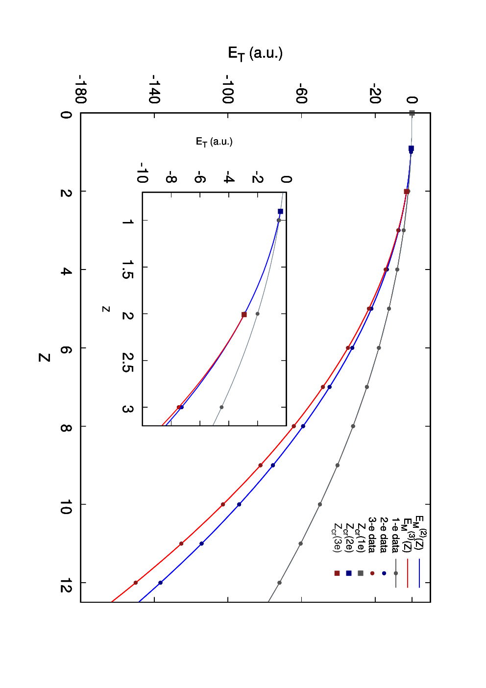
where is the distance from charge Z to th electron of mass and charge , is three-dimensional Laplacian associated with th electron, is the distance between the th and th electrons, . Thus, energy is in atomic units (a.u.). It is widely known that there exists a certain critical charge above of which, , the system gets bound forming a electron atomic ion. It is also known that for fixed the total energy of a bound state , when exists, as the function of integer charge is very smooth, monotonously-decreasing negative function which, with the growth of , is approaching to the sum of the energies of Hydrogenic ions, see for illustration Fig.1 at , which behaves as at large .
It is well known that domain of applicability of NRQED with static charge is limited due to finite-mass effects, as well as relativistic and QED effects, and many other effects. The first three effects are dominant and define the domain of applicability. For large the relativistic effects become significant and the Schrödinger equation should be replaced by the Dirac equation. In order to remain in the Schrödinger equation formalism we limit our consideration by . Hence, the Schrödinger equation with Hamiltonian (1) describes NRQED within its domain of applicability. However, non-relativistic energies emerging as eigenvalues of the Hamiltonian (1) are defined not only in the domain of applicability of NRQED but also beyond of it, . We call the ”quantum” correction to NRQED. Self-consistent solution of NRQED implies that is of the same order of magnitude as the leading order of the sum of relativistic, QED and finite mass corrections. Evidently, there are many solutions of NRQED corresponding to different with different effective potentials other than (1). It seems natural to try to find an effective theory with potential , other than (1), leading to , which allows the maximally simple exact solution. For the effective theory remains the same NRQED (1) since two-body Coulomb problem is exactly solvable with a Coulomb orbital as the exact solution; as for it will be shown that the celebrated Hylleraas function for the ground state [2] is one of the simplest exact solutions of the effective theory, see below, which reproduces . Needless to say that the knowledge of the exact solutions allows us to find perturbatively the relativistic, QED and finite-mass corrections as well as quantum correction.
In many applications, especially, in astrophysics and plasma physics we do not need high accuracies, it might well be inside of the domain of applicability of NRQED with static charges where relativistic, QED and mass effects can be neglected. Hence, it is a natural problem to find such a domain of applicability of NRQED explicitly for a few electron systems with static nuclear charge. Surely, it may depend on the quantity we study. As the first step we consider the ground state energy for 2-3 electron atomic systems which is predominantly non-relativistic. We assume that everything is already known for one-electron, hydrogen-like systems, see for review [1]. As the second step we show that the ground state energy is easily approximated, in particular, by using the generalized Majorana formula but with coefficients different from ones from 1/Z expansion, see below.
(A) For two-electron case, (H-, He, Li+ etc) with infinitely heavy charge (we call it the static approximation) the spectra of low-lying states was a subject of intense, sometimes controversial, numerical studies (usually, each next calculation had found that the previous one exaggerated its accuracy). This program had run (almost) since the inception of quantum mechanics [2] and had culminated at 2007 [3] when the problem was solved for for the ground state with overwhelmingly/excessively high accuracy ( s.d.) from physical point of view and it still continues. Recently, it was checked that the energies found in [3] are compatible with -expansion up to 12 d.d. for and 10 d.d. for , see [4]. A time ago Nakashima-Nakatsuji made the impressive calculation of the ground state energy of the 3-body problem with finite mass of nuclei [5]. It was explicitly seen that taking into account the finiteness of the nuclear mass changes in the energy (taken in a.u.) the 4th s.d. for and the 5th s.d. for . In present paper using the Lagrange mesh method (see for basics [6]) we checked and confirmed correctness of the 12 s.d. in both cases of infinite and finite nuclear masses for obtained in [3, 5]. We also (re)calculated the ground state energies in both cases of infinite and finite nuclear masses (in full geometry for the first time) for larger with accuracy of not less than 10 d.d. 1 11footnotetext: Note that for the ground state energy difference for infinite and finite nuclear mass (full geometry cases), see Table I, coincides with the sum of the first three orders in mass ratio found in [7] in 11 d.d.
Note that in early days of quantum mechanics young Ettore Majorana in his unpublished notes proposed an empirical one-parametric formula for the ground state energy (in a.u.) versus nuclear charge :
where is parameter, which can be found variationally, see, for historical account, references and discussion [8]. At that time this formula provided a reasonable description of energy; in principle, it can also permit to make the calculation of the (first) critical charge , where the ionization energy vanishes.
(B) For three-electron case (Li, Be+ etc) accurate calculations of the ground state energy for were carried out in [9] for both infinite and finite nuclear masses. We believe that, at least, 10 s.d. obtained in these calculations are confident. The effect of finiteness of the nuclear mass changes 4th - 3rd d.d. in the energy (in a.u.) when moving from small to large . For (and for infinite nuclear mass) the crosscheck of compatibility of obtained results with -expansion was also done: it was found that 5-6 d.d. in energy coincide [9]. This coincidence provides us the confidence in the correctness of a certain number of decimal digits (not less than six) which is sufficient for present purposes. Note that finite mass effects were found perturbatively, taking into account one-two terms in the expansion in electron-nuclei mass ratio.
Aim of the present paper is three-fold: (i) To localize the domain of applicability of non-relativistic QED for 2-3 electron systems with static nucleus, (ii) to construct a simple interpolating function for the ground state energy in full physics range of for which would reproduce the ground state energy with not less than twelve s.d. exactly, checking, in particular, applicability of the Majorana formula. Such a number of exact s.d. is definitely inside of domain of applicability of non-relativistic QED with static nucleus, which is usually less than 4 d.d.; (iii) to present a simple trial function for which the variational energy describes the exact ground state energy in the domain of applicability of non-relativistic QED with static nucleus with accuracy , thus, de facto it is the exact ground state NRQED wavefunction.
The paper is organized in the following way: Section I contains the analysis of theoretical data defining the domain of applicability of NRQED, in Section II the Puiseux expansion for small and the Taylor expansion for large for non-relativistic energies are presented; two-point interpolations are introduced in Section III, Section IV is dedicated to Majorana formula and its generalization, and a localization of critical charge, Section V is about polynomial interpolation of the sum of leading relativistic and QED corrections, Section VI presents the “exact” wavefunctions for the ground state in NRQED approximation for two and three electron ions and define effective theory behind NRQED.
Throughout the paper all energies are given in atomic units (a.u.). We use abbreviation s.d. for significant digits and d.d. for decimal digits throughout the text.
I Domain of Applicability
As the first step we have to collect data for the non-relativistic ground state energies available in literature for the cases of both infinite and finite nuclear masses (taking the masses of the most stable nuclei, see [12]) for two- and three-electron systems, see Table I, II, respectively. In particular, this step is necessary to evaluate the effects of finite nuclear mass to the ground state energy: what leading significant (decimal) digit in energy is influenced by finite mass effects.
(A) For (two-electron ions) we collected in Table I the most accurate data available in literature. As for the energies for they were recalculated employing the Lagrange mesh method [6] for infinite mass case and calculated for the first time for finite mass case (in full geometry), by using the concrete computer code designed for three-body studies [13, 15], where details can be consulted. In the past this method provided systematically the accuracy of 13-14 s.d. for the ground state energy of various 3-body problems, see e.g. [15]. As for the results (rounded to 13-14 s.d.) obtained in [3, 5] are also presented. All these energies were recalculated in the Lagrange mesh method and confirmed in all displayed digits at Table I. Relativistic and QED effects (excluding QED contributions) in leading approximation were obtained for the first time in [16] for , systematically they turned out negative; they were recalculated in [17] for . Taking into account the smallest in powers of terms only in [17] (excluding and including logarithmic contribution) in leading 3 s.d. we collected them in Table I, columns 5 and 6. In general, the difference between results of [16] and [17] occurred in one unit in the 3rd s.d. Eventually, we presented in column 5, Table I the modern results by [17] for and from [16] for . Taking polynomial interpolation in domain , see below Section V, where it reproduces systematically all 3 s.d., we extrapolate it to and . One can see that these effects leave unchanged the first 3-4 s.d. in the ground state energy. It defines the domain of applicability of NRQED with static nuclei for as 3-4 s.d. in the ground state energy. Let us emphasize that the special situation occurs for . As the result of extrapolation from to the sum of the leading corrections (hence, excluding logarithmic terms) is very small and positive, a.u., while this sum in [16] being of the same order of magnitude is negative a.u. It does not change our conclusion about domain of applicability of NRQED. Present authors do not know a reason of this discrepancy. To the best of our knowledge (hence, including logarithmic terms) for is not calculated. As for the correction (which including logarithmic terms) in leading approximation was estimated recently by Shabaev et al, [19], see below.
(B) For (three-electron ionic sequence) for infinite nuclear mass the results by Yan et al, [9] are mostly presented in Table II, column 2. Recently, for these results were recalculated by Puchalski et al, [10] using a more advanced variational method. This recalculation confirmed 9 d.d. in energies obtained in [9], but explicitly disagreed in consequent 10-11th d.d. Since the results [10] give lower energies than [9] we consider them as more accurate. As for finite nuclear mass case for the six d.d. only can be considered as established, except for , see [9, 18, 10].
In [11, 10] it was shown that for the sum of the leading relativistic () and QED () corrections is of the same order of magnitude as mass polarization. In particular, for the sum of the leading corrections a.u. while the mass correction a.u., being of opposite sign, see below Table II. As for the mass correction a.u. [10] increases in about with respect to , see Table II. Overall mass correction to ground state energy gives contribution to 5th s.d. in the ground state energy for , see below, Table II, column 3.
We are unaware about the analysis of both QED and relativistic corrections for other values of of the same quality as in [11, 10] for . Thus, we could only guess that for these leading relativistic and QED corrections leave unchanged 5-4-3 s.d. with growth of up to in the ground state energy in static approximation (similarly to the two-electron case) 2 22footnotetext: When this work was mostly completed, following our request the SPb University group (A.V. Malyshev, I.I. Tupitsyn and V.M. Shabaev) kindly agreed to make estimates of both relativistic and QED corrections in leading order for 3-electron ions for different [19], see Table II, column 5. We were informed that the method used is sufficiently accurate for large but it deteriorates at small . It turned out the estimates are consistent with results found in [10] for in and , respectively.. Eventually, it defines the domain of applicability of non-relativistic QED for three electron atomic systems with static nuclei as 3-4-5 s.d. in the total energy of ground state.
II Expansions
It is well known since Hylleraas [2] that at large the energy of -electron ion in static approximation admits the celebrated expansion,
| (2) |
where is the sum of energies of Hydrogenic atoms, is the so-called electronic interaction energy, which usually, can be calculated analytically. In atomic units are rational numbers. In particular, for the ground state for [20],
| (3) |
and [9],
| (4) |
respectively, where is the so-called electronic correlation energy. It was proved that the expansion (2) for has a finite radius of convergence, see e.g. [21].
In turn, at small , following the qualitative prediction by Stillinger and Stillinger [22] and further quantitative studies performed in [23], [24], there exists a certain value for which the non-relativistic ground state energy with static nuclei is given by the Puiseux expansion in a certain fractional degrees
| (5) |
where . This expansion was derived numerically using highly accurate values of ground state energy in close vicinity of obtained variationally. Three results should be mentioned in this respect for : (i) is not necessarily equal to the critical charge, , (ii) the square-root term is absent, hence at has square-root branch point with exponent 3/2 and it may define the radius of convergence of expansion (2), and, (iii) seemingly the expansion (5) is convergent. In particular, for the ground state at the first coefficients in (5) are
| (6) |
| (7) |
respectively.
III Interpolation
Let us introduce a new variable,
| (8) |
It can be easily verified that in the expansion (5) becomes the Taylor expansion while the expansion (2) is the Laurent expansion with the fourth order pole at . The simplest interpolation matching these two expansion is given by a meromorphic function
| (9) |
which we call the generalized, two point Pade approximant. Here are polynomials of degrees and , respectively
with normalization , thus, , the total number of free parameters in (9) is . It is clear that , thus . The interpolation is made in two steps: (i) similarly to the Pade approximation theory some coefficients in (9) are found by reproducing exactly a certain number of terms in the expansion at small and also a number of terms at large -expansion, (ii) remaining undefined coefficients are found by fitting the numerical data, which we consider as reliable, requiring the smallest . It is the state-of-the-art to choose and appropriately.
For both cases in (9) we choose , which is a minimal number leading to correct 12 s.d., at least, in fit of exact ground state energy, see below. It is assumed to reproduce exactly the first four terms in the Laurent expansion (2), , and the first three terms in the Puiseux expansion (5), . Thus, it leads us to the generalized, two point Pade Approximant . The remaining eight free parameters in Approximant
| (10) |
are found making fit. As for , data from Table I, obtained by Nakashima-Nakatsuji [3] and via the Lagrange mesh method [15], are fitted. While for data from Table II obtained by Yan et al [9] are used. In practice, in order to construct the Approximant we need to know the energies for eight values of only. In Table 3 the optimal parameters in for are presented. Let us emphasize that in both cases the roots of denominator in form complex-conjugated pairs with mostly negative (or slightly positive) real parts!
In general, expanding the function with optimal parameters, see Table III, around we get
| (a.u.) | Fit (10) | Fit (11) | Ansatz | |||||
|---|---|---|---|---|---|---|---|---|
| Infinite mass | Finite mass | Difference | (18) | |||||
| 1 | -0.527 751 016 544 4 | -0.527 445 881 1 | -0.527 751 016 548 | -0.5297 | -0.524 | |||
| 2 | -2.903 724 377 034 | -2.903 304 557 7 | -2.903 724 377 033 | -2.9049 | -2.900 | |||
| 3 | -7.279 913 412 669 | -7.279 321 519 8 | -7.279 913 412 665 | -7.2802 | -7.276 | |||
| 4 | -13.655 566 238 42 | -13.654 709 268 2 | -13.655 566 238 41 | -13.6554 | -13.651 | |||
| 5 | -22.030 971 580 24 | -22.029 846 048 8 | -22.030 971 580 23 | -22.0307 | -22.027 | |||
| 6 | -32.406 246 601 90 | -32.404 733 488 9 | -32.406 246 601 90 | -32.4059 | -32.402 | |||
| 7 | -44.781 445 148 77 | -44.779 658 349 4 | -44.781 445 148 7 5 | -44.7812 | -44.777 | |||
| 8 | -59.156 595 122 76 | -59.154 533 122 4 | -59.156 595 122 74 | -59.1565 | -59.152 | |||
| 9 | -75.531 712 363 96 | -75.529 499 582 5 | -75.531 712 363 93 | -75.5318 | -75.528 | |||
| 10 | -93.906 806 515 04 | -93.904 195 745 9 | -93.906 806 515 00 | -93.9071 | -93.903 | |||
| 11 | -114.281 883 776 1 | -114.279 123 929 1 | -114.281 883 776 0 | -114.2824 | -114.278 | |||
| 12 | -136.656 948 312 7 | -136.653 788 023 4 | -136.656 948 312 6 | -136.6577 | -136.653 | |||
| (a.u.) | Fit (10) | Fit (11) | Ansatz | |||||
|---|---|---|---|---|---|---|---|---|
| Infinite mass | Finite mass | Difference | (18) | |||||
| 20 | -387.657 233 833 2 | -387.651 875 961 4 | -387.657 233 834 0 | -387.6604 | -387.653 | |||
| 30 | -881.407 377 488 3 | -881.399 778 896 1 | -881.407 377 492 6 | -881.4142 | -881.403 | |||
| 40 | -1 575.157 449 525 6 | -1575.147 804 148 0 | -1 575.157 449 535 | -1575.1684 | -1575.153 | |||
| 50 | -2 468.907 492 812 7 | -2468.895 972 259 1 | -2 468.907 492 828 | -2468.9230 | -2468.903 | |||
For infinite mass case (column 2), underlined digits remain unchanged due to finite-mass effects (after its rounding), digits in bold reproduced by fit (10) (after rounding). Last column represents the variational energies obtained with Anzatz (21)-(26).
Leading relativistic+QED corrections (for infinite mass case) for marked (†) from [11, 10], marked by (⋆) from [19], see also [36]; for the estimates for leading relativistic+QED corrections (for infinite mass case), column 5, from [19].
| (a.u.) | Interpolation | Fit (10) | Fit (11) | Ansatz | ||||
|---|---|---|---|---|---|---|---|---|
| Infinite mass | Finite mass | Difference | (17) | (21)-(26) | ||||
| 3 | -7.478 060 323 650 | -7.477 451 884 70 | (⋆) | -7.478 060 323 651 | -7.495 | -7.455 | ||
| (†) | -7.478 060 323 91 | -7.477 452 121 22 | ||||||
| -7.477 452 048 02 | ||||||||
| 4 | -14.324 763 176 465 | -14.323 863 441 3 | -14.324 763 176 47 | -14.340 | -14.271 | |||
| (†) | -14.324 763 176 78 | -14.323 863 713 6 | ||||||
| -14.323 863 687 1 | ||||||||
| 5 | -23.424 605 720 96 | -23.423 408 020 3 | -23.424 605 720 96 | -23.436 | -23.330 | |||
| -23.423 408 350 5 | ||||||||
| 6 | -34.775 511 275 63 | -34.773 886 337 7 | -34.775 511 275 63 | -34.782 | -34.633 | |||
| -34.773 886 826 3 | ||||||||
| 7 | -48.376 898 319 14 | -48.374 966 777 1 | -48.376 898 319 12 | -48.380 | -48.182 | |||
| -48.374 967 352 1 | ||||||||
| 8 | -64.228 542 082 70 | -64.226 301 948 5 | -64.228 542 082 71 | -64.229 | -63.967 | |||
| -64.226 375 998 3 | ||||||||
| 9 | -82.330 338 097 30 | -82.327 924 832 7 | -82.330 338 097 35 | -82.328 | -81.993 | |||
| 10 | -102.682 231 482 4 | -102.679 375 319 | -102.682 231 482 4 | -102.678 | -102.243 | |||
| 11 | -125.284 190 753 6 | -125.281 163 823 | -125.284 190 753 6 | -125.279 | -124.730 | |||
| 12 | -150.136 196 604 5 | -150.132 723 126 | -150.136 196 604 5 | -150.131 | -149.440 | |||
| 13 | -177.238 236 560 0 | -177.234 594 529 | -177.238 236 560 0 | -177.233 | -176.315 | |||
| 14 | -206.590 302 212 3 | -206.586 211 017 | -206.590 302 212 3 | -206.585 | -205.507 | |||
| 15 | -238.192 387 694 1 | -238.188 129 642 | -238.192 387 694 2 | -238.188 | ||||
| 16 | -272.044 488 790 1 | -272.039 780 017 | -272.044 488 790 1 | -272.042 | ||||
| 17 | -308.146 602 395 3 | -308.141 728 192 | -1.06 | -1.06 | -308.146 602 395 3 | -308.146 | ||
| 18 | -346.498 726 173 7 | -346.493 932 364 | -1.35 | -1.35 | -346.498 726 173 7 | -346.500 | ||
| 19 | -387.100 858 334 6 | -387.095 367 736 | -1.69 | -1.69 | -387.100 858 334 6 | -387.105 | ||
| 20 | -429.952 997 482 8 | -429.947 053 487 | -2.10 | -2.10 | -429.952 997 482 8 | -429.961 | ||
| parameters | ||
|---|---|---|
| -0.40792489 | -2.934281 | |
| -1.7720945736 | -4.985319466822 | |
| -5.09227274076 | -12.51820588130 | |
| -11.4229111014 | -14.24645657801 | |
| -16.6866531073 | -15.83837203461 | |
| -28.2878912031 | -15.74077387390 | |
| -21.7247609889 | -8.13280408452 | |
| -31.4514043213 | -7.836711216798 | |
| -10.1253004761 | -1.490328878341 | |
| -13.4157573972 | -1.485186602328 | |
| 1.0 | 1.0 | |
| 4.34416878449 | 1.698991837122 | |
| 9.72923652871 | 3.110764743151 | |
| 15.5576492283 | 2.861781316187 | |
| 10.1253004761 | 1.324736780747 | |
| 13.4157573972 | 1.320165868736 |
| parameters | ||
|---|---|---|
| -0.407924 | -2.934281 | |
| 0.0 | 0.0 | |
| -1.184891 | -3.485218 | |
| -0.000027 | -0.002469 | |
| -1.0 | -9/8 |
In Table I and II the results of interpolations for and are presented, respectively. In general, for the difference in energy occurs systematically in 13rd s.d. or, sometimes, in 14th s.d. for all range of studied, except for for , where it occurs in 12th s.d.
The analysis of relativistic and QED corrections for two-electron system performed for in [17, 7], see Table I, shows that they are small or comparable with respect to the mass polarization effects for and then become larger (and dominant) for . Note that the relativistic and QED corrections systematically are of opposite sign.
Similar analysis of relativistic and QED corrections of three-electron system, performed for in [11, 10], shows that they contribute to the 1st s.d. in the energy difference between infinite and finite mass cases. For both cases of 2- and 3-electron systems the question about the order of relativistic and QED effects for large needs to be investigated. We can only guess that for both systems the domain of applicability of static approximation for any is limited by 3 s.d. in the ground state energy.
Interestingly, the simplest interpolation (which is in fact the terminated Puiseux expansion) with two fitted parameters ,
| (11) |
with other parameters taken from Table 4 3 33footnotetext: Note that the parameter is small, hence, the term does not play a significant role in description of energy dependence at and reproduces 3-4 s.d. in ground state energy in static approximation for both systems in physics range of , see Tables I,II . These 3-4 s.d. remain unchanged if all finite-mass, relativistic and QED effects are taken into account. It implies the exact reproduction of the domain of applicability of non-relativistic QED in static approximation for the ground state total energy!
IV Majorana Formula and the (first) critical charge
Originally, the Majorana formula 4 44footnotetext: Recently, this formula was found, in fact, in unpublished and unknown till recently notes by E Majorana circa 1930, see e.g. Eq.(22) in [8] and references therein
| (12) |
was written for the ground state energy of two-electron system in static approximation as the variational energy for the trial function (i), then it was re-interpreted as the first three terms of -expansion, cf. (2) (ii) and then the parameter was set free to be chosen to get the best description of experimental data for Helium atom, , [8] (iii) 5 55footnotetext: For one-electron case, , the Majorana formula at and is exact. In fact, at . None of these three considerations (i)-(iii) had led to accurate description of data being limited to 1-2 s.d. and, sometimes, to 3 s.d., see Table 5. Note since E Majorana was likely the first who treated as continuous parameter, those three considerations provided for the first time the values of the (first) critical charge , where the one-electron ionization energy vanishes , see Table 5. The situation changes dramatically if parameter or two parameters are varied to get the best fit of data in the whole domain : the Majorana formula reproduces consistently, at least, 3-4 s.d. in the ground state energy leading to the exact NRQED energies at in a way similar to (11) (with parameters from Table 4) 6 66footnotetext: Note that although fitted parameters are very close to the second-third coefficients in -expansion for two-electron systems (3), but different. Namely, due to the difference we are able to get high quality approximation. In this case the Majorana formula (12) gives rather accurate value of the first critical charge :
see Table 5 (3rd line), which is in good agreement with the value of the critical charge predicted by the Approximants given by (11) or by (10) as well as with the exact result [14, 15] 7 77footnotetext: Energy at found in [14, 15] is reproduced by Approximant (10) in 10 s.d.(!), the energy difference is , cf. Table I. Eventually, the Majorana formula with fitted coefficients can be considered as accurate interpolation of the ground state energy curve for two-electron system on Fig. 1. Note that -expansion can be constructed for any excited state and it always has the form (2). By taking a linear superposition of the first three terms we will arrive at the Majorana type formula (12). By keeping the coefficient equal to one found in -expansion and fitting the coefficients we should get a reasonable description of -dependence of the energy of an excited state. It will be checked elsewhere.
| Approximation | parameters | |||
| Majorana formula (12) | 1.066 942 | |||
| 0.906 982 | ||||
| 0.913 617 | ||||
| Generalized Pade | (11) (see Table 4 ) | 0.910 007 | ||
| (10) (see Table 3 ) | 0.911 028 22 | |||
| Exact [14, 15] (rounded) | 0.911 028 22 | |||
It is natural to try to explore the Majorana formula (12) to describe the -dependence of the ground state energy of three-electron system, , with fixed and fitting . Straightforward fit shows that the Majorana formula reproduces at least 3-4 s.d. in the ground state energy leading to the exact NRQED energies at in a way similar to (11) (with parameters from Table 4) 8 88footnotetext: Note that although fitted parameters are very close, but are slightly different, to the second-third coefficients in -expansion for three-electron systems (4). Namely, due to the difference we are able to get high quality approximation. In this case the Majorana formula (12) gives a reasonable value of the first critical charge
see Table 6. For the case of generalized Pade approximations (11) and (10) the predicted first critical charge coincides with the second critical charge [23]: it is the minimal nuclear charge for ground state function becomes non-normalizable.
| Approximation | parameters | |||
| Majorana formula (12) | 2.256 | |||
| Generalized Pade | (11) (see Table 4 ) | 2.009 | ||
| (10) (see Table 3 ) | 2.009 | |||
Eventually, one can state that the Majorana formula with fitted coefficients can be considered as accurate interpolation of the ground state energy curve for three-electron system in NRQED approximation, see Fig.1.
Apparently, -expansion can be constructed for any excited state of three electron system and it has the form (2). By taking a linear superposition of the first three terms we will arrive at the Majorana type formula (12). Seemingly, by fitting the coefficients with taken from -expansion we should get a reasonable description of -dependence of the energy of an excited state of system. It will be checked elsewhere.
V Approximating the sum of leading relativistic and QED corrections versus
In previous Section it was shown that the second degree polynomial in (Majorana formula (12)) approximates accurately NRQED ground state energies for Helium like and Lithium like systems. We conjectured that it remains true for the energy of any excited state and for other atom-like systems with . It is interesting to try to approximate the sum of leading relativistic and QED corrections of orders and , respectively, (excluding and including logarithmic contributions); see e.g. [16, 17], presented in columns 5 and 6 in Tables I (and II) for different . It does not look as a simple task since from to it changes in six orders of magnitude(!), see Table I .
Following standard formulas for the sum in leading order, see e.g. [16], at large , it behaves like , if -dependence is neglected. Hence, as interpolating function we choose naively a polynomial in of degree 4,
| (13) |
For the Helium-like sequence we choose 11 integer points and make fit of 5 parameters in (13) with goal to reproduce all 3 s.d. in (excluding and including logarithmic contributions ) printed in Table I, column 5 and 6. This goal is achieved for both 9 99footnotetext: Except for , where for unclear reason the deviation in one unit in the 3rd s.d. was seen, where we predict at , and for total . For larger the value of is described with relative accuracy , see Table 1 (continuation). Final expression for interpolating polynomial reads,
| (14) |
while for the total relativistic and QED correction in leading approximation it is,
| (15) |
For Lithium-like sequence we choose 9 integer points and make fit of 5 parameters in (13) with the first goal to reproduce all three s.d. in estimates of due to [19], printed in Table II column 5. It can be easily done and the interpolating polynomial is presented by
| (16) |
It reproduces estimates in all points in except for where it differs in one unit in the 3rd figure. It implies that the results for approximate method used in [19] are modeled by (16) with high accuracy. As the second goal we want to approximate the known reliable results for for [11, 10] and [19]. Surprisingly, the polynomial,
| (17) |
reproduces results in 3 s.d. for and , see Table II, column 6. Deviations which occur for measure an inaccuracy of the method used in [19].
VI Variational energies vs exact ones
VI.1 Two-electron case
In 1929 E Hylleraas in his celebrated paper [2] proposed to use for Helium type system the exponentially correlated trial function in the form of symmetrized product of three (modified by screening) Coulomb Orbitals (cf. formula (13) in Ref.[2]),
| (18) |
with three variational parameters , here is permutation operator . Many years after, Calais-Löwdin [27] demonstrated that all integrals involved to the variational calculations are intrinsically 3-dimensional in variables (for discussion see [28]) and they can be evaluated analytically. Eventually, the variational energy is a certain rational function of parameters . Hence, the procedure of minimization of the variational energy is essentially algebraic and can be easily performed. On Fig.2 the optimal parameters vs the nuclear charge are presented - they are smooth, slow-changing functions. At tends to infinity the -parameters approach slowly to one, , and , while asymptotically, at the function (18) (in appropriate variables) becomes the product of two ground state Coulomb orbitals. Making concrete calculations for different values of one can see that the variational energy coincides systematically with exact NRQED energies in 4-3 s.d. while at , in fact, it differs in the 3rd d.d.! Thus, the simple trial function (18) describes the energy in the domain of applicability of NRQED in static approximation. Overall quality of the trial function (18) can be ”measured” by how accurately it reproduces the electron-nucleus cusp parameter (the residue in Coulomb singularity at or ) by , see Fig.2. If at small the difference is of order 10, then it reduces to 0.01 at and tends to zero at large . For reasons unclear to the authors the electron-electron cusp at is not well-reproduced, it differs in about 50. It means that the variational trial function does not behave correctly in vicinity of , which however does not influence the quality of variational energy. This question will be studied elsewhere.
Two-electron case: effective potential
Taking trial function (18) with optimal parameters one can calculate a potential for which this function is the exact ground state function
| (19) |
which we will call the effective potential for two-electron problem. It can be easily checked that this potential reproduces Coulomb singularities at . One can define the effective theory with Hamiltonian,
| (20) |
for which the ground state energy coincides with NRQED energy in its domain of applicability.
Taking as the zero approximation in Non-Linearization Procedure with as unperturbed potential, one can develop the convergent perturbation theory w.r.t. difference between the original potential (1) and (19), see for review [29]. The sum of the first two terms coincides with the variational energy with trial function . It is evident that the next correction is the first quantum correction to NRQED; in general, it changes the 3rd (and higher) d.d. in the variational energy. This procedure allows us to calculate quantum corrections to NRQED with static nuclei. These corrections, of course, can be calculated indirectly using variational method by taking more complicated trial functions than (18), in particular, their linear superpositions, see e.g. [30].


VI.2 Three-electron case.
For Lithium-type system let us take a variational trial function (for the total spin 1/2) in the form
| (21) |
where is the spin eigenfunction, is the three-particle antisymmetrizer
| (22) |
and is the explicitly correlated orbital function
| (23) |
see e.g. [31], where and are non-linear variational parameters. Here, represents the permutation , and stands for the permutation of into . In total, (21) contains six all-non-linear variational parameters. The function (21) is a properly anti-symmetrized product of (modified by screening) Coulomb orbitals and the exponential correlation factors .
There are two linearly independent spin functions of mixed symmetry:
| (24) |
and
| (25) |
where , are spin up, spin down eigenfunctions of -th electron, respectively. For simplicity, the spin function in (21) is chosen as
| (26) |
(see [31]), where is a variational parameter. It implies that the coordinate (orbital) functions in front of are the same. Eventually, the trial function is a linear superposition of twelve terms, it contains 7 free parameters.
The variational energy is given by the ratio of two nine-dimensional integrals. In relative space coordinates the integration over three angles describing overall orientation and rotation of the system are easily performed analytically. We end up with six-dimensional integrals over the relative distances (for the general discussion see [28]). It was shown a long ago by Fromm and Hill [32] that these integrals can be reduced to one-dimensional ones (!) but with integrands involving dilogarithm functions. The analytic properties of the resulting expressions for integrands are found to be unreasonably complicated (see e.g. [33]) for numerical evaluation. For that reason, the method we used is direct numerical evaluation of the original six-dimensional integrals.
The results of variational calculations are shown in Table 2, last column for . Variational parameters vs are presented in Fig. 4, they are smooth, slow-changing functions. Parameter being small at grows with reaching sufficiently large value at . It indicates the importance of the contribution emerging from the second spin function (25) for large . It might be considered as the indication that the condition (26) should be relaxed and the orbital functions should be different,
| (27) |
see (21), where ’s are given by (23). Now this trial function depends on 13 free parameters. Immediate calculation shows a significant improvement in variational energy even for : -7.471 a.u. vs -7.455 a.u., see Table II [34].
It is easy to check that variational energies reproduce not less than 99.9 of the exact non-relativistic energies, hence, the NRQED energies in static approximation. Moreover, relaxing condition (26), thus, assuming that both orbital functions are different being the type (23), should increase accuracy. Note that the overall quality of the trial function (21)-(26) is reflected in accurate reproduction of electron-nuclear cusp parameter 2.953 [31] at while the exact one is equal to 3, thus, it deviates in about 2. Using the function (27) the value of electron-nuclear cusp parameter gets even better 2.991 [34].
Similar to two-electron case for reasons unclear to the authors the electron-electron cusp at is not well-reproduced being smaller in about 50 . It means that the variational trial function does not behave correctly in vicinity of , which it does not influence the quality of variational energy. This question will be studied elsewhere.

(a)

(b)

(c)
Three-electron case: effective potential
Taking trial function (21) with optimal parameters one can calculate a potential for which this function is the exact ground state function
| (28) |
cf. (19), which we will call the effective potential for three-electron problem. It can be easily checked that this potential reproduces Coulomb singularities at . One can define the effective theory with Hamiltonian,
| (29) |
for which the ground state energy coincides with NRQED energy in its domain of applicability.
Conclusions
Concluding we state that a straightforward interpolation between small and large in a suitable variable (8) based on a meromorphic function (10) leads to accurate description of 12-13-14 s.d. of the non-relativistic ground state energy of both the Helium-like and Lithium-like ions in static approximation, thus, for and states, respectively, for . Even at critical charge for Helium-like system it provides 10 s.d. in ground state energy correctly. In general, such an outstanding accuracy provided by (10) leads to a hint that the Puiseux expansion (5) at has finite radius of convergence while the expansion at is a Taylor expansion with finite radius of convergence as well. It also indicates that the radius of convergence of -expansion is defined by .
It is worth noting that the quality of approximation increases substantially with the growth of in generalized two-point Pade approximation (9): at it gives accuracy of 3-4 s.d. in the ground state energy for all studied, while at the accuracy increases to 7-8 s.d. and, eventually, at it gives the above-mentioned accuracy 12-13-14 s.d. It seems natural to assume that the similar interpolation has to provide high accuracy for the energies of excited states of above systems and even for other many-electron atomic systems. It will be presented elsewhere [25].
It has to be emphasized that at present for Helium atom the experimental accuracy is of the order in relative units [35] (for discussion see [7]). Theoretically, the contributions of the order of for excited states) are unknown. It seems important to know to what significant digit in ground state energy this correction will give contribution. It might be that this correction as well as non-QED contributions e.g. hadronic loops may influence 9-10th significant digit in energy. Let us emphasize that our interpolation provides non-relativistic energies well beyond the present accuracy of both experimental and theoretical data.
Note that similar interpolation works very well for simple diatomic molecules H, H2, He and in Born-Oppenheimer approximation matching perturbation theory at small internuclear distances and multipole expansion with instanton-type, exponentially-small contributions at large distances (as for the first three systems). It provides 4-5-6 s.d. at potential curves depending on internuclear distances and eventually not less than 5-6 s.d. for spectra of existing rovibrational states [26].
Making detailed analysis of finite mass corrections, QED and relativistic effects for the ground state energy of 2- and 3-electron ions for we localized the domain of applicability of NRQED in static approximation. This domain is limited by 4-3 s.d. in the ground state energy for both systems. Surprisingly, this domain is described accurately by a 4th degree polynomial (without linear term) in variable , where is the 2nd critical charge [24]. This domain can also be fitted by the Majorana formula - the 2nd degree polynomial in (12) with two free parameters, while - the coefficient in front of term - is kept fixed and equal to the sum of the (ground state) energies of 2(3)-Hydrogen atoms - with similar accuracies of 4-3 s.d.! Remarkably, the first 3 s.d. in the leading approximation of the sum of relativistic and QED corrections are systematically described by 4th degree polynomial in Z for for Helium-like and for for Lithium-like systems.
Note that the Majorana formula (12) (as well as generalized two-point Pade approximations) allows us to calculate the (first) critical charge in reasonably accurate way. Adding to the Majorana formula the term slightly improves the quality of approximation at small integer but allows to describe correctly the energy in vicinity of the first (second) critical charge . Striking fact is all three curves shown on Fig.1 are, in fact, parabolas (up to width of drawing line)!
It seems interesting to check applicability of Majorana formula for NRQED with finite mass nuclei. In order to do it we calculated for the first time in full geometry the non-relativistic ground state energy of two-electron atomic system for in Lagrange mesh method with accuracy not less than 10 d.d. It complements the results by Nakashima-Nakatsuji [5] for . These results are displayed in the 3rd column of Table I. As for 3-electron systems one-two leading finite-mass corrections are included into the ground state energy, see Table II, 3rd column. The sum of relativistic and QED corrections in leading approximation remains almost unchanged. Domain of applicability of NRQED is again limited to 3-4 s.d. In both cases of two and three electron sequences the Majorana formula - the second degree polynomial in - continues to describe domain of applicability of NRQED with slightly changed coefficients, see Table V and VI.
Interestingly, making a generalization of the Slater determinant method by including inter-electronic correlations in exponential form, thus, taking a trial function in the form of (anti)-symmetrized product of three (six) modified-by-screening Coulomb orbitals for two-(three-) electron system (they can be called generalized Hylleraas functions), respectively, allows us to reproduce of the ground state energy from small up to . Of course, it requires a careful minimization with respect to screening (non-linear) parameters. In other words, the obtained variational energy, in fact, coincides with exact energy in domain of applicability of NRQED with (in)finitely-heavy nuclei. This observation hints that such a generalized Slater determinant method might be successful for other atomic and molecular systems. It will be checked elsewhere.
Acknowledgements.
A.V.T. is grateful to Physics Department of Stony Brook University and Simons Center (Stony Brook, USA) where some parts of the present work were carried out. J.C.L.V. thanks PASPA grant (UNAM, Mexico) and the Centre de Recherches Mathématiques, Université de Montréal, Canada for the kind hospitality while on sabbatical leave during which this work was initiated. H.O.P. wants to express a deep gratitude to ICN-UNAM (Mexico), where the essential part of the present work was done during his numerous visits. A.V.T. thanks M.I. Eides, V.M. Shabaev and V.A. Yerokhin for useful remarks. The authors thank G.W.F. Drake for important discussions and clarifications. Most of calculations associated with generalized Slater determinants - generalized Hylleraas functions were carried out on 120-processor cluster KAREN (ICN-UNAM, Mexico). In the last stage the research was supported partially by CONACyT grant A1-S-17364 and DGAPA grant IN108815 (Mexico). The authors express deep gratitude to two anonymous referees for careful reading of the manuscript, constructive suggestions and critical remarks – all that helped to improve the presentation.References
- [1]
M. I. Eides, H. Grotch and V. A. Shelyuto,
Theory of light hydrogen-like atoms, Physics Reports 342 63-261 (2001) - [2]
E.A. Hylleraas,
Neue Berechnung der Energie des Heliums im Grundzustande, sowie des tiefsten Terms von Ortho-Helium,
Z. Phys. 54 347-366 (1929) (in German);
English translation: Quantum chemistry: classic scientific papers, translated and edited by H Hettema, Singapore; London: World Scientific, 2000, pp 104-121. - [3]
H. Nakashima, H. Nakatsuji,
Solving the Schrödinger equation for helium atom and its isoelectronic ions with the free iterative complement interaction (ICI) method,
J. Chem. Phys. 127, 224104 (2007) - [4]
A.V. Turbiner, J.C. López Vieyra,
On expansion, critical charge for two-electron system and the Kato theorem,
Can. Journ. of Phys. 94 249-253 (2016) - [5]
H. Nakashima, H. Nakatsuji,
Solving the electron-nuclear Schrödinger equation of helium atom and its isoelectronic ions with the free iterative-complement-interaction method
J. Chem. Phys. 128, 154107 (2008) - [6]
D. Baye,
Lagrange-mesh method,
Phys. Repts. 565, 1 - 107 (2015) - [7]
K. Pachucki, V. Patkos and V.A. Yerokhin,
Testing fundamental interactions on the helium atom,
Phys. Rev. A95 (2017) 062510 - [8]
S. Esposito, A. Naddeo,
Majorana Solutions to the Two-Electron Problem
Found. Phys. 42 (2012) 1586 - 1608 - [9]
Z.C. Yan, M. Tambasco, and G.W.F. Drake,
Energies and oscillator strengths for lithiumlike ions,
Phys. Rev. A57, 1652 (1998) - [10]
M. Puchalski and K. Pachucki,
Relativistic, QED, and finite nuclear mass corrections for low-lying states of Li and ,
Phys. Rev. A78, 052511 (2008) - [11]
Z.C. Yan and G.W.F. Drake,
Bethe logarithm and QED shift for lithium,
Phys. Rev. Lett. 91, 113004 (2003) - [12]
G. Audi, A.H. Wapstra, and C. Thibault,
Nucl. Phys. A729, 337 (2003) - [13]
M. Hesse and D. Baye,
Lagrange-mesh calculations of the ground-state rotational bands of the and
molecular ions,
J. Phys. B36 139 (2003) - [14]
C. S. Estienne, M. Busuttil, A. Moini and G. W. F. Drake,
Critical Nuclear Charge for Two-Electron Atoms,
Phys. Rev. Lett. 112, 173001 (2014) - [15]
H. Olivares-Pilón and A.V. Turbiner,
Nuclear critical charge for two-electron ion in Lagrange mesh method,
Phys. Lett. A379, 688 (2015) - [16]
G. W. F. Drake,
Theoretical energies for the and 2 states of the helium isoelectronic sequence up to ;
Can. Journ. of Phys. 66 586-611 (1988);
for update see webpagehttp://drake.sharcnet.ca/mediawiki/index.php/Dr._Gordon_Drake%27s_Research_Group - [17]
V.A. Yerokhin and K. Pachucki,
Theoretical energies of low-lying states of light helium-like ions,
Phys. Rev. A81 (2010) 022507 - [18]
M. Godefroid, C. Froese Fischer and P. Jönsson,
Non-relativistic variational calculations of atomic properties in Li-like ions: Li I to O VI,
Journ. of Phys. B 34, 1079 (2001) - [19] A.V. Malyshev, I.I. Tupitsyn, and V.M. Shabaev (private communication)
- [20]
J.C. López Vieyra, A.V. Turbiner,
On expansion for two-electron system,
arXiv: 1309.2707v3 [quant-ph], pp.7 (Sept-Dec 2013) - [21]
T. Kato,
Perturbation Theory for Linear Operators,
2nd edition, Springer-Verlag: Berlin-Heidelberg-New York p. 410-413 (1980) - [22]
F.H. Stillinger,
Ground energy of two-electron atoms,
J. Chem. Phys. 45, 3623-3631 (1966);
F.H. Stillinger, D.K. Stillinger,
Non-linear variational study of perturbation theory for atoms and ions,
Phys. Rev. 10, 1109 (1974) - [23]
A.V. Turbiner, N.L. Guevara,
Heliumlike and lithiumlike ionic sequences: Critical charges,
Phys. Rev. A84 (2011) 064501 (4pp) - [24]
A.V. Turbiner, J.C. López Vieyra and H. Olivares Pilón,
Three-body quantum Coulomb problem: Analytic continuation,
Mod. Phys. Lett. A 31 (2016) 1650156 - [25]
A.V. Turbiner, J.C. López Vieyra, H. Olivares Pilón, J.C. del Valle and D.J. Nader,
Ground state energy in quantum mechanics: Interpolating between weak and strong coupling regime (work in progress) - [26]
H. Olivares Pilón, and A.V. Turbiner,
, HeH and : approximating potential curves, rovibrational states,
Ann. of Phys. 393 (2018) 335-357;
Towards the theory of Potential Energy Curves for diatomic molecular ions: He case,
ArXiv: 1904.066, pp.17 (April 2019) - [27]
J.-L. Calais and P.-O. Löwdin,
A Simple Method of Treating Atomic Integrals Containing Functions of ,
J. Mol. Spectr. 8, 203-211 (1962) - [28]
A. V. Turbiner, W. Miller Jr and M.A. Escobar Ruiz,
Journal of Physics A50 (2017) 215201;
Journ of Math Physics A59 (2018) 022108;
Journal of Physics A51 (2018) 205201 - [29]
A. V. Turbiner,
The Problem of Spectra in Quantum Mechanics and the ’Non-Linearization’ Procedure,
Soviet Phys. - Usp. Fiz. Nauk. 144, 35-78 (1984),
Sov. Phys. Uspekhi 27, 668-694 (1984) (English Translation). - [30]
V.I. Korobov,
Coulomb variational bound state problem: variational calculation of nonrelativistic energies,
Phys. Rev. A 61 (2000) 064503 - [31]
N.L. Guevara, F.E. Harris and A.V. Turbiner,
An Accurate Few-Parameter Ground State Wave Function for the Lithium Atom,
Int. Journ. Quant. Chem, 109, 3036-3040 (2009) - [32]
D.M. Fromm, R.N. Hill,
Analytic evaluation of three-electron integrals,
Phys. Rev. A 36, 1013-1044 (1987) - [33]
F.E. Harris,
Analytic evaluation of three-electron atomic integrals with Slater wave functions,
Phys. Rev, A 55, 1820-1831 (1997) - [34] J.C. del Valle and D.J. Nader (private communication)
- [35]
S.Sturm, F. Köhler, J. Zatorski, et al,
High-precision measurement of the atomic mass of the electron
Nature 506, 467–470 (2014)