gen.parRep: a first implementation of the Generalized Parallel Replica dynamics for the long time simulation of metastable biochemical systems
Abstract
Metastability is one of the major encountered obstacle when performing long molecular dynamics simulations,
and many methods were developed to address this challenge.
The “Parallel Replica”(ParRep) dynamics is known for allowing to simulate very long
trajectories of metastable Langevin dynamics in the materials science community,
but it relies on assumptions that can hardly be transposed to the world of biochemical simulations.
The later developed “Generalized ParRep” variant solves those issues, but it was not applied to
significant systems of interest so far.
In this article, we present the program gen.parRep, the first publicly available
implementation of the Generalized Parallel
Replica method
(BSD 3-Clause license), targeting
frequently encountered metastable biochemical systems, such as conformational equilibria or
dissociation of protein–ligand complexes.
It will be shown that the resulting C++ implementation exhibits a strong linear scalability, providing up to 70% of the maximum possible
speedup on several hundreds of CPUs.
Keywords:
Molecular simulations; Langevin dynamics; Quasi-stationary distributions; Metastability; Protein–Ligand dissociation; High Performance ComputingProgram Title:
gen.parRep
Licensing provisions:
BSD 3-clause
Programming language:
C++ (mostly), C and Lua
Nature of problem:
Molecular dynamics simulations of chemical and biological systems usually encounter the problem of
metastability, because of the timescale separation between the time discretization step used for dynamics
and the usual mean time between conformational changes. The use of Accelerated dynamics [1] methods is
usually necessary in order to address this challenge.
Solution method:
The Generalized Parallel Replica method [2] accelerates the exit from metastable states, providing a linear speedup of , being the
number of replicas of the system running in parallel. This C++ implementation, the first available so far, exhibits a strong linear scaling
on hundreds of CPUs, therefore ready for production studies on High Performance Computing (HPC) machines.
Additional comments:
Git repository:
https://gitlab.inria.fr/parallel-replica/gen.parRep
References
- [1] Lelièvre, T., Eur. Phys. J. Spec. Top. (2015) 224, DOI: 10.1140/epjst/e2015-02420-1
- [2] Binder, A. et al., Journal of Computational Physics (2015) 284; DOI: 10.1016/j.jcp.2015.01.002
1 Introduction
Molecular dynamics (MD) simulations are nowadays of a common use for simulating large and complex biological or chemical systems [1]: the continuous increase of the available computing power, together with the development of stable and accurate deterministic or stochastic sampling strategies, made possible the emergence of computer based, in silico drug design strategies [2, 3, 4]. However, a commonly encountered obstacle while performing MD simulation is the timescale separation between the fastest conformational changes — usually vibrations occurring at the femtoseconds (fs) level — and the slowest one, occurring from the nanosecond (ns) to second (or more) timescale; one may use various coarse grained [5, 6] approaches in order to reach such large simulation time, however this usually implies to sacrifice the accurate description of fast processes, such as non-bonded donor–acceptor interactions, playing a key role in biological interactions [7, 8]. The existence of metastable regions in the configurational space, separated by high potential energy or entropy barriers, is the main origin of this timescale separation, and the simulation time required for observing a transition from such a region to another one can quickly become intractable by the use of direct numerical simulations.
A large amount of methods were developed to address the challenge of metastability in MD simulations. When it is assumed that both the starting and the ending metastable regions (let us denote them by and ) are known, one can consider that most of the methods fall within one of the two following categories: local search methods start from an initial guess path connecting and , and will optimize it until convergence to an optimal path, for example characterized by a minimal potential or free energy profile: the nudged elastic band method [9], the string method [10], the max flux approach [11], the weighted ensemble methods [12, 13], or the transition path sampling method [14] (which is actually a path sampling method starting from the initial guess, but not an optimization method); the second category consists in global search methods where the ensemble of all the possible paths between and is sampled without any initial guess, and it includes adaptive multilevel splitting methods [15, 16, 17, 18], transition interface sampling [19], forward flux sampling [20] or milestoning techniques [21, 22, 23, 24, 25, 26, 27].
A. F. Voter and coworkers also proposed another class of methods, the Accelerated Dynamics methods [28, 29, 30, 31, 32]: the Parallel Replica (ParRep) method (and the derived ParSplice algorithm) [33, 34, 35, 36], the hyperdynamics method [37, 38], and the temperature accelerated dynamics method [39]. They all rely on the Transition State theory and kinetic Monte Carlo models, and the aim of these algorithms is to efficiently generate the succession of jumps between metastable regions in a statistically consistent way compared to the reference Langevin dynamics.
The ParRep method was later formalized [40], and it was shown that the notion of quasi-stationary distribution (QSD) [41, 42] is the mathematical foundation at its heart: this revealed one of the possible weaknesses of the algorithm, where it is assumed that the (user defined) time required for converging to the QSD is the same for all the metastable regions. While this assumption may be reasonable for materials science, this cannot be transposed to the chemical configurational space, where the large variety of possible interactions and steric exclusions usually results in a rough energy landscape, characterized by both an extremely large number of energy minima, and the presence of super basins of attraction (usually referred to as “funnels”). The Generalized Parallel Replica (Gen. ParRep ) [43] method addresses this issue by estimating during the simulation if convergence to the QSD is obtained; however, while this can possibly extend the range of application of ParRep to any biochemical system which can be studied via MD, no implementation has been designed and released so far.
This article describes the first publicly available implementation of Gen. ParRep ,
specially targeting metastable biochemical systems.
After a description of the methods in Section 2,
the novelty of the software implementation is detailed in Section 3;
two study cases are later investigated in Section 4, the conformational equilibrium
of the alanine dipeptide (subsection 4.1), and the dissociation of the
protein–ligand complex FKBP–DMSO (subsection 4.2).
It will be shown in both cases that the Gen. ParRep algorithm can be used for accurately
sampling the state-to-state dynamics, and in particular the state-to-state transition times;
furthermore evidences that the
software exhibits a strong linear scaling will be reported: when
running over hundreds of CPUs, one gets speedups of up to 70 % of the maximum possible linear speedup.
2 Methods
2.1 Langevin dynamics
Let us consider a stochastic process ( representing the phase space), where and denote the positions and momenta of the particles at time . The stochastic process follows the Langevin dynamics:
| (1) |
where is the inverse temperature, is the mass matrix, is a function associating to a given configuration a potential energy , is the damping parameter, and a -dimensional Brownian motion.
The Langevin dynamics on the -dimensional potential energy surface is likely to consist in a succession of “entry then exit” events from wells (or groups of wells) progressively discovered by the process , and one can expect that the time spent within a well before it hops to another one will be far more large that the discretization timestep : it is therefore necessary to design an alternative approach to the computationally expansive direct simulation in order to address this problem of metastability.
2.2 States and metastability
Let us introduce the ensemble of metastable states . These are typically defined in terms of positions only
(and not velocities). In the original ParRep algorithm [33, 35], these states are defined as the
basins of attraction of the local minima of for the gradient descent : this leads to a partition of the state
space.
One important output of the mathematical analysis performed in Ref. [40] is that
(i) the metastable states can be defined arbitrarily, the only prerequisite being that for most of the visits in one of those, the exit
time will be much larger than the convergence time to the local equilibrium within the state (the so-called Quasi Stationary Distribution),
and
(ii) the algorithm can be applied even if these metastable states do not define a partition of the state space:
in this work we propose to define them as disjoint subsets, using collective variables or reaction
coordinates [44, 45],
modeled a priori in order to correspond to a few given metastable conformations of the molecular
system of interest; the topological definition of the states will be discussed for each
system of interest in the Section 4.
Let be a given state: we define
to be the first exit time from (for a given initial condition ), and
to be the corresponding exit configuration (first hitting point on the boundary ): the goal of the various Parallel Replica (ParRep) [33, 43, 35] based methods (but also of other accelerated dynamics methods) is to sample efficiently the values from the unknown exit distribution associated to each state .
2.3 Quasi-Stationary Distribution (QSD)
Recent mathematical analyses showed [40] that the quasi-stationary distribution (QSD) [41, 42] is an essential ingredient of the above mentioned accelerated dynamics methods. Let be a probability measure with support in : is a QSD if and only if, for any and :
where indicates that the initial condition is distributed according to . This means that is a QSD if, for all , when is distributed according to , the law of conditionally to the fact that remains in the state is still .
The QSD satisfies the following properties which will be of critical importance (see Refs.[40, 43] for detailed proofs):
- 1.
Existence and uniqueness of : the QSD is the unique long time limit () of the distribution of , conditioned to starting and staying in up to time ;
- 2.
if is distributed according to the QSD , then the first sampled exit time is independent of the first sampled exit configuration ;
- 3.
if is distributed according to the QSD , sampled values of the first exit time are exponentially distributed: , where .
2.4 The Generalized ParRep method
Having introduced the concepts of states and QSD, it is now possible to detail the Generalized Parallel Replica [43] (Gen. ParRep ) method. In the following, it is assumed that different metastable states are defined, either by partitioning the whole configuration space, or by defining disjoint subsets of , and denotes any member of . It is also assumed that at least CPU cores are available in order to propagate simultaneously replicas of the system in parallel.
As stated above, the aim of accelerated dynamics methods is to quickly sample values of (respectively the first exit
time from a metastable and the first hitting point on the boundary ): in the case of ParRep
methods, detailed information about how the process evolves within each state is discarded, and in return exit events can be
generated times faster (a linear speedup is achieved), which is of particular interest when considering computations performed on High
Performance Computing (HPC) machines, where thousands of CPUs can be used at once by a single simulation.
In the following, let be the simulation clock, corresponding to the physical time (i.e. a multiple of the time step ), and let be the configuration of the system at time (where indicates the reference walker, the first replica). The method is implemented as a three steps procedure, repeated as the process diffuses from one state to another, until a total simulation time is reached (see Figure 1 for a diagram representation):
- 1.
Transient propagation: if the set is not a partition of the whole configuration space, it might be that is outside of any known state: therefore the process has to be propagated for a time until it reaches a metastable state (note that is expected to be much smaller than the typical exit times from the states in , at least if the states definitions encompass accurately the metastable domains). After this step, the simulation time is updated as .
- 2.
Convergence step: a Fleming-Viot (F-V) particle process is launched to estimate the convergence time to the QSD. If the reference walker leaves before the convergence time to the QSD, one goes back to step 1. If not, one proceeds to the Parallel dynamics step.
- 3.
Parallel dynamics step : replica are propagated independently in parallel, until one exits the state . The corresponding exit time is calculated (more details below) and is saved together with the exit configuration ; then the program proceeds to a new Transient propagation.
In terms of wall-clock time, the computaional gain of this algorithm compared to a direct numerical simulation comes from the parallel
dynamics step, which allows to generate a sample of the exit event in a wall-clock time times smaller than for the
direct numerical simulation.
In the following the Convergence step and Parallel dynamics step will be detailed.
2.4.1 Convergence step: Fleming-Viot process and Gelman-Rubin convergence diagnostic
The Fleming-Viot (F-V) process [46, 47] is a branching and interacting particle process, used for simulating the law of the random variable conditioned to . As a consequence, an estimate of — the F-V convergence time — can be obtained by assessing the convergence to a stationary state of the F-V process, and when this convergence is observed, one obtains samples (approximately) distributed according to the QSD. For a detailed description with illustrations, we refer to the dedicated section from Ref. [43].
Let us first consider i.i.d. initial conditions (); the procedure summarizes as follows: a reference walker (namely the replica numbered ) explores driven by the Langevin Equation (1): at the same time the other replicas (the F-V workers) perform the following tasks:
- 1.
the F-V workers evolve independently according to Equation (1) within , each of them regularly collecting the instant values of several observables; until one of them, e.g. , exits;
- 2.
the process that exits is discarded, and replaced by a copy of one of the other F-V workers (survivors), randomly drawn with uniform probability among the survivors: this is called a F-V branching;
- 3.
the survivors and the newly branched processes evolve and collect values, going back to 1., until convergence is reached for each observable (convergence will be defined below using the Gelman-Rubin diagnostic).
However, if at any moment the reference walker leaves before the F-V process has converged,
all the F-V walkers replicas are killed, and
a new Transient propagation is initiated.
The observables are properties of interest which are expected to characterize the convergence to equilibrium of the F-V particle process
within each state : they can have a physical meaning (e.g. based on the potential , or the momenta ), or be any type
of distance/topological measure (for instance derived from the collective variables used for designing the sets in ).
The convergence of the observables is assessed using the Gelman-Rubin (G-R) statistics [48, 49]: let be some observable, and let
| (2) | ||||
be the average of an observable along each trajectory () and the average of the observable along all trajectories . The statistic of interest for the observable is defined by:
| (3) |
Note that , and as the F-V workers’ trajectories explore , converges to as goes to infinity.
The time required for the F-V particle process to converge is denoted by and defined by:
| (4) |
i.e. it is the time required for obtaining a ratio less than for each of the observable (where is a user defined stopping criterion).
After a successful Convergence step, the simulation clock is updated as follows:
and one proceeds to the Parallel dynamics step; in case the reference walker left before the convergence time , the simulation clock time is updated as follows:
where is the amount of simulation time the reference walker spent within before an exit event was observed, and one proceeds to a new Transient propagation step.
Note that because of the small value of the timestep , usually chosen between and , one does not expect to observe large fluctuations of the observables between two consecutive times and : it therefore makes sense to accumulate the values of the observables less frequently, say with a period , satisfying .
Likewise, the test to check whether an exit from occurred is only performed with period , with typically .
2.4.2 Parallel dynamics step
The samples obtained after the Convergence step are used as initial conditions; then the replicas are propagated following Equation (1) with independent driving Brownian motions.
Let be the simulation time spent in the Parallel dynamic step, until the first exit event is observed; let be a simulation time interval (multiple of ) at which one tests if an exit event occurred, and let counts how many times this test was performed before an exit event occurred; finally let
be the index of the first replica for which an exit event occurred: then it was shown [50] that the exit time can be sampled as:
| (5) |
The simulation clock is updated as:
| (6) |
A new Transient propagation can therefore be initiated, using as new initial condition the exit point of the first replica which
exited.
2.4.3 Differences with the original ParRep algorithm
The Gen. ParRep algorithms differs from the original ParRep algorithm (as described in Refs. [33, 34]) on several points:
- 1.
The original ParRep algorithm has originally been introduced on a partitioned configuration space, usually defining states as the basins of attraction of the local minima of the potential energy function, thus implying regular gradient descent on . This makes the state identification simple and unambiguous for systems characterized by a smooth potential energy landscape where minima are separated by high energy barriers; however biochemical systems are usually characterized by rough and funneled energy landscapes, where conformation changes usually involve numerous transitions over local minima separated by low energy barrier.
- 2.
The original ParRep implementations require the user to define two parameters, the decorrelation time and the dephasing time . The decorrelation time is used to assess the convergence to the QSD for the reference walker: if it stays in a state for a time it is assumed to be distributed according to the QSD. Likewise, the dephasing time is used to sample the QSD before the Parallel dynamics step starts: in the so-called dephasing step, each of the replica is propagated within the state , and its end point is kept as a sample of the QSD if it stayed within the state for a time . Once again, this approach appears hardly compatible with biochemical systems, as it is impossible to define ubiquitous values of and appropriate for all the possible local minima and all initial conditions within the states.
Those two limitations are addressed by the implementation of the Gen. ParRep algorithm described in this article: while permitted, partition of the configuration space is not enforced, and the user has total control on how to define the states; this allows for instance to merge multiple local minima together in order to define a metastable state accurately englobing a funnel of the PES.
Furthermore the use of the F-V particle process during the Convergence step releases the user from providing a priori estimates of the time required for converging to the QSD, as is estimated on the fly based on the convergence of the observables, the only requirements being to provide meaningful observables and a tolerance level.
3 Software implementation
In the following section 4 we will present results obtained with our current implementation of the Generalized ParRep algorithm: it consists in a newly written C++ program, gen.parRep, available free of charge (see https://gitlab.inria.fr/parallel-replica/gen.parRep) and released under an open-source BSD 3-clause licensing. We aimed at providing an easy to use, versatile and performance oriented implementation, focusing on the study of metastability encountered when studying chemical and biochemical systems. Note that while the original ParRep method is also implemented and available in our new software, we will not present any result for it, as we focus on the novelty of Gen. ParRep .
In the following paragraphs, the critical requirements for developing such a code are detailed, together with details
on the technical solutions adopted in order to address them.
3.1 Distributed computing capabilities
The replica-based approach of the ParRep algorithms naturally suggests that the parallelization is achieved by using a distributed computing approach: an obvious choice nowadays is to use the Message Passing Interface (MPI) [51] standardized protocol, for which various high performance computing (HPC) implementations are available [52, 53].
Each of the replica corresponds to a MPI task: each task will use CPU cores, being at least and at most all the cores available on a given machine (a MPI node). Therefore each computing node will execute or more replicas, each performing the dynamics on cores.
Regularly, messages of arbitrary size are exchanged between the replicas, which can be classified in two categories:
- 1.
point-to-point communications involve two replicas and are usually inexpensive as long as the amount of data sent remains relatively small: one example is the branching and cloning operation of the F-V algorithm, where an exiting F-V worker will copy the configurations plus the history of all the observables from another F-V worker.
- 2.
collective communications involve the full ensemble of the replicas and are likely to be time consuming, and are therefore used with care: they include barriers for keeping the replicas synchronized and broadcasting operations where a replica sends its configuration to the others (for example to be used as an initial condition for the next F-V iteration).
Furthermore, communications can either be blocking or non-blocking, the later allowing the developer to interleave
communications and computations in order to hide latency. To provide an efficient Gen. ParRep implementation, the use of
barriers and collective communications have been reduced to the minimum possible, and non-blocking variants of those were used whenever
possible.
3.2 MD engine
One requires an efficient Molecular Dynamics (MD) engine, capable of performing the dynamics of Equation (1): the minimal requirement is to have access to one code block which, when executed, will realize one or more discretization steps of size , and which internally takes care of the evaluation of the potential and its gradient (usually analytically calculated). A read and write access to the internal configuration of each replica is also required for performing the exchanges.
In order to study large systems, one also expects: full support of commonly used force-fields, availability of modern optimizations such as the Particle Mesh Ewald [54], Reaction Field [55, 56], or Cell-Linked Lists [57, 58, 59, 60] methods, for an efficient evaluation of non-bonded interactions. As mentioned in the previous paragraph one can decide to provide CPU cores to each of the replica, therefore a shared memory parallelization capability for the MD engine is encouraged.
For the current implementation it was decided to use the OpenMM 7
library; [61] OpenMM is a high performance, free of charge
and open source toolkit for performing molecular simulations, which can be used either as a software library on which
to build a program, or directly as an application (via python scripting): the later is used for preparing the molecular
systems before simulation, accepting force-field and configuration files from various origins
(CHARMM [62],
AMBER [63], GROMACS [64], NAMD [65],…), while the library mode provides a direct
and simplified access to the MD engine from the C++ application.
3.3 Definition of the states
While technical aspects as parallelization and efficiency of the MD engine are important, the Generalized ParRep critically relies on an efficient definition of the set of states . As stated in subsection 2.2 this implementation focuses on applications where the states are a priori defined using either atomic coordinates or more elaborated collective variables: it is thus necessary to provide a way to define the states online, e.g. using a scripting language interfaced with the core C++ methods in order to have access to atomic properties.
It was decided to use the Lua [66] language: it is a fast, lightweight, easy to learn, embeddable and dynamically typed scripting language. The user input required for running the ParRep algorithms is written to an input Lua file, together with all the code and variables for (i) defining the states, (ii) checking if an exit event is observed, and (iii) monitor the G-R statistics. The Sol2 [67] library (embedded within the C++ program’s source code) takes care of parsing the input file at initialization, and it dynamically maps the user-defined code to C++ functions. The core code is therefore state agnostic as it never exactly knows how a state has been defined: indeed the whole implementation will only call the following: (i) a function returning a true/false boolean value indicating if (always true in case of a partitioned configuration space, possibly false otherwise); (ii) another function returning a true/false boolean value indicating if where is the last visited state, being called every time it is required to check if an exit event occurred; (iii) and a few functions (one per user defined observable) monitoring the G-R observables returning a real value to be accumulated and used in Equations (2), (3) and (4). Figure 2 exemplifies the Lua code checking if an exit event has occurred.
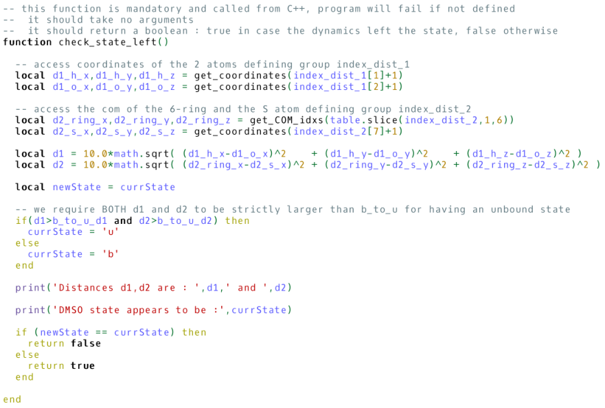
For further increased performance it is possible to use the LuaJIT implementation [68] where the Lua code is compiled to machine code during parsing: this allows performance close to what would be obtained by defining the states based on compiled code
Finally, the Lua layer can act
as an intermediate proxy between the C++ Gen. ParRep code and
any other external library, providing the possibility to define states and observables using external software pieces:
one can for example imagine to use tools such as Colvars [44] or PLUMED [45], providing access to an
extensive ready to use collection of collective variables definitions.
3.4 On the choice of and
As previously mentioned in subsection 2.4 it is not necessary to check at each integration of if (parallel step) or (F-V step) as one expects that the exit time is much larger than .
And likewise, while it is important to regularly gather the value of the G-R observables in order to obtain convergence of Equation (3), it is expected that they will not differ that much between time and : hence it is interesting to choose .
While the values should be fine tuned for each system, based on our experience we ended up with the following rule of thumb: one can take to be to times the value of , and to be to times . This should be adjusted depending on: (i) the amount of calculations involved in the process of defining the state and the G-R observables in the input script, and (ii) the size of the system; for a large solvated protein, if the states and observables only involve distance measures on a few atoms, then the time required for performing the dynamics will be comparatively much larger and relatively small values of and can be selected; however, if it involves tracking the length of several dozens of hydrogen distances, or counting native contacts, a wise approach would be to choose and .
Furthermore, it should be emphasized that while Equation (5) is mathematically valid for any
values of
(in the sense that it indeed samples the exit time of the sub-sampled Markov chain ),
if is taken too large, one may miss an exit event if the process re-enters the same
state during the time interval ;
however one may argue that such cases may denote a poor definition of
the states, and that for states exhibiting strong metastability this should not be an issue.
4 Results and discussion
Now that both the algorithm and the software implementation of the Generalized ParRep (in the following denoted as “Gen. ParRep ”) have been extensively discussed, let us consider two applications: the first validates the implementation and consists in a study of the conformational equilibrium of alanine dipeptide (subsection 4.1), while the second investigates the dissociation of the FKBP–DMSO protein–ligand complex (subsection 4.2).
In the following, when reporting estimated values of the average exit time from a metastable state we will consider the sample average over samples as
Furthermore the confidence interval for those (close to) exponentially distributed samples is:
where is the value of the quantile function of the distribution with degrees of freedom at level ; in the following we chose and therefore report the confidence interval.
4.1 Conformational equilibrium of the alanine dipeptide
The blocked alanine dipeptide (Ac-Ala-N-H-Me) has been used as a validation system for computational studies of conformational equilibria, and energy landscape reconstruction and analysis [69, 70, 71, 72, 73, 74, 75, 76]. The dipeptide contains several notable structural features, including the two dihedral angles, NH- and CO-groups capable of H-bond formation, and a methyl group attached to the atom. One suitable way to visualize the conformations and the transitions between them is to draw an energy surface as a Ramachandran plot [77]: when studied in vacuo the following two metastable states are clearly identified: (i) for , and (ii) for .
In the following we estimate the mean first passage time between the two metastable states, using the
Gen. ParRep algorithm;
accuracy of the method is compared to one long serial Langevin dynamics, as the low
complexity of this system allows direct numerical simulation of numerous transition events;
finally the influence of some of the Gen. ParRep parameters is also evaluated.
4.1.1 MD setup
The initial configuration of the dipeptide is , i.e. within the most
populated area of the state (see the yellow mark on Figure 3 together with a
representation of the corresponding conformation). The OpenMM system was configured as follows:
the CHARMM 22 all-atoms for proteins and
lipids force-field including CMAP corrections [78, 79] was used;
dynamics was performed using a Langevin integrator (time-step of , friction of ), thermostated at a temperature of ;
the non-bonded interactions were evaluated using a non-periodic cutoff scheme up to a distance of ;
and bonds involving hydrogens are constrained to a value of of their original distance.
4.1.2 Gen. ParRep setup
The procedure for defining the states may have to be adapted for each force-field and in the following we assume the use of the aforementioned CHARMM22 force-field. Figure 3 is a Ramachandran plot based free energy surface built from preliminary serial Langevin MD simulation: it illustrates how the ParRep states were a priori defined.
One can see that in the upper left quarter of the plot two close stable conformations indeed coexist, separated by a low energetic barrier of to kcal/mol, which is comparable to the product : hence it was decided to combine those two minima together, as they do not constitute alone a valid metastable target for applying the ParRep method (Refs. [70, 74, 76] indeed suggest that the transition between those two wells is of , and , respectively). Therefore the conformational equilibrium of the dipeptide is modeled using a two states definition:
- 1.
- 2.
The ParRep state consists in the set of all configurations not falling within the red rectangle: it is therefore the complement of the state .
Therefore this setup corresponds to a two states partition of the configuration space projected onto a Ramachandran plot.

Concerning the Fleming-Viot procedure, four Gelman-Rubin observables are considered for tracking the convergence
to the QSD: the total potential energy , the kinetic energy , and the value of
the and dihedral angles acting here as collective variables.
The tolerance criterion is fixed per simulation to a given value which is the same for
each observable (the influence of is investigated below for a range of values).
The value of (accumulation of observables) was set to (i.e. ) as the
observables are not computationally expansive to calculate, and the test
is performed at (i.e. ) during the Convergence step, but at during the
Parallel
dynamics step, which corresponds to , in order to maximize the CPU time spent in the Langevin dynamics.
4.1.3 Discussion
In the following the distribution of the Gen. ParRep sampled values are compared to results obtained when performing a long reference dynamics (denoted as reference MD in the following), consisting in a Langevin dynamics simulation of a total length of . As a result, events were sampled, and is obtained, while the confidence interval is (see Table 1 for a summary); in Ref. [74] the authors estimate to be of (no provided error estimate), in agreement with this value.
First, the possibility to obtain an accurate estimate of by generating a relatively small number of samples is investigated: the number of Gen. ParRep replicas was set to , and the number of samples of generated was for respective tolerance levels of (red, green and blue solid lines; less samples were collected for because of the higher computational effort required for lower tolerance values).
The convergence to the MD reference (black lines) can be visualized on Figure 4 where (solid lines) and the corresponding confidence interval (dashed lines) are given for the three ParRep simulations, when considering only the subset of the first sampled values; the red line () quickly converges to the same distribution than the MD reference, while higher values of appear to converge to a different distribution underestimating (see also numerical values in Table 1): this suggests that convergence to the QSD is only obtained for a value of when studying the transition.
Now that a value of appears to be accurate enough, one can collect more samples in order
to verify that the distribution of the exit times converges to the one obtained with the reference MD simulation.
In Figure 5, the distribution of samples generated for a level of and using
is illustrated: this was done by building an empirical complementary cumulative distribution function
(in the following referred to as ) using the samples, and
it provides an estimate of the probability that is higher than a given value (i.e. ), with by
definition ).
One can see from Figure 5 that the Gen. ParRep and MD distributions are in really good agreement for , where a quasi linear
function (i.e. exponential law) is observed
(we ignore the area for , i.e. the low
probability tail of
the distribution corresponding to large values of , where the MD simulation lacks samples for performing a meaningful
comparison).
This observation is confirmed by looking at Figure 6: the convergence of Gen. ParRep samples to the MD reference is observed, both for the mean value and the confidence interval, for increasing values of
.
4.1.4 Distribution of the F-V estimated value
One last interesting quantity to collect is the time necessary for the convergence of the observables defined by Equation (4) (see subsection 2.4 for more details). Figure 7 provides the histogram distribution of for two of the datasets from Figure 4, together with a Kernel Density Estimate smoothing [80, 81] (dashed lines). For a tolerance of one observes that and appears to follow a normal distribution; for it seems that the distribution is bimodal, with a major mode at and a minor mode at . While it is difficult to argue how the distribution of ideally looks like, one should remember that the is defined as the large funnel on the left () side of Figure 3, and that therefore it encompasses the whole range of the possible values, meaning that will be the slowest observable to converge; it is thus expected that the value of will be large for conservative tolerance levels (), and that depending on how the F-V workers randomly diffused on the surface, its distribution will be broad, possibly multimodal. Hence the dispersion for in Figure 7 appears coherent, while the homogeneous distribution for probably indicates that the F-V workers did not diffuse far enough from their starting point in : they are therefore still distant from what the QSD would be, and this explains why never converged to the result obtained by direct numerical simulation when .
Figure 7 emphasizes one of the main advantages of the Gen. ParRep algorithm versus the original method, i.e. the fact
that is calculated on the fly, and thus adjusted to the initial condition within the state, whereas the original
algorithm required a fixed user defined value
after which it was assumed that the
QSD was reached: indeed, one can see that for (which seems necessary to be sufficiently close to the exact QSD), the
distribution of is
spread over an interval going from to ;
it is therefore obvious that choosing a priori a decorrelation time of would result in a bias as this value appears to be far
below the time it takes to reach the QSD for some initial conditions; and on the contrary choosing a decorrelation time of
would ensure
quasi-convergence to the QSD for most of the initial conditions, but at the cost of an unnecessary long (and then costly) decorrelation
step for some of the initial conditions.
4.1.5 Performance
The last point to discuss concerns the performance of the Gen. ParRep method and particularly the speedup compared with the reference serial Langevin dynamics.
In Table 2 benchmarking data is reported for the simulations from Figure 4; the fifth column reports the calculated effective speedup which is compared to the maximum possible speedup ; the sixth column reports the ratio between the effective speedup (see Table’s caption for methodology) and the maximum possible speedup (hence a value of would indicate a perfect linear speedup).
One can see that for a large tolerance of a value of is obtained, i.e. of the maximum possible value; and for a more conservative tolerance criterion of this falls to i.e. of : this illustrates the cost of an accurate convergence step which, as seen in the previous section, is the key for obtaining accurate results.
Considering the reduced size of the system ( atoms) and the fact that during the F-V procedure the MD engine code is interrupted every
for collecting the value of the G-R observables, this speedup is an impressive result;
although slightly higher values may be obtained by tunning further the values of
and , there is probably little space for optimization for such a small test-case system: therefore a more detailed
performance analysis will be performed in the next subsection for the protein–ligand system.
| WT(s) | (ns) | Speed(ns/day) | Eff. speedup | (Eff./Max.) | |
|---|---|---|---|---|---|
4.2 Dissociation of the FKBP–DMSO protein–ligand system
After validation of the Gen. ParRep algorithm on the alanine dipeptide, we would like to demonstrate its efficiency on a larger protein–ligand system: the aim is to sample the dissociation time between the bound and unbound states of the FKBP–DMSO complex (see Figure 8). The FKBP protein (also known as the FK506 binding protein) have a role in the folding of other proteins containing proline residues [82]; in the human body the FKBP12 protein binds to the tacrolimus molecule (and derivatives), an immunosuppressant drug used to reduce organ rejection after an organ transplant [83]. Because of this important role, both experimental studies [84] and molecular dynamics simulations [85, 86, 87] were performed for evaluating the affinity of the FKBP protein to multiple ligands; these include the DMSO (Dimethyl-sulfoxide), a small molecule with anti-inflammatory, antioxidant and analgesic activities [88], and often used in topical treatments because of its membrane-penetrating ability, which enhances the diffusion of other substances through the skin [89].


4.2.1 MD setup
The initial configuration was taken from the RCSB-PDB entry “1D7H"; the AmberTools17 [63] software suite was used for setting up an implicit solvent input configuration (using the OBC [90] model II): first, parameters for the DMSO ligand were retrieved from the GAFF [91] force-field using the antechamber program; then parameters for the protein are taken from the ff14SB [92] force-field; dynamics was performed using a Langevin integrator (time-step of , friction of ), thermostated at a temperature of ; the non-bonded interactions were evaluated using a non-periodic cutoff scheme up to a distance of ; and bonds involving hydrogens are constrained to a value of of their original distance.
Before running ParRep simulations, the system was equilibrated for ns, with the DMSO’s center of mass being position-constrained
within nm of its original crystallographic position (force constant of 50 kJ/mol/nm2).
4.2.2 Gen. ParRep setup
For defining the ParRep states, we used the following procedure, inspired from Refs. [85, 87]: a closer view at the ligand binding cavity (see Figure 9 (a)) reveals a dense packing with only little available space around the ligand, and one expects that the sulfur and oxygen atoms will interact favorably via non-bonded interactions with the surface of the protein; when observing in details the residues surrounding the DMSO (see Figure 9 (b) corresponding to the RCSB-PDB structure obtained from X-ray diffraction [84]), one can see favorable interaction of the O atom with residue ILE- and of the S atom with residue TRP-.
Hence we used for defining the Gen. ParRep metastable “bound state” (denoted by ) a criteria based on the distances and as illustrated in Figure 9 (b): corresponds to the distance between ligand’s oxygen and the hydrogen amide of residue ILE-; and corresponds to the distance between ligand’s sulfur and the center of mass of the carbons forming the ring of residue TRP-. The DMSO is considered to be in the state when any of or is less than nm, and the “unbound state” (denoted by ) is simply defined as configurations where both distances are larger than nm.


One may wonder whether this distance threshold has a physical meaning: Figure 10 shows a histogram distribution of the two distances and , for a Langevin dynamics, it appears that the threshold of nm corresponds to rarely sampled configurations, far enough from the top of the two distributions ( and nm, respectively), but still closer than the distance range around nm, corresponding to unbound states. This threshold therefore appears to approximately correspond to a boundary between the and states.
Concerning the Fleming-Viot procedure, once again observables were selected in order to track convergence to the QSD:
the two first are the aforementioned distances and ; the third one is the distance between
the center of mass of the DMSO and the center of mass of the protein; the last one is the root mean square velocity of the DMSO ligand.
The levels of were set to the same value for each of the observable, and this value
will be the main Gen. ParRep parameter discussed below.
The value of was set to , and the test
is performed with a period , both during the Convergence step and the Parallel dynamics step.
4.2.3 Discussion
In the following we will compare the Gen. ParRep results to Ref. [87], where the authors performed long explicit water MD simulations using the CHARMM 27 force-field and where a value of is reported.
In Figure 11 the distribution of for tolerance values of is shown (details are available in Table 3): first, a moderate number of transition events () was generated for each level of , and a first estimate of was calculated: as the results for appeared to be far from the results obtained for more stringent tolerances, they were not further considered; then for the three remaining tolerance levels (), extended simulations were performed which permitted to obtain samples of , thus providing estimates of respectively , and with a confidence interval of approximately (see Table 3); the convergence of the corresponding simulations can be observed on Figure 12.
It should first be noted that levels of larger than have to be avoided for this system (and, from our experience, for any application in general) as they will systematically produce biased results: it is indeed not possible to generate initial conditions distributed according to the QSD by using such a loose tolerance criterion, especially when the definition of the state involves a large number of degrees of freedom.
For tolerance levels smaller or equal to 0.05, the confidence intervals mostly overlap, as one can see on Figure 12: for or (respectively the cyan and dark blue lines) the two estimated values of and are almost identical, for (the green line) the estimated value of is , a slightly higher value. A closer look at the upper and lower bounds of the confidence intervals shows a constant overlap — of decreasing width — around , which is the value of for or ( and ), therefore suggesting that, once again, strict tolerance criteria provide the most accurate estimate; this is confirmed by a qualitative (solid vs dashed lines) and quantitative (coefficient ) look at Figure 11, where one can see that the two lowest values of follow the more accurately the quasi-exponential distribution (however, one should remember that the distribution is not expected to be exactly exponential especially for small values of , as exit events of the reference walker happening before the end of the Convergence step are not guaranteed to be exponentially distributed as the QSD was not yet reached).
In the aforementioned Ref. [87] the estimate of is (no confidence interval provided):
this can be considered to be in a reasonable agreement with our value of obtained for and where the
confidence interval is , considering
that the force-field was different, and that the current study uses an implicit solvent while the reference used explicit water molecules.
4.2.4 Performance and convergence to the QSD
Because the FKBP–DMSO system is much more representative of a typical research application than the alanine dipeptide, it is of an utmost interest to provide an accurate estimate of the performances: for this, we provide in Table 4 benchmarking data (following the same methodology established for Table 2): the three datasets correspond to the samples for from Figure 11; the number of replica corresponds to the maximum speedup, while column reports the calculated effective speedup; the ratio given in column gives an idea of the efficiency of the implementation for studying this medium size protein–ligand system.
One can see that the effective speedup is close to (i.e. of the maximum ) for tolerances of and ; for the stricter tolerance level of the speedup falls to (i.e. of the maximum ) which illustrates the computational cost one has to pay for an increased accuracy. Once again the ability to obtain a speedup between and of the maximum possible denotes the parallel efficiency of the Gen. ParRep implementation on a production system, and is an extremely promising achievement towards future studies of larger biochemical systems.
The distribution of is illustrated in Figure 13 for all the considered levels of tolerance: all distributions appear to be multimodal, revealing that multiple sub-states are likely to be found within the surrounding cavity definition of the bound state (this was suggested in earlier studies such as Ref. [86]); for the larger levels of the multimodality is particularly visible with two well defined peaks, resulting in an average falling between the peaks, around ; however for low tolerance such as a broad distribution is observed, and the average goes to .
This emphasizes once again how difficult it would be to fix a priori a value for (as required by the original ParRep implementations), as this value would be inappropriate for some of the initial conditions; the ability of the Gen. ParRep algorithm to automatically determine a value of appropriate for the current initial condition therefore appears to be a major advantage of the method when investigating protein–ligand complexes’ dissociation.
| WT(s) | (ns) | Speed (ns/day) | Eff. speedup | (Eff./Max.) | |
|---|---|---|---|---|---|
5 Conclusion and outlook
In this article, we detailed a new implementation of the Gen. ParRep algorithm, developed with the aim of facilitating
the study of biochemical systems exhibiting strong metastability.
After detailing the methods and the software implementation in Sections 2 and 3,
a validation (Section 4) with two systems of increasing complexity was discussed.
In subsection 4.1, it was shown that the Gen. ParRep method can accurately sample the transition time characterizing
the conformational equilibrium of alanine dipeptide in vacuum: for sufficiently small levels of tolerance (e.g. ), the
estimation converges
to what was obtained from a long reference Langevin dynamics (see Table 1 for a summary, and Figures
3 to 7).
Results also appeared to compare favorably to previously published studies [74].
Finally it was also shown that the implementation of the algorithm proves to be scalable as one can obtain of the maximum
possible speedup (see Table 2).
The second application consisted in the study of the dissociation of the FKBP–DMSO complex (subsection 4.2), a
protein–ligand system of larger size, much more representative of typical metastable problems encountered in computational biology or
chemistry.
The goal was to obtain an accurate estimate of the average time required for observing a dissociation of the complex,
with comparison to previous computational studies [85, 86, 87].
It was shown (see Table 3 and the associated Figures 8 to 13)
that a simple definition of the bound and unbound states based on a two distances threshold can provide an accurate estimate of
, once again when tolerance levels are used: a value of is found
using the Gen. ParRep method,
the value of for appearing to be the most accurate, and this compares relatively well to Ref.
[87]
where a value of was found using a different force-field and an explicit solvent.
The algorithm was also benchmarked for the FKBP–DMSO system (see Table 4), and it was shown
that one can maintain performances up to of the maximum possible speedup on 560 CPU cores,
which definitely makes this new Gen. ParRep ready for production on large scale HPC machines.
From the two studies performed in this article it ought to be remembered that, beyond the accurate definition of the states ,
the choice of the tolerance level is the main parameter
influencing the accuracy of the results:
a value of appears to be the most reasonable choice, confirming previous observations on smaller systems
[43].
Furthermore, the algorithm provides an accurate estimate of the time required for approximating the QSD depending on the initial
condition within the state, and it was shown
(see Figures 7 and 13) that is distributed over a large interval of time: in
such a case the a priori choice of a fixed value decorrelation time approximating (as it was done in the original ParRep
implementations) is non-obvious, and the use of the Gen. ParRep method is justified.
As an outlook, it has to be emphasized that there is still, of course, place for improvement of the software implementation: the authors would like to make the program compatible with other MD engines; tests are currently being performed where replicas are distributed over General-Purpose computing units (GPGPUs) in order to consider applications to larger systems; and preliminary simulations are being performed on a HPC Cloud Computing platform, on which a user could easily use thousands of replicas.
The authors are also currently studying more
advanced biochemical metastable problems, including larger protein–ligand systems in explicit water where the states consist in a set of
disjoint cavities inside a protein.
Acknowledgement
- 1.
This work is supported by the European Research Council under the European Union’s Seventh Framework Program (FP/2007-2013)/ERC Grant Agreement number 614492.
- 2.
The authors acknowledge the “Maison de la Simulation” (and particularly Matthieu Haefele and Julien Derouillat) for helpful discussion and advices concerning the optimization of the software.
- 3.
This work was granted access to the HPC resources of the CINES under the GENCI allocations 2017-AP010710193, 2017-AP010710245 and 2017-A0030710275.
- 4.
FH acknowledges the Institute for Pure and Applied Mathematics (IPAM) at the University of California Los Angeles (UCLA) for participation to the long program “Complex High-Dimensional Energy Landscapes”, its organizers, participants, and particularly members of the “Accelerated dynamics and benchmarking” working group for discussion and remarks on this work.
Bibliography
References
- [1]
A. Hospital, J. R. Goñi, M. Orozco, J. L.
Gelpi, Molecular dynamics
simulations: advances and applications, AABC 8 (2015) 37–47.
doi:10.2147/AABC.S70333.
URL https://doi.org/10.2147/AABC.S70333 - [2]
M. De Vivo, M. Masetti, G. Bottegoni, A. Cavalli,
Role of Molecular
Dynamics and Related Methods in Drug Discovery, J. Med. Chem. 59 (9) (2016)
4035–4061.
doi:10.1021/acs.jmedchem.5b01684.
URL https://doi.org/10.1021/acs.jmedchem.5b01684 - [3]
V. Lounnas, T. Ritschel, J. Kelder, R. McGuire, R. P. Bywater, N. Foloppe,
CURRENT
PROGRESS IN STRUCTURE-BASED RATIONAL DRUG DESIGN MARKS A
NEW MINDSET IN DRUG DISCOVERY, Computational and Structural
Biotechnology Journal 5 (6) (2013) e201302011.
doi:10.5936/csbj.201302011.
URL http://www.sciencedirect.com/science/article/pii/S2001037014600398 - [4] G. Sliwoski, S. Kothiwale, J. Meiler, E. W. Lowe, Computational methods in drug discovery, Pharmacol. Rev. 66 (1) (2014) 334–395. doi:10.1124/pr.112.007336.
- [5]
H. I. Ingólfsson, C. A. Lopez, J. J.
Uusitalo, D. H. de Jong, S. M. Gopal, X. Periole, S. J. Marrink,
The power of coarse graining in
biomolecular simulations, WIREs. Comput. Mol. Sci. 4 (3) (2014) 225–248.
doi:10.1002/wcms.1169.
URL https://doi.org/10.1002/wcms.1169 - [6]
S. Kmiecik, D. Gront, M. Kolinski, L. Wieteska, A. E. Dawid, A. Kolinski,
Coarse-Grained Protein
Models and Their Applications, Chem. Rev. 116 (14) (2016) 7898–7936.
doi:10.1021/acs.chemrev.6b00163.
URL https://doi.org/10.1021/acs.chemrev.6b00163 - [7]
B. Kuhn, P. Mohr, M. Stahl,
Intramolecular Hydrogen Bonding in
Medicinal Chemistry, J. Med. Chem. 53 (6) (2010) 2601–2611.
doi:10.1021/jm100087s.
URL https://doi.org/10.1021/jm100087s - [8]
C. Bissantz, B. Kuhn, M. Stahl, A
Medicinal Chemist’s Guide to Molecular Interactions, J. Med. Chem.
53 (14) (2010) 5061–5084.
doi:10.1021/jm100112j.
URL https://doi.org/10.1021/jm100112j - [9]
H. Jónsson, G. Mills, K. W. Jacobsen,
Nudged
elastic band method for finding minimum energy paths of transitions, WORLD
SCIENTIFIC, 2011, pp. 385–404.
doi:10.1142/9789812839664_0016.
URL http://www.worldscientific.com/doi/abs/10.1142/9789812839664_0016 - [10]
W. E, W. Ren, E. Vanden-Eijnden,
String method for the
study of rare events, Phys. Rev. B 66 (5) (2002) 052301.
doi:10.1103/PhysRevB.66.052301.
URL https://doi.org/10.1103/PhysRevB.66.052301 - [11]
R. Zhao, J. Shen, R. D. Skeel,
Maximum Flux Transition Paths of
Conformational Change, J. Chem. Theory Comput. 6 (8) (2010) 2411–2423.
doi:10.1021/ct900689m.
URL https://doi.org/10.1021/ct900689m - [12] G. A. Huber, S. Kim, Weighted-ensemble Brownian dynamics simulations for protein association reactions., Biophys. J. 70 (1) (1996) 97. doi:10.1016/S0006-3495(96)79552-8.
- [13]
M. C. Zwier, J. L. Adelman, J. W. Kaus, A. J. Pratt, K. F. Wong, N. B. Rego,
E. Suárez, S. Lettieri, D. W. Wang, M. Grabe, D. M. Zuckerman, L. T. Chong,
WESTPA: An interoperable, highly
scalable software package for weighted ensemble simulation and analysis,
Journal of Chemical Theory and Computation 11 (2) (2015) 800–809.
arXiv:https://doi.org/10.1021/ct5010615, doi:10.1021/ct5010615.
URL https://doi.org/10.1021/ct5010615 - [14]
C. Dellago, P. G. Bolhuis, D. Chandler,
On the calculation of reaction rate
constants in the transition path ensemble, J. Chem. Phys. 110 (14) (1999)
6617–6625.
doi:10.1063/1.478569.
URL https://doi.org/10.1063/1.478569 - [15]
F. Cérou, A. Guyader,
Adaptive Multilevel
Splitting for Rare Event Analysis, Stochastic Analysis and Applications
25 (2) (2007) 417–443.
doi:10.1080/07362990601139628.
URL https://doi.org/10.1080/07362990601139628 - [16]
F. Cérou, A. Guyader, T. Lelièvre, D. Pommier,
A multiple replica approach to
simulate reactive trajectories, J. Chem. Phys. 134 (5) (2011) 054108.
doi:10.1063/1.3518708.
URL https://doi.org/10.1063/1.3518708 - [17]
C.-E. Bréhier, T. Lelièvre, M. Rousset,
Analysis of adaptive multilevel
splitting algorithms in an idealized case, ESAIM: PS 19 (2015) 361–394.
doi:10.1051/ps/2014029.
URL http://dx.doi.org/10.1051/ps/2014029 - [18]
I. Teo, C. G. Mayne, K. Schulten, T. Lelièvre, Adaptive
Multilevel Splitting Method for Molecular Dynamics Calculation of
Benzamidine-Trypsin Dissociation Time, J. Chem. Theory Comput. 12 (6)
(2016) 2983–2989.
doi:10.1021/acs.jctc.6b00277.
URL https://doi.org/10.1021/acs.jctc.6b00277 - [19]
T. S. van Erp, P. G. Bolhuis,
Elaborating transition
interface sampling methods, J. Comput. Phys. 205 (1) (2005) 157–181.
doi:10.1016/j.jcp.2004.11.003.
URL https://doi.org/10.1016/j.jcp.2004.11.003 - [20]
R. J. Allen, C. Valeriani, P. R. t. Wolde,
Forward flux sampling
for rare event simulations, J. Phys.: Condens. Matter 21 (46) (2009)
463102.
doi:10.1088/0953-8984/21/46/463102.
URL https://doi.org/10.1088/0953-8984/21/46/463102 - [21]
A. K. Faradjian, R. Elber, Computing
time scales from reaction coordinates by milestoning, J. Chem. Phys.
120 (23) (2004) 10880–10889.
doi:10.1063/1.1738640.
URL https://doi.org/10.1063/1.1738640 - [22]
L. Maragliano, E. Vanden-Eijnden, B. Roux,
Free Energy and Kinetics of
Conformational Transitions from Voronoi Tessellated Milestoning with
Restraining Potentials, J. Chem. Theory Comput. 5 (10) (2009) 2589–2594.
doi:10.1021/ct900279z.
URL https://doi.org/10.1021/ct900279z - [23]
C. Schütte, F. Noé, J. Lu, M. Sarich, E. Vanden-Eijnden,
Markov state models based on
milestoning, J. Chem. Phys. 134 (20) (2011) 204105.
doi:10.1063/1.3590108.
URL https://doi.org/10.1063/1.3590108 - [24]
J. M. Bello-Rivas, R. Elber,
Simulations of thermodynamics and
kinetics on rough energy landscapes with milestoning, J. Comput. Chem.
37 (6) (2016) 602–613.
doi:10.1002/jcc.24039.
URL https://doi.org/10.1002/jcc.24039 - [25]
D. Aristoff, J. M. Bello-Rivas, R. Elber,
A Mathematical Framework for Exact
Milestoning, Multiscale Modeling & Simulationdoi:10.1137/15M102157X.
URL https://doi.org/10.1137/15M102157X - [26] G. Grazioli, I. Andricioaei, Advances in milestoning. I. Enhanced sampling via wind-assisted reweighted milestoning (WARM), J. Chem. Phys. 149 (8) (2018) 084103. doi:10.1063/1.5029954.
- [27] G. Grazioli, I. Andricioaei, Advances in milestoning. II. Calculating time-correlation functions from milestoning using stochastic path integrals, J. Chem. Phys. 149 (8) (2018) 084104. doi:10.1063/1.5037482.
- [28]
A. F. Voter, M. R. Sørensen,
Accelerating Atomistic
Simulations of Defect Dynamics: Hyperdynamics, Parallel Replica Dynamics, and
Temperature-Accelerated Dynamics, MRS Online Proceedings Library Archive
538.
doi:10.1557/PROC-538-427.
URL https://doi.org/10.1557/PROC-538-427 - [29]
D. Perez, B. P. Uberuaga, Y. Shim, J. G. Amar, A. F. Voter,
Chapter
4 accelerated molecular dynamics methods: Introduction and recent
developments, in: R. A. Wheeler (Ed.), Annual Reports in Computational
Chemistry, Vol. 5, Elsevier, 2009, pp. 79 – 98.
doi:https://doi.org/10.1016/S1574-1400(09)00504-0.
URL http://www.sciencedirect.com/science/article/pii/S1574140009005040 - [30]
T. Lelièvre,
Accelerated dynamics:
Mathematical foundations and algorithmic improvements, Eur. Phys. J. Spec.
Top. 224 (12) (2015) 2429–2444.
doi:10.1140/epjst/e2015-02420-1.
URL https://doi.org/10.1140/epjst/e2015-02420-1 - [31] T. Lelièvre, G. Stoltz, Partial differential equations and stochastic methods in molecular dynamics, Acta Numerica 25 (2016) 681–880. doi:10.1017/S0962492916000039.
- [32]
T. Lelièvre,
Mathematical foundations of
Accelerated Molecular Dynamics methods, arXivarXiv:1801.05347.
URL https://arxiv.org/abs/1801.05347 - [33]
A. F. Voter,
Parallel replica
method for dynamics of infrequent events, Phys. Rev. B 57 (1998)
R13985–R13988.
doi:10.1103/PhysRevB.57.R13985.
URL https://link.aps.org/doi/10.1103/PhysRevB.57.R13985 - [34]
O. Kum, B. M. Dickson, S. J. Stuart, B. P. Uberuaga, A. F. Voter,
Parallel replica dynamics with a
heterogeneous distribution of barriers: Application to n-hexadecane
pyrolysis, J. Chem. Phys. 121 (20) (2004) 9808–9819.
doi:10.1063/1.1807823.
URL https://doi.org/10.1063/1.1807823 - [35]
D. Perez, E. D. Cubuk, A. Waterland, E. Kaxiras, A. F. Voter,
Long-Time Dynamics through
Parallel Trajectory Splicing, J. Chem. Theory Comput. 12 (1) (2016) 18–28.
doi:10.1021/acs.jctc.5b00916.
URL https://doi.org/10.1021/acs.jctc.5b00916 - [36]
D. Perez, Parsplice, version
1, version 00 (1 2017).
URL https://www.osti.gov//servlets/purl/1338199 - [37]
A. F. Voter, A method for accelerating
the molecular dynamics simulation of infrequent events, J. Chem. Phys.
106 (11) (1997) 4665–4677.
doi:10.1063/1.473503.
URL https://doi.org/10.1063/1.473503 - [38]
A. F. Voter, Hyperdynamics:
Accelerated Molecular Dynamics of Infrequent Events, Phys. Rev. Lett.
78 (20) (1997) 3908–3911.
doi:10.1103/PhysRevLett.78.3908.
URL https://doi.org/10.1103/PhysRevLett.78.3908 - [39]
M. R. So/rensen, A. F. Voter,
Temperature-accelerated dynamics for
simulation of infrequent events, J. Chem. Phys. 112 (21) (2000) 9599–9606.
doi:10.1063/1.481576.
URL https://doi.org/10.1063/1.481576 - [40]
C. L. Bris, T. Lelièvre, M. Luskin, D. Perez,
A mathematical formalization
of the parallel replica dynamics, Monte Carlo Methods and Applications
18 (2) (2012) 119–146, arXiv: 1105.4636.
doi:10.1515/mcma-2012-0003.
URL https://doi.org/10.1515/mcma-2012-0003 - [41]
P. A. Ferrari, H. Kesten, S. Martinez, P. Picco,
Existence of quasi-stationary
distributions. a renewal dynamical approach, The Annals of Probability
23 (2) (1995) 501–521.
URL http://www.jstor.org/stable/2244994 - [42]
E. van Doorn, P. Pollett,
Quasi-stationary
distributions, no. 1945 in Memorandum / Department of Applied Mathematics,
University of Twente, Department of Applied Mathematics, 2011.
URL https://research.utwente.nl/en/publications/quasi-stationary-distributions - [43]
A. Binder, T. Lelièvre, G. Simpson,
A generalized parallel
replica dynamics, J. Comput. Phys. 284 (2015) 595–616, arXiv: 1404.6191.
doi:10.1016/j.jcp.2015.01.002.
URL https://doi.org/10.1016/j.jcp.2015.01.002 - [44] G. Fiorin, M. L. Klein, J. Hénin, Using collective variables to drive molecular dynamics simulations, Molecular Physics 111 (22-23, SI) (2013) 3345–3362. doi:10.1080/00268976.2013.813594.
- [45]
G. A. Tribello, M. Bonomi, D. Branduardi, C. Camilloni, G. Bussi,
Plumed
2: New feathers for an old bird, Computer Physics Communications 185 (2)
(2014) 604 – 613.
doi:https://doi.org/10.1016/j.cpc.2013.09.018.
URL http://www.sciencedirect.com/science/article/pii/S0010465513003196 - [46]
W. H. FLEMING, M. VIOT, Some
measure-valued markov processes in population genetics theory, Indiana
University Mathematics Journal 28 (5) (1979) 817–843.
URL http://www.jstor.org/stable/24892583 - [47] A. Asselah, P. A. Ferrari, P. Groisman, Quasistationary distributions and fleming-viot processes in finite spaces, Journal of Applied Probability 48 (2) (2011) 322–332. doi:10.1239/jap/1308662630.
- [48]
A. Gelman, D. B. Rubin, Inference
from iterative simulation using multiple sequences, Statistical Science
7 (4) (1992) 457–472.
URL http://www.jstor.org/stable/2246093 - [49]
S. P. Brooks, A. Gelman,
General
methods for monitoring convergence of iterative simulations, Journal of
Computational and Graphical Statistics 7 (4) (1998) 434–455.
doi:10.1080/10618600.1998.10474787.
URL http://www.tandfonline.com/doi/abs/10.1080/10618600.1998.10474787 - [50]
D. Aristoff, T. Lelièvre, G. Simpson,
The Parallel Replica Method for
Simulating Long Trajectories of Markov Chains, Appl. Math. Res. eXpress
2014 (2) (2014) 332–352.
doi:10.1093/amrx/abu005.
URL https://doi.org/10.1093/amrx/abu005 - [51] Mpi: A message-passing interface standard, Tech. rep., The MPI forum, Knoxville, TN, USA (1994).
- [52] E. Gabriel, G. E. Fagg, G. Bosilca, T. Angskun, J. J. Dongarra, J. M. Squyres, V. Sahay, P. Kambadur, B. Barrett, A. Lumsdaine, R. H. Castain, D. J. Daniel, R. L. Graham, T. S. Woodall, Open MPI: Goals, concept, and design of a next generation MPI implementation, in: Proceedings, 11th European PVM/MPI Users’ Group Meeting, Budapest, Hungary, 2004, pp. 97–104.
- [53]
W. Gropp, Mpich2: A new
start for mpi implementations, in: Proceedings of the 9th European PVM/MPI
Users’ Group Meeting on Recent Advances in Parallel Virtual Machine and
Message Passing Interface, Springer-Verlag, London, UK, UK, 2002, p. 7.
URL http://dl.acm.org/citation.cfm?id=648139.749473 - [54]
T. Darden, D. York, L. Pedersen,
Particle mesh Ewald: An
Nlog(N) method for Ewald sums in large systems, J. Chem. Phys.
98 (12) (1993) 10089–10092.
doi:10.1063/1.464397.
URL https://doi.org/10.1063/1.464397 - [55]
F. S. Lee, A. Warshel, A local
reaction field method for fast evaluation of long-range electrostatic
interactions in molecular simulations, J. Chem. Phys. 97 (5) (1992)
3100–3107.
doi:10.1063/1.462997.
URL https://doi.org/10.1063/1.462997 - [56]
I. G. Tironi, R. Sperb, P. E. Smith, W. F. van Gunsteren,
A generalized reaction field method
for molecular dynamics simulations, J. Chem. Phys. 102 (13) (1995)
5451–5459.
doi:10.1063/1.469273.
URL https://doi.org/10.1063/1.469273 - [57]
W. Mattson, B. M. Rice,
Near-neighbor
calculations using a modified cell-linked list method, Comput. Phys.
Commun. 119 (2) (1999) 135–148.
doi:10.1016/S0010-4655(98)00203-3.
URL https://doi.org/10.1016/S0010-4655(98)00203-3 - [58]
Z. Yao, J.-S. Wang, G.-R. Liu, M. Cheng,
Improved neighbor list
algorithm in molecular simulations using cell decomposition and data sorting
method, Comput. Phys. Commun. 161 (1) (2004) 27–35.
doi:10.1016/j.cpc.2004.04.004.
URL https://doi.org/10.1016/j.cpc.2004.04.004 - [59]
T. N. Heinz, P. H. Hünenberger,
A fast pairlist-construction
algorithm for molecular simulations under periodic boundary conditions, J.
Comput. Chem. 25 (12) (2004) 1474–1486.
doi:10.1002/jcc.20071.
URL https://doi.org/10.1002/jcc.20071 - [60]
P. Gonnet, A simple algorithm to
accelerate the computation of non-bonded interactions in cell-based molecular
dynamics simulations, J. Comput. Chem. 28 (2) (2007) 570–573.
doi:10.1002/jcc.20563.
URL https://doi.org/10.1002/jcc.20563 - [61]
P. Eastman, J. Swails, J. D. Chodera, R. T. McGibbon, Y. Zhao, K. A. Beauchamp,
L.-P. Wang, A. C. Simmonett, M. P. Harrigan, C. D. Stern, R. P. Wiewiora,
B. R. Brooks, V. S. Pande,
Openmm 7: Rapid
development of high performance algorithms for molecular dynamics, PLOS
Computational Biology 13 (7) (2017) 1–17.
doi:10.1371/journal.pcbi.1005659.
URL https://doi.org/10.1371/journal.pcbi.1005659 - [62]
B. R. Brooks, I. C. L. Brooks, A. D. MacKerell, Jr., L. Nilsson, R. J.
Petrella, B. Roux, Y. Won, G. Archontis, C. Bartels, S. Boresch, A. Caflisch,
L. Caves, Q. Cui, A. R. Dinner, M. Feig, S. Fischer, J. Gao, M. Hodoscek,
W. Im, K. Kuczera, T. Lazaridis, J. Ma, V. Ovchinnikov, E. Paci, R. W.
Pastor, C. B. Post, J. Z. Pu, M. Schaefer, B. Tidor, R. M. Venable, H. L.
Woodcock, X. Wu, W. Yang, D. M. York, M. Karplus,
CHARMM: The Biomolecular Simulation
Program, J. Comput. Chem. 30 (10) (2009) 1545–1614.
doi:10.1002/jcc.21287.
URL https://doi.org/10.1002/jcc.21287 - [63]
D. A. Case, D. S. Cerutti, T. E. Cheatham, T. A. Darden, R. E. Duke, T. J.
Giese, H. Gohlke, A. W. Goetz, D. Greene, N. Homeyer, S. Izadi, A. Kovalenko,
T. S. Lee, S. LeGrand, P. Li, C. Lin, J. Liu, T. Luchko, R. Luo,
D. Mermelstein, K. M. Merz, G. Monard, H. Nguyen, I. Omelyan, A. Onufriev,
F. Pan, R. Qi, D. R. Roe, A. Roitberg, C. Sagui, C. L. Simmerling, W. M.
Botello-Smith, J. Swails, R. C. Walker, J. Wang, R. M. Wolf, X. Wu, L. Xiao,
D. M. York, P. A. Kollman, Amber16 and
ambertools17, Software, http://ambermd.org/ (2017).
URL http://ambermd.org/ - [64]
M. J. Abraham, T. Murtola, R. Schulz, S. Páll, J. C. Smith, B. Hess, E. Lindahl,
GROMACS: High performance
molecular simulations through multi-level parallelism from laptops to
supercomputers, SoftwareX 1-2 (2015) 19–25.
doi:10.1016/j.softx.2015.06.001.
URL https://doi.org/10.1016/j.softx.2015.06.001 - [65]
J. C. Phillips, R. Braun, W. Wang, J. Gumbart, E. Tajkhorshid, E. Villa,
C. Chipot, R. D. Skeel, L. Kalé,
K. Schulten, Scalable molecular
dynamics with NAMD, J. Comput. Chem. 26 (16) (2005) 1781–1802.
doi:10.1002/jcc.20289.
URL https://doi.org/10.1002/jcc.20289 - [66]
R. Ierusalimschy, L. H. de Figueiredo, W. C. Filho,
Lua—an
extensible extension language, Software: Practice and Experience 26 (6)
(1996) 635–652.
doi:10.1002/(SICI)1097-024X(199606)26:6<635::AID-SPE26>3.0.CO;2-P.
URL http://dx.doi.org/10.1002/(SICI)1097-024X(199606)26:6<635::AID-SPE26>3.0.CO;2-P - [67]
ThePhD, sol2: a c++ - lua api
wrapper, Software, version 2.17.5, https://github.com/ThePhD/sol2 (June
2017).
URL https://github.com/ThePhD/sol2 - [68]
M. Pall, Luajit, a Just-In-Time Compiler (JIT) for
the Lua programming language, Software, version 2.0.5, http://luajit.org/
(May 2017).
URL http://luajit.org/ - [69]
J. Apostolakis, P. Ferrara, A. Caflisch,
Calculation of conformational
transitions and barriers in solvated systems: Application to the alanine
dipeptide in water, J. Chem. Phys. 110 (4) (1999) 2099–2108.
doi:10.1063/1.477819.
URL https://doi.org/10.1063/1.477819 - [70]
H. M. Chun, C. E. Padilla, D. N. Chin, M. Watanabe, V. I. Karlov, H. E. Alper,
K. Soosaar, K. B. Blair, O. M. Becker, L. S. D. Caves, R. Nagle, D. N. Haney,
B. L. Farmer,
MBO(N)D:
A multibody method for long-time molecular dynamics simulations, J.
Comput. Chem. 21 (3) (2000) 159–184.
doi:10.1002/(SICI)1096-987X(200002)21:33.0.CO;2-J.
URL https://doi.org/10.1002/(SICI)1096-987X(200002)21:33.0.CO;2-J - [71]
W. C. Swope, J. W. Pitera, F. Suits, M. Pitman, M. Eleftheriou, B. G. Fitch,
R. S. Germain, A. Rayshubski, T. J. C. Ward, Y. Zhestkov, R. Zhou,
Describing Protein Folding Kinetics
by Molecular Dynamics Simulations. 2. Example Applications to Alanine
Dipeptide and a -Hairpin Peptide, J. Phys. Chem. B 108 (21) (2004)
6582–6594.
doi:10.1021/jp037422q.
URL https://doi.org/10.1021/jp037422q - [72]
W. Ren, E. Vanden-Eijnden, P. Maragakis, W. E,
Transition pathways in complex
systems: Application of the finite-temperature string method to the alanine
dipeptide, J. Chem. Phys. 123 (13) (2005) 134109.
doi:10.1063/1.2013256.
URL https://doi.org/10.1063/1.2013256 - [73]
H. Jang, T. B. Woolf, Multiple
pathways in conformational transitions of the alanine dipeptide: An
application of dynamic importance sampling, J. Comput. Chem. 27 (11) (2006)
1136–1141.
doi:10.1002/jcc.20444.
URL https://doi.org/10.1002/jcc.20444 - [74]
B. Strodel, D. J. Wales,
Free energy surfaces
from an extended harmonic superposition approach and kinetics for alanine
dipeptide, Chem. Phys. Lett. 466 (4) (2008) 105–115.
doi:10.1016/j.cplett.2008.10.085.
URL https://doi.org/10.1016/j.cplett.2008.10.085 - [75]
P. T. Vedell, Z. Wu,
The
solution of the boundary-value problems for the simulation of transition of
protein conformation, International Journal of Numerical Analysis and
Modeling 10 (4) (2013) 920–942.
URL http://www.math.ualberta.ca/ijnam/Volume-10-2013/No-4-13/2013-04-11.pdf - [76]
C. Velez-Vega, E. E. Borrero, F. A. Escobedo,
Kinetics and reaction coordinate
for the isomerization of alanine dipeptide by a forward flux sampling
protocol, J. Chem. Phys. 130 (22) (2009) 225101.
doi:10.1063/1.3147465.
URL https://doi.org/10.1063/1.3147465 - [77]
G. N. Ramachandran, C. Ramakrishnan, V. Sasisekharan,
Stereochemistry of
polypeptide chain configurations, J. Mol. Biol. 7 (1) (1963) 95–99.
doi:10.1016/S0022-2836(63)80023-6.
URL https://doi.org/10.1016/S0022-2836(63)80023-6 - [78]
A. D. MacKerell, D. Bashford, M. Bellott, R. L. Dunbrack, J. D. Evanseck, M. J.
Field, S. Fischer, J. Gao, H. Guo, S. Ha, D. Joseph-McCarthy, L. Kuchnir,
K. Kuczera, F. T. K. Lau, C. Mattos, S. Michnick, T. Ngo, D. T. Nguyen,
B. Prodhom, W. E. Reiher, B. Roux, M. Schlenkrich, J. C. Smith, R. Stote,
J. Straub, M. Watanabe, J. Wiórkiewicz-Kuczera, D. Yin, M. Karplus,
All-atom empirical potential for
molecular modeling and dynamics studies of proteins, The Journal of Physical
Chemistry B 102 (18) (1998) 3586–3616, pMID: 24889800.
doi:10.1021/jp973084f.
URL http://dx.doi.org/10.1021/jp973084f - [79]
A. D. Mackerell, M. Feig, C. L. Brooks,
Extending the treatment of
backbone energetics in protein force fields: Limitations of gas-phase quantum
mechanics in reproducing protein conformational distributions in molecular
dynamics simulations, Journal of Computational Chemistry 25 (11) (2004)
1400–1415.
doi:10.1002/jcc.20065.
URL http://dx.doi.org/10.1002/jcc.20065 - [80]
M. Rosenblatt, Remarks on Some
Nonparametric Estimates of a Density Function, Annals of Mathematical
Statistics 27 (3) (1956) 832–837.
doi:10.1214/aoms/1177728190.
URL https://doi.org/10.1214/aoms/1177728190 - [81]
E. Parzen, On Estimation of a
Probability Density Function and Mode, Annals of Mathematical Statistics
33 (3) (1962) 1065–1076.
doi:10.1214/aoms/1177704472.
URL https://doi.org/10.1214/aoms/1177704472 - [82]
J. J. Siekierka, S. H. Y. Hung, M. Poe, C. S. Lin, N. H. Sigal,
A cytosolic binding protein for the
immunosuppressant FK506 has peptidyl-prolyl isomerase activity but is
distinct from cyclophilin, Nature 341 (6244) (1989) 755.
doi:10.1038/341755a0.
URL https://doi.org/10.1038/341755a0 - [83]
T. Wang, P. Donahoe, A. Zervos,
Specific interaction of type
I receptors of the TGF-beta family with the immunophilin FKBP-12, Science
265 (5172) (1994) 674–676.
doi:10.1126/science.7518616.
URL https://doi.org/10.1126/science.7518616 - [84]
P. Burkhard, P. Taylor, M. D. Walkinshaw,
X-ray
structures of small ligand-FKBP complexes provide an estimate for hydrophobic
interaction energies1 1Edited by R. Huber, J. Mol. Biol. 295 (4) (2000)
953–962.
doi:10.1006/jmbi.1999.3411.
URL http://www.sciencedirect.com/science/article/pii/S0022283699934113 - [85]
D. Huang, A. Caflisch, The
Free Energy Landscape of Small Molecule Unbinding, PLoS Comput. Biol. 7 (2)
(2011) e1002002.
doi:10.1371/journal.pcbi.1002002.
URL https://doi.org/10.1371/journal.pcbi.1002002 - [86]
D. Huang, A. Caflisch, Small
Molecule Binding to Proteins: Affinity and Binding/Unbinding Dynamics from
Atomistic Simulations, ChemMedChem 6 (9) (2011) 1578–1580.
doi:10.1002/cmdc.201100237.
URL https://doi.org/10.1002/cmdc.201100237 - [87]
M. Xu, A. Caflisch, P. Hamm,
Protein Structural Memory
Influences Ligand Binding Mode(s) and Unbinding Rates, J. Chem. Theory
Comput. 12 (3) (2016) 1393–1399.
doi:10.1021/acs.jctc.5b01052.
URL https://doi.org/10.1021/acs.jctc.5b01052 - [88]
G. Smith, A. L. Bertone, C. Kaeding, E. J. Simmons, S. Apostoles,
Anti-inflammatory effects
of topically applied dimethyl sulfoxide gel on endotoxin-induced synovitis in
horses, Am. J. Vet. Res. 59 (9) (1998) 1149–1152.
URL https://www.ncbi.nlm.nih.gov/pubmed/9736394 - [89]
Z. Malik, G. Kostenich, L. Roitman, B. Ehrenberg, A. Orenstein,
Topical application of
5-aminolevulinic acid, DMSO and EDTA: protoporphyrin IX accumulation in skin
and tumours of mice, J. Photochem. Photobiol., B 28 (3) (1995) 213–218.
doi:10.1016/1011-1344(95)07117-K.
URL https://doi.org/10.1016/1011-1344(95)07117-K - [90]
A. Onufriev, D. Bashford, D. A. Case,
Exploring protein native states
and large-scale conformational changes with a modified generalized born
model, Proteins: Structure, Function, and Bioinformatics 55 (2) (2004)
383–394.
doi:10.1002/prot.20033.
URL http://dx.doi.org/10.1002/prot.20033 - [91]
J. Wang, R. M. Wolf, J. W. Caldwell, P. A. Kollman, D. A. Case,
Development and testing of a
general amber force field, J. Comput. Chem. 25 (9) (2004) 1157–1174.
doi:10.1002/jcc.20035.
URL https://doi.org/10.1002/jcc.20035 - [92]
J. A. Maier, C. Martinez, K. Kasavajhala, L. Wickstrom, K. E. Hauser,
C. Simmerling, ff14SB:
Improving the Accuracy of Protein Side Chain and Backbone Parameters from
ff99SB, J. Chem. Theory Comput. 11 (8) (2015) 3696–3713.
doi:10.1021/acs.jctc.5b00255.
URL https://doi.org/10.1021/acs.jctc.5b00255