Three-dimensional interstellar dust reddening maps of the Galactic plane
Abstract
We present new three-dimensional (3D) interstellar dust reddening maps of the Galactic plane in three colours, , and . The maps have a spatial angular resolution of 6 arcmin and covers over 7000 deg2 of the Galactic plane for Galactic longitude 0° 360° and latitude °. The maps are constructed from robust parallax estimates from the Gaia Data Release 2 (Gaia DR2) combined with the high-quality optical photometry from the Gaia DR2 and the infrared photometry from the 2MASS and WISE surveys. We estimate the colour excesses, , and , of over 56 million stars with the machine learning algorithm Random Forest regression, using a training data set constructed from the large-scale spectroscopic surveys LAMOST, SEGUE and APOGEE. The results reveal the large-scale dust distribution in the Galactic disk, showing a number of features consistent with the earlier studies. The Galactic dust disk is clearly warped and show complex structures possibly spatially associated with the Sagittarius, Local and Perseus arms. We also provide the empirical extinction coefficients for the Gaia photometry that can be used to convert the colour excesses presented here to the line-of-sight extinction values in the Gaia photometric bands.
Keywords:
ISM: dust, extinction – ISM: structure – Galaxy: structure1 Introduction
The interstellar dust extinction poses a serious challenge for the study of the structure, formation and evolution of our Galaxy, especially for the low Galactic latitude disk regions (Chen et al., 2017b). For any stellar study near the Galactic plane, one needs to correct for the effects of dust extinction and reddening to interpret the observations properly.
Traditional two-dimensional (2D) extinction maps give the total amount of extinction in a given direction integrated along the line-of-sight. Consequently, the value represents an upper limit of the real one for a local disc star in that direction. In the past decades, thanks to a number of large-scale photometric and spectroscopic surveys, such as the Sloan Digital Sky Survey (SDSS; York et al. 2000), the Two Micron All Sky Survey (2MASS; Skrutskie et al. 2006), the LAMOST Experiment for Galactic Understanding and Exploration (LEGUE; Deng et al. 2012; Zhao et al. 2012) and the Pan-STARRS 1 Survey (PS1; Chambers et al. 2016), three-dimensional (3D) extinction maps constructed based on estimates of the distances and extinction values to millions of individual stars have become available.
Based on the 2MASS data, Marshall et al. (2006) present a three-dimensional (3D) extinction model of the inner Galaxy ( 100° and 10°) by comparing the observed colours of giant stars for each line of sight with the synthetic values from the Besançon Galactic model (Robin et al., 2003). Using a similar method, Chen et al. (2013) and Schultheis et al. (2014) present the colour excess maps for several colours toward the Galactic Bulge ( 10° and 10° 5°) based on data from the ESO Public Survey, VISTA Variables in the Via Lactea (VVV; Minniti et al. 2010) and the Galactic Legacy Infrared Mid-Plane Survey Experiment (GLIMPSE; Churchwell et al. 2009). By combining the SDSS optical and the 2MASS near-IR photometry, Berry et al. (2012) simultaneously estimate distances and values of extinction of stars by fitting the observed optical (and IR) spectral energy distributions (SEDs). Analogously, Chen et al. (2014) present a 3D extinction map that covers the entire Xuyi Schmidt Telescope Photometric Survey of the Galactic Anticentre (XSTPS-GAC) survey area of over 6000 deg2 (140° 220°and 40°), based on the XSTPS-GAC optical and the 2MASS and Wide-Field Infrared Survey Explorer (WISE; Wright et al. 2010) IR photometry. Using a hierarchical Bayesian model, Sale et al. (2014) derive a 3D extinction map in the Northern Galactic Plane (30° 215°and 5°) from the optical photometry of the INT/WFC Photometric H Survey (IPHAS; Drew et al. 2005). Green et al. (2015) and Green et al. (2018) apply the Bayesian approach to the PS1 optical and the 2MASS IR photometry to produce 3D maps of dust reddening over three quarters of the sky ( 30°). Hanson et al. (2016) present 3D extinction maps within a few degrees of the Galactic plane (0° 250°and from 4.5°) based on photometry of the PS1 and GLIMPSE surveys. Gontcharov (2017) present a 3D dust reddening map with a radius of 1200 pc around the Sun and within 600 pc of the Galactic midplane based on the colour-magnitude diagram of the 2MASS photometry. Lallement et al. (2014) and Lallement et al. (2018) apply an inversion method to data collected from a variety of catalogues and construct 3D extinction maps of the local interstellar dust. Rezaei Kh. et al. (2017) and Rezaei Kh. et al. (2018) also developed a 3D inversion method, treating the dust density field as a Gaussian process.
Distance is a key parameter to build a 3D extinction map. Most of the works mentioned above derive distances to individual stars based on the photometric parallax relations, with typical uncertainties of about 20 per cent for dwarfs and more for giants (Chen et al., 2014; Green et al., 2014). The second Gaia data release (Gaia DR2, Gaia Collaboration et al. 2016; Gaia Collaboration et al. 2018b) contains parallax estimates for over one billion stars. For stars of magnitudes ranging between 8 and 18 mag, the parallax uncertainties vary between 0.04 and 0.1 mas, corresponding to distance uncertainties better than 20 per cent out to 5 kpc (Lindegren et al., 2018). Based on data published in the Gaia DR2, Bailer-Jones et al. (2018) provide distance estimates of individual stars inferred from procedure that accounts for the non-linearity of the transformation and the asymmetry of the resulting probability distribution. The Gaia DR2 also includes high quality photometry in three bands, , and (Evans et al., 2018). The robust distance estimates and the precise photometry of Gaia DR2 provide us a great opportunity to construct high-quality 3D extinction map of the Galactic disk.
Andrae et al. (2018) have recently estimated values of extinction and colour excess for 88 million stars based on the photometry and parallax of Gaia DR2. However, as they point out, their results, using only three optical bands and parallax, suffer from large uncertainties. There is a significant degeneracy between the intrinsic colours (or effective temperature) and extinction using just optical colours (Bailer-Jones, 2011; Andrae et al., 2018). Berry et al. (2012) show that the degeneracy can be broken (or reduced) by introducing the IR colours. In the current work, we combine the Gaia optical with the 2MASS and WISE IR photometry, and obtain robust estimates of colour excess in several colours for tens of millions of stars in the Galactic disk ( 10°). We adopt the Random Forest regression, a machine learning algorithm, to derive the values of colour excess. Compared to the traditional SED fitting or Bayesian approaches, this machine learning algorithm works much faster to provide results of similar accuracies (see Sect. 5.2). The results are then used to construct 3D colour excess maps of the Galactic disk.
The paper is structured as following. In Section 2, we present the relevant Gaia DR2, 2MASS and WISE data. Section 3 describes the methods used to derive values of colour excess and to construct the 3D colour excess maps. In Section 4, we present our main results which are discussed in Section 5. We summarize in Section 6.
2 Data
Our work is based on broadband photometry from three all-sky surveys, the Gaia, 2MASS and WISE.
The Gaia DR2 (Gaia Collaboration et al., 2018b), released in April 2018, provides high precision positions and broad band photometric measurements for 1.7 billion sources. Amongst them, 1.4 billion sources have and magnitudes and 1.3 billion sources have parallax and proper motion measurements. The band covers the whole optical wavelength range from 330 to 1050 nm. The and magnitudes are derived from the low resolution spectrophotometric measurements integrated over the wavelength ranges 330 - 680 nm and 630 - 1050 nm, respectively. The internal validation of the Gaia DR2 shows that the calibration uncertainties for , and are 2, 5 and 3 mmag, respectively.
To break the degeneracy of effective temperature (or intrinsic colours) and extinction for the individual stars, we combine the Gaia optical photometry with the IR photometry of 2MASS and WISE. The 2MASS survey has three near-IR bands, and , centered at 1.25, 1.65 and 2.16 m, respectively. The 2MASS Point Source Catalog (PSC; Skrutskie et al. 2006) provides photometry for over 500 million objects. The uncertainties of 2MASS photometric measurements are estimated to be smaller than 0.03 mag. The WISE survey has four IR bands, to , centered at 3.4, 4.6, 12 and 22 m, respectively. The AllWISE Source Catalog (Kirkpatrick et al., 2014) provides four band magnitudes and variability statistics for over 747 million objects. For the WISE, we use only the data of band , as the longer wavelength measurements have lower sensitivities and poorer angular resolutions. Including the latter in the analysis do not improve the parameter estimation. The angular resolution of the WISE -band photometry is 6.1′′.
We select stars from the Gaia DR2 with Galactic latitude 10° and then cross-match them with the 2MASS PSC and the AllWISE Source catalogues using the Centre de Donnes astronomiques de Strasbourg (CDS) XMatch Service11 1 http://cdsxmatch.u-strasbg.fr/xmatch. The matching radius is set to 1.5′′. The fraction of multiple matches is less than 0.01 per cent and the matches of the closest positions are adopted. We select sample stars by requiring that the sources must be detected in all Gaia and 2MASS bands, i.e. Gaia , and , and 2MASS , and . We further require that the sources have photometric errors less than 0.08 mag in all six bands and 2MASS quality of ‘AAA’. The cuts lead to a total of 56,431,558 stars in the final catalogue. The Gaia -band magnitude distribution of all the selected stars is illustrated in Fig. 1. Most of the stars have a -band magnitude between 8 and 18 mag. For a given star in the catalogue, its WISE -band magnitude will be adopted only when the photometric error is less than 0.08 mag and no other stars are detected within 6.1′′, the angular resolution of the WISE band in the combined photometric catalogue. As a result, the -band magnitude is only used for just over 73 per cent sources. The -band magnitude distribution of these latter stars is also plotted in Fig. 1.
3 Method


In the SED fitting or Bayesian approach, one uses gridding (Berry et al., 2012; Chen et al., 2014) or the Markov chain Monte Carlo (MCMC) methods (Green et al., 2014; Sale et al., 2014) to sample the parameter space in order to derive the extinction (or colour excess) values of the individual stars. In the current work, we build a model that returns the colour excess values of stars given the data described in Section 2. The model is based on a machine-learning algorithm, the Random Forest regression, one of the most effective machine learning models for predictive analytics. A Random Forest regression is a meta estimator that fits a number of decision trees to various sub-samples of the dataset and uses average values to improve the predictive accuracy while controls over-fitting. We employ the Random Forest regression to estimate the colour excesses, , and of the individual stars. We have also tried other machine learning algorithms, such as the Support Vector Machine and Extra-Tree regressions and found very similar results.
3.1 Training data set
We first create an empirical training set using stars from the spectroscopic surveys. Based on the stellar atmospheric parameters (Teff, log and [Fe/H]) from the spectra, we are able to obtain accurate colour excesses of the individual stars. We collect stars from the LAMOST and SDSS spectroscopic surveys. A star-pair method is adopted to obtain the values of colour excesses of these stars. The star-pair method is straightforward. It is based on the assumption that stars of the same stellar atmospheric parameters have the same intrinsic colours. Thus we can derive the intrinsic colours of a reddened star from its pairs/counterparts of the same atmospheric parameters that suffer from either nil or well-known extinction. In this work, we calculate values of , and for stars from the spectroscopic surveys using the same star-pair algorithm of Yuan et al. (2015). Firstly, a control sample22 2 We note that this control sample is not the training data sample at all. The control sample is only used for the determination of colour excess of stars in the training sample. containing stars with nil or well-known extinction is built. We select stars of the control sample that suffer from very low values of extinction such that their values can be well approximated by the reddening map of Schlegel et al. (1998, SFD). For a given target star in the spectroscopic catalogues, its intrinsic colours, , and , are estimated simultaneously from the corresponding values of the pair stars in the control sample. The values of , and of the target star are then simply calculated from the differences between the observed and intrinsic colours,
The second release of value-added catalogues of the LAMOST Spectroscopic Survey of the Galactic Anticentre (LSS-GAC DR2; Xiang et al. 2017) provides stellar atmospheric parameters deduced from 1.8 million spectra. The catalogues for internal usage include all the observations collected by 2016 June and contains robust stellar parameters estimated from over 5 million spectra (Xiang et al., 2017; Chen et al., 2018). We select stars from the LSS-GAC DR2 with the criteria: LAMOST spectral S/N(4650Å) per pixel 10, ‘objtype’ ‘STAR’, ‘moondis’ 30°, ‘BADFIBER’ 0, ‘SATFIBER’ 0, ‘BRIGHTFIBER’ 0, ‘vr_flag’ 6 and photometric errors err(, , , , ) 0.1 mag. The requirements lead to 3,485,460 stars for the LAMOST sample. Values of , and are calculated for the LAMOST sample using the aforementioned star-pair technique. The control sample for the LAMOST stars, which contains 48,243 stars, is defined by requiring S/N(4650Å) per pixel 50, SFD 0.015 mag and err(, , , , ) 0.03 mag.
We also use data from the SDSS DR14 that provides reliable stellar parameters for 0.4 million stars from the Sloan Extension for Galactic Understanding and Exploration (SEGUE; Yanny et al. 2009) and 0.2 million stars from the Apache Point Observatory Galactic Evolution Experiment (APOGEE; Majewski et al. 2010). Since the LAMOST surveys mainly the outer disc of the Galaxy, thus the SEGUE and APOGEE data sets complement that of LAMOST. To minimize potential systematics between stellar parameters yielded by the different surveys, colour excesses , and are calculated separately for the SEGUE and APOGEE samples, using the same aforementioned star-pair technique. We select stars from the SEGUE and APOGEE catalogues with the criteria: S/N 10, 0, log 0, [Fe/H] or [M/H] and err(, , , , ) 0.1 mag. The requirements yield 116,006 and 142,994 stars for the SEGUE and APOGEE samples, respectively. The SEGUE and APOGEE control samples are defined by requiring S/N 50, SFD 0.015 mag and err(, , , , ) 0.08 mag. The cuts yield 6,386 and 6,579 stars in the SEGUE and APOGEE control samples, respectively.
In Fig. 2 we compare estimates of , and for common stars of the LAMOST and the SEGUE and APOGEE samples. We find no systematics amongst the different samples. For the LAMOST and SEGUE samples, the dispersions of differences are respectively 0.06, 0.03 and 0.008 mag for , and differences. The corresponding values are 0.08, 0.04 and 0.006 mag between the LAMOST and APOGEE samples.
The resulted LAMOST, SEGUE and APOGEE samples are then combined. Abnormal colour excess estimates are excluded by plotting the intrinsic colours, , and , versus (Fig. 3), taking the advantage that the intrinsic colours of stars correlates well with effective temperature. We reject stars that deviate more than 0.2, 0.15 and 0.05 mag from the best-fit , and versus relations, respectively. This leads us to a sample consisting 3,224,373 stars, which is adopted as the final training data set to calculate the colour excesses of stars in the photometric sample by the Random Forest regression. The -band magnitude distribution of the training sample is also plotted in Fig. 1. The magnitudes range between 8 and 19 mag, similar to the photometric sample. In Fig. 4, we show the distribution of these stars in the Galactic coordinates and in the versus plane. The sample covers almost all the Galactic latitudes and about two thirds of the Galactic longitudes. The effective temperatures range between 3000 and 10500 K. The estimated values can be as high as 6 mag, corresponding to 3 mag (based on the extinction coefficients presented in Sect. 5.1). We note that the derived colour excesses for stars in the spectroscopic sample can be smaller than 0 but larger than 0.05 mag, as a result of the photometric errors.
3.2 Colour excesses determinations
The stars in the final spectroscopic sample are randomly divided into two sub-samples, a training sample consisting of 80 per cent of stars and a test sample containing the remaining 20 per cent stars. The training sample is used to generate the Random Forest models, while the test sample is used to validate the generated relations. We build three separate Random Forest models for , and , respectively. In all cases, the input parameters are , , , and . An extra colour will also be used for stars that have data available. We use the scikit-learn package for Python (Pedregosa et al., 2011) to build the models. We test with different parameters to optimize the models. Finally we set the number of trees in the forest to be n_estimators=200, the number of features to consider when looking for the best split to be max_features=‘auto’, the minimum number of samples required to split an internal node to be min_samples_split=2 and the minimum number of samples needed at a leaf node to be min_samples_leaf=1. The 16th and 84th percentiles of the Random Forest ensemble are taken as the uncertainties. Fig. 5 compares the values of , and yielded by the Random Forest models and those given by the star-pair technique for the test sample stars. The Figure shows good agreement in all cases. There is no systematics in the residuals. The standard deviations of the differences are 0.07, 0.04 and 0.005 for , and , respectively, comparable to what expected from the typical uncertainties of colour excess of the spectroscopic sample.
3.3 3D colour excess distribution mapping
For distances of the stars, we adopt the values from Bailer-Jones et al. (2018) who calculate distances of 1.3 billion stars from the Gaia measurements, imposing a prior based on the expected distribution of all stars in the Gaia catalogue. In the current work, we accept the distance estimates only for stars with Gaia parallax uncertainties smaller than 20 per cent. This leads to a sample containing 35,354,103 stars. The -band magnitude distribution of these stars is also shown in Fig. 1. Because of the cut in parallax errors, the number of stars drops dramatically at 18 mag.
To map the 3D dust distribution in the Galactic plane, a procedure similar to that of Green et al. (2014) and Chen et al. (2017a) is adopted. We divide the sample stars into subfields (pixels) of size 6 6 arcmin. For each pixel, we define the reliable depth of our extinction map as the maximum distance of all the individual stars in that pixel. In Fig. 6 we present a map of those depths. The maximum distance is typically 4 kpc, rising up to 6 kpc for regions of the smallest dust extinction. There are some stripe-like features in the map. They are artifacts caused by the scanning nature of the Gaia observations.
For each pixel, the colour excess profile as a function of distance is then derived by fitting the colour excess as a function of distance for the individual stars in that pixel. Here refers to colour excess , or . At a given distance , the colour excess is parameterized by a piecewise linear function,
| (1) |
where is colour excess produced by the local dust grains in the -th distance bin ( is the distance of the bin). is set to be no less than zero to prevent negative reddenings. The length of each distance bin is set as kpc.
Assuming a set of for a given pixel, we are able to model the colour excesses of any star of index in the pixel from Eq. (1). We perform an MCMC analysis to find the best set of of the pixel that maximise the likelihood defined as,
| (2) |
where is index of star in the pixel,
and are respectively the colour excess derived in
Sect. 3.2 and that given by Eq. (1) of the star, is the combined
uncertainty of the derived colour excess () and distance (),
given by ,
is the distance of the star (Lallement et al., 2014; Chen et al., 2017a)),
and is the total number of stars in the pixel. We note that the error
resulting
from the distance error is only an approximation under the
assumption that the dust opacity is constant along the line of sight.
In the current work, the
distance uncertainties are simply adopted as , where
and are respectively the upper and lower bounds of the 68 per cent confidence interval
of the distance estimate from Bailer-Jones et al. (2018).
The median number of stars in a pixel is 45.
About 1000 ( 0.1 pre cent) pixels do not have enough stars ( 3) to
obtain the colour excess profile. We have enlarged those pixels to size of 15 15 arcmin.
The uncertainties of
are computed from 68 per cent probability intervals of
the marginalized probability distribution functions (PDFs) of each
parameter, given by the accepted values after post-burn period in
the MCMC chain. Histogram distribution
of the resulted uncertainties of
is shown in Fig. 7.
4 Dust reddening maps
| Column | Name | Description |
|---|---|---|
| 1 | Galactic longitude (°) of the pixel | |
| 2 | Galactic latitude (°) of the pixel | |
| 3 | Reliable depth (kpc) of the pixel | |
| 4 33 | Integrated as a function of distance ranging from 0.2 to 6 kpc with a step of 0.2 kpc | |
| 34 63 | Errors of | |
| 64 93 | Integrated as a function of distance ranging from 0.2 to 6 kpc with a step of 0.2 kpc | |
| 94 123 | Errors of | |
| 124 153 | Integrated as a function of distance ranging from 0.2 to 6 kpc with a step of 0.2 kpc | |
| 154 183 | Errors of |


Our resulted 3D colour excess maps are available
in electronic form in the online version of this manuscript33
3
Table 1 is also available online via
“http://paperdata.china-vo.org/diskec/cestar/table1.zip”..
Table 1 describes the data format. Each row of the catalogue contains
information of one subfield (pixel): Galactic coordinates and , the reliable depth ,
measured values of the integrated , and and the associated
uncertainties at the individual distance bins. In addition, the colour excesses, , and and
the associated errors of each star in the combined photometric sample are
available upon request by email.
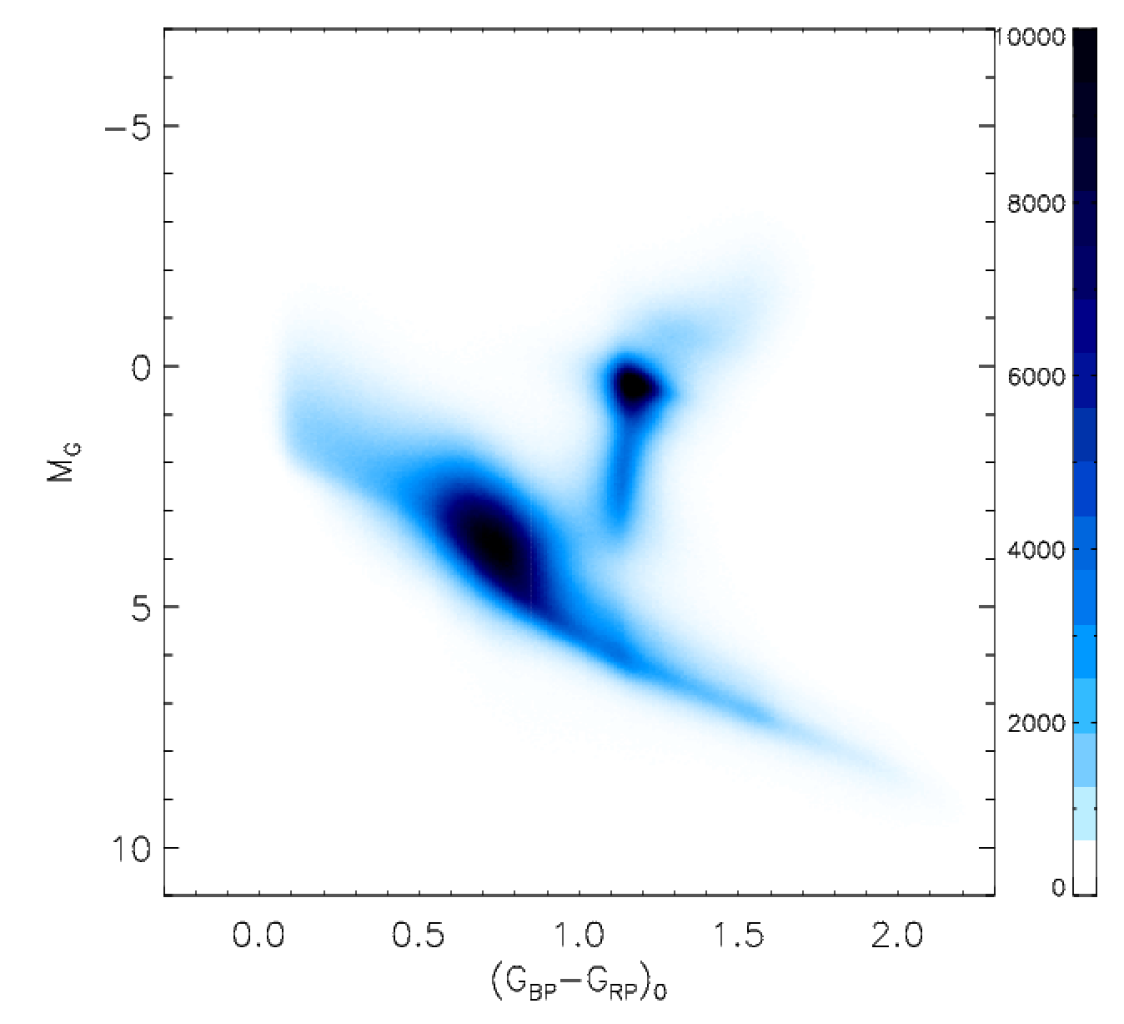
Fig. 8 plots the dust corrected colour and absolute magnitude diagram for
over 35 million stars with Gaia parallax errors smaller than 20 per cent.
Values of absolute magnitude of the individual stars are estimated using the
standard relation, , where is distance estimate from
Bailer-Jones et al. (2018) and the -band line-of-sight extinction. As the Gaia band covers
a wide wavelength range, we calculate from colour excess
and line of sight extinction , as , where
is obtained from
using the near-IR extinction law of Yuan et al. (2013), . So we have
| (3) |
Fig. 8 presents a nice Hertzsprung-Russell diagram (HRD) very similar to the HRD presented in Fig. 5 of Gaia Collaboration et al. (2018a) which is constructed using low-extinction stars. The main sequence is quite sharp, the red clump really a clump and the red giant branch clearly visible. The well-defined HRD presented in Fig. 8 suggests the robustness of colour excess values derived in the current work.
We plot in Fig. 9 2D maps of colour excess in the Galactic plane, integrated respectively to selected distances, 400, 800, 1600, 2800 and 5000 pc from the Sun. In general, the colour excess increases with distance for all pixels, but the growth rate varies from pixel to pixel, showing various structures. At close distances, we see the local dust clouds that extend to the high latitudes. At large distance, we begin to see the tilt of the dust lane in the Galactic disk. Also plotted in the Figure for comparisons are the distribution of median values from Andrae et al. (2018) and the Planck 2D colour excess map deduced from the dust far-IR thermal emission (Planck Collaboration et al., 2014). We obtain the median values for each pixel based on the estimates from Andrae et al. (2018). There is high degree of similarity of the overall structure and features between the Andrae et al. median map and our maps. The Planck map, representing the colour excess integrated along the line-of-sight to infinite, is comparable with ours integrated to 4 kpc in the direction of outer disk (150° 250°). But in the direction toward the Galaxy centre, the Planck map yields systematically much larger colour excess values than ours, suggesting that there are still large amounts of dust in that direction beyond 4 kpc. Nevertheless, both maps show very similar dust features.
To highlight dust features in different distance slices, we plot in Fig. 10 the distribution of the differential colour excess (in units of mag kpc-1) produced by the local dust grains in distance slices 0 400 pc, 400 800 pc, 800 1600 pc, 1600 2800 pc and 2800 5000 pc, respectively. Only the map of is shown, as the maps of and are very similar. At large distances, the dust reddening in the disk is smaller than that at smaller distances. This is mainly due to the selection bias of the map. Distant stars suffering from larger dust extinction are fainter and have larger photometric/distance uncertainties compared to those suffering from smaller dust extinction. Those highly reddened distant stars are therefore discriminated against when constructing the 3D colour excess maps. Fig. 10 shows fine structures of dust distribution at various distances bins. The local dust clouds are clearly visible in the two closest distance slices ( 800 pc). For example, in these two slices, one sees the Ophiuchus ( 345° 10°), Aquila Rift ( 20° 40°), and Hercules ( 40° 50°) in the inner disk, Polaris Flare ( 120° 130°), Cepheus Flare ( 100° 115°) and Perseus-Taurus-Auriga complex ( 150° 185°) in the direction of the Galactic anti-centre and the Gum Nebula at 260°. Beyond 800 pc, one sees mainly the dust features in the Galactic thin disc, concentrated in a narrow range of latitude ( 5°), and the warp is clearly visible. Following Marshall et al. (2006), we fit the dust warp by the equation,
| (4) |
where is the vertical distance between the mid-plane of the dust disk and the plane defined by = 0°, the slope of the amplitude, the Galactocentric radius where the warp starts and the node angle. Based on the distribution of dust grains between distances from 2 to 4 kpc (Fig. 11), we find the values of position of maximum colour excess in the individual (, ) bins. Parameters , and are then derived by fitting the results. The best-fit values are = 0.13, = 7.3 kpc and = 93°. The fit is shown in Fig. 11, with the result of Marshall et al. (2006) over-plotted for comparison. Our fit is in good agreement with that of Marshall et al. (2006) in the common region that is also covered by the dust map of Marshall et al. (100° 100°). However, in other regions such as 170° 250°, there is significant deviation between the warp model of Marshall et al. and ours.
In Fig. 12 we show the differential colour-excess (in units of mag kpc-1) in the Galactic disc plane of 0.1°. The Sun is located at the center of the plot at = 8.34 kpc and = 0 kpc. The overall morphology of the dust structure inside 2 kpc matches well with those of Fig. 1 in Lallement et al. (2014) and of Fig. 7 in Green et al. (2018). One can easily locate the various dust clouds, such as the Aquila Rift complex and the Cygnus Rift in the Figure. On large scales, those clouds are likely to be spatially coincident with the Galactic spiral arms delineated by log-spiral fits to the high-mass star forming regions of Reid et al. (2014). The Sagittarius, Local and Perseus arms are discernible in our map. The Scutum and Outer arms locate respectively near the right and left edges of the map and are not readily identifiable. The Perseus arm seems to be traced by several discrete dust clouds located at 2 kpc from the Sun in the outer disk. The Sagittarius arm is probably traced by several clouds located at about 6 - 7 kpc. In addition, the Sagittarius arm seems to be quite extended in the fourth quadrant as traced by a few clouds in the directions between 310° and 360°, consistent with the most recently work of Xu et al. (2018) who study the spiral arm structure in the solar neighborhood using a sample of over 5000 O-B2 stars. The Local arm is likely associated with the several discrete clouds at between 7 and 9 kpc.
5 Discussion
5.1 Extinction coefficients for the Gaia photometry

| 1.61 0.02 | 0.81 0.02 | 0.13 0.01 | 2.50 0.03 | 3.24 0.02 | 1.91 0.02 |

We provide 3D maps for , and separately. In order to derive line-of-sight extinction or colour excess in other passbands, one must assume certain relation between the extinction or colour excess in different bands, namely the extinction law. For example, the line-of-sight extinction in Gaia -band, , can be calculated from Eq. (3) based on the extinction law of Yuan et al. (2013).
Using our spectroscopic training data set, we are able to measure the reddening coefficients for the Gaia and 2MASS photometric bands using a method similar to Yuan et al. (2013). We select an ultra-high quality spectroscopic sample from our final spectroscopic training sample with the criteria: spectral S/N 50 and photometric uncertainties err(, , , , ) 0.05 mag. The requirements lead to a sample consisting 1,447,606 stars. We then calculate values of for the individual stars in this sample. Fig. 13 plots , and versus for all stars in this ultra-high quality spectroscopic sample. We obtain colour excess ratios by linear fits of the median values and the origin. The results are listed in Table 2. Assuming that = 0.82, = 0.52 and = 0.35 as given by Yuan et al. (2013), we obtain the extinction coefficients for the Gaia passbands. The results are also listed in Table 2. From the extinction coefficients, the line-of-sight extinction in and bands is then respectively given by,
| (5) |
and
| (6) |
5.2 Comparison with previous work
To examine the accuracy of colour excesses derived in the current work with a machine learning algorithm, we compare our results with measurements from a number of other studies, including,
- 1.
Values of -band extinction of over 13 million stars in the Galactic anti-centre from Chen et al. (2014), obtained by SED fitting to photometric measurements from the optical to the near-IR (, and from the XSTPS-GAC, , and from the 2MASS and , and from the WISE).
- 2.
Values of -band extinction of over 0.1 million stars observed by the APOGEE survey from Wang et al. (2016), derived with a Bayesian approach by taking into account spectroscopic constraints from the APOGEE stellar parameters and photometric constraints from the 2MASS, as well as prior knowledge of the Milky Way.
- 3.
Values of monochromatic extinction at 5495Å, , of over 38 million stars in the Northern Galactic plane observed by IPHAS from Sale et al. (2014), derived with a method based on a hierarchical Bayesian model using the IPHAS photometry.
Fig. 14 compares our results with those from previous studies mentioned above. We cross-match our Gaia/2MASS/WISE sample with those of Chen et al. (2014), Wang et al. (2016) and Sale et al. (2014) with a search radius of 1 arcsec. For consistency, all the colour excess or extinction values have been re-scaled to using appropriate extinction laws. We convert our current estimate of colour excess to using the extinction coefficients presented in Sect. 5.1, and this yields = 0.75 . The values of in Chen et al. (2014) are converted to those of using the extinction law of Yuan et al. (2013), which gives = 0.43 . For of Wang et al. (2016), we use the Cardelli et al. (1989) extinction law and have = 2.77 . For from Sale et al. (2014), we use the relation, = 1.003 , from Sale et al. (2014) and assume = 3.1. This gives = 0.32 .
Fig. 14 shows good agreement for all comparisons. Our measurements, compared to those of Chen et al. (2014), have an average difference of only 0.001 mag, along with an rms scatter of 0.11 mag. The typical -band extinction uncertainties for stars of photometric errors 0.05 mag in Chen et al. (2014) are about 0.16 mag, corresponding to 0.07 mag in . We can conclude that our current measurements and those of Chen et al. contribute equally to the aforementioned dispersion, suggesting that the current machine-learning method achieves an accuracy similar to the traditional SED fitting method. There are a few stars have large values from the current work ( 1 – 1.5 mag), but small ones in Chen et al. (2014). Those stars are found to be very cool stars (spectral type M5-M6) that have intrinsic colour 3 mag as found by Chen et al. (2014). Due to the lack of very cool stars in our current spectroscopic training sample, we are not able to recover the colour excesses of those stars correctly. However, those stars contribute only 0.1 per cent of the entire sample. They do not have a significant effect on the 3D colour excess maps presented here.
Our results are well correlated with those of Wang et al. (2016). The mean difference is only 0.015 mag and the dispersion, 0.078 mag, is the smallest among the comparisons. This is probably because the extinction values of Wang et al. (2016) are derived from spectroscopic data that have the smallest uncertainties. The dispersion is mainly contributed by the uncertainties of our work, which is 0.07 mag in .
Compared to Sale et al. (2014), our results are systematical larger, with a mean difference of 0.096 mag, and a relatively large dispersion of 0.16 mag. The offset and dispersion may partly be caused by the different data sets and methods used, as well as by the variations of extinction coefficients in the Galactic plane.
Finally we compare our 3D colour excess map to the most recent 3D map of Green et al. (2018). The latter covers the whole Northern sky ( 30°) out to a distance of several kpcs. The two maps overlap in the Galactic longitude range 0° 210°. The map of Green et al. uses HEALPix pixelization scheme (Górski et al., 2005). Depending on the regions, the pixel scale varies from 3.4 to 55 arcmin. For each distance bin, we convert their map to the angular resolution of our map (6 6 arcmin) by 2D linear interpolations. We convert the maps of Green et al. to using their relation, = 0.996 (Bayestar17). Fig. 15 shows the differences of cumulative values of between our map and that of Green et al., integrated to distances 400, 800, 1600, 2800 and 5000 pc, respectively. Overall, the two results agree well, with small differences of averages smaller than 0.04 mag, and dispersions between 0.06 and 0.09 mag. At larger distances, there are some regions ( 20° 80°and 0) showing large discrepancies, where our estimated colour excesses are systematically smaller than those from Green et al. (2018). This is mainly due to the small distance depths of our map in those regions (see Fig. 6).
6 Summary
The Gaia DR2 has provided us a great opportunity to study the 3D distribution of dust grains in the Galactic disk. By combing the high quality optical photometry from the Gaia DR2 and those from the 2MASS and WISE in the IR, we have simultaneously derived values of colour excess , and for over 56 million stars, using the Random Forest regression, a machine learning algorithm. In doing so, we have built an empirical training sample of stars selected from several large-scale spectroscopic surveys, including the LAMOST, SEGUE and APOGEE. We derive values of colour excess , and for over 3 million stars in the spectroscopic sample with the star-pair technique. A comparison with results in the literature shows good agreement and that our current results have an accuracy comparable to those derived from the SED fitting method or Bayesian approaches, with typical uncertainties of about 0.07 mag in . However, the machine learning technique adopted in the current work is much faster than those traditional methods. Values of , and for the 56 million stars are available upon request by email.
By combining our colour excess values and the distances of Bailer-Jones et al. (2018) estimated from the Gaia parallaxes, we have constructed high-quality 3D colour excess map for the entire Galactic plane (0° 360°and 10°). The map covers over 7000 deg2 at an angular resolution of 6 arcmin, out to a distance of about 4 6 kpc from the Sun. The newly built map is in good agreement with those in the literature. The map will be public available, and should be quite useful for follow up studies of the Milky Way disk.
Finally, using the spectroscopic sample we have calculated colour excess ratios and the extinction coefficients for the Gaia DR2 photometric bands. Empirically, we have = 2.50 0.03, = 3.24 0.02 and = 1.91 0.02. The extinction coefficients can be used to convert our colour excesses to line-of-sight extinction in the Gaia DR2 bands (Eqs. 3, 5 and 6).
Acknowledgements
We want to thank the referee, Prof. Coryn Bailer-Jones, for his insightful comments. This work is partially supported by National Key Basic Research Program of China 2014CB845700 and National Natural Science Foundation of China 11803029, U1531244 and 11833006. HBY is supported by NSFC grant No. 11603002 and Beijing Normal University grant No. 310232102. This research made use of the cross-match service provided by CDS, Strasbourg.
This work has made use of data products from the Guoshoujing Telescope (the Large Sky Area Multi-Object Fibre Spectroscopic Telescope, LAMOST). LAMOST is a National Major Scientific Project built by the Chinese Academy of Sciences. Funding for the project has been provided by the National Development and Reform Commission. LAMOST is operated and managed by the National Astronomical Observatories, Chinese Academy of Sciences.
Funding for the Sloan Digital Sky Survey (SDSS) has been provided by the Alfred P. Sloan Foundation, the Participating Institutions, the National Aeronautics and Space Administration, the National Science Foundation, the U.S. Department of Energy, the Japanese Monbukagakusho, and the Max Planck Society. The SDSS Web site is http://www.sdss.org/.
The SDSS is managed by the Astrophysical Research Consortium (ARC) for the Participating Institutions. The Participating Institutions are The University of Chicago, Fermilab, the Institute for Advanced Study, the Japan Participation Group, The Johns Hopkins University, Los Alamos National Laboratory, the Max-Planck-Institute for Astronomy (MPIA), the Max-Planck-Institute for Astrophysics (MPA), New Mexico State University, University of Pittsburgh, Princeton University, the United States Naval Observatory, and the University of Washington.
This work presents results from the European Space Agency (ESA) space mission Gaia. Gaia data are being processed by the Gaia Data Processing and Analysis Consortium (DPAC). Funding for the DPAC is provided by national institutions, in particular the institutions participating in the Gaia MultiLateral Agreement (MLA). The Gaia mission website is https://www.cosmos.esa.int/gaia. The Gaia archive website is https://archives.esac.esa.int/gaia.
This publication makes use of data products from the Two Micron All Sky Survey, which is a joint project of the University of Massachusetts and the Infrared Processing and Analysis Center/California Institute of Technology, funded by the National Aeronautics and Space Administration and the National Science Foundation.
This publication makes use of data products from the Wide-field Infrared Survey Explorer, which is a joint project of the University of California, Los Angeles, and the Jet Propulsion Laboratory/California Institute of Technology, funded by the National Aeronautics and Space Administration.
References
- Andrae et al. (2018) Andrae, R., et al. 2018, A&A, 616, A8
- Bailer-Jones (2011) Bailer-Jones, C. A. L. 2011, MNRAS, 411, 435
- Bailer-Jones et al. (2018) Bailer-Jones, C. A. L., Rybizki, J., Fouesneau, M., Mantelet, G., & Andrae, R. 2018, AJ, 156, 58
- Berry et al. (2012) Berry, M., et al. 2012, ApJ, 757, 166
- Cardelli et al. (1989) Cardelli, J. A., Clayton, G. C., & Mathis, J. S. 1989, ApJ, 345, 245
- Chambers et al. (2016) Chambers, K. C., et al. 2016, ArXiv e-prints: 1612.05560
- Chen et al. (2017a) Chen, B.-Q., et al. 2017a, MNRAS, 472, 3924
- Chen et al. (2017b) Chen, B.-Q., et al. 2017b, MNRAS, 464, 2545
- Chen et al. (2018) Chen, B.-Q., Liu, X.-W., Yuan, H.-B., Xiang, M.-S., Huang, Y., Wang, C., Zhang, H.-W., & Tian, Z.-J. 2018, MNRAS, 476, 3278
- Chen et al. (2014) Chen, B.-Q., et al. 2014, MNRAS, 443, 1192
- Chen et al. (2013) Chen, B. Q., Schultheis, M., Jiang, B. W., Gonzalez, O. A., Robin, A. C., Rejkuba, M., & Minniti, D. 2013, A&A, 550, A42
- Churchwell et al. (2009) Churchwell, E., et al. 2009, PASP, 121, 213
- Drew et al. (2005) Drew, J. E., et al. 2005, MNRAS, 362, 753
- Evans et al. (2018) Evans, D. W., et al. 2018, A&A, 616, A4
- Gaia Collaboration et al. (2018a) Gaia Collaboration, et al. 2018a, A&A, 616, A10
- Gaia Collaboration et al. (2018b) Gaia Collaboration, et al. 2018b, A&A, 616, A1
- Gaia Collaboration et al. (2016) Gaia Collaboration, et al. 2016, A&A, 595, A1
- Gontcharov (2017) Gontcharov, G. A. 2017, Astronomy Letters, 43, 472
- Górski et al. (2005) Górski, K. M., Hivon, E., Banday, A. J., Wandelt, B. D., Hansen, F. K., Reinecke, M., & Bartelmann, M. 2005, ApJ, 622, 759
- Green et al. (2018) Green, G. M., et al. 2018, MNRAS, 478, 651
- Green et al. (2014) Green, G. M., et al. 2014, ApJ, 783, 114
- Green et al. (2015) Green, G. M., et al. 2015, ApJ, 810, 25
- Hanson et al. (2016) Hanson, R. J., et al. 2016, MNRAS, 463, 3604
- Kirkpatrick et al. (2014) Kirkpatrick, J. D., et al. 2014, ApJ, 783, 122
- Lallement et al. (2018) Lallement, R., et al. 2018, A&A, 616, A132
- Lallement et al. (2014) Lallement, R., Vergely, J.-L., Valette, B., Puspitarini, L., Eyer, L., & Casagrande, L. 2014, A&A, 561, A91
- Lindegren et al. (2018) Lindegren, L., et al. 2018, A&A, 616, A2
- Majewski et al. (2010) Majewski, S. R., Wilson, J. C., Hearty, F., Schiavon, R. R., & Skrutskie, M. F. 2010, in IAU Symposium, Vol. 265, Chemical Abundances in the Universe: Connecting First Stars to Planets, ed. K. Cunha, M. Spite, & B. Barbuy, 480–481
- Marshall et al. (2006) Marshall, D. J., Robin, A. C., Reylé, C., Schultheis, M., & Picaud, S. 2006, A&A, 453, 635
- Minniti et al. (2010) Minniti, D., et al. 2010, New A., 15, 433
- Pedregosa et al. (2011) Pedregosa, F., et al. 2011, Journal of Machine Learning Research, 12, 2825
- Planck Collaboration et al. (2014) Planck Collaboration, et al. 2014, A&A, 571, A11
- Reid et al. (2014) Reid, M. J., et al. 2014, ApJ, 783, 130
- Rezaei Kh. et al. (2017) Rezaei Kh., S., Bailer-Jones, C. A. L., Hanson, R. J., & Fouesneau, M. 2017, A&A, 598, A125
- Rezaei Kh. et al. (2018) Rezaei Kh., S., Bailer-Jones, C. A. L., Schlafly, E. F., & Fouesneau, M. 2018, A&A, 616, A44
- Robin et al. (2003) Robin, A. C., Reylé, C., Derrière, S., & Picaud, S. 2003, A&A, 409, 523
- Sale et al. (2014) Sale, S. E., et al. 2014, MNRAS, 443, 2907
- Schlegel et al. (1998) Schlegel, D. J., Finkbeiner, D. P., & Davis, M. 1998, ApJ, 500, 525
- Schultheis et al. (2014) Schultheis, M., et al. 2014, A&A, 566, A120
- Skrutskie et al. (2006) Skrutskie, M. F., et al. 2006, AJ, 131, 1163
- Wang et al. (2016) Wang, J., Shi, J., Pan, K., Chen, B., Zhao, Y., & Wicker, J. 2016, MNRAS, 460, 3179
- Wright et al. (2010) Wright, E. L., et al. 2010, AJ, 140, 1868
- Xiang et al. (2017) Xiang, M.-S., et al. 2017, MNRAS
- Xu et al. (2018) Xu, Y., et al. 2018, A&A, 616, L15
- Yanny et al. (2009) Yanny, B., et al. 2009, AJ, 137, 4377
- York et al. (2000) York, D. G., et al. 2000, AJ, 120, 1579
- Yuan et al. (2015) Yuan, H.-B., et al. 2015, MNRAS, 448, 855
- Yuan et al. (2013) Yuan, H. B., Liu, X. W., & Xiang, M. S. 2013, MNRAS, 430, 2188