Diagonal Discriminant Analysis with Feature Selection for High Dimensional Data

Consider a single feature $j$, and suppose that $K=2$. We will assume that $x_{ij}$ are normally distributed, given class labels. For simplicity, we will assume that the variances are the same for each class (later we will relax this assumption). In the most basic form, one can set up the hypothesis testing framework as a simple two sample $t$-test, that is to test the claim that the group means are equal for a particular feature $j$, vs the alternative that they are not. The corresponding hypotheses are

where $\mu_{j1}$ and $\mu_{j2}$ are the class means for class 1 and class 2 respectively, as illustrated in Figure 1.

It is clear that when comparing two classes, that there is only one way to partition the groupings to determine discriminative features, that is, either the group means are equal (non discriminative), or they are not (discriminative). However, when the number of classes increases beyond the binary case, the number of groupings is more nuanced.

Assuming equal variances and $K=3$ there are four different ways that a feature can be discriminative and one way a feature can be non-discriminative. The non-discriminative case corresponds to the case where the mean for each class is the same. The discriminative cases are

• •

  One of the class means is different from the other two class means (there are 3 ways that this can happen); and

• •

  Each of the class means is different from each other (there is one way that this can happen).

We will capture the ways that the classes can be grouped together via a $K\times M$ matrix ${\bf S}$ where $M$ is the number of hypothesised models. For the above situation the corresponding ${\bf S}$ matrix is of the form

Consider the notation for model parameters for the case $K=3$ for each of the $M=5$ hypotheses ($m=1,\ldots,M$) for variable $j$ we have a single variance $\sigma_{jm}^{2}$ for each hypothesis. Define the vector ${\bf G}$ as the number of partitions in each column of the set partition matrix ${\bf S}$. In the case of (2) we have ${\bf G}=(1,2,2,2,3)^{T}$. Next we let $\mu_{jmg}$ denote the mean corresponding to variable $j$, for the $m$th hypothesis, in the $g$th group. In order to breakdown the parametrisation of the class means consider the cases:

• •

  When $m=1$, the 1st column of ${\bf S}$, i.e., ${\bf S}_{1}=[1,1,1]^{T}$ we have one group (so that $G_{1}=1$) and $g=1$ and one mean $\mu_{j11}$. This corresponds to the null case where there is no differences in the distribution between classes for variable $j$, i.e., variable $j$ is non-discriminative. The corresponding hypothesis is

  $$H_{j1}\colon x_{ij}\sim\phi(\;\cdot\;;\mu_{j11},\sigma_{j1}^{2}).$$

• •

  When $m=2$, the 2nd column of ${\bf S}$, i.e., ${\bf S}_{2}=[1,1,2]^{T}$ we have two groups (so that $G_{2}=2$) and $g\in\{1,2\}$ with two means mean $\mu_{j21}$ and $\mu_{j22}$. The corresponding hypothesis is

  $$H_{j2}\colon x_{ij}\sim\phi(\;\cdot\;;\mu_{j21},\sigma_{j2}^{2})^{{\mathbb{I}}(y_{i}\in\{1,2\})}\phi(\;\cdot\;;\mu_{j22},\sigma_{j2}^{2})^{{\mathbb{I}}(y_{i}=3)}.$$

  Similarly for $m=3$ and $m=4$.

• •

  When $m=5$, the 5th column of ${\bf S}$, i.e., ${\bf S}_{5}=[1,2,3]^{T}$ each class has a different mean (so that $G_{5}=3$) and $g\in\{1,2,3\}$ with three means mean $\mu_{j51}$, $\mu_{j52}$ and $\mu_{j53}$. The corresponding hypothesis is

  $$H_{j5}\colon x_{ij}\sim\phi(\;\cdot\;;\mu_{j51},\sigma_{j5}^{2})^{{\mathbb{I}}(y_{i}=1)}\phi(\;\cdot\;;\mu_{j52},\sigma_{j5}^{2})^{{\mathbb{I}}(y_{i}=2)}\phi(\;\cdot\;;\mu_{j23},\sigma_{j5}^{2})^{{\mathbb{I}}(y_{i}=3)}.$$

For a particular feature $j$, it is clear that for $K>2$ there are multiple alternate hypothesis to consider when testing against the null and alternate distributions, with there being $B_{K}$ (the Bell number of order $K$) ways one could partition $K$ objects (Hankin, 2006, for R implementation, see). Let $\gamma_{jm}$ be a binary variable, indicating whether feature $j$ belongs in partition set $m$, where $m=1,\ldots,M$. We note that the first column of ${\bf S}$ always corresponds to the null case (i.e., no differences between the $K$ classes for feature $j$), with the columns increasing in degrees of freedom. We also note that all of the columns are nested within the last column, corresponding to the case in which all the classes are different for a particular feature $j$. Further, define ${\boldsymbol{\nu}}$ as a vector describing the degrees of freedom of each partition, relative to the null. For example, in (2) we have $K=3$, $M=B_{3}=5$, and ${\boldsymbol{\nu}}=(0,1,1,1,2)$.

In general we will use the following notation for model parameters for an arbitrary partition matrix ${\bf S}$. The $m=1,\ldots,M$ hypotheses for variable $j$ are of the form

where

and ${\boldsymbol{\theta}}_{jm}$ is a vector consisting of all of the $\mu_{jmg}$’s and $\sigma^{2}_{jm}$’s. The above uses the fact that ${\bf Y}_{i}^{T}{\bf S}_{m}$ can be used to determine which of the $G_{m}$ means should be used for sample $i$ and model $m$.

Note that we can specify many alternate options for ${\bf S}$, as $B_{K}$ can grow very quickly. One popular option for multi-class classification algorithms is to consider the one vs. rest approach, in which the multi-class problem reduces down to multiple “binary” comparisons by restricting ${\bf S}$ by only considering partitions such that $\max_{1\leq m\leq M}(G_{m})=2$. In that case, ${\bf S}$ is reduced, with for the previous example, $M=4=K+1$, ${\bf G}=(1,2,2,2)$, and ${\boldsymbol{\nu}}=(0,1,1,1)$.

This is reduction in size is particularly useful when $K$ is large. For example, suppose $K=15$. For the full set partition matrix, $M=B_{15}=1,382,958,545$, where as for the one vs. rest case, $M=15+1=16$, heavily reducing computational time throughout our resultant algorithm.

Another possible configuration for ${\bf S}$ is to only consider groupings which are ordinal. This may be particularly useful for datasets in which the classes are ordinal in nature, say, classifying stages of cancer development. An ordinal configuration of ${\bf S}$ allows some reduction in computational time, whilst leveraging useful information about the classes. In this case, ${\bf S}$ reduces to:

If the classes had an ordinal structure, such as stages of cancer, we might assume that the mean might change from stages 1 to stages 2, but not back to the mean of stages 1 for class 3. This removes the case $[1,2,1]$ from (2) since under this model class 1 and class 3 are grouped together with class 2 having a different mean.

In many DA papers published previously, the group specific variances are assumed to be equal. This assumption leads what is known as a Linear Discriminant Analysis (LDA) classifier since the resultant classification boundary is linear in the predictor variables. We will refer to our implementation of LDA as multiLDA. However, if we generalise and do not make such an assumption, the resultant classification boundary is instead quadratic and our classifier is in the form of what is known as a Quadratic Discriminant Analysis (QDA) classifier. The QDA case leads to $\sum_{m=1}^{M}G_{m}$ variance estimates required for each feature $j$ (as opposed to $M$ estimates required under the multiLDA framework). The model for $x_{ij}$ when assuming unequal variances is:

and will be referred to as multiQDA. Figure 2 illustrates some simple hypotheses we consider in this paper, including cases in which variances are not assumed to be equal.

The latent parameters $\gamma_{jm}$ are indicators for each hypothesis test $m$ and for each variable $j$. We will use the posterior probabilities $P(\gamma_{jm}=1|{\bf x}_{j},{\bf Y},\widehat{{\boldsymbol{\theta}}}_{jm})$ to determine which hypothesis is most likely. These posterior probabilities become variable specific weights which alter the contribution for each feature when making predictions. Next we note that

where $\lambda_{jm}({\bf x}_{j},{\bf Y})=2\log p_{jm}({\bf x}_{j}|{\bf Y};\widehat{{\boldsymbol{\theta}}}_{jm})-2\log p_{j1}({\bf x}_{j}|{\bf Y};\widehat{{\boldsymbol{\theta}}}_{j1})$ are likelihood ratio test (LRT) statistics. Note that $\lambda_{j1}({\bf x}_{j},{\bf Y})=0$ for each $j$ which serves as the “null” hypothesis for each variable (that the distribution of $x_{ij}$ is the same for each class). For the multiLDA case, we have

while for multiQDA we have

then

As such, the $\widehat{\gamma}_{jm}$ can be thought of as a function of a penalised likelihood ratio test statistic, with penalisation provided by the value of $\log(\rho_{m}/\rho_{1})$. The choice of this penalty trades off type I and type II errors, which we discuss further in Section 5.

Let us now consider the problem of predicting the class vector ${\bf Y}^{*}=(Y_{1}^{*},\ldots,Y_{K}^{*})^{T}$ using a new $p$-vector of predictors ${\bf x}^{*}$. To perform this task we consider the predictive distribution

We note that the above sum is computationally intractable. Instead of evaluating this sum exactly we note that

where we have used Jensen’s Inequality in order to approximate (7).

Next, define ${\bf z}$ as the cumulative sum of the maximum number of groups in each column of ${\bf S}$, i.e., $G$, such that $z_{l}=\sum_{m=1}^{l}G_{m}$. Define the allocation matrix ${\bf A}$, of same dimension as ${\bf S}$, whose elements are given by $a_{km}=z_{m}-(G_{m}-S_{km}).$ This allocation matrix ${\bf A}$ allocates which $\mu_{jmg}$ and $\sigma^{2}_{jmg}$ components (if multiQDA) belong to each class. For example, for $K=3$ and its respective ${\bf S}$, the resultant ${\bf A}$ is given by:

For mulitLDA we have then for a single prediction that ${\bf Y}^{*}$ is a particular class label $k$ with approximate probability

Let

For multiQDA replace $\widehat{\sigma}^{2}_{jm}$ with $\widehat{\sigma}^{2}_{jmg}$ in the above two equations for $\underline{p}({\bf Y}^{*}|{\bf X},{\bf Y},{\bf x};\widehat{{\boldsymbol{\vartheta}}})$ and $\eta_{k}$. Lastly, since ${\bf Y}^{*}$ follows a multinomial distribution we have

where $\widehat{Y}_{k}^{*}=\exp(\eta_{k})/[\sum_{\ell=1}^{K}\exp(\eta_{\ell})]$.

The syntax for multiDA is relatively straightforward:

multiDA(mX,vy,penalty, equal.var,set.options)

where the arguments of the multiDA function are explained below.

• •

  mX- data matrix with $n$ rows and $p$ columns.

• •

  vy- a vector of length $n$ class labels, which can be a numerical or factor input.

• •

  penalty- options used to define the penalty which will be used in the multiDA algorithm, as discussed in Section 5, consisting of the options EBIC (default) and BIC.

• •

  equal.var- the choice to run a multiLDA (equal.var=TRUE, default) or multiQDA (equal.var=FALSE) algorithm.

• •

  set.options- the matrix partition to be used as described in Section 2. Options include exhaustive (default), onevsrest, onevsall, ordinal, and sUser, where sUser is a partition matrix provided by the user.

To predict new class labels, a generic S3 predict(object,newdata) command can be called with $vypred returning predicted class labels and $probabilities returning a matrix of class probabilities for each sample. An example finding a re-substitution error rate is provided below, using the SRBCT dataset as described in Section 6.5.

vy = SRBCT$vy
mX = SRBCT$mX
res = multiDA(mX, vy, penalty‘‘EBIC", equal.var=T, set.options=‘‘exhaustive")
vals = predict(res, newdata=mX)$vy.pred
rser = sum(vals!=vy)/length(vy)

We note that there is a long list of machine learning (ML) algorithms in the literature and as such we focus on comparison with representative algorithms from different broad classes of ML approaches. These are listed in Table 1 below.

Supplementary material contains the R code used for complete transparency.

In this section we assess the ability of multiDA to select correct informative features. In particular we will empirically verify the theory described in Section 5.

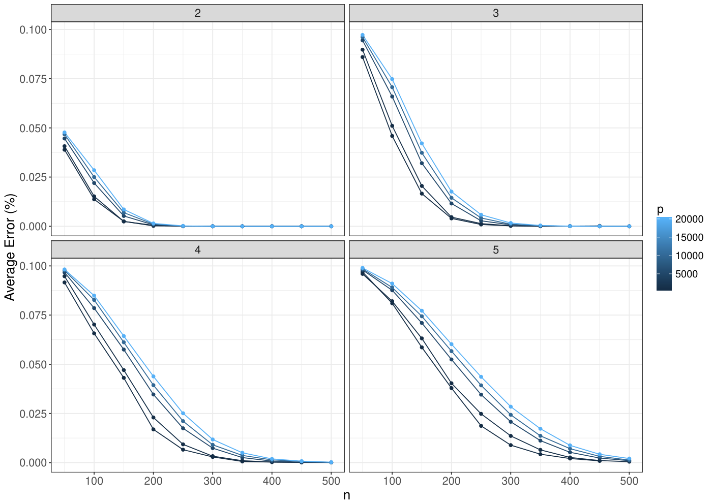
We consider sample sizes $n=50$ to $n=500$ in increments of $50$, $p=500$, $1000$, $5000$, $10000$, $20000$, and $K\in\{2,3,4,5\}$, with the samples being equally distributed among the $K$ classes in each simulation. Note, we only run the simulation for when $p>n$, as we are purely interested in results in high dimensional space. Further, we consider a sparse feature space, such that only $10\%$ of the features are discriminative, with $s_{k}$ the set of such features determined to be discriminative.

In each simulation setting, data is generated as follows: For $j\in s_{k}$, sample from the space of non-null partitions of ${\bf S}$, e.g., from a total of $M-1=15$ non-null hypotheses for $K=4$. Simulate ${\bf x}_{jmg}\sim\mathcal{N}(\mu_{jmg},1)$ where $g$ represents the group index of the normal distribution for the partition $m$ for feature $j$, and such that the mean shift for each differing normal distribution is $2$. If $j\notin s_{k}$, ${\bf x}_{i}\sim\mathcal{N}(0,1)$.

We simulate data using the above 20 times and the average total proportion incorrectly selected features (given by $E/M$) over these 20 replications is displayed in Figure 3. It is clear that as $n\rightarrow\infty$, the error rates asymptotically converge to 0, regardless of the values of $p$ and $K$. However, in the case when $p\gg n$ and $n$ small, the error increases (as to be expected) but is no bigger than $10\%$ when $K=5,p=20000$, and $n=50$.

In this study we assess the predictive performance of the multiDA algorithm with simulated data. Four simulations were considered, with two simulating under the assumption of independent features, and the other two simulating more realistic data with multivariate normal data generated using sparse covariance matrices. In all simulations, we consider predicting the four classes, with our data matrices of dimension $n=100,p=20000$. As in Section 6.3, we consider a highly sparse set of discriminative features, utilising the sets $s_{k}$ as defined previously. Finally, as before, samples are spread equally among the four classes. The specifics of simulation settings are detailed below.

Simulations with Independent Features

1. 1.

   Mean shift with independent features, equal group variances
   For $j\in s_{k}$, sample from the space of non-null partitions of ${\bf S}$ (total of 15 non null for $K=4$). Simulate ${\bf x}_{jmg}\sim\mathcal{N}(\mu_{jmg},1)$ where $g$ represents the group index of the normal distribution for the partition $m$ for feature $j$, such that the mean shift for each differing normal distribution is $0.5$. If $j\notin s_{k}$, ${\bf x}_{i}\sim\mathcal{N}(0,1)$.

2. 2.

   Mean shift with independent features, unequal group variances
   Same as 1), however, the group variances are allowed to change within each partition, such that for $j\in s_{k}$, simulate ${\bf x}_{jg}\sim\mathcal{N}(\mu_{jmg},\sigma^{2}_{jmg})$, where $\mu_{jg}$ is defined as in 1), and such that the scale in variance for each normal distribution is $1$.

Simulations with Dependent Features

For the simulations below, define the set $s_{k}$ such that $s_{1}=[1,500],s_{2}=[501,1000],s_{3}=[1001,1500]$, and $s_{4}=[1501,2000]$.

1. 3.

   Dependent features, equal group covariances
   For $i\in{\bf y}_{k},j\in s_{k}$, ${\bf x}\sim\mathcal{N}(0.5,{\boldsymbol{\Sigma}})$ and ${\bf x}_{i}\sim\mathcal{N}(0,{\boldsymbol{\Sigma}})$ for $j\notin s_{k}$. ${\boldsymbol{\Sigma}}$ is generated as a sparse covariance matrix, such that blocks of size $2000\times 2000$ have high correlation.

2. 4.

   Dependent features, unequal group covariances
   Identical to (3), except that for $i\in{\bf y}_{k},j\in s_{k}$, ${\bf x}\sim\mathcal{N}(0.5,{\boldsymbol{\Sigma}}_{k})$, as in this case we consider the scenario in which group covariances differ.

The ${\boldsymbol{\Sigma}}$ and ${\boldsymbol{\Sigma}}_{k}$ covariance matrices are constructed as follows. Let ${\bf B}_{\ell}$ be a $b\times b$ matrix where the diagonal entries and $\Delta$ percent of the off diagonal entries are generated using independent normally distributed random variables. Then the matrices ${\boldsymbol{\Sigma}}$ and ${\boldsymbol{\Sigma}}_{k}$ are constructed by taking 10 matrices ${\bf B}_{1},\ldots,{\bf B}_{10}$ with $b=2000$ with $\Delta=0.25$, forming the block diagonal matrix consisting of the blocks ${\bf B}_{1}^{T}{\bf B}_{1},\ldots,{\bf B}_{10}^{T}{\bf B}_{10}$ and then permuting the rows and columns of the resulting matrix.

50 x 5 fold cross validation results are shown in Figure 4.

We run our multiDA algorithm, among others, on three separate publicly available data sets, for benchmark data comparison. For all three datasets, we run a 50 x 5 fold cross validation, as well as report the algorithmic run times for running the algorithm once on the full data set.

TCGA Breast Cancer data

Microarray data from the Cancer Genome Atlas (TCGA) was used to classify 5 different subtypes of breast cancer, namely “Basal”, “HER2”, “Luminal A”, and “Luminal B”, as well as distinguish between healthy tissue, with the data consisting of 266 samples and a feature set of size 15803. As the breast cancer subtypes were defined intrinsically based on PAM50 gene expression levels, these genes were removed first in order to see if other complementary genes could be used in order to predict cancer subtype. Cross validation results are shown in Figure 5. Results for the multiDA algorithms were achieved using default settings for our algorithm.

Small Round Blue Cell Tumors (SRBCT) data

The SRBCT dataset (Khan et al., 2001) looks at classifying 4 classes of different childhood tumours sharing similar visual features during routine histology. These classes include Ewing’s family of tumours (EWS), neuroblastoma (NB), Burkitt’s lymphoma (BL), and rhabdomyosarcoma (RMS). Data was collected from 83 cDNA microarrays, with 1586 features present after filtering for genes with zero median absolute deviation. Cross validation results are shown in Figure 6. Results for the multiDA algorithms were achieved using default settings for our algorithm.

Melanoma data

The melanoma dataset has been analysed by (Mann et al., 2013) as a binary classification problem. The dataset consist of $n=98$ samples of Affymetrix arrays with $p=23901$ genes measured on each array. The response variable is the patient’s prognosis, which is compromised of three classes - good, middle, and poor prognosis groups. Class labels have been defined as follows, using the status of the patient and their survival times:

Samples that do not meet the criteria above are excluded, leaving $n=54$ samples for analysis. Further, we implemented a filtering step that excludes under-expressed genes (all three class medians below 7), resulting in $p=12404$ genes to be used for analysis. Cross validation results are shown in Figure 7.

Results for the multiDA algorithms were achieved using default settings except for the penalty - in which the BIC setting was used. The use of a weaker penalty is justified through an extreme trade-off between PSR and FDR. Investigation into features selected using the EBIC penalty revealed that those deemed significant by multiQDA to be driven by extreme outliers - due to the strong penalty ensuring that only those with a maximal LRT are deemed discriminative, greatly reducing the PSR. As such, we have selected the BIC penalty, acknowledging the likely increase in FDR, however improving predictive performance by increasing PSR (strong predictive performance of DQDA indicates importance of PSR).

While we recognise that run time of each algorithm depends on various factors involving hardware and implementation chosen, we provide the timings in Table 2 below as indicative in the context of the details outlined in Section 6. These times suggest that multiLDA and multiQDA both run in a reasonable amount of time in comparison to the competing methods considered in this paper.

Through simulation studies and applications on publicly available data, we are able to analyse the strengths of our multiDA classifier. Our simulation study examining the feature selection component of multiDA demonstrates the ability of multiDA to accurately select the correct feature set as the sample size increases, confirming our theoretical considerations. As the number of classes increases, the sample size needed to select the correct features increase, however this is to be expected.

Examining predictive strength through both simulations and benchmark data analysis, it is clear that the multiLDA algorithm excels when group variances are assumed to be equal (Simulations 1 and 3), and performs poorly when this assumption is not met (Simulations 2 and 4, Melanoma microarray analysis). The converse is true for multiQDA, which also shows improvements to all LDA based methods in the unequal variances cases as well as out performing plain DQDA in Simulation 2 and also showing strengths in the Melanoma example. In the independent features case for our simulation studies, the other DA methods (penLDA, NSC, DLDA, DQDA) do well as expected, however their performance is much worse in Simulation 2 (as expected). SVM has poor performance overall in both simulated and benchmark data examples, with KNN, LASSO, and RandomForest (RF) performing better in some simulations as compared to others.

It is also clear that the multiDA classifier can perform well when assumptions of independence of features is not met. This is demonstrated in Simulations 3 and 4 when we consider data with a non diagonalised covariance structure, and also in the benchmark data analysis examples, where in gene expression data we expect some degree of correlation between the features.

In all examples shown with the exception of Simulation 1, the multiDA classifiers have performed as well or better than all DA-like methods, consistently outperformed methods such as KNN and SVM, and have produced competitive results with Random Forest and the LASSO on multiple datasets.

References

- Akaike (1974) Akaike, H., 1974. A New Look at the Statistical Model Identification. IEEE Transactions on Automatic Control 19 (6), 716–723.
- Benjamini and Hochberg (1995) Benjamini, Y., Hochberg, Y., 1995. Controlling the false discovery rate: A practical and powerful approach to multiple testing. Journal of the Royal Statistical Society. Series B (Methodological) 57 (1), 289–300.
- Bickel and Levina (2004) Bickel, P. J., Levina, E., 2004. Some theory for Fisher’s linear discriminant function, ‘näive Bayes’, and some alternatives when there are many more variables than observations. Bernoulli 10 (6), 989–1010.
- Bonferroni (1936) Bonferroni, C. E., 1936. Teoria statistica delle classi e calcolo delle probabilità. Pubblicazioni del R Istituto Superiore di Scienze Economiche e Commerciali di Firenze 8, 3–62.
- Breiman (2001) Breiman, L., Oct 2001. Random forests. Machine Learning 45 (1), 5–32.
- Chen and Chen (2008) Chen, J., Chen, Z., 2008. Extended Bayesian information criteria for model selection with large model spaces. Biometrika 95 (3), 759–771.
- Clemmensen et al. (2011) Clemmensen, L., Hastie, T., Witten, D., Ersbøll, B., 2011. Sparse discriminant analysis. Technometrics 53 (4), 406–413.
- Cortes and Vapnik (1995) Cortes, C., Vapnik, V., Sep 1995. Support-vector networks. Machine Learning 20 (3), 273–297.
- Cover and Hart (1967) Cover, T., Hart, P., January 1967. Nearest neighbor pattern classification. IEEE Transactions on Information Theory 13 (1), 21–27.
- Dudoit et al. (2002) Dudoit, S., Fridlyand, J., Speed, T. P., 2002. Comparison of discrimination methods for the classification of tumors using gene expression data. Journal of the American Statistical Association 97 (457), 77–87.
- Fisher (1936) Fisher, R. A., 1936. The use of multiple measurements in taxonomic problems. Annals of Eugenics 7 (2), 179–188.
- Friedman et al. (2010) Friedman, J., Hastie, T., Tibshirani, R., 2010. Regularization paths for generalized linear models via coordinate descent. Journal of Statistical Software 33 (1), 1–22.
- Friedman (1989) Friedman, J. H., 1989. Regularized discriminant analysis. Journal of the American Statistical Association 84 (405), 165–175.
- Gasull et al. (2015) Gasull, A., López-Salcedo, J. A., Utzet, F., 2015. Maxima of Gamma random variables and other Weibull-like distributions and the Lambert W function. TEST 24 (4), 714–733.
- Hankin (2006) Hankin, R. K. S., May 2006. Additive integer partitions in R. Journal of Statistical Software, Code Snippets 16.
- Hastie et al. (2014) Hastie, T., Tibshirani, R., Narasimhan, B., Chu, G., 2014. pamr: PAM: prediction analysis for microarrays. R package version 1.55.
- Holm (1979) Holm, S., 1979. A simple sequentially rejective multiple test procedure. Scandinavian Journal of Statistics 6 (2), 65–70.
- Khan et al. (2001) Khan, J., Wei, J. S., Ringnér, M., Saal, L. H., Ladanyi, M., Westermann, F., Berthold, F., Schwab, M., Antonescu, C. R., Peterson, C., Meltzer, P. S., Jun 2001. Classification and diagnostic prediction of cancers using gene expression profiling and artificial neural networks. Nature Medicine 7, 673 –679.
- Leng (2008) Leng, C., 2008. Sparse optimal scoring for multiclass cancer diagnosis and biomarker detection using microarray data. Computational Biology and Chemistry 32 (6), 417 –425.
- Liaw and Wiener (2002) Liaw, A., Wiener, M., 2002. Classification and Regression by randomForest. R News 2 (3), 18–22.
- Lundberg et al. (2017)
Lundberg, S. M., Nair, B., Vavilala, M. S., Horibe, M., Eisses, M. J., Adams,
T., Liston, D. E., Low, D. K.-W., Newman, S.-F., Kim, J., Lee, S.-I., 2017.
Explainable machine learning predictions to help anesthesiologists prevent
hypoxemia during surgery. bioRxiv.
URL https://www.biorxiv.org/content/early/2017/10/21/206540 - Mann et al. (2013) Mann, G., Pupo, G., Campain, A., Carter, C., Schramm, S., Pianova, S., Gerega, S., De Silva, C., Lai, K., Wilmott, J., Synnott, M., Hersey, P., Kefford, R., Thompson, J., Yang, J., Scolyer, R., Feb 2013. BRAF mutation, NRAS mutation, and the absence of an immune-related expressed gene profile predict poor outcome in patients with stage III melanoma. Journal of Investigative Dermatology 133 (2), 509–517.
- Meyer et al. (2017) Meyer, D., Dimitriadou, E., Hornik, K., Weingessel, A., Leisch, F., 2017. e1071: Misc Functions of the Department of Statistics, Probability Theory Group (Formerly: E1071), TU Wien. R package version 1.6-8.
- Ormerod et al. (2017)
Ormerod, J. T., Stewart, M., Yu, W., Romanes, S. E., 2017. Bayesian hypothesis
tests with diffuse priors: Can we have our cake and eat it too?
URL arxiv.org/pdf/1710.09146.pdf - Pang et al. (2009) Pang, H., Tong, T., Zhao, H., 2009. Shrinkage-based diagonal discriminant analysis and its applications in high-dimensional data. Biometrics 65 (4), 1021–1029.
- R Core Team (2014) R Core Team, 2014. R: A Language and Environment for Statistical Computing. R Foundation for Statistical Computing, Vienna, Austria.
- Ramey (2017) Ramey, J. A., 2017. sparsediscrim: Sparse and Regularized Discriminant Analysis. R package version 0.2.4.
- Ročková and George (2014) Ročková, V., George, E. I., 2014. EMVS: The EM approach to Bayesian variable selection. Journal of the American Statistical Association 109 (506), 828–846.
- Schwarz (1978) Schwarz, G., 03 1978. Estimating the dimension of a model. The Annals of Statistics 6 (2), 461–464.
- Shao (2003) Shao, J., 2003. Mathematical Statistics. Springer Texts in Statistics. Springer.
- The Cancer Genome Atlas Network (2012) The Cancer Genome Atlas Network, Sep 2012. Comprehensive molecular portraits of human breast tumours. Nature 490, 61–70.
- Tibshirani (1996) Tibshirani, R., 1996. Regression shrinkage and selection via the lasso. Journal of the Royal Statistical Society. Series B (Methodological) 58 (1), 267–288.
- Tibshirani et al. (2003) Tibshirani, R., Hastie, T., Narasimhan, B., Chu, G., 02 2003. Class prediction by nearest shrunken centroids, with applications to dna microarrays. Statistical Science 18 (1), 104–117.
- van der Vaart (1998) van der Vaart, A. W., 1998. Asymptotic statistics, volume 3 of Cambridge Series in Statistical and Probabilistic Mathematics. Cambridge University Press, Cambridge.
- Venables and Ripley (2002) Venables, W. N., Ripley, B. D., 2002. Modern Applied Statistics with S, 4th Edition. Springer, New York.
- Vuong (1989) Vuong, Q. H., 1989. Likelihood ratio tests for model selection and nonnested hypotheses. Econometrica 57 (2), 307–333.
- Wickham (2009) Wickham, H., 2009. ggplot2: Elegant Graphics for Data Analysis. Springer-Verlag New York.
- Witten (2015) Witten, D., 2015. penalizedLDA: Penalized classification using Fisher’s Linear Discriminant. R package version 1.1.
- Witten and Tibshirani (2011) Witten, D. M., Tibshirani, R., 2011. Penalized classification using Fisher’s linear discriminant. Journal of the Royal Statistical Society: Series B (Statistical Methodology) 73 (5), 753–772.
Appendix A - Theory
Let for some true parameter vector . Define the log-likelihood for variable and hypothesis as with corresponding MLE and “pseudo-true” value of as
respectively. We will assume conditions on the likelihood and parameter space such that for , . Using the theory summarised in Ormerod et al. (2017) based on Vuong (1989) and van der Vaart (1998) we have two main cases to consider.
- •
[Underfitting case] – Suppose for some . Then
and so .
[Overfitting case] – Suppose for some and let . Then
The following lemma will be useful later.
Lemma 1 (Gasull et al., 2015): If , , are independent random variables, and , then
as where is a Gumbel distributed random variable.
Define and . Here is the set of true variables over the th set of hypotheses, and is the union of over-fitting and true models over the th set of hypotheses. We define and decompose the the error as
where , and .
Note that for the index is summation does not include since the null model cannot be an overfitting model. Next, we consider where the true model is used as the null hypothesis and rewrite as
where . Using a chi-square approximation over the set of over-fitting models in place of LRT statistics with we obtain an approximation of given by
where , the last line follows from Lemma 1 with being independent Gumbel distributions. Note that provided . Similarly, for we have
where , the above may be positive or negative, and . The only potentially problematic term occurs for when since . For this case provided
Which is true provided . Hence, .