Connecting Weighted Automata and Recurrent Neural Networks through Spectral Learning
Guillaume Rabusseau11footnotemark: 1 22footnotemark: 2 Tianyu Li11footnotemark: 1 33footnotemark: 3 Doina Precup11footnotemark: 1 33footnotemark: 3 grabus@iro.umontreal.ca tianyu.li@mail.mcgill.ca dprecup@cs.mcgill.ca
Abstract
In this paper, we unravel a fundamental connection between weighted finite automata (WFAs) and second-order recurrent neural networks (2-RNNs): in the case of sequences of discrete symbols, WFAs and 2-RNNs with linear activation functions are expressively equivalent. Motivated by this result, we build upon a recent extension of the spectral learning algorithm to vector-valued WFAs and propose the first provable learning algorithm for linear 2-RNNs defined over sequences of continuous input vectors. This algorithm relies on estimating low rank sub-blocks of the so-called Hankel tensor, from which the parameters of a linear 2-RNN can be provably recovered. The performances of the proposed method are assessed in a simulation study.
1 Introduction
Many tasks in natural language processing, computational biology, reinforcement learning, and time series analysis rely on learning with sequential data, i.e. estimating functions defined over sequences of observations from training data. Weighted finite automata (WFAs) and recurrent neural networks (RNNs) are two powerful and flexible classes of models which can efficiently represent such functions. On the one hand, WFAs are tractable, they encompass a wide range of machine learning models (they can for example compute any probability distribution defined by a hidden Markov model (HMM) [12] and can model the transition and observation behavior of partially observable Markov decision processes [43]) and they offer appealing theoretical guarantees. In particular, the so-called spectral methods for learning HMMs [22], WFAs [4, 5] and related models [18, 7], provide an alternative to Expectation-Maximization based algorithms that is both computationally efficient and consistent. On the other hand, RNNs are remarkably expressive models — they can represent any computable function [41] — and they have successfully tackled many practical problems in speech and audio recognition [19, 31, 15], but their theoretical analysis is difficult. Even though recent work provides interesting results on their expressive power [24, 48] as well as alternative training algorithms coming with learning guarantees [40], the theoretical understanding of RNNs is still limited.
In this work, we bridge a gap between these two classes of models by unraveling a fundamental connection between WFAs and second-order RNNs (2-RNNs): when considering input sequences of discrete symbols, 2-RNNs with linear activation functions and WFAs are one and the same, i.e. they are expressively equivalent and there exists a one-to-one mapping between the two classes (moreover, this mapping conserves model sizes). While connections between finite state machines (e.g. deterministic finite automata) and recurrent neural networks have been noticed and investigated in the past (see e.g. [16, 32]), to the best of our knowledge this is the first time that such a rigorous equivalence between linear 2-RNNs and weighted automata is explicitly formalized. More precisely, we pinpoint exactly the class of recurrent neural architectures to which weighted automata are equivalent, namely second-order RNNs with linear activation functions. This result naturally leads to the observation that linear 2-RNNs are a natural generalization of WFAs (which take sequences of discrete observations as inputs) to sequences of continuous vectors, and raises the question of whether the spectral learning algorithm for WFAs can be extended to linear 2-RNNs. The second contribution of this paper is to show that the answer is in the positive: building upon the spectral learning algorithm for vector-valued WFAs introduced recently in [37], we propose the first provable learning algorithm for second-order RNNs with linear activation functions. Our learning algorithm relies on estimating sub-blocks of the so-called Hankel tensor, from which the parameters of a 2-linear RNN can be recovered using basic linear algebra operations. One of the key technical difficulties in designing this algorithm resides in estimating these sub-blocks from training data where the inputs are sequences of continuous vectors. We leverage multilinear properties of linear 2-RNNs and the fact that the Hankel sub-blocks can be reshaped into higher-order tensors of low tensor train rank (a result we believe is of independent interest) to perform this estimation efficiently using matrix sensing and tensor recovery techniques. As a proof of concept, we validate our theoretical findings in a simulation study on toy examples where we experimentally compare different recovery methods and investigate the robustness of our algorithm to noise and rank mis-specification. We also show that refining the estimator returned by our algorithm using stochastic gradient descent can lead to significant improvements.
Summary of contributions.
We formalize a strict equivalence between weighted automata and second-order RNNs with linear activation functions (Section 3), showing that linear 2-RNNs can be seen as a natural extension of (vector-valued) weighted automata for input sequences of continuous vectors. We then propose a consistent learning algorithm for linear 2-RNNs (Section 4). The relevance of our contributions can be seen from two perspectives. First, while learning feed-forward neural networks with linear activation functions is a trivial task (it reduces to linear or reduced-rank regression), this is not at all the case for recurrent architectures with linear activation functions; to the best of our knowledge, our algorithm is the first consistent learning algorithm for the class of functions computed by linear second-order recurrent networks. Second, from the perspective of learning weighted automata, we propose a natural extension of WFAs to continuous inputs and our learning algorithm addresses the long-standing limitation of the spectral learning method to discrete inputs.
Related work.
Combining the spectral learning algorithm for WFAs with matrix completion techniques (a problem which is closely related to matrix sensing) has been theoretically investigated in [6]. An extension of probabilistic transducers to continuous inputs (along with a spectral learning algorithm) has been proposed in [39]. The connections between tensors and RNNs have been previously leveraged to study the expressive power of RNNs in [24] and to achieve model compression in [48, 47, 44]. Exploring relationships between RNNs and automata has recently received a renewed interest [34, 9, 29]. In particular, such connections have been explored for interpretability purposes [45, 3] and the ability of RNNs to learn classes of formal languages has been investigated in [2]. Connections between the tensor train decomposition and WFAs have been previously noticed in [10, 11, 36]. The predictive state RNN model introduced in [13] is closely related to 2-RNNs and the authors propose to use the spectral learning algorithm for predictive state representations to initialize a gradient based algorithm; their approach however comes without theoretical guarantees. Lastly, a provable algorithm for RNNs relying on the tensor method of moments has been proposed in [40] but it is limited to first-order RNNs with quadratic activation functions (which do not encompass linear 2-RNNs).
The proofs of the results given in the paper can be found in the supplementary material.
2 Preliminaries
In this section, we first present basic notions of tensor algebra before introducing second-order recurrent neural network, weighted finite automata and the spectral learning algorithm. We start by introducing some notation. For any integer we use to denote the set of integers from to . We use to denote the smallest integer greater or equal to . For any set , we denote by the set of all finite-length sequences of elements of (in particular, will denote the set of strings on a finite alphabet ). We use lower case bold letters for vectors (e.g. ), upper case bold letters for matrices (e.g. ) and bold calligraphic letters for higher order tensors (e.g. ). We use to denote the th canonical basis vector of (where the dimension will always appear clearly from context). The identity matrix will be written as . The th row (resp. column) of a matrix will be denoted by (resp. ). This notation is extended to slices of a tensor in the straightforward way. If and , we use to denote the Kronecker product between vectors, and its straightforward extension to matrices and tensors. Given a matrix , we use to denote the column vector obtained by concatenating the columns of . The inverse of is denoted by , its Moore-Penrose pseudo-inverse by , and the transpose of its inverse by ; the Frobenius norm is denoted by and the nuclear norm by .
Tensors.
We first recall basic definitions of tensor algebra; more details can be found in [27]. A tensor can simply be seen as a multidimensional array . The mode- fibers of are the vectors obtained by fixing all indices except the th one, e.g. . The th mode matricization of is the matrix having the mode- fibers of for columns and is denoted by . The vectorization of a tensor is defined by . In the following always denotes a tensor of size .
The mode- matrix product of the tensor and a matrix is a tensor denoted by . It is of size and is defined by the relation . The mode- vector product of the tensor and a vector is a tensor defined by . It is easy to check that the -mode product satisfies where we assume compatible dimensions of the tensor and the matrices and .
Given strictly positive integers satisfying , we use the notation to denote the th order tensor obtained by reshaping into a tensor11 1 Note that the specific ordering used to perform matricization, vectorization and such a reshaping is not relevant as long as it is consistent across all operations. of size . In particular we have and .
A rank tensor train (TT) decomposition [33] of a tensor consists in factorizing into the product of core tensors , and is defined22 2 The classical definition of the TT-decomposition allows the rank to be different for each mode, but this definition is sufficient for the purpose of this paper. by
for all indices ; we will use the notation to denote such a decomposition. A tensor network representation of this decomposition is shown in Figure 1. While the problem of finding the best approximation of TT-rank of a given tensor is NP-hard [20], a quasi-optimal SVD based compression algorithm (TT-SVD) has been proposed in [33]. It is worth mentioning that the TT decomposition is invariant under change of basis: for any invertible matrix and any core tensors , we have .
Second-order RNNs.
A second-order recurrent neural network (2-RNN) [17, 35, 28]33 3 Second-order reccurrent architectures have also been successfully used more recently, see e.g. [42] and [46]. with hidden units can be defined as a tuple where is the initial state, is the transition tensor, and is the output matrix, with and being the input and output dimensions respectively. A 2-RNN maps any sequence of inputs to a sequence of outputs defined for any by
| (1) |
where and are activation functions. Alternatively, one can think of a 2-RNN as computing a function mapping each input sequence to the corresponding final output . While and are usually non-linear component-wise functions, we consider in this paper the case where both and are the identity, and we refer to the resulting model as a linear 2-RNN. For a linear 2-RNN , the function is multilinear in the sense that, for any integer , its restriction to the domain is multilinear. Another useful observation is that linear 2-RNNs are invariant under change of basis: for any invertible matrix , the linear 2-RNN is such that . A linear 2-RNN with states is called minimal if its number of hidden units is minimal (i.e. any linear 2-RNN computing has at least hidden units).
Weighted automata and spectral learning.
Vector-valued weighted finite automaton (vv-WFA) have been introduced in [37] as a natural generalization of weighted automata from scalar-valued functions to vector-valued ones. A -dimensional vv-WFA with states is a tuple where is the initial weights vector, is the matrix of final weights, and is the transition matrix for each symbol in a finite alphabet . A vv-WFA computes a function defined by
for each word . We call a vv-WFA minimal if its number of states is minimal. Given a function we denote by the number of states of a minimal vv-WFA computing (which is set to if cannot be computed by a vv-WFA).
The spectral learning algorithm for vv-WFAs relies on the following fundamental theorem relating the rank of a function to its Hankel tensor , which is defined by for all .
Theorem 1 ([37]).
Let and let be its Hankel tensor. Then .
The vv-WFA learning algorithm leverages the fact that the proof of this theorem is constructive: one can recover a vv-WFA computing from any low rank factorization of . In practice, a finite sub-block of the Hankel tensor is used to recover the vv-WFA, where are finite sets of prefixes and suffixes forming a complete basis for , i.e. such that . More details can be found in [37].
3 A Fundamental Relation between WFAs and Linear 2-RNNs
We start by unraveling a fundamental connection between vv-WFAs and linear 2-RNNs: vv-WFAs and linear 2-RNNs are expressively equivalent for representing functions defined over sequences of discrete symbols. Moreover, both models have the same capacity in the sense that there is a direct correspondence between the hidden units of a linear 2-RNN and the states of a vv-WFA computing the same function. More formally, we have the following theorem.
Theorem 2.
Any function that can be computed by a vv-WFA with states can be computed by a linear 2-RNN with hidden units. Conversely, any function that can be computed by a linear 2-RNN with hidden units on sequences of one-hot vectors (i.e. canonical basis vectors) can be computed by a WFA with states.
More precisely, the WFA with states and the linear 2-RNN with hidden units, where is defined by for all , are such that for all sequences of input symbols , where for each the input vector is the one-hot encoding of the symbol .
This result first implies that linear 2-RNNs defined over sequence of discrete symbols (using one-hot encoding) can be provably learned using the spectral learning algorithm for WFAs/vv-WFAs; indeed, these algorithms have been proved to return consistent estimators. Let us stress again that, contrary to the case of feed-forward architectures, learning recurrent networks with linear activation functions is not a trivial task. Furthermore, Theorem 2 reveals that linear 2-RNNs are a natural generalization of classical weighted automata to functions defined over sequences of continuous vectors (instead of discrete symbols). This spontaneously raises the question of whether the spectral learning algorithms for WFAs and vv-WFAs can be extended to the general setting of linear 2-RNNs; we show that the answer is in the positive in the next section.
4 Spectral Learning of Linear 2-RNNs
In this section, we extend the learning algorithm for vv-WFAs to linear 2-RNNs, thus at the same time addressing the limitation of the spectral learning algorithm to discrete inputs and providing the first consistent learning algorithm for linear second-order RNNs.
4.1 Recovering 2-RNNs from Hankel Tensors
We first present an identifiability result showing how one can recover a linear 2-RNN computing a function from observable tensors extracted from some Hankel tensor associated with . Intuitively, we obtain this result by reducing the problem to the one of learning a vv-WFA. This is done by considering the restriction of to canonical basis vectors; loosely speaking, since the domain of this restricted function is isomorphic to , this allows us to fall back onto the setting of sequences of discrete symbols.
Given a function , we define its Hankel tensor by
for all , which is infinite in two of its modes. It is easy to see that is also the Hankel tensor associated with the function mapping any sequence to . Moreover, in the special case where can be computed by a linear 2-RNN, one can use the multilinearity of to show that , giving us some intuition on how one could learn by learning a vv-WFA computing using the spectral learning algorithm. That is, given a large enough sub-block of for some prefix and suffix sets , one should be able to recover a vv-WFA computing and consequently a linear 2-RNN computing using Theorem 2. Before devoting the remaining of this section to formalize this intuition (leading to Theorem 3), it is worth observing that while this approach is sound, it is not realistic since it requires observing entries of the Hankel tensor , which implies having access to input/output examples where the inputs are sequences of canonical basis vectors; This issue will be discussed in more details and addressed in the next section.
For the sake of clarity, we present the learning algorithm for the particular case where there exists an such that the prefix and suffix sets consisting of all sequences of length , that is , forms a complete basis for (i.e. the sub-block of the Hankel tensor is such that ). This assumption allows us to present all the key elements of the algorithm in a simpler way, the technical details needed to lift this assumption are given in the supplementary material.
For any integer , we define the finite tensor of order by
Observe that for any integer , the tensor can be obtained by reshaping a finite sub-block of the Hankel tensor . When is computed by a linear -RNN, we have the useful property that, for any integer ,
| (2) |
for any sequence of inputs (which can be shown using the multilinearity of ). Another fundamental property of the tensors is that they are of low tensor train rank. Indeed, for any , one can check that (the tensor network representation of this decomposition is shown in Figure 2). This property will be particularly relevant to the learning algorithm we design in the following section, but it is also a fundamental relation that deserves some attention on its own: it implies in particular that, beyond the classical relation between the rank of the Hankel matrix and the number states of a minimal WFA computing , the Hankel matrix possesses a deeper structure intrinsically connecting weighted automata to the tensor train decomposition. We now state the main result of this section, showing that a (minimal) linear 2-RNN computing a function can be exactly recovered from sub-blocks of the Hankel tensor .
Theorem 3.
Let be a function computed by a minimal linear -RNN with hidden units and let be an integer such that .
Then, for any and such that , the linear 2-RNN defined by
is a minimal linear -RNN computing .
First observe that such an integer exists under the assumption that forms a complete basis for . It is also worth mentioning that a necessary condition for is that , i.e. must be of the order .
4.2 Hankel Tensors Recovery from Linear Measurements
We showed in the previous section that, given the Hankel tensors , and , one can recover a linear 2-RNN computing if it exists. This first implies that the class of functions that can be computed by linear 2-RNNs is learnable in Angluin’s exact learning model [1] where one has access to an oracle that can answer membership queries (e.g. what is the value computed by the target on ?) and equivalence queries (e.g. is my current hypothesis equal to the target ?). While this fundamental result is of significant theoretical interest, assuming access to such an oracle is unrealistic. In this section, we show that a stronger learnability result can be obtained in a more realistic setting, where we only assume access to randomly generated input/output examples where .
The key observation is that such an input/output example can be seen as a linear measurement of the Hankel tensor . Indeed, we have
where . Hence, by regrouping output examples into the matrix and the corresponding input vectors into the matrix , one can recover by solving the linear system , which has a unique solution whenever is of full column rank. This naturally leads to the following theorem, whose proof relies on the fact that will be of full column rank whenever and the components of each for are drawn independently from a continuous distribution over (w.r.t. the Lebesgue measure).
Theorem 4.
Let be a minimal linear 2-RNN with hidden units computing a function , and let be an integer44 4 Note that the theorem can be adapted if such an integer does not exists (see supplementary material). such that . Suppose we have access to datasets for where the entries of each are drawn independently from the standard normal distribution and where each .
Then, if for , the linear 2-RNN returned by Algorithm 1 with the least-squares method satisfies with probability one.
A few remarks on this theorem are in order. The first observation is that the datasets , and can either be drawn independently or not (e.g. the sequences in can be prefixes of the sequences in but it is not necessary). In particular, the result still holds when the datasets are constructed from a unique dataset of input/output sequences with , where for any . Observe that having access to such input/output training sequences is not an unrealistic assumption: for example when training RNNs for language modeling the output is the conditional probability vector of the next symbol, and for classification tasks the output is the one-hot encoded label for all time steps. Lastly, when the outputs are noisy, one can solve the least-squares problem to approximate the Hankel tensors; we will empirically evaluate this approach in Section 5 and we defer its theoretical analysis in the noisy setting to future work.
4.3 Leveraging the low rank structure of the Hankel tensors
While the least-squares method is sufficient to obtain the theoretical guarantees of Theorem 4, it does not leverage the low rank structure of the Hankel tensors , and . We now propose three alternative recovery methods to leverage this structure, whose sample efficiency will be assessed in a simulation study in Section 5 (deriving improved sample complexity guarantees using these methods is left for future work). In the noiseless setting, we first propose to replace solving the linear system with a nuclear norm minimization problem (see line 6 of Algorithm 1), thus leveraging the fact that is potentially of low matrix rank. We also propose to use iterative hard thresholding (IHT) [23] and its tensor counterpart TIHT [38], which are based on the classical projected gradient descent algorithm and have shown to be robust to noise in practice. These two methods are implemented in lines 9-12 of Algorithm 1. There, the project method either projects onto the manifold of low rank matrices using SVD (IHT) or projects onto the manifold of tensors with TT-rank (TIHT).
The low rank structure of the Hankel tensors can also be leveraged to improve the scalability of the learning algorithm. One can check that the computational complexity of Algorithm 1 is exponential in the maximum sequence length: indeed, building the matrix in line 2 is already in , where is in turn equal to and . Focusing on the TIHT recovery method, a careful analysis shows that the computational complexity of the algorithm is in
where and is the number of iterations of the loop on line 9. Thus, in its present form, our approach cannot scale to high dimensional inputs and long sequences. However, one can leverage the low tensor train rank structure of the Hankel tensors to circumvent this issue: by storing both the estimates of the Hankel tensors and the matrices in TT format (with decompositions of ranks and respectively), all the operations needed to implement Algorithm 1 with the TIHT recovery method can be performed in time (more details can be found in the supplementary material). By leveraging the tensor train structure, one can thus lift the dependency on by paying the price of an increased cubic complexity in the number of examples and the number of states . While the dependency on the number of states is not a major issue ( should be negligible w.r.t. ), the dependency on can quickly become prohibitive for realistic application scenario. Fortunately, this issue can be dealt with by using mini-batches of training data for the gradient updates on line 10 instead of the whole dataset , in which case the overall complexity of Algorithm 1 becomes where is the mini-batch size (the overall algorithm in TT format is summarized in Algorithm 2 in the supplementary material).
5 Experiments
In this section, we perform experiments55 5 https://github.com/litianyu1993/learning_2RNN on two toy examples to compare how the choice of the recovery method (LeastSquares, NuclearNorm, IHT and TIHT) affects the sample efficiency of Algorithm 1. Additional experiments on real data can be found in Appendix D. We also include comparisons with RNNs with long short term memory (LSTM) units [21] and report the performances obtained by refining the solution returned by our algorithm (with the TIHT recovery method) using stochastic gradient descent (TIHT+SGD).
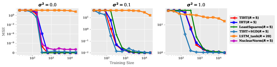
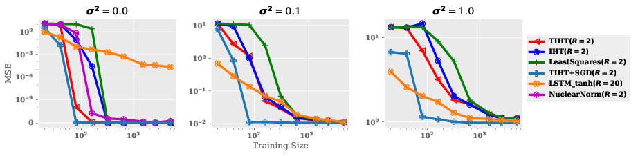
We perform two experiments. In the first one, we randomly generate a linear 2-RNN with units computing a function by drawing the entries of all parameters independently from the normal distribution . The training data consists of independently drawn sets for with , where each and where the outputs can be noisy, i.e. where for some noise variance . In the second experiment, the goal is to learn a simple arithmetic function computing the sum of the running differences between the two components of a sequence of -dimensional vectors, i.e. where . The training datasets are generated using the same process as above and a constant entry equal to one is added to all the input vectors to encode a bias term (one can check that the resulting function can be computed by a linear 2-RNN with hidden units).
We run the experiments for different sizes of training data ranging from to (we set ) and we compare the different methods in terms of mean squared error (MSE) on a test set of sequences of length generated in the same way as the training data (note that the training data only contains sequences of length up to ).
We report the performances of (non-linear) RNNs with a single layer of LSTM with hidden units (with activation functions66 6 We also tried training LSTMs with linear recurrent activation functions on the two tasks but they always performed worse than non-linear ones.) and one fully-connected output layer, trained using the Adam optimizer [25] with learning rate 0.001. We also use Adam with learning rate 0.001 to refine the models returned by TIHT with stochastic gradient descent SGD (we tried directly training a linear 2-RNN from random initializations using SGD as well but this approach always failed to return a good model). The IHT/TIHT methods sometimes returned aberrant models (due to numerical instabilities), we used the following scheme to circumvent this issue: when the training MSE of the hypothesis was greater than the one of the zero function, the zero function was returned instead (we applied this scheme to all other methods in the experiments).
The results are reported in Figure 3 and 4 where we see that all recovery methods of Algorithm 1 lead to consistent estimates of the target function given enough training data. This is the case even in the presence of noise (in which case more samples are needed to achieve the same accuracy, as expected). We can also see that IHT and TIHT are overall more sample efficient than the other methods (especially with noisy data), showing that taking the low rank structure of the Hankel tensors into account is profitable. Moreover, TIHT tends to perform better than its matrix counterpart, confirming our intuition that leveraging the tensor train structure is beneficial. While LSTMs obtain good performances on the addition task, they struggle to recover the random linear 2-RNN in the first task (despite our efforts at hyper-parameter tuning and architecture search). In the meantime, refining the TIHT models using SGD almost always leads to significant improvements (especially under the noisy setting), matching or outperforming the performances of RNNs on the two tasks. Lastly, we show the effect of rank mis-specification in Figure 5: as one can expect, when the rank parameter is over-estimated Algorithm 1 still converges to the target function but it requires more samples (when the rank parameter was underestimated all algorithms did not learn at all).

6 Conclusion and Future Directions
We proposed the first provable learning algorithm for second-order RNNs with linear activation functions: we showed that linear 2-RNNs are a natural extension of vv-WFAs to the setting of input sequences of continuous vectors (rather than discrete symbol) and we extended the vv-WFA spectral learning algorithm to this setting. We believe that the results presented in this paper open a number of exciting and promising research directions on both the theoretical and practical perspectives. We first plan to use the spectral learning estimate as a starting point for gradient based methods to train non-linear 2-RNNs. More precisely, linear 2-RNNs can be thought of as 2-RNNs using LeakyRelu activation functions with negative slope , therefore one could use a linear 2-RNN as initialization before gradually reducing the negative slope parameter during training. The extension of the spectral method to linear 2-RNNs also opens the door to scaling up the classical spectral algorithm to problems with large discrete alphabets (which is a known caveat of the spectral algorithm for WFAs) since it allows one to use low dimensional embeddings of large vocabularies (using e.g. word2vec or latent semantic analysis). From the theoretical perspective, we plan on deriving learning guarantees for linear 2-RNNs in the noisy setting (e.g. using the PAC learnability framework). Even though it is intuitive that such guarantees should hold (given the continuity of all operations used in our algorithm), we believe that such an analysis may entail results of independent interest. In particular, analogously to the matrix case studied in [8], obtaining rate optimal convergence rates for the recovery of the low TT-rank Hankel tensors from rank one measurements is an interesting direction; such a result could for example allow one to improve the generalization bounds provided in [6] for spectral learning of general WFAs.
Acknowledgements
This work was done while G. Rabusseau was an IVADO postdoctoral scholar at McGill University.
References
- [1] Dana Angluin. Queries and concept learning. Machine learning, 2(4):319–342, 1988.
- [2] Enes Avcu, Chihiro Shibata, and Jeffrey Heinz. Subregular complexity and deep learning. CLASP Papers in Computational Linguistics, page 20, 2017.
- [3] Stéphane Ayache, Rémi Eyraud, and Noé Goudian. Explaining black boxes on sequential data using weighted automata. In Proceedings of ICGI, pages 81–103, 2018.
- [4] Raphaël Bailly, François Denis, and Liva Ralaivola. Grammatical inference as a principal component analysis problem. In Proceedings of ICML, pages 33–40, 2009.
- [5] Borja Balle, Xavier Carreras, Franco M Luque, and Ariadna Quattoni. Spectral learning of weighted automata. Machine learning, 96(1-2):33–63, 2014.
- [6] Borja Balle and Mehryar Mohri. Spectral learning of general weighted automata via constrained matrix completion. In Proceedings of NIPS, pages 2159–2167, 2012.
- [7] Byron Boots, Sajid M. Siddiqi, and Geoffrey J. Gordon. Closing the learning-planning loop with predictive state representations. International Journal of Robotics Research, 30(7):954–966, 2011.
- [8] T Tony Cai, Anru Zhang, et al. Rop: Matrix recovery via rank-one projections. The Annals of Statistics, 43(1):102–138, 2015.
- [9] Yining Chen, Sorcha Gilroy, Andreas Maletti, Jonathan May, and Kevin Knight. Recurrent neural networks as weighted language recognizers. In Proceedings of NAACL-HLT, pages 2261–2271, 2018.
- [10] Andrew Critch. Algebraic geometry of hidden Markov and related models. PhD thesis, University of California, Berkeley, 2013.
- [11] Andrew Critch and Jason Morton. Algebraic geometry of matrix product states. SIGMA, 10(095):095, 2014.
- [12] François Denis and Yann Esposito. On rational stochastic languages. Fundamenta Informaticae, 86(1, 2):41–77, 2008.
- [13] Carlton Downey, Ahmed Hefny, Byron Boots, Geoffrey J Gordon, and Boyue Li. Predictive state recurrent neural networks. In Proceedings of NIPS, pages 6055–6066, 2017.
- [14] Herbert Federer. Geometric measure theory. Springer, 2014.
- [15] Felix A Gers, Jürgen Schmidhuber, and Fred Cummins. Learning to forget: Continual prediction with LSTM. Neural Computation, 12(10):2451–2471, 2000.
- [16] C Lee Giles, Clifford B Miller, Dong Chen, Hsing-Hen Chen, Guo-Zheng Sun, and Yee-Chun Lee. Learning and extracting finite state automata with second-order recurrent neural networks. Neural Computation, 4(3):393–405, 1992.
- [17] C Lee Giles, Guo-Zheng Sun, Hsing-Hen Chen, Yee-Chun Lee, and Dong Chen. Higher order recurrent networks and grammatical inference. In Proceedings of NIPS, pages 380–387, 1990.
- [18] Hadrien Glaude and Olivier Pietquin. PAC learning of probabilistic automaton based on the method of moments. In Proceedings of ICML, pages 820–829, 2016.
- [19] Alex Graves, Abdel-rahman Mohamed, and Geoffrey Hinton. Speech recognition with deep recurrent neural networks. In Proceedings of ICASSP, pages 6645–6649. IEEE, 2013.
- [20] Christopher J Hillar and Lek-Heng Lim. Most tensor problems are np-hard. Journal of the ACM (JACM), 60(6):45, 2013.
- [21] Sepp Hochreiter and Jürgen Schmidhuber. Long short-term memory. Neural computation, 9(8):1735–1780, 1997.
- [22] Daniel J. Hsu, Sham M. Kakade, and Tong Zhang. A spectral algorithm for learning hidden markov models. In Proceedings of COLT, 2009.
- [23] Prateek Jain, Raghu Meka, and Inderjit S Dhillon. Guaranteed rank minimization via singular value projection. In Proceedings of NIPS, pages 937–945, 2010.
- [24] Valentin Khrulkov, Alexander Novikov, and Ivan Oseledets. Expressive power of recurrent neural networks. In Proceedings of ICLR, 2018.
- [25] Diederik P Kingma and Jimmy Ba. Adam: A method for stochastic optimization. arXiv preprint arXiv:1412.6980, 2014.
- [26] Stefan Klus, Patrick Gelß, Sebastian Peitz, and Christof Schütte. Tensor-based dynamic mode decomposition. Nonlinearity, 31(7):3359, 2018.
- [27] Tamara G Kolda and Brett W Bader. Tensor decompositions and applications. SIAM review, 51(3):455–500, 2009.
- [28] YC Lee, Gary Doolen, HH Chen, GZ Sun, Tom Maxwell, HY Lee, and C Lee Giles. Machine learning using a higher order correlation network. Physica D: Nonlinear Phenomena, 22(1-3):276–306, 1986.
- [29] Tianyu Li, Guillaume Rabusseau, and Doina Precup. Nonlinear weighted finite automata. In Proceedings of AISTATS, pages 679–688, 2018.
- [30] Qin Lin, Christian Hammerschmidt, Gaetano Pellegrino, and Sicco Verwer. Short-term time series forecasting with regression automata. 2016.
- [31] Tomáš Mikolov, Stefan Kombrink, Lukáš Burget, Jan Černockỳ, and Sanjeev Khudanpur. Extensions of recurrent neural network language model. In Proceedings of ICASSP, pages 5528–5531. IEEE, 2011.
- [32] Christian W Omlin and C Lee Giles. Constructing deterministic finite-state automata in recurrent neural networks. Journal of the ACM (JACM), 43(6):937–972, 1996.
- [33] Ivan V Oseledets. Tensor-train decomposition. SIAM Journal on Scientific Computing, 33(5):2295–2317, 2011.
- [34] Hao Peng, Roy Schwartz, Sam Thomson, and Noah A Smith. Rational recurrences. In Proceedings of EMNLP, pages 1203–1214, 2018.
- [35] Jordan B Pollack. The induction of dynamical recognizers. In Connectionist Approaches to Language Learning, pages 123–148. Springer, 1991.
- [36] Guillaume Rabusseau. A Tensor Perspective on Weighted Automata, Low-Rank Regression and Algebraic Mixtures. PhD thesis, Aix-Marseille Université, 2016.
- [37] Guillaume Rabusseau, Borja Balle, and Joelle Pineau. Multitask spectral learning of weighted automata. In Proceedings of NIPS, pages 2585–2594, 2017.
- [38] Holger Rauhut, Reinhold Schneider, and Željka Stojanac. Low rank tensor recovery via iterative hard thresholding. Linear Algebra and its Applications, 523:220–262, 2017.
- [39] Adria Recasens and Ariadna Quattoni. Spectral learning of sequence taggers over continuous sequences. In Proceedings of ECML, pages 289–304, 2013.
- [40] Hanie Sedghi and Anima Anandkumar. Training input-output recurrent neural networks through spectral methods. arXiv preprint arXiv:1603.00954, 2016.
- [41] Hava T Siegelmann and Eduardo D Sontag. On the computational power of neural nets. In Proceedings of COLT, pages 440–449. ACM, 1992.
- [42] Ilya Sutskever, James Martens, and Geoffrey E Hinton. Generating text with recurrent neural networks. In Proceedings of ICML, pages 1017–1024, 2011.
- [43] Michael Thon and Herbert Jaeger. Links between multiplicity automata, observable operator models and predictive state representations: a unified learning framework. Journal of Machine Learning Research, 16:103–147, 2015.
- [44] Andros Tjandra, Sakriani Sakti, and Satoshi Nakamura. Compressing recurrent neural network with tensor train. In Proceedings of IJCNN, pages 4451–4458. IEEE, 2017.
- [45] Gail Weiss, Yoav Goldberg, and Eran Yahav. Extracting automata from recurrent neural networks using queries and counterexamples. In Proceedings of ICML, pages 5244–5253, 2018.
- [46] Yuhuai Wu, Saizheng Zhang, Ying Zhang, Yoshua Bengio, and Ruslan R Salakhutdinov. On multiplicative integration with recurrent neural networks. In Proceedings of NIPS, pages 2856–2864, 2016.
- [47] Yinchong Yang, Denis Krompass, and Volker Tresp. Tensor-train recurrent neural networks for video classification. In Proceedings of ICML, pages 3891–3900, 2017.
- [48] Rose Yu, Stephan Zheng, Anima Anandkumar, and Yisong Yue. Long-term forecasting using tensor-train rnns. arXiv preprint arXiv:1711.00073, 2017.
Connecting Weighted Automata and Recurrent Neural Networks through Spectral Learning
(Supplementary Material)
Appendix A Proofs
A.1 Proof of Theorem 2
Theorem.
Any function that can be computed by a vv-WFA with states can be computed by a linear 2-RNN with hidden units. Conversely, any function that can be computed by a linear 2-RNN with hidden units on sequences of one-hot vectors (i.e. canonical basis vectors) can be computed by a WFA with states.
More precisely, the WFA with states and the linear 2-RNN with hidden units, where is defined by for all , are such that for all sequences of input symbols , where for each the input vector is the one-hot encoding of the symbol .
Proof.
We first show by induction on that, for any sequence , the hidden state computed by (see Eq. (1)) on the corresponding one-hot encoded sequence satisfies . The case is immediate. Suppose the result true for sequences of length up to . One can check easily check that for any index . Using the induction hypothesis it then follows that
To conclude, we thus have
A.2 Proof of Theorem 3
Theorem.
Let be a function computed by a minimal linear -RNN with hidden units and let be an integer such that .
Then, for any and such that , the linear 2-RNN defined by
is a minimal linear -RNN computing .
Proof.
Let and be such that Define the tensors
of order and respectively, and let and . Using the identity for any , one can easily check the following identities:
Let . We will show that , and , which will entail the results since linear 2-RNN are invariant under change of basis (see Section 2). First observe that . Indeed, we have where we used the fact that (resp. ) is of full column rank (resp. row rank) for the last equality.
The following derivations then follow from basic tensor algebra:
which concludes the proof. ∎
A.3 Proof of Theorem 4
Theorem.
Let be a minimal linear 2-RNN with hidden units computing a function , and let be an integer77 7 Note that the theorem can be adapted if such an integer does not exists (see supplementary material). such that .
Suppose we have access to datasets for where the entries of each are drawn independently from the standard normal distribution and where each .
Then, whenever for each , the linear 2-RNN returned by Algorithm 1 with the least-squares method satisfies with probability one.
Proof.
We just need to show for each that, under the hypothesis of the Theorem, the Hankel tensors computed in line 4 of Algorithm 1 are equal to the true Hankel tensors with probability one. Recall that these tensors are computed by solving the least-squares problem
where is the matrix with rows for each . Since and since the solution of the least-squares problem is unique as soon as is of full column rank, we just need to show that this is the case with probability one when the entries of the vectors are drawn at random from a standard normal distribution. The result will then directly follow by applying Theorem 3.
We will show that the set
has Lebesgue measure in as soon as , which will imply that it has probability under any continuous probability, hence the result. For any , we denote by the matrix with rows . One can easily check that if and only if is of rank strictly less than , which is equivalent to the determinant of being equal to . Since this determinant is a polynomial in the entries of the vectors , is an algebraic subvariety of . It is then easy to check that the polynomial is not uniformly 0 when . Indeed, it suffices to choose the vectors such that the family spans the whole space (which is possible since we can choose arbitrarily any of the elements of this family), hence the result. In conclusion, is a proper algebraic subvariety of and hence has Lebesgue measure zero [14, Section 2.6.5].
∎
Appendix B Lifting the simplifying assumption
We now show how all our results still hold when there does not exist an such that . Recall that this simplifying assumption followed from assuming that the sets form a complete basis for the function defined by . We first show that there always exists an integer such that forms a complete basis for . Let be a linear 2-RNN with hidden units computing (i.e. such that ). It follows from Theorem 2 and from the discussion at the beginning of Section 4.1 that there exists a vv-WFA computing and it is easy to check that . This implies by Theorem 1. Since converges to as grows to infinity, there exists an such that the finite sub-block of satisfies , i.e. such that forms a complete basis for .
Now consider the finite sub-blocks and of defined by
for any and any . One can check that Theorem 3 holds by replacing mutatis mutandi by , by , by and by .
To conclude, it suffices to observe that both and can be constructed from the entries for the tensors for , which can be recovered (or estimated in the noisy setting) using the techniques described in Section 4.2 (corresponding to lines 2-12 of Algorithm 1).
We thus showed that linear 2-RNNs can be provably learned even when there does not exist an such that . In this setting, one needs to estimate enough of the tensors to reconstruct a complete sub-block of the Hankel tensor (along with the corresponding tensor and matrix ) and recover the linear 2-RNN by applying Theorem 3. In addition, one needs to have access to sufficiently large datasets for each rather than only the three datasets mentioned in Theorem 4. However the data requirement remains the same in the case where we assume that each of the datasets is constructed from a unique training dataset of input/output sequences.
Appendix C Leveraging the tensor train structure for computational efficiency
The overall learning algorithm using the TIHT recovery method in TT format is summarized in Algorithm 2. The key ingredients to improve the complexity of Algorithm 1 are (i) to estimate the gradient using mini-batches of data and (ii) to directly use the TT format to represent and perform operations on the tensors and the tensors defined by
| (3) |
where is the size of a mini-batch of training data ( is of TT-rank by design and it can easily be shown that is of TT-rank at most , cf. Eq. (4)). Then, all the operations of the algorithm can be expressed in terms of these tensors and performed efficiently in TT format. More precisely, the products and sums needed to compute the gradient update on line 6 can be performed in . After the gradient update, the tensor has TT-rank at most but can be efficiently projected back to a tensor of TT-rank using the tensor train rounding operation [33] in (which is the operation dominating the complexity of the whole algorithm). The subsequent operations on line 10 can be performed efficiently in the TT format in (using the method described in [26] to compute the pseudo-inverses of the matrices and ). The overall complexity of Algorithm 2 is thus in where is the number of iterations of the inner loop.
| (4) |
Appendix D Real Data Experiment on Wind Speed Prediction
Besides the synthetic data experiments we showed in the paper, we have also conducted experiments on real data. The data that we use for the these experiments is from TUDelft88 8 http://weather.tudelft.nl/csv/. Specifically, we use the data from Rijnhaven station as described in [30], which proposed a regression automata model and performed various experiments on the dataset we mentioned above. The data contains wind speed and related information at the Rijnhaven station from 2013-04-22 at 14:55:00 to 2018-10-20 at 11:40:00 and was collected every five minutes. To compare to the results in [30], we strictly followed the data preprocessing procedure described in the paper. We use the data from 2013-04-23 to 2015-10-12 as training data and the rest as our testing data. The paper uses SAX as a preprocessing method to discretize the data. However, as there is no need to discretize data for our algorithm, we did not perform this procedure. For our method, we set the length and we use the general algorithm described in Appendix B. We calculate hourly averages of the wind speed, and predict one/three/six hour(s) ahead, as in [30]. For our methods we use a linear 2-RNN with 10 states. Averages over 5 runs of this experiment for one-hour-ahead, three-hour-ahead, six-hour-ahead prediction error can be found in Table 1, 2 and 3. The results for RA, RNN and persistence are taken directly from [30]. We see that while TIHT+SGD performs slightly worse than ARIMA and RA for one-hour-ahead prediction, it outperforms all other methods for three-hours and six-hours ahead predictions (and the superiority w.r.t. other methods increases as the prediction horizon gets longer).
| Method | TIHT | TIHT+SGD |
|
ARIMA | RNN | Persistence | ||
|---|---|---|---|---|---|---|---|---|
| RMSE | 0.573 | 0.519 | 0.500 | 0.496 | 0.606 | 0.508 | ||
| MAPE | 21.35 | 18.79 | 18.58 | 18.74 | 24.48 | 18.61 | ||
| MAE | 0.412 | 0.376 | 0.363 | 0.361 | 0.471 | 0.367 |
| Method | TIHT | TIHT+SGD |
|
ARIMA | RNN | Persistence | ||
|---|---|---|---|---|---|---|---|---|
| RMSE | 0.868 | 0.854 | 0.872 | 0.882 | 1.002 | 0.893 | ||
| MAPE | 33.98 | 31.70 | 32.52 | 33.165 | 37.24 | 33.29 | ||
| MAE | 0.632 | 0.624 | 0.632 | 0.642 | 0.764 | 0.649 |
| Method | TIHT | TIHT+SGD |
|
ARIMA | RNN | Persistence | ||
|---|---|---|---|---|---|---|---|---|
| RMSE | 1.234 | 1.145 | 1.205 | 1.227 | 1.261 | 1.234 | ||
| MAPE | 49.08 | 44.88 | 46.809 | 48.02 | 47.03 | 48.11 | ||
| MAE | 0.940 | 0.865 | 0.898 | 0.919 | 0.944 | 0.923 |